
Determination of Current and Future Extreme Sea Levels at the Local Scale in Port-Bouët Bay (Côte d’Ivoire)
 , , and
Abstract
:1. Introduction
2. Materials and Methods
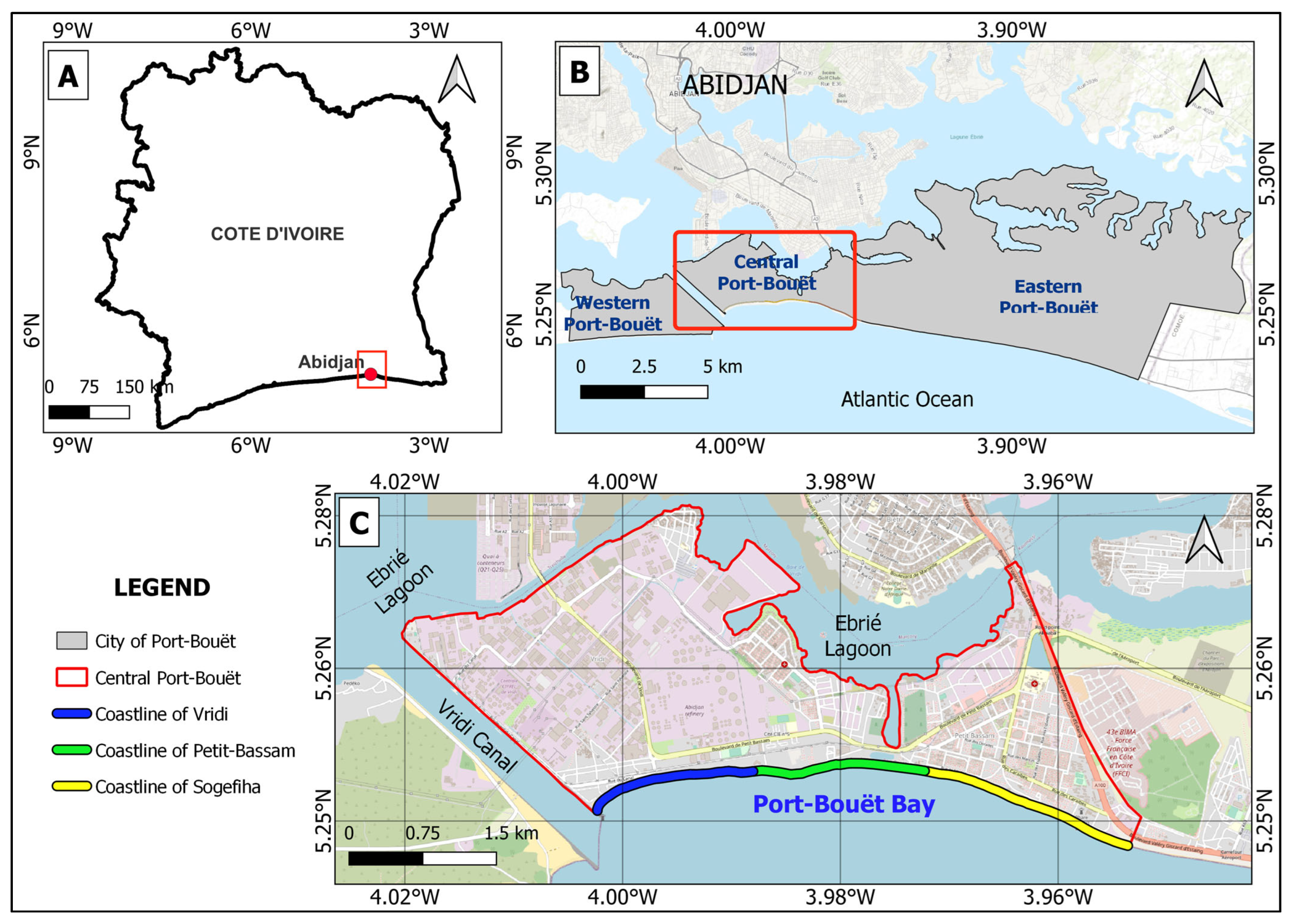
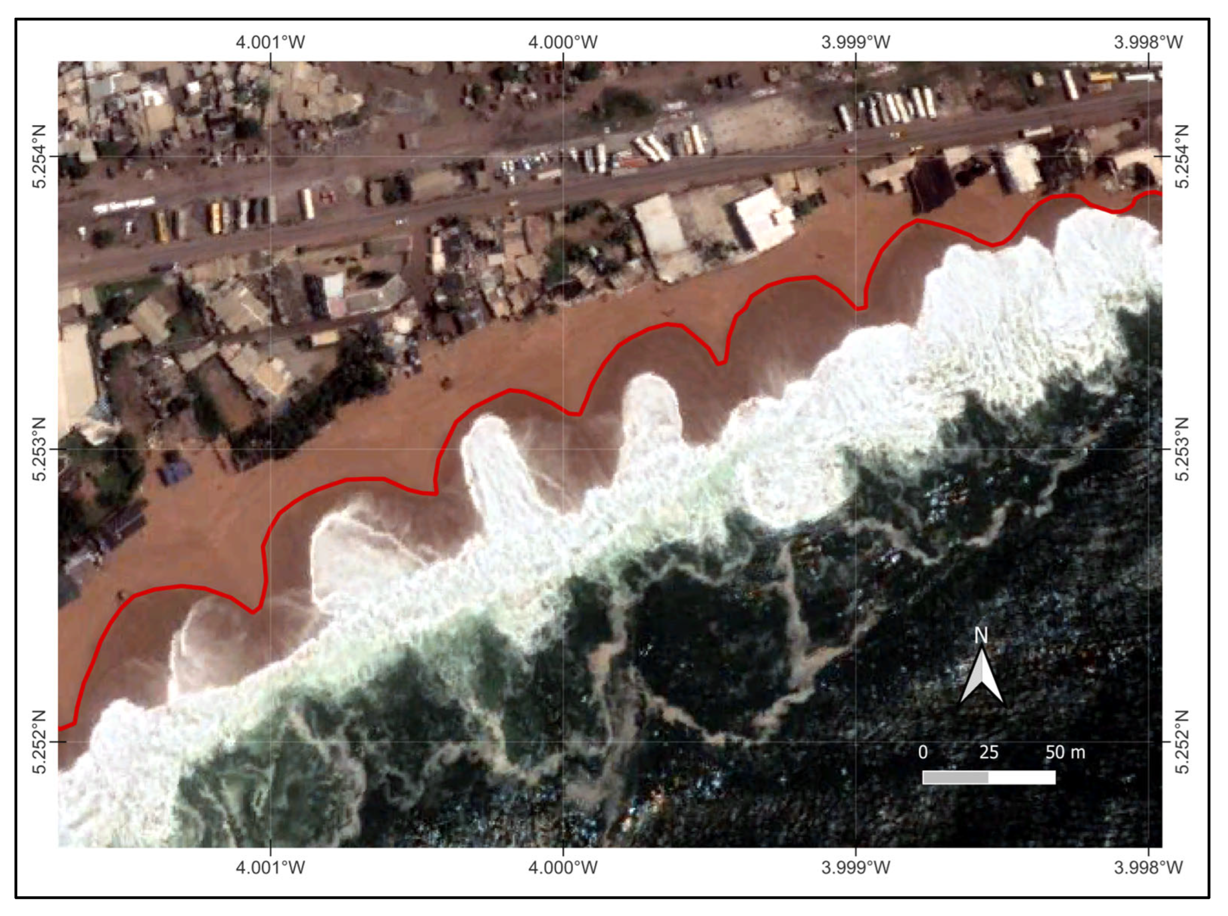
2.1. Study Area
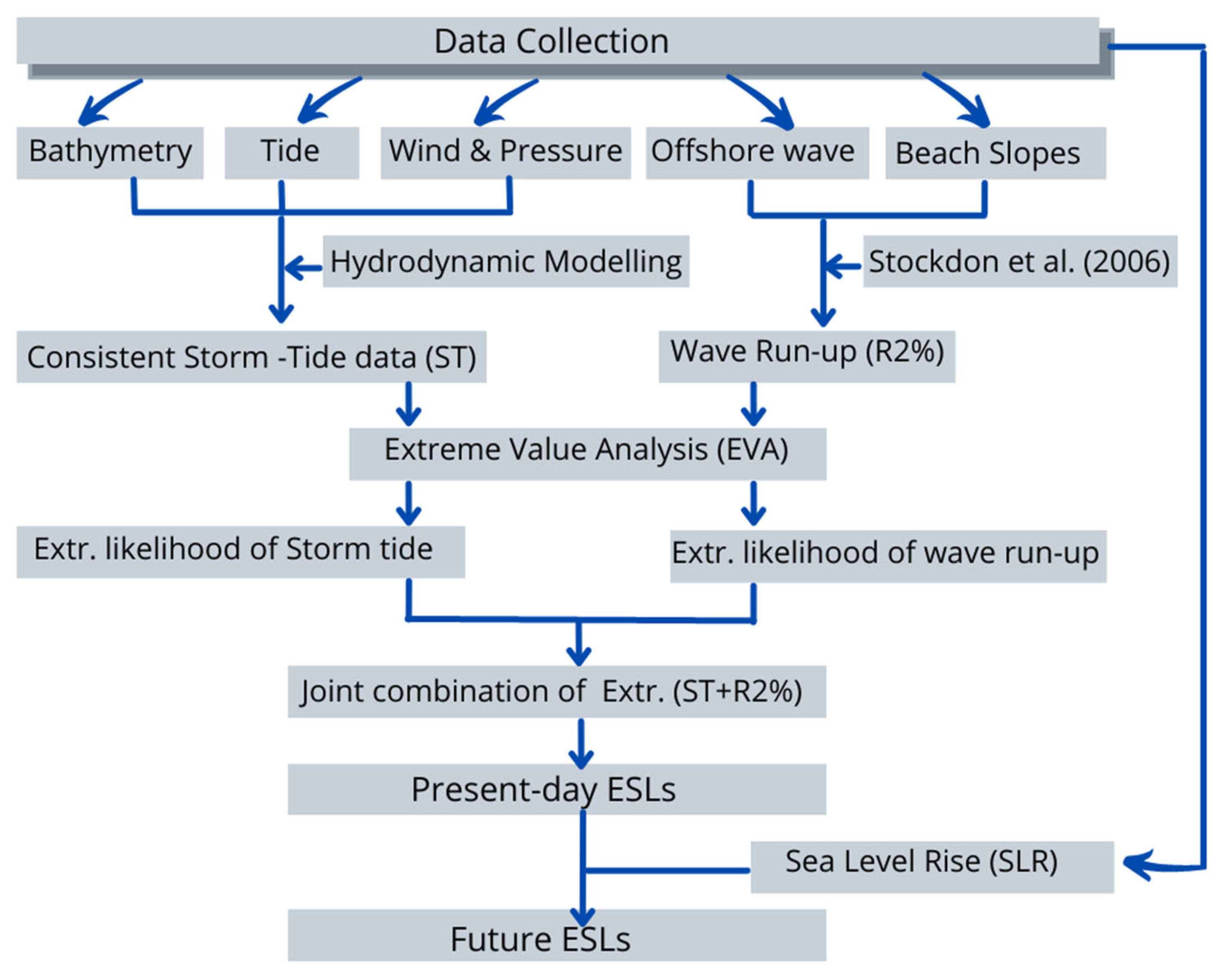
2.2. Approach Overview
2.3. Data

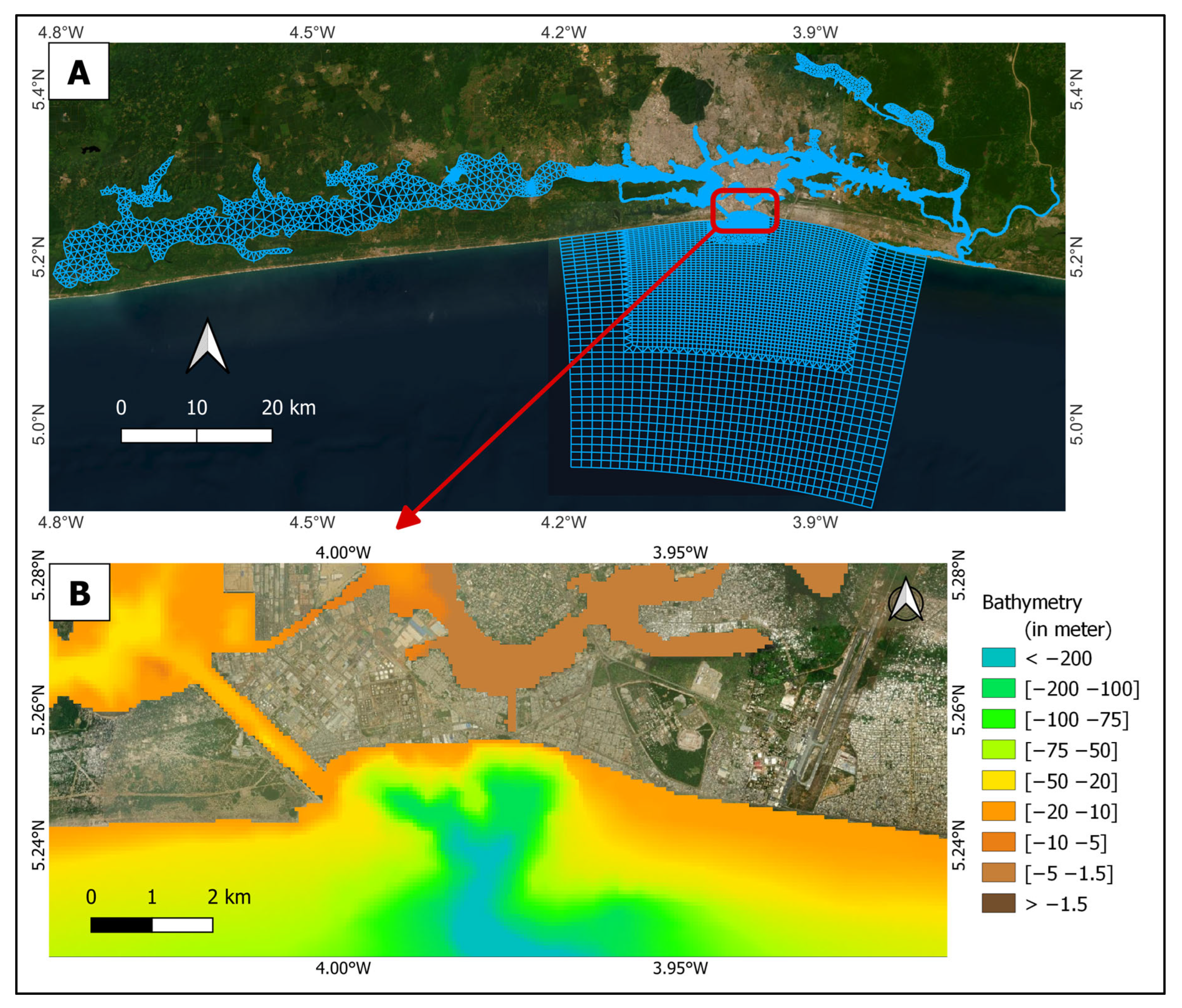
2.4. Methods
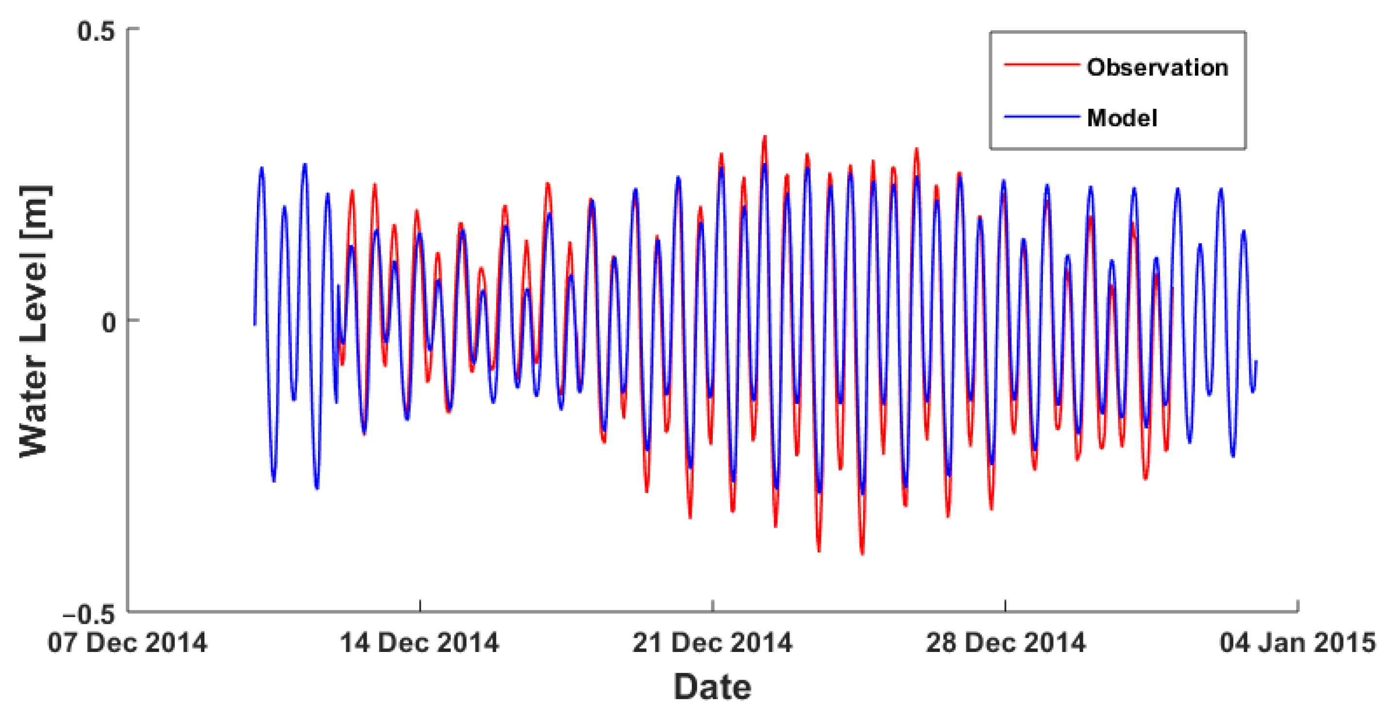
2.4.1. Storm Tide Modelling
2.4.2. Wave Run-up Calculation
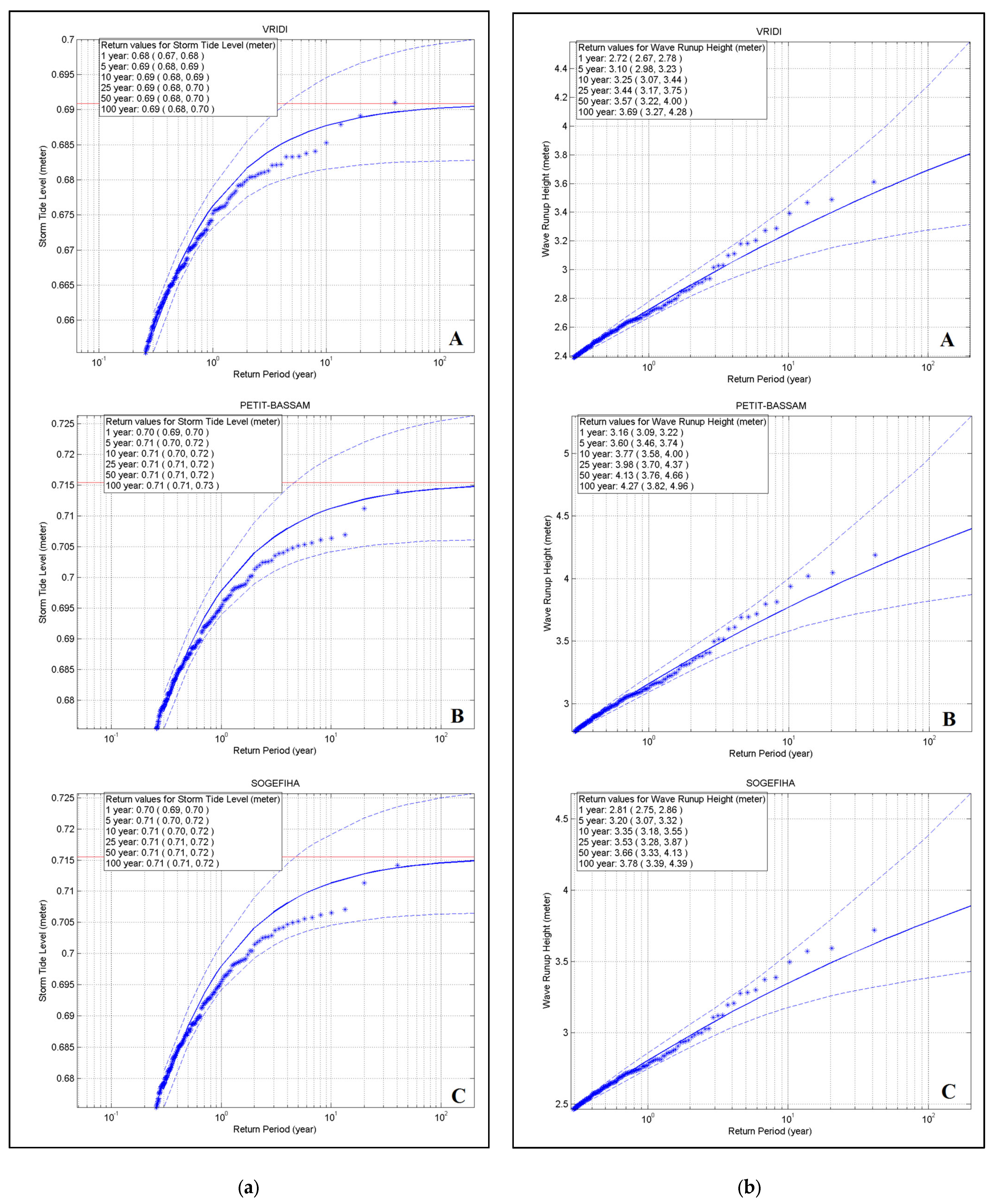
2.4.3. Extreme Value Analysis
- Defining a high threshold.
- Extracting the exceedances time-series, i.e., selection of all values above the defined threshold.
- Declustering: This step consists of selecting the peak value within each cluster in order to ensure the independency of excesses over the defined threshold and therefore justify the use of the GPD model.
- Finally, the calculation of return level: Values that are exceeded in any given year.
2.4.4. Joint Probability Analysis (JPM)
2.5. ESL Scenario Design
- For the present-day ESLs, six scenarios are defined based on the probability of occurrence of extreme events. These correspond to the best-fit return values for each of the 1, 5, 10, 25, 50- and 100-year return periods.
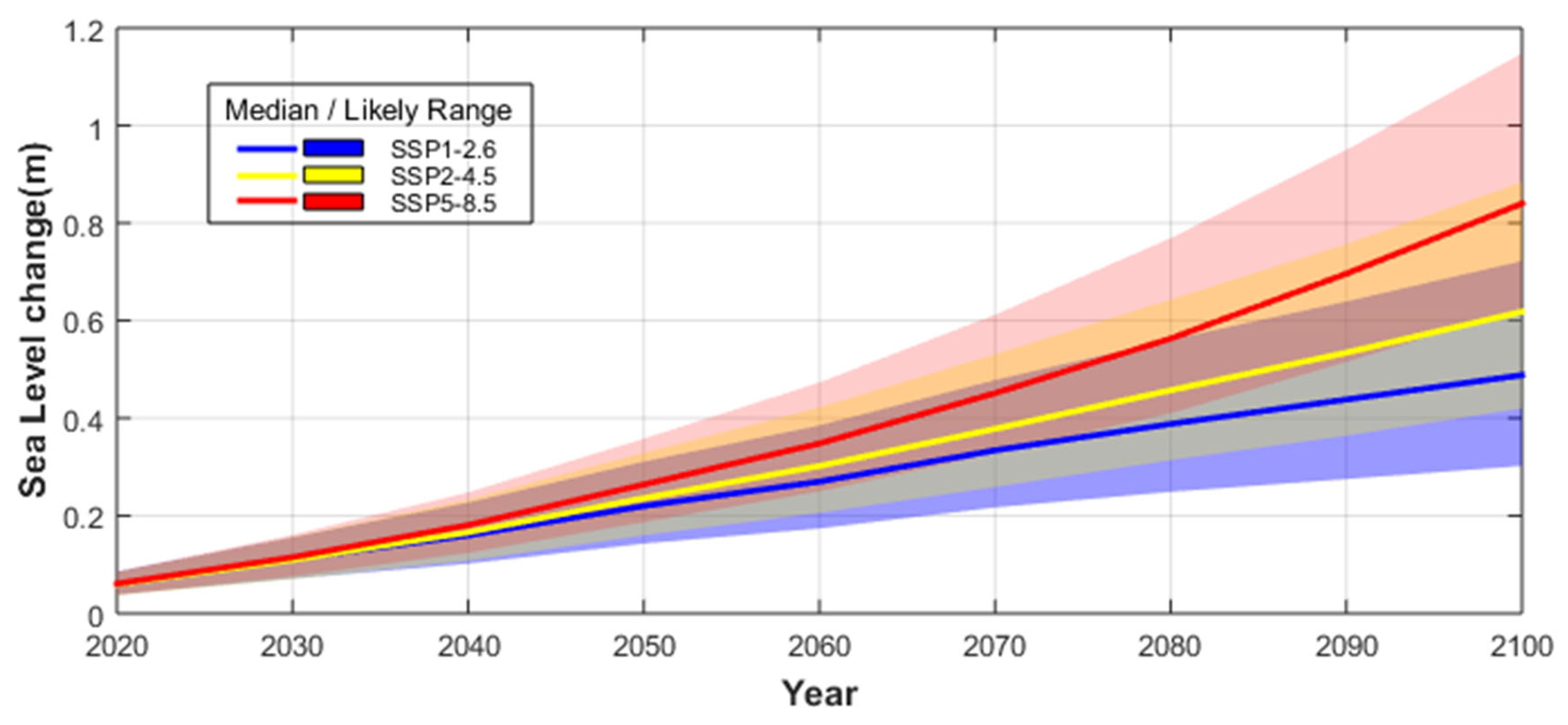
- For future ESLs, scenarios are designed by combining the present-day ESLs scenarios with the SLR scenarios. Therefore, the present-day ESL return levels are combined with three medium confidence SLR scenarios (precisely SSP1-2.6, SSP2-4.5 and SSP5-8.5) for the years 2030, 2050 and 2100. This combination follows (3) as defined in the approach overview section.
3. Results
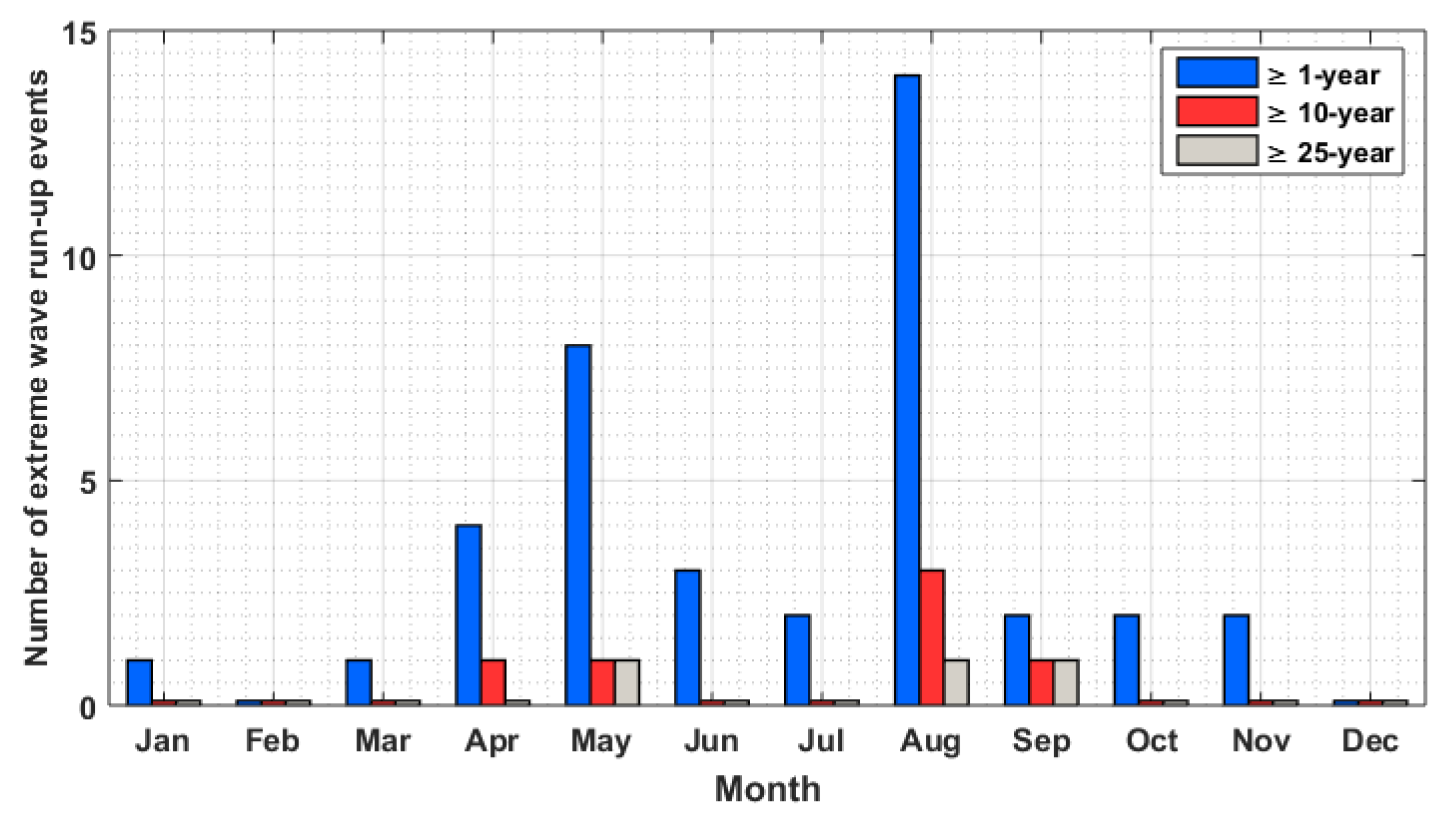
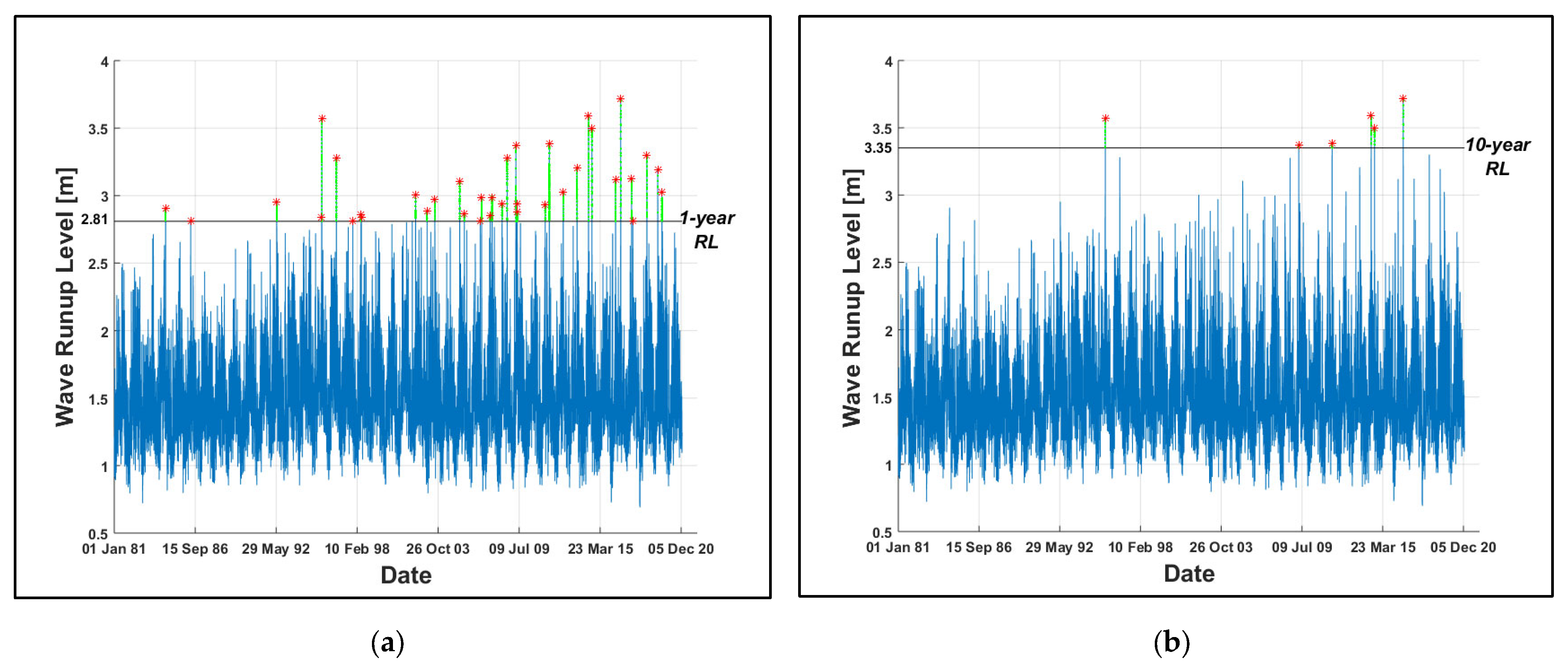
3.1. Extreme Storm Tide and Wave Run-Up
3.2. Present-Day ESLs
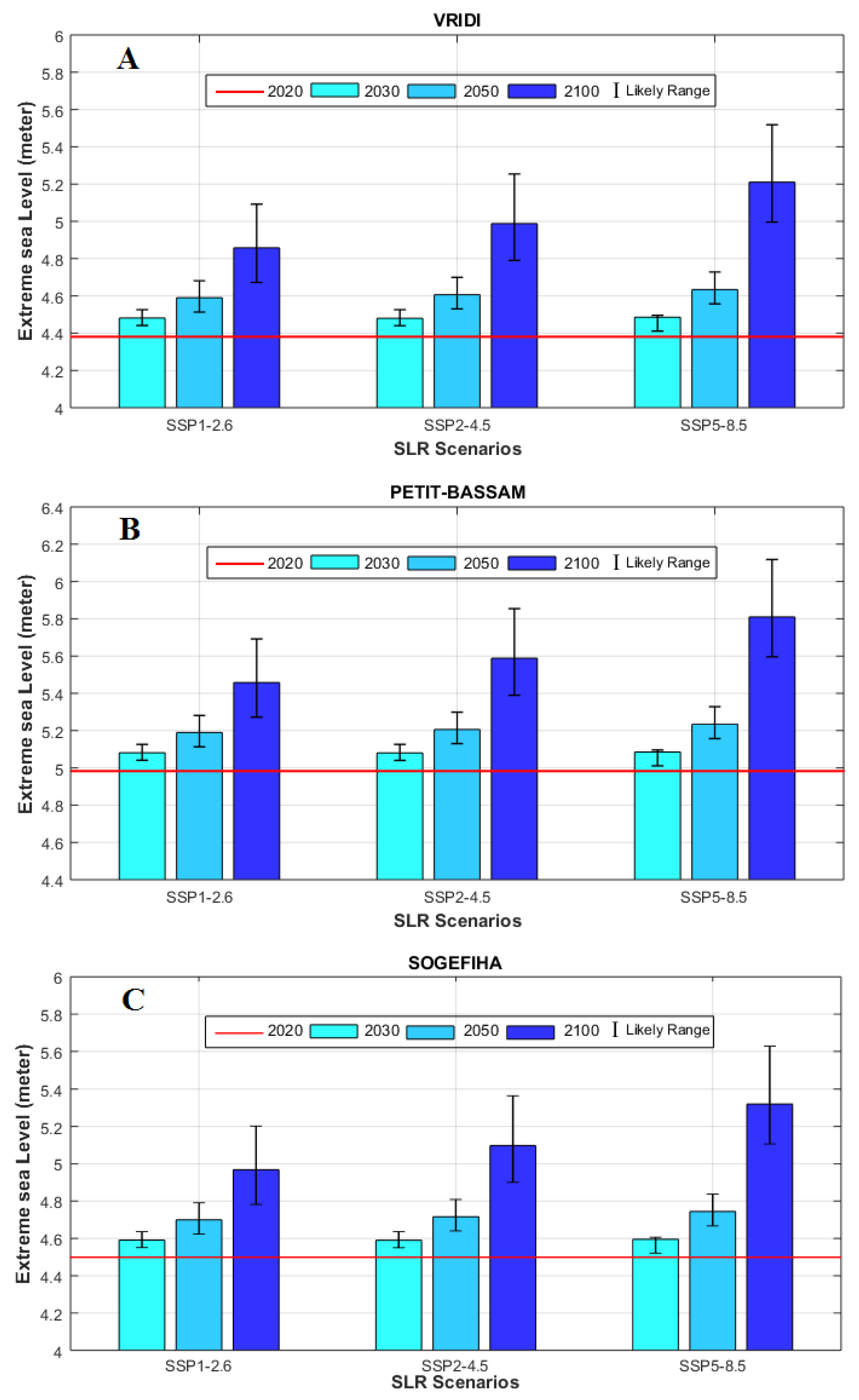
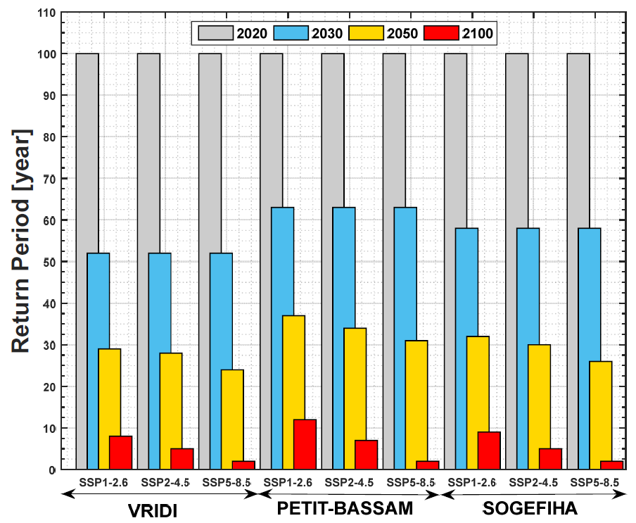
3.3. Future ESLs
4. Discussion
- Selection of dataset length
- Determination of representative beach slopes
- Independence between ESL components
5. Conclusions
Supplementary Materials
Author Contributions
Funding
Institutional Review Board Statement
Informed Consent Statement
Data Availability Statement
Acknowledgments
Conflicts of Interest
References
- Wadey, M.P.; Nicholls, R.J.; Hutton, C. Defences and Inundation Coastal Flooding in the Solent: An Integrated Analysis of Defences and Inundation. Water 2012, 4, 430–459. [Google Scholar] [CrossRef] [Green Version]
- Lang, A.; Mikolajewicz, U. The long-term variability of extreme sea levels in the German Bight. Ocean Sci. 2019, 15, 651–668. [Google Scholar] [CrossRef] [Green Version]
- Sayol, J.M.; Marcos, M. Assessing Flood Risk Under Sea Level Rise and Extreme Sea Levels Scenarios: Application to the Ebro Delta (Spain). J. Geophys. Res. Oceans 2018, 123, 794–811. [Google Scholar] [CrossRef] [Green Version]
- Carvajal, M.; Winckler, P.; Garreaud, R.; Igualt, F.; Contreras-López, M.; Averil, P.; Cisternas, M.; Gubler, A.; Breuer, W.A. Extreme sea levels at Rapa Nui (Easter Island) during intense atmospheric rivers. Nat. Hazards 2021, 106, 1619–1637. [Google Scholar] [CrossRef]
- Zhang, H.; Sheng, J. Estimation of extreme sea levels over the eastern continental shelf of North America. J. Geophys. Res. Oceans 2013, 118, 6253–6273. [Google Scholar] [CrossRef]
- Pirazzoli, P.A.; Tomasin, A.; Ullmann, A. Extreme sea levels in two northern Mediterranean areas. Méditerranée 2007, 108, 59–68. [Google Scholar] [CrossRef]
- Khan, F.A.; Ali-Khan, T.M.; Afan, H.A.; Sherif, M.; Sefelnasr, A.; El-Shafie, A. Complex extreme sea levels prediction analysis: Karachi coast case study. Entropy 2020, 22, 549. [Google Scholar] [CrossRef] [PubMed]
- Fredriksson, C.; Tajvidi, N.; Hanson, H.; Larson, M. Statistical Analysis of Extreme Sea Water Level at the Falsterbo Peninsula, South Sweden. Vatten J. Water Manag. Res. 2016, 72, 129–142. [Google Scholar]
- Cissé, C.O.T.; Almar, R.; Youm, J.P.M.; Jolicoeur, S.; Taveneau, A.; Sy, B.A.; Sakho, I.; Sow, B.A.; Dieng, H. Extreme Coastal Water Levels Evolution at Dakar (Senegal, West Africa). Climate 2022, 11, 6. [Google Scholar] [CrossRef]
- Cissé, C.O.T.; Brempong, E.K.; Taveneau, A.; Almar, R.; Sy, B.A.; Angnuureng, D.B. Extreme coastal water levels with potential flooding risk at the low-lying Saint Louis city, Senegal (West Africa). Front. Mar. Sci. 2022, 9, 993644. [Google Scholar] [CrossRef]
- Sreeraj, P.; Swapna, P.; Krishnan, R.; Nidheesh, A.G.; Sandeep, N. Extreme sea level rise along the Indian Ocean coastline: Observations and 21st century projections. Environ. Res. Lett. 2022, 17, 114016. [Google Scholar] [CrossRef]
- Menéndez, M.; Woodworth, P.L. Changes in extreme high water levels based on a quasi-global tide-gauge data set. J. Geophys. Res. Oceans 2010, 115, 1–15. [Google Scholar] [CrossRef] [Green Version]
- Walsh, K.J.E.; Mcinnes, K.L.; Mcbride, J.L. Climate change impacts on tropical cyclones and extreme sea levels in the South Pacific—A regional assessment. Glob. Planet. Change 2012, 80–81, 149–164. [Google Scholar] [CrossRef]
- Watson, P.J. Determining Extreme Still Water Levels for Design and Planning Purposes Incorporating Sea Level Rise. Atmosphere 2022, 13, 95. [Google Scholar] [CrossRef]
- Percival, S.; Teeuw, R. A methodology for urban micro-scale coastal flood vulnerability and risk assessment and mapping. Nat. Hazards 2019, 97, 1–23. [Google Scholar] [CrossRef] [Green Version]
- Oppenheimer, M.; Glavovic, B.C.; Hinkel, J.; van de Wal, R.; Magnan, A.K.; Abd-Elgawad, A.; Cai, R.; Cifuentes-Jara, M.; DeConto, R.M.; Ghosh, T.; et al. Sea level rise and implications for low-lying islands, coasts and communities. In IPCC Special Report on Ocean and Cryosphere in a Changing Climate; Pörtner, H.-O., Roberts, D.C., Masson-Delmotte, V., Zhai, P., Tignor, M., Poloczanska, E., Mintenbeck, K., Alegría, A., Nicolai, M., Okem, A., et al., Eds.; Cambridge University Press: Cambridge, UK; New York, NY, USA, 2019; pp. 321–445. [Google Scholar] [CrossRef]
- Weisse, R.; Bella, D.; Menéndez, M.; Méndez, F.; Nicholls, R.J.; Umgiesser, G.; Willems, P. Changing extreme sea levels along European coasts. Coast. Eng. 2014, 87, 4–14. [Google Scholar] [CrossRef] [Green Version]
- Vousdoukas, M.I.; Mentaschi, L.; Feyen, L.; Voukouvalas, E. Extreme sea levels on the rise along Europe’ s coasts Earth’ s Future. Earth’s Future 2017, 5, 1–20. [Google Scholar] [CrossRef]
- Wong, T.E.; Sheets, H.; Torline, T.; Zhang, M. Evidence for Increasing Frequency of Extreme Coastal Sea Levels. Front. Clim. 2022, 4, 24. [Google Scholar] [CrossRef]
- Konan, K.E.; Abe, J.; Aka, K.; Neumeier, U.; Nyessen, J.; Ozer, A. Impacts des houles exceptionnelles sur le littoral ivoirien du Golfe de Guinée. Géomorphologie Relief Process. Environ. 2016, 22, 105–120. [Google Scholar] [CrossRef]
- Tomety, S.F. Analyse des Statistiques de Vagues au Nord du Golfe de Guinée (Côte d’Ivoire, Ghana, Bénin, Nigéria) Dans le Cadre du Suivi de L’érosion Côtière. Mémoire Master of Science, CIPMA-Chaire UNESCO Université Abomey-Calavi, 2013. Available online: http://nodc-benin.odinafrica.org/images/Documents/PROPAO/Stage_M2/2012_2013/Presentations_Orales/presentation_SergeTomety.pdf (accessed on 15 November 2022).
- Sadia, C. Risque climatique et réactivité des populations urbaines vulnérabilisées face à la montée des eaux de mer à Gonzagueville, Abidjan (Côte d’Ivoire). VertigO 2014, 14, 1–16. [Google Scholar] [CrossRef]
- Almar, R.; Ranasinghe, R.; Bergsma, E.W.J.; Papa, F.; Vousdoukas, M.; Athanasiou, P.; Almeida, L.P.; Kestenare, E.; Diaz, H.; Melet, A. A global analysis of extreme coastal water levels with implications for potential coastal overtopping. Nat. Commun. 2021, 12, 3775. [Google Scholar] [CrossRef] [PubMed]
- Tebaldi, C.; Ranasinghe, R.; Vousdoukas, M.; Rasmussen, D.J.; Vega-westhoff, B.; Kirezci, E.; Kopp, R.E.; Sriver, R.; Mentaschi, L. Extreme sea levels at different global warming levels. Nat. Clim. Change 2021, 11, 746–751. [Google Scholar] [CrossRef]
- Vitousek, S.; Barnard, P.L.; Fletcher, C.H.; Frazer, N.; Erikson, L.; Storlazzi, C.D. Doubling of coastal flooding frequency within decades due to sea-level rise. Sci. Rep. 2017, 7, 1399. [Google Scholar] [CrossRef] [PubMed] [Green Version]
- Alves, B.; Angnuureng, D.B.; Morand, P.; Almar, R. A review on coastal erosion and flooding risks and best management practices in West Africa: What has been done and should be done. J. Coast. Conserv. 2020, 24, 38. [Google Scholar] [CrossRef]
- Ankrah, J.; Monteiro, A.; Madureira, H. Shoreline Change and Coastal Erosion in West Africa: A Systematic Review of Research Progress and Policy Recommendation. Geosciences 2023, 13, 59. [Google Scholar] [CrossRef]
- World Bank. Compendium: Coastal Management Practices in West Africa—Existing and Potential Solutions to Control Coastal Erosion, Prevent Flooding and Mitigate Damage to Society. 2022. Available online: https://openknowledge.worldbank.org/handle/10986/37351 (accessed on 15 November 2022).
- Serafin, K.A.; Ruggiero, P.; Barnard, P.L.; Stockdon, H.F. The influence of shelf bathymetry and beach topography on extreme total water levels: Linking large-scale changes of the wave climate to local coastal hazards. Coast. Eng. 2019, 150, 1–17. [Google Scholar] [CrossRef] [Green Version]
- Rasmussen, D.J.; Kulp, S.; Kopp, R.E.; Oppenheimer, M.; Strauss, B.H. Popular extreme sea level metrics can better communicate impacts. Clim. Change 2022, 170, 30. [Google Scholar] [CrossRef]
- Koffi, K.P. Etude de L’évolution Morpho-Sédimentaire du Littoral Ivoirien: Remaniement Sédimentaire à L’échelle Multi-Temporelle. Ph.D. Thesis, Université Felix Houphouët Boigny, Abidjan, Cote d’Ivoire, 2017. [Google Scholar]
- Touré, B.; Kouamé, K.F.; Souleye, W.; Collet, C.; Affian, K.; Ozer, A.; Rudant, J.-P.; Biémi, J. The influence of anthropic actions in the historical coastal evolution of a sandy coast with high sediment drift: The Bay of Port-Bouet (Abidjan, Ivory Coast). Geomorphol. Relief Process. Environ. 2012, 18, 369–384. [Google Scholar] [CrossRef] [Green Version]
- Roberts, R.; Carpenter, N.; Klinac, P. Auckland’s Exposure to Coastal Inundation by Storm-Tides and Waves; Issue Council Technical Report, TR2020/24; Auckland Council: Auckland, New Zealand, 2020. [Google Scholar]
- Thompson, K.R.; Bernier, N.B.; Chan, P. Extreme Sea Levels, Coastal Flooding and Climate Change with a Focus on Atlantic Canada. Nat. Hazards 2009, 51, 139–150. [Google Scholar] [CrossRef]
- Samassy, R. Mesures Maregraphiques Semi-Seculaire au Port d’Abidjan (Côte d’Ivoire): Methodes, Tendances Evolutive du Niveau Marin et Vulnerabilités Côtières; Université Felix Houphouet Boigny: Abidjan, Côte d’Ivoire, 2019. Available online: http://refmar.shom.fr/documents/10227/730344/Samassy-mesures-maregraphiques-abidjan-tendance-evolutive-niveau-marin.pdf (accessed on 14 January 2023).
- Hersbach, H.; Bell, B.; Berrisford, P.; Biavati, G.; Horányi, A.; Sabater, J.M.; Nicolas, J.; Peubey, C.; Radu, R.; Rozum, I.; et al. ERA5 Hourly Data on Single Levels from 1979 to Present. Copernic. Clim. Change Serv. (C3S) Clim. Data Store (CDS) 2018, 10. [Google Scholar] [CrossRef]
- Bruno, M.F.; Molfetta, M.G.; Totaro, V.; Mossa, M. Performance Assessment of ERA5 Wave Data in a Swell Dominated Region. J. Mar. Sci. Eng. 2020, 8, 214. [Google Scholar] [CrossRef] [Green Version]
- Foli, B.A.K.; Addo, K.A.; Ansong, J.K.; Wiafe, G. Evaluation of ECMWF and NCEP Reanalysis Wind Fields for Long-Term Historical Analysis and Ocean Wave Modelling in West Africa. Remote Sens. Earth Syst. Sci. 2021, 5, 26–45. [Google Scholar] [CrossRef]
- Fox-Kemper, B.; Hewitt, H.T.; Xiao, C.; Aðalgeirsdóttir, G.; Drijfhout, S.S.; Edwards, T.L.; Golledge, N.R.; Hemer, M.; Kopp, R.E.; Krinner, G.; et al. Cryosphere and Sea Level Change. In Climate Change 2021: The Physical Science Basis. Contribution of Working Group I to the Sixth Assessment Report of the Intergovernmental Panel on Climate Change; Masson-Delmotte, V., Zhai, P., Pirani, A., Connors, S.L., Pe, C., Berger, S., Caud, N., Chen, Y., Goldfarb, L., Gomis, M.I., et al., Eds.; Cambridge University Press: Cambridge, UK, 2021. [Google Scholar]
- Garner, G.G.; Hermans, T.; Kopp, R.E.; Slangen, A.B.A.; Edwards, T.L.; Levermann, A.; Nowikci, S.; Palmer, M.D.; Smith, C.; Fox Kemper, B.; et al. IPCC AR6 Sea-Level Rise Projections Version 20210809. 2021. Available online: https://sealevel.nasa.gov/ipcc-ar6-sea-level-projection-tool (accessed on 31 January 2022).
- Garner, G.G.; Kopp, R.E.; Hermans, T.; Slangen, A.B.A.; Koubbe, G.; Turilli, M.; Jha, S.; Edwards, T.L.; Levermann, A.; Nowikci, S.; et al. Framework for Assessing Changes to Sea-Level (FACTS). Geosci. Model Dev. 2021, in press.
- Arias, P.A.; Bellouin, N.; Coppola, E.; Jones, R.G.; Krinner, G.; Marotzke, J.; Naik, V.; Palmer, M.D.; Plattner, G.K.; Rogelj, J.; et al. Technical Summary. In Change 2021: The Physical Science Basis. Contribution of Working Group I to the Sixth Assessment Report of the Intergovernmental Panel on Climate Change; Masson-Delmotte, V., Zhai, P., Pirani, A., Connors, S.L., Péan, C., Berger, S., Caud, N., Chen, Y., Goldfarb, L., Gomis, M.I., et al., Eds.; Cambridge University Press: Cambridge, UK, 2021; pp. 33–144. [Google Scholar]
- GEBCO Company Group. GEBCO 2021 Grid; National Oceanography Centre: Southampton, UK, 2021. [Google Scholar] [CrossRef]
- Shore Monitoring and Research. Lagoon Survey Abidjan—Grand-Bassam, Ivory Coast: Field Processing Report; RoyalHaskoningDHV: Amersfoort, The Netherlands, 2014. [Google Scholar]
- Konan, K.E. Etude Morpho-Dynamique et Sensibilité aux Evénements «Exceptionnels» du Cordon Littoral Sableux Ivoirien à l’Est d’Abidjan (Abidjan-Aforenou); Université Félix Houphouët Boigny: Abidjan, Côte d’Ivoire, 2012. [Google Scholar]
- Saimon, A.A.M. Apport du Remaniement Sédimentaire dans la Caractérisation de la Couche Mobile à L’échelle du Cycle de Marée du Secteur Littoral d’Abidjan; Université Felix Houphouët Boigny: Abidjan, Côte d’Ivoire, 2017. [Google Scholar]
- Touré, M.; Konan, E.K.; Yao, A.N. Monitoring of the morphology of the Vridi-Port-Bouët coastal unit (Abidjan, Côte d’Ivoire. Int. J. Innov. Sci. Res. 2018, 39, 49–65. [Google Scholar]
- Wöppelmann, G.; Marcos, M. Vertical land motion as a key to understanding sea level change and variability. Rev. Geophys. 2016, 54, 64–92. [Google Scholar] [CrossRef] [Green Version]
- Ballu, V.; Bouin, M.N.; Siméoni, P.; Crawford, W.C.; Calmant, S.; Boré, J.M.; Kanas, T.; Pelletier, B. Comparing the role of absolute sea-level rise and vertical tectonic motions in coastal flooding, Torres Islands (Vanuatu). Proc. Natl. Acad. Sci. USA 2011, 108, 13019–13022. [Google Scholar] [CrossRef] [Green Version]
- Deltares. 1D/2D/3D Modelling Suite for Integral Water Solutions Delft3D Flexible Mesh Suite: D-Flow Flexible Mesh, Version 1.1.148; Technical Reference Manual; Deltares: Delft, The Netherlands, 2015. [Google Scholar]
- Brière, C.; Chatelain, J.A.M.; Hoekstra, R.; Nederhoff, K.; Swinkels, C.; van der Zwaag, J. Etude de Faisabilité de L’ouverture de L’embouchure du Fleuve Comoé à Grand Bassam (Côte d’Ivoire): Etudes par Modèles Numériques; Deltares report 1209601-000-HYE-0003; Deltares: Delft, The Netherlands, 2015. [Google Scholar]
- Deltares. 1D/2D/3D Modelling Suite for Integral Water Solutions Delft3D Flexible Mesh Suite: D-Flow Flexible Mesh, Version 1.1.148; User Manual; Deltares: Delft, The Netherlands, 2015. [Google Scholar]
- Cheng, Y.; Andersen, O.B. Improvement in Global Ocean Tide Model in Shallow Water Regions. 2010. Available online: https://www.space.dtu.dk/English/Research/Scientific_data_and_models/Global_Ocean_Tide_Model.aspx (accessed on 20 February 2022).
- Nash, J.E.; Sutcliffe, J.V. River flow forecasting through conceptual models—Part I—A discussion of principles. J. Hydrol. 1970, 10, 282–290. [Google Scholar] [CrossRef]
- Shand, R.D.; Shand, T.D.; Mccomb, P.J.; Johnson, D.L. Evaluation of empirical predictors of extreme run-up using field data. In Proceedings of the 20th Australian Coastal and Ocean Engineering Conference, Perth, Australia, 28–30 September 2011. [Google Scholar]
- Melby, J.A.; Nadal-Caraballo, N.C.; Kobayashi, N. Wave Runup prediction for flood mapping. Coast. Eng. Proc. 2012, 1, 1–15. [Google Scholar] [CrossRef] [Green Version]
- FEMA. Guidance for Flood Risk Analysis and Mapping: Coastal Wave Runup and Overtopping; Federal Emergency Management Agency: Washington, DC, USA, 2018. [Google Scholar]
- Stockdon, H.F.; Holman, R.A.; Howd, P.A.; Sallenger, A.H. Empirical parameterization of setup, swash, and runup. Coast. Eng. 2006, 53, 573–588. [Google Scholar] [CrossRef]
- Serafin, K.A.; Ruggiero, P.; Stockdon, H.F. The relative contribution of waves, tides, and non-tidal residuals to extreme total water levels on US West Coast sandy beaches. Geophys. Res. Lett. 2017, 44, 1839–1847. [Google Scholar] [CrossRef]
- Xu, Z.; Wang, J.; Liang, B.; Chen, Y.; Xu, Z.; Wang, J.; Liang, B.; Chen, Y. Effects of Offshore Sand Motion on Wave Runup from Reflective Beaches by using XBeach Model Effects of Offshore Sand Motion on Wave Runup from Reflective Beaches by using XBeach Model. J. Coast. Res. 2017, 79, 244–248. [Google Scholar] [CrossRef]
- Ruggiero, P.; Holman, R.A.; Beach, R.A. Wave run-up on a high-energy dissipative beach. J. Geophys. Res. 2004, 109, 1–12. [Google Scholar] [CrossRef] [Green Version]
- Google earth Pro. (August 1, 2019). Vridi (Port-Bouët Bay), Cote d’Ivoire. 5°15′10.58″ N, 4°00′01.651″ W, Eye alt. 4 m. Landsat/Copernicus. Maxar Technologies 2023. Available online: https://www.earth.google.com (accessed on 3 June 2022).
- Pan, X.; Rahman, A.; Ouarda, T.B.M.J. Peaks-over-Threshold model in flood frequency Analysis: A Scoping review. Stoch. Environ. Res. Risk Assess. 2022, 36, 2419–2435. [Google Scholar] [CrossRef]
- Coles, S. An Introduction to Statistical Modeling of Extreme Values; Springer: Berlin/Heidelberg, Germany, 2001. [Google Scholar] [CrossRef]
- Caires, S. Extreme Value Analysis: Still Water Level; JCOMM Technical Report No. 58; WMO: Geneva, Switzerland, 2011. [Google Scholar]
- Cañellas, B.; Orfila, A.; Méndez, F.J.; Menéndez, M.; Tintoré, J. Application of a POT model to estimate the extreme significant wave height levels around the Balearic Sea (Western Mediterranean). In Proceedings of the 9th International Coastal Symposium, SI 50(ICS2007), Fort Lauderdale, FL, USA, 16–20 April 2007; pp. 1–6. [Google Scholar]
- Roscoe, K.; Caires, S.; Diermanse, F.; Groeneweg, J. Extreme offshore wave statistics in the North Sea. Flood Recovery Innov. Response II 2010, 133, 47–58. [Google Scholar] [CrossRef] [Green Version]
- Hawkes, P.J. Use of Joint Probability Methods in Flood Management—A Guide to Best Practice; R&D Technical Report FD2308/TR2; Defra: London, UK, 2005. [Google Scholar]
- Wahl, T.; Haigh, I.D.; Nicholls, R.J.; Arns, A.; Dangendorf, S.; Hinkel, J.; Slangen, A.B.A. Understanding extreme sea levels for broad –scale coastal impact and adaptation analysis. Nat. Commun. 2017, 8, 1–12. [Google Scholar] [CrossRef] [PubMed] [Green Version]
- Caires, S.; Bos, C. ORCA: Spatial Statistical Analysis; Sub-Project of Loads and Strenghts (9.1a, Salt); Deltares Report 1200266-003-HYE-0003; Deltares: Delft, The Netherlands, 2009. [Google Scholar]
- Petroliagkis, T.I.; Voukouvalas, E.; Disperati, J.; Bidlot, J. Joint Probabilities of Storm Surge, Significant Wave Height and River Discharge Components of Coastal Flooding Events; European Commision: Brussels, Belgium, 2016. [Google Scholar] [CrossRef]
- Almar, R.; Kestenare, E.; Boucharel, J. On the key influence of remote climate variability from tropical cyclones, north and South Atlantic mid-latitude storms onthe Senegalese coast (West Africa). Environ. Res. Commun. 2019, 1, 071001. [Google Scholar] [CrossRef] [Green Version]
- Robin, M.; Hauhouot, C.; Affian, K.; Anoh, P.; Alla, D.A.; Pottier, P. Les risques côtiers en Côte d’Ivoire (Coastal hazards in Ivory Coast). Bull. L’association Géographes Français 2004, 81, 298–314, Aménagement des littoraux et conséquences géomorphologiques/Les littoraux sableux et dunaires. [Google Scholar] [CrossRef]
- Vousdoukas, M.I.; Mentaschi, L.; Voukouvalas, E.; Verlaan, M.; Jevrejeva, S.; Jackson, L.P.; Feyen, L. Global probabilistic projections of extreme sea levels show intensi fi cation of coastal flood hazard. Nat. Commun. 2018, 9, 2360. [Google Scholar] [CrossRef] [PubMed] [Green Version]
- Kirezci, E.; Young, I.R.; Ranasinghe, R.; Muis, S.; Nicholls, R.J.; Lincke, D.; Hinkel, J. Projections of global-scale extreme sea levels and resulting episodic coastal flooding over the 21st Century. Sci. Rep. 2020, 10, 11629. [Google Scholar] [CrossRef]
- Muis, S.; Verlaan, M.; Winsemius, H.C.; Aerts, J.C.J.H.; Ward, P.J. A global reanalysis of storm surges and extreme sea levels. Nat. Commun. 2016, 7, 11969. [Google Scholar] [CrossRef] [Green Version]
- Prevosto, M.; Ewans, K.; Forristal, G.Z.; Olagnon, M. Swell genesis, modelling and measurements in west Africa. In Proceedings of the International Conference on Offshore Mechanics and Artic Engineering—OMAE, Nantes, France, 9–14 June 2013. [Google Scholar] [CrossRef]
- Osinowo, A.A.; Popoola, S.O. Long-term spatio-temporal trends in extreme wave events in the Niger delta coastlines. Cont. Shelf Res. 2021, 224, 104471. [Google Scholar] [CrossRef]
- Dahunsi, A.M.; Bonou, F.; Dada, O.A.; Baloïtcha, E. Spatio-Temporal Trend of Past and Future Extreme Wave Climates in the Gulf of Guinea Driven by Climate Change. J. Mar. Sci. Eng. 2022, 10, 1581. [Google Scholar] [CrossRef]
- Arns, A.; Wahl, T.; Haigh, I.D.; Jensen, J.; Pattiaratchi, C. Estimating extreme water level probabilities: A comparison of the direct methods and recommendations for best practise. Coast. Eng. 2013, 81, 51–66. [Google Scholar] [CrossRef]
- Pickering, M.H.-M. The impacts of future sea-level rise on the global tides. Cont. Shelf Res. 2017, 142, 50–68. [Google Scholar] [CrossRef] [Green Version]
- Morim, J.; Hemer, M.; Wang, X.L.; Cartwright, N.; Trenham, C.; Semedo, A.; Andutta, F. Robustness and uncertainties in global multivariate wind-wave climate projections. Nat. Clim. Change 2019, 9, 711–718. [Google Scholar] [CrossRef] [Green Version]
- Cagigal, L.; Rueda, A.; Castanedo, S.; Cid, A.; Perez, J.; Stephens, S.; Coco, G.; Mendez, F.J. Historical and future storm surge around New Zealand: From the 19th century to the end of the 21st century. Int. J. Climatol. 2019, 40, 1512–1525. [Google Scholar] [CrossRef]


| Location | Vridi | Petit-Bassam | Sogefiha |
|---|---|---|---|
| Representative | 0.134 | 0.159 | 0.139 |
| Location | Vridi | Petit-Bassam | Sogefiha |
|---|---|---|---|
| RMSE | 0.376 | 0.479 | 0.279 |
| Scatter Index (SI) | 0.231 | 0.201 | 0.182 |
| Joint Return Period | Vridi | Petit-Bassam | Sogefiha |
|---|---|---|---|
| 1 year | 3.40 [3.34–3.46] | 3.86 [3.78–3.92] | 3.51 [3.44–3.56] |
| 5 year | 3.78 [3.65–3.91] | 4.30 [4.15–3.92] | 3.90 [3.76–4.02] |
| 10 year | 3.93 [3.74–4.12] | 4.47 [4.27–4.70] | 4.05 [3.87–4.25] |
| 25 year | 4.12 [3.84–4.43] | 4.68 [4.39–5.07] | 4.23 [3.97–4.57] |
| 50 year | 4.25 [3.89–4.68] | 4.83 [4.45–5.36] | 4.36 [4.02–4.83] |
| 100 year | 4.37 [3.95–4.96] | 4.97 [4.51–5.66] | 4.48 [4.08–5.09] |
Disclaimer/Publisher’s Note: The statements, opinions and data contained in all publications are solely those of the individual author(s) and contributor(s) and not of MDPI and/or the editor(s). MDPI and/or the editor(s) disclaim responsibility for any injury to people or property resulting from any ideas, methods, instructions or products referred to in the content. |
© 2023 by the authors. Licensee MDPI, Basel, Switzerland. This article is an open access article distributed under the terms and conditions of the Creative Commons Attribution (CC BY) license (https://creativecommons.org/licenses/by/4.0/).
Share and Cite
Kouakou, M.; Bonou, F.; Gnandi, K.; Djagoua, E.; Idrissou, M.; Abunkudugu, A. Determination of Current and Future Extreme Sea Levels at the Local Scale in Port-Bouët Bay (Côte d’Ivoire). J. Mar. Sci. Eng. 2023, 11, 756. https://doi.org/10.3390/jmse11040756
Kouakou M, Bonou F, Gnandi K, Djagoua E, Idrissou M, Abunkudugu A. Determination of Current and Future Extreme Sea Levels at the Local Scale in Port-Bouët Bay (Côte d’Ivoire). Journal of Marine Science and Engineering. 2023; 11(4):756. https://doi.org/10.3390/jmse11040756
Chicago/Turabian StyleKouakou, Marcel, Frédéric Bonou, Kissao Gnandi, Eric Djagoua, Mouhamed Idrissou, and Asaa Abunkudugu. 2023. "Determination of Current and Future Extreme Sea Levels at the Local Scale in Port-Bouët Bay (Côte d’Ivoire)" Journal of Marine Science and Engineering 11, no. 4: 756. https://doi.org/10.3390/jmse11040756