

Enhancing Maritime Navigational Safety: Ship Trajectory Prediction Using ACoAtt–LSTM and AIS Data

College of Intelligent Science and Engineering, Harbin Engineering University, Harbin 150001, China
*
Author to whom correspondence should be addressed.
ISPRS Int. J. Geo-Inf. 2024, 13(3), 85; https://doi.org/10.3390/ijgi13030085
Submission received: 4 January 2024
/
Revised: 4 March 2024
/
Accepted: 6 March 2024
/
Published: 8 March 2024
Abstract
:Predicting ship trajectories plays a vital role in ensuring navigational safety, preventing collision incidents, and enhancing vessel management efficiency. The integration of advanced machine learning technology for precise trajectory prediction is emerging as a new trend in sophisticated geospatial applications. However, the complexity of the marine environment and data quality issues pose significant challenges to accurate ship trajectory forecasting. This study introduces an innovative trajectory prediction method, combining data encoding representation, attribute correlation attention module, and long short-term memory network. Initially, we process AIS data using data encoding conversion technology to improve representation efficiency and reduce complexity. This encoding not only preserves key information from the original data but also provides a more efficient input format for deep learning models. Subsequently, we incorporate the attribute correlation attention module, utilizing a multi-head attention mechanism to capture complex relationships between dynamic ship attributes, such as speed and direction, thereby enhancing the model’s understanding of implicit time series patterns in the data. Finally, leveraging the long short-term memory network’s capability for processing time series data, our approach effectively predicts future ship trajectories. In our experiments, we trained and tested our model using a historical AIS dataset. The results demonstrate that our model surpasses other classic intelligent models and advanced models with attention mechanisms in terms of trajectory prediction accuracy and stability.
1. Introduction
In today’s era of globalization, ships play an instrumental role in oceanic transportation, accounting for over 80% of global cargo movement [1]. However, the rapid growth of maritime transport has led to an increased risk of ship collisions. As reported by the International Maritime Organization (IMO), there has been an annual average of about 75 ship collisions globally in the past decade, causing significant human and financial losses, and posing threats to the marine environment [2]. Against this backdrop, the importance of ship trajectory prediction technology is increasingly evident. This technology aims to forecast the future paths of ships, helping detect potential collision risks at an early stage and enabling timely evasive actions. It also assists captains or automated navigation systems in making optimal navigational decisions, such as course adjustments and speed regulation, to respond swiftly and minimize collision risks [3]. Moreover, accurate and prompt trajectory prediction can reduce economic losses from collisions, enhance navigational efficiency, and save fuel.
Ship trajectory prediction refers to the estimation of a vessel’s future navigational position and status, primarily including longitude, latitude, heading, and speed. Typically, based on time scales, trajectory prediction tasks can be categorized into long-term, medium-term, and short-term. Long-term predictions are primarily determined by navigational plans or mission requirements [4]. Medium-term predictions are significantly influenced by weather information and real-time traffic conditions. For short-term predictions, the decisive factors are the ship’s current and recent past motion states, from which trends in position and status changes can be extrapolated. This article focuses on short-term trajectory prediction challenges.
Short-term ship trajectory prediction is a crucial aspect of intelligent maritime navigation, aimed at forecasting a vessel’s position and heading in the imminent future, spanning from a few minutes to several hours. This challenge encompasses the complex and dynamic maritime environment and intricate behavioral factors of the vessels themselves [5]. Current research methods typically rely on AIS data, integrating physical and data-driven models for estimation and prediction. Advancements in short-term ship trajectory prediction are vital for enhancing maritime traffic safety, effective navigation management, and supporting maritime emergency responses.
Machine learning-based ship trajectory prediction methods have emerged as a research focus in recent years [6]. With continual advancements in computational capabilities and algorithms, these techniques are rapidly evolving and maturing. Current trajectory prediction models, predominantly based on sequential deep learning models like Recurrent Neural Networks (RNN) [7] and Long Short-Term Memory (LSTM) [8], face challenges in processing time-dependent historical trajectory sequences. The sequential nature of these models often leads to dominance of near-term information and dilution or loss of long-range data, reducing efficiency in handling time dependencies [9]. When dealing with extensive trajectory sequences composed of multiple trajectory points [10], serial processing methods can result in inadequate extraction of historical information. Existing ship trajectory prediction methods still face several challenges when contending with complex maritime environments and variable sailing conditions.
(1) Limitations in Data Representation Efficiency: Conventional methods for predicting ship trajectories primarily involve direct processing of raw AIS data, which often struggle to enhance the representation efficiency of large, multidimensional datasets. This can lead to information loss and constrain the extraction of advanced abstract features from the data, underscoring the necessity for innovative data handling strategies.
(2) Time Series Data Processing: Given their intrinsic temporal nature, AIS data demand models adept at managing correlations over time and historical context. Traditional forecasting techniques may encounter challenges when optimizing performance for extended time series with intricate temporal dependencies, highlighting the imperative to devise sophisticated temporal analysis methodologies.
(3) The Absence of Dynamic Feature Correlation Between Specific Attributes: Contemporary predictive methodologies may not fully capitalize on the dynamic feature correlations among specific trajectory attributes, such as the interplay between a vessel’s coordinates (longitude and latitude) and variations in its velocity and course. Augmenting the research into the potential interconnectivity between attributes could inform and enrich the incorporation of these correlations into predictive models.
The Attribute Correlation Attention (ACoAtt) represents an advanced deep learning technique designed to process and analyze time series data or data with complex intrinsic relationships. Mirroring the general multi-head attention mechanism, ACoAtt might employ several “attention heads” to parallelly process data, enabling the model to capture the intricate and multidimensional relationships between attributes. It is primarily utilized in domains involving time series data and the analysis of multiple interactive attributes. To enhance the model’s sensitivity to various input attributes in predicting trajectories, this paper proposes the integration of the ACoAtt mechanism. This approach aims to improve model performance by addressing the dynamic interactions among various ship attributes, such as speed, direction, and location. Unlike traditional models that might process these attributes in isolation, the ACoAtt module leverages a multi-head attention mechanism to concurrently consider the interdependencies among these attributes. This method allows for a more nuanced understanding of how changes in one attribute could potentially influence others, thereby enhancing prediction accuracy.
In light of the current research landscape and insights [11], this paper introduces an innovative method for predicting ship trajectories. This approach integrates data encoding representation, the ACoAtt module, and LSTM networks to enhance data representation efficiency and reduce complexity. Initially, we employ data encoding conversion techniques on AIS data, followed by the introduction of the ACoAtt module. This utilizes a multi-head attention mechanism to capture the complex relationships between dynamic characteristics of ships, thereby augmenting the model’s comprehension of implicit temporal sequence patterns in the data. Coupled with the LSTM network’s ability to model temporal dependencies in spatial semantics, this method effectively supports accurate and rapid predictions of future ship trajectories. The main contributions of this paper are as follows:
(1) Novel Approaches to Data Representation: In this study, we delve into the application of data encoding transformation techniques within the realm of maritime AIS data, with the aim of augmenting the efficiency of data representation. By mitigating data complexity while preserving essential information, this method could furnish deep learning models with a more efficacious input format. Furthermore, it is juxtaposed with existing methodologies to quantify the extent of its improvements.
(2) Enhancing the Correlation of Dynamic Attributes: The introduction of the ACoAtt module represents an endeavor to effectively capture the intricate relationships between the dynamic characteristics of vessels, encompassing variations in speed and course adjustments. This initiative seeks to bolster the model’s comprehension of temporal sequence patterns in maritime movement states through the implementation of a multi-head attention mechanism.
(3) Optimization of Time Series Data Processing: This study employs multi-layer LSTM networks to model the temporal dependencies present in AIS data. By harnessing the temporal processing capabilities of LSTM networks, the aim is to amplify the prediction accuracy of short-term ship trajectories, with a particular focus on the temporal dependencies of spatial semantics.
The remainder of this paper is structured as follows: Section 2 revisits related work in the domain of ship trajectory prediction. Section 3 encapsulates the trajectory prediction model explored in this study. Section 4 applies the proposed prediction methodology to actual AIS data and summarizes the outcomes. Finally, Section 5 discusses conclusions and prospects for future research.
2. Related Work
Trajectory prediction is a formidable task, with current methodologies for forecasting maritime paths bifurcating into two distinct categories [12]. The first encompasses models predicated upon statistical or physical foundations. Traditional probabilistic models, through the explicit use of probability distributions, meticulously map the uncertainties and interrelations between variables. These models are inherently interpretable, typically employed in scenarios where an in-depth understanding of underlying probability distributions is paramount. Physical models, given accurate parameters and initial states, can precisely forecast future positions. However, constructing a model that accurately and effectively incorporates all influential factors often proves to be exceedingly complex. Conversely, statistical models are frequently impacted by the quality of data.
The second category encompasses machine learning-based methods for predicting ship trajectories. This includes models that utilize architectures such as Convolutional Neural Networks (CNN) or RNN, which are also formulated within a probabilistic framework. These models, by deciphering complex patterns within the data, implicitly estimate the underlying probability distributions of data features. However, in contrast to traditional probabilistic models, machine-based models typically prioritize predictive performance and the capacity to process high-dimensional data over explicit probabilistic interpretations. Learning models are capable of probabilistically forecasting future positions with merely historical motion data, encapsulating all internal system states and influencing factors within a single model. The efficacy of these models is significantly contingent upon the quality of data and the model’s learning capabilities. Particularly in the context of ship trajectory prediction, the complexity and volume of data may render deep learning models preferable for their superior pattern recognition prowess, despite both approaches sharing a probabilistic foundation.
2.1. Ship Trajectory Prediction Methods Based on Statistical or Physical Models
Methods for predicting ship trajectories based on statistical or physical models leverage mathematical and physical equations to statistically evaluate the movement of ships, deriving maritime characteristics through mathematical calculations or physical laws. Researchers typically estimate future positions using current locations and velocities, predicting future positions with constant speed and course values. Innovations in the field include M. Üney’s development of a trajectory prediction algorithm using directed graphs and Bayesian inference, combining historical and real-time data, particularly validated for maritime dynamics [13]. Perera et al. [14] applied Extended Kalman Filters (EKF) to design detection, tracking, and trajectory prediction methods for maritime surveillance systems, demonstrating improved navigational safety. Jaskólski et al.’s [15] research introduced a Fourier transform-based predictive model using AIS data. Li et al. [16] proposed an enhanced fuzzy prediction algorithm, incorporating the degree of membership of errors between predicted outputs and set points into the system’s fuzzy constraints, thereby boosting the algorithm’s adaptability. Lian et al.’s [17] comparative analysis affirmed the accuracy and timeliness of particle filter-based AIS data prediction, showing superiority under nonlinear conditions. Liao et al. [18] designed a hybrid prediction model, combining empirical, data-driven, and physical methods to tackle complex system prediction challenges, showcasing the potential advantages of hybrid predictive approaches. Murray et al. [19] evaluated historical AIS data to devise a single-point neighborhood search method and a multi-trajectory extraction method for more accurate trajectory prediction. Tan et al. [20] designed a variable direction rotation module, enhancing and normalizing direction prediction by introducing additional directional feature inputs.
Predictive methods for ship trajectories based on statistics or physics have evolved significantly over the years, underpinned by mature theories and robust mathematical support, yielding highly interpretable results. Compared to complex machine learning models, statistical methods are generally more stable, less susceptible to random fluctuations. However, these approaches have limitations; statistical models often fall short in handling complex data features, particularly in high-dimensional data. Additionally, for nonlinear and non-stationary data series, the predictive capabilities of traditional statistical methods may be constrained.
2.2. Methods for Predicting Ship Trajectories Using Machine Learning
Machine learning-based ship trajectory prediction methods, utilizing historical motion data, estimate future ship positions probabilistically. These methods integrate data characteristics of internal system states and various influencing factors into a unified model. The effectiveness largely depends on the quality of data used and the model’s learning capabilities. The current trend focuses on deep learning with extensive historical AIS data to enhance the accuracy of trajectory prediction. Liu et al. [21] developed a ship trajectory prediction model based on Support Vector Regression (SVR). This model employs a wavelet threshold denoising method for processing AIS data and optimizes model parameters using an Adaptive Chaotic Differential Evolution (ACDE) algorithm. This approach enhances both the convergence speed and the accuracy of the predictions. Wang et al. [22] integrated DP algorithm and DTW to cluster the AIS data of container ships and predict probabilistic routes; this innovative approach aims to enhance the efficiency of decision support in preventing ship collisions. Yang et al. [23] developed a novel ship trajectory prediction method that integrates data denoising with deep learning models, utilizing Bidirectional Long Short-Term Memory Networks (Bi-LSTM) for trajectory forecasting. Liu et al. [24] have innovated an improved LSTM model based on attention mechanisms. This model, enriched by data preprocessing and time series analysis, facilitates predictions about the dynamic navigation of ships. Yu et al. [25] utilized AIS data to compare the effectiveness of BP and LSTM algorithms in predicting ship trajectories. They found that LSTM, enhanced through data preprocessing and parameter optimization, outperformed BP in overall and detailed performance. Gao et al. [26] proposed a multi-step prediction method for ship trajectories based on physical assumptions, using cubic spline interpolation and historical trajectory data, integrating the strengths of TPNet and LSTM for real-time analysis and improved accuracy. Zhao et al. [27] employed a genetic algorithm to optimize the hidden layer nodes, weights, and thresholds of BP neural networks, conducting real-time predictive simulations of ship trajectories. Zhao et al. [9] developed an encoder–decoder learning model for ship trajectory prediction based on AIS data, integrating LSTM and attention mechanisms to enhance the feature fusion between input trajectory sequences, useful for ship route planning and collision avoidance.
In summary, machine learning-based methods for predicting ship trajectories have emerged as a focal point within this domain [28]. Deep learning models, particularly those utilizing LSTM and attention mechanisms, are highly esteemed for their robust capabilities in processing spatiotemporal data and automating feature extraction [29]. However, despite the potential for traditional machine learning techniques and clustering algorithm-based methods to forecast ship trajectories, these models often encounter significant challenges in construction and tend to produce substantial predictive errors, revealing their limitations. Moreover, there is a notable scarcity in the in-depth exploration of ship movement patterns, making it challenging to underscore the correlations between ship positions and velocities during the prediction process, and consequently, achieving satisfactory outcomes in practical applications proves to be formidable.
In comparison to previous studies, the model proposed in this manuscript endeavors to incorporate data encoding transformation techniques for feature fusion, thereby generating novel representations of sequential features. This effort aims to explore the potential for enhancing the extraction of advanced abstract characteristics from historical data. Subsequently, with the introduction of the ACoAtt mechanism, there is an aspiration to capture the long-term dependency correlations between attributes from historical trajectory data. By amalgamating trajectory positions and states, the model seeks to unveil hidden information within sequences, capturing the spatiotemporal correlations among sequential feature data, thereby augmenting the accuracy of ship trajectory predictions.
3. Methodology
3.1. Problem Formulation
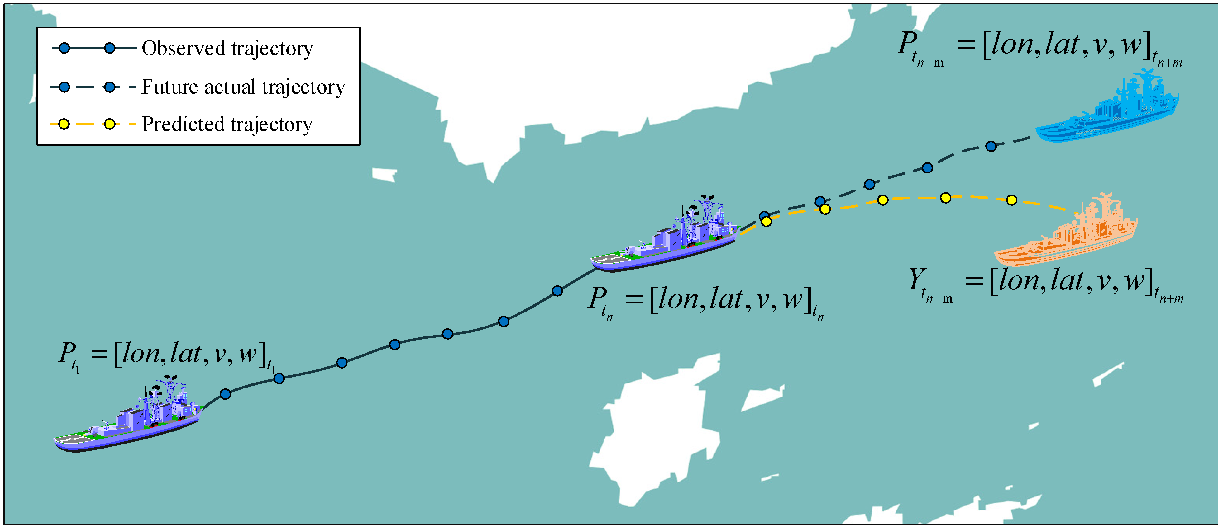
During maritime navigation, ships can observe the navigation status of surrounding vessels via AIS. This paper utilizes the maritime mobile service identity (MMSI) as a unique index for ship AIS data. It defines as the entirety of a ship’s trajectory, thereby deriving a discrete time series definition for ship trajectories, as indicated in Equation (1).
In this context, signifies the MMSI number, denotes a segment of the trajectory, and refers to the position point corresponding to the timestamp . It is composed of a four-dimensional feature vector defined by Equation (2).
Within this framework, represents longitude, denotes latitude, v signifies the ship’s speed over ground, and encapsulates the vessel’s course over ground.
The schematic illustration of ship trajectory prediction, as depicted in Figure 1, entails designating the vessel’s state information from time to as the input for the prediction model. The position data at moment are then used as the model’s output, as delineated in Equation (3).
In this model, represents the predictive function for the vessel’s trajectory obtained through our model. signifies the predicted ship state information at moment .
3.2. Design of the Vessel Trajectory Prediction Algorithm Model
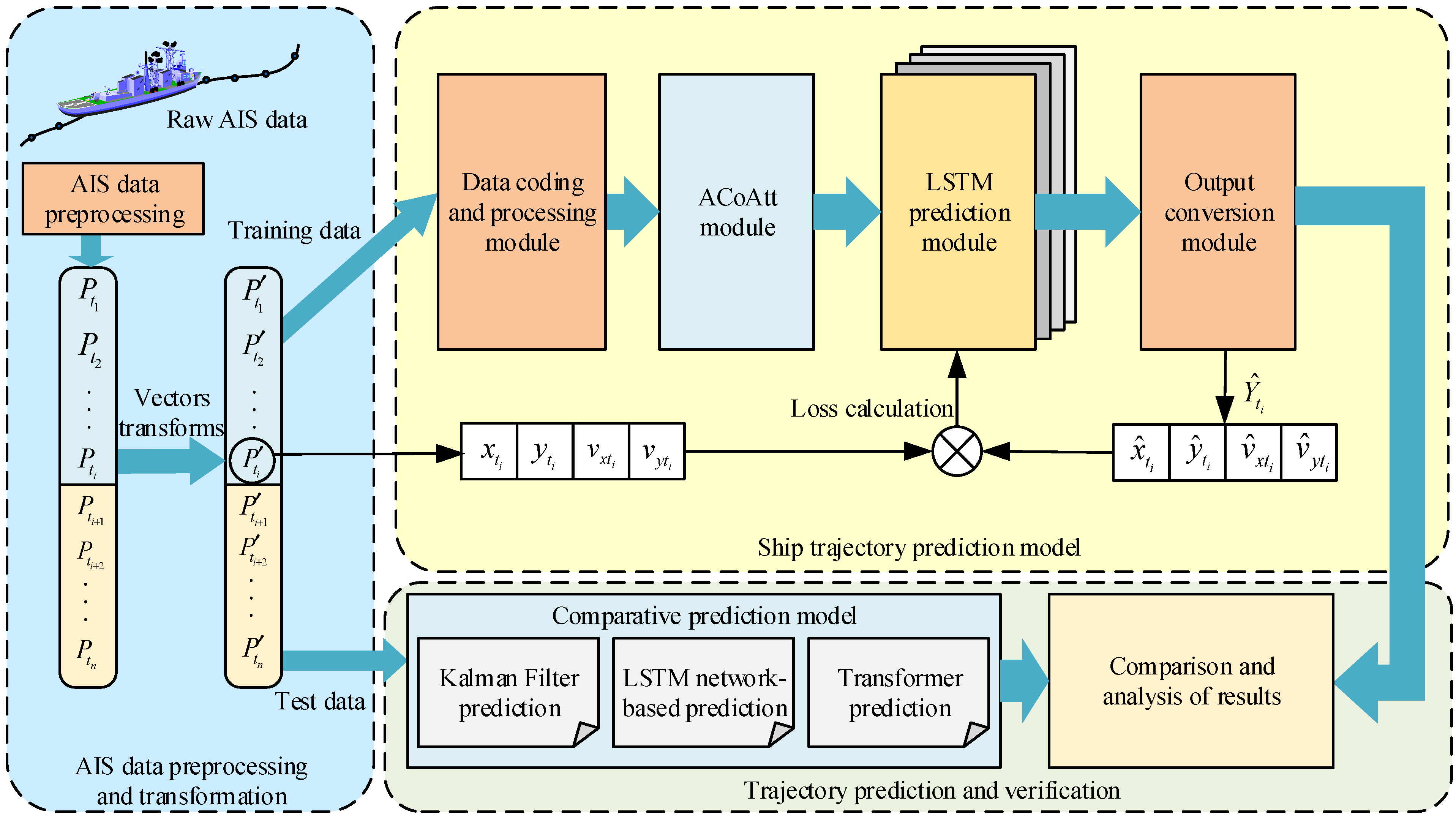
Addressing the challenge of short-term vessel trajectory prediction, our research introduces an innovative predictive model structure. This model harmoniously integrates binary code representation, ACoAtt mechanism, and LSTM networks for processing AIS data to accurately forecast future maritime trajectories. As depicted in Figure 2, the model consists of three primary modules, each offering solutions to different challenges encountered in the trajectory prediction process.
Initially, the AIS data processing module applies binary encoding to the raw AIS data, transforming continuous numerical attributes into efficient binary formats. This not only simplifies the data but also retains crucial information vital for model training, enhancing the input format’s dimensionality and efficiency. The binary encoding retains key data features and offers an effective format for deep learning models. The ACoAtt module, utilizing multi-head attention mechanisms, captures complex relationships between dynamic navigational characteristics like speed and direction changes. The ACoAtt module focuses on significant positional changes within the prediction sequence, greatly enhancing the model’s understanding of latent temporal patterns. The model integrates multi-level LSTM networks, effectively modeling dependencies in AIS data and excelling in processing spatial semantics and temporal dependencies. The predictive output conversion module is tasked with receiving the forecasted trajectory, transforming the binary representation of the trajectory prediction through a decoding process into scalar attributes, aligning them with real-world coordinates or the standard formats required by navigational systems. This supports accurate short-term vessel trajectory prediction and optimizes model parameters through backpropagation of the error calculated between predicted and actual values. Finally, the model’s reliability and effectiveness are tested in practical applications.
3.3. Preprocessing and Transformation of AIS Data
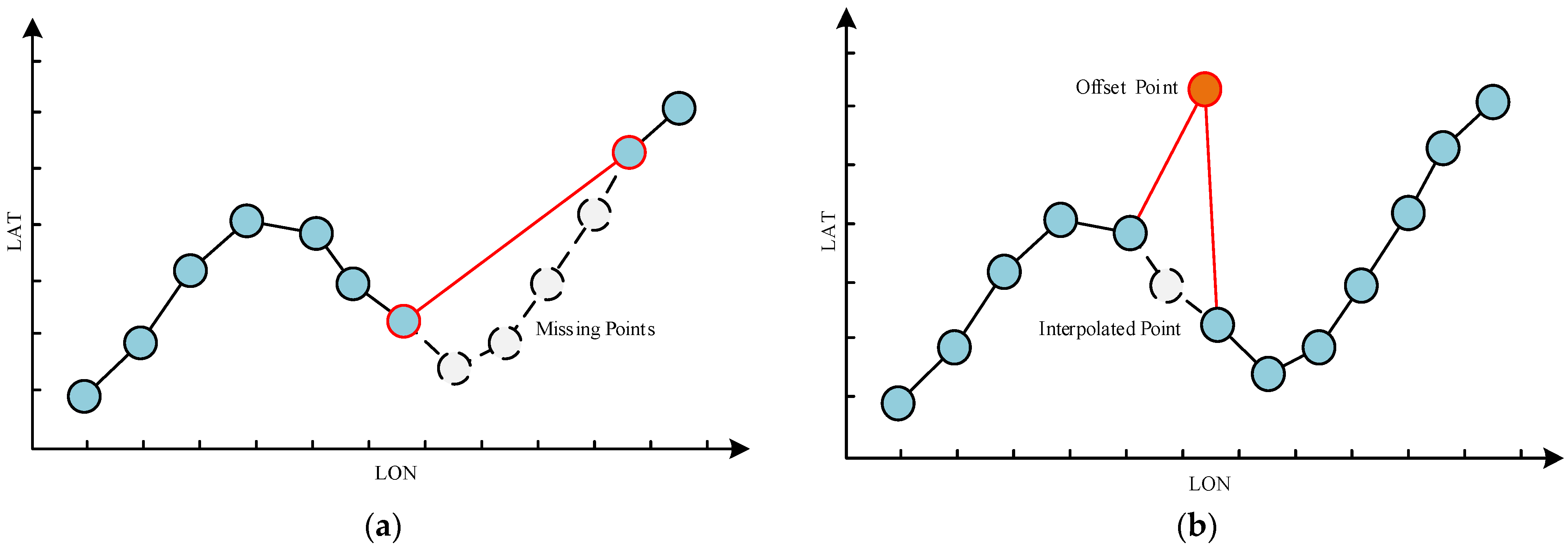
Data preprocessing aims to eliminate any anomalous data to mitigate their impact on subsequent trajectory modeling. For AIS data of vessels uniquely identified by MMSI, handling missing or aberrant data is crucial [30], as illustrated in Figure 3. This processing ensures the accuracy of data fed into the trajectory prediction model. For mathematical modeling and computational convenience, converting latitude and longitude into two-dimensional plane coordinates simplifies the model’s handling of the Earth’s curvature complexity. This simplification, particularly in short-range predictions, hardly affects the predictive accuracy.
3.3.1. Imputation Procedures for Missing AIS Data Values
Let represent the time interval between two consecutive timestamps and . In this study, if the interval exceeds 20 min, it is inferred that a data gap exists between points and , necessitating missing value imputation. The number of missing values requiring imputation is defined as:
Upon determining the quantity of missing values requiring interpolation, this study employs a bidirectional weighted-average interpolation method for latitude and longitude imputation. This approach considers the vessel’s speed and direction during the missing period, in conjunction with the current acceleration of the ship, to simulate its actual motion. It calculates the distance traveled and the direction of travel over a short period, thereby determining the position at the time of interpolation, which in turn yields the latitude and longitude coordinates of the missing data.
Assuming a section of AIS data sequence with missing values, where endpoints are designated as and , and given that endpoint ’s current ground speed, direction, and acceleration are known, their latitude and longitude coordinates can be projected onto a plane. In the bidirectional weighted interpolation for latitude and longitude, the number of missing values to be interpolated is . The Lagrange interpolation method calculates interpolated speed and direction. Forward Lagrange interpolation yields the ground speed sequence and direction from to , while interpolating missing values and speed to determine acceleration . Similarly, from to , ground speed sequence , direction , and acceleration are determined.
At this juncture, it is presumed that the vessel progresses along its current ground course , advancing at speed for a duration , arriving at the initial interpolation point. Consequently, the plane coordinates for the first missing value are:
Once the initial missing value is determined by this method, it can be treated as a new endpoint to recursively determine the coordinates of the next missing value. This process is repeated to calculate all missing values. The formula for recursively solving the coordinates of missing values is as follows, where .
Concurrently, it is imperative to correct for missing values in reverse order. The plane coordinates for these missing values are as follows, where .
By employing a bidirectional calculation, the method obtains different sequences of missing values from varying starting points. These sequences are then merged, assigning distinct weights to them. The bidirectional weighted interpolation assigns varying weights based on the time difference between the missing values and endpoints and . Greater weight is allocated when the time difference with an endpoint is smaller. The formula for the distribution of weights and is as follows:
The coordinates calculated through the weighted average method are the longitudinal and latitudinal values sought for the missing data, and . The values for these coordinates are as follows:
3.3.2. AIS Data Deviations
For significantly deviated trajectory points, they are considered as missing values, and methods for missing value imputation are employed to address these anomalies. By comparing a ship’s trajectory point with its adjacent points, the deviated trajectory points are identified. If the distance between the current trajectory point and its neighboring points and is substantially different, exceeding a predefined threshold, then point is deemed a trajectory deviation point.
Moreover, by calculating the average speed between a drift point and its adjacent trajectory points, based on their distance and time interval, erroneous data can be detected. If the computed average speed exceeds the vessel’s maximum speed, the trajectory point is deemed erroneous. The specific formula for this determination is outlined in Equation (10).
where represents the maximum speed of the target vessel, drift point is determined and subjected to mean value interpolation. The interpolated data point at time , calculated using the trajectory points adjacent to the drift point, is computed as shown in Equation (11).
3.3.3. Vector Transformation
Transforming a ship’s AIS data into position and velocity coordinates within a two-dimensional plane is a crucial process for trajectory prediction models. This transformation geometrizes geographical location data, making them more suitable for mathematical manipulation and model application. Such conversions aid in intuitively representing and analyzing trajectories on a two-dimensional plane, allowing prediction models to uncover and learn the intricate dynamics of ship behavior from extensive data. This approach significantly enhances the precision and efficiency of forecasting future ship positions.
Given the Earth’s approximation as an oblate spheroid, for the sake of simplicity in calculations, it is conventionally regarded as a sphere. We typically employ cartographic projection techniques to transform latitude and longitude into a planar coordinate system. A prevalent method utilized is the Mercator projection [31], particularly suitable for navigation within smaller regions, the equations of which are as follows:
where represents the Earth’s radius, is the reference longitude, and is the reference latitude, both measured in degrees. To reduce the data bit length and thereby simplify computational complexity, this paper selects the latitude and longitude of the first position point in the test data as the reference coordinates.
3.4. AIS Data Encoding Process
In contemporary ship trajectory prediction methods, a five-dimensional vector typically represents a ship’s position and state, including longitude, latitude, speed, direction, and time. The high dimensionality and complexity of raw AIS data make processing and analysis challenging, especially without appropriate feature engineering. This complexity can obscure the temporal and spatial relationships in the data, making it difficult to extract implicit semantic features of trajectory points and sequences from low-dimensional neural network representations during model training. Therefore, proper data preprocessing and transformation techniques in AIS data-based trajectory prediction research are crucial.
Against this backdrop, this paper innovatively proposes binary encoding of AIS data. This method’s essence lies in transforming complex ship trajectory data into a more manageable and analyzable format. It aims to mitigate the influence of varying attributes and enhance the information capacity for data mining tasks, thereby effectively boosting the performance and accuracy of trajectory prediction models.
Initially, it is necessary to quantify each continuous attribute in AIS data. Quantization is a process of mapping continuous values to a finite set of symbols. In AIS data, continuous attributes like a ship’s position coordinates ( and ) and speed (velocity components , ) need to be converted into the values within a suitable numerical range. This can be achieved using a predefined quantization factor , which is represented as:
where signifies the quantification process equation. signifies the floor function. The choice of quantization factor depends on the desired level of decimal precision retention. Subsequently, the quantized values are converted into binary representation. Given a quantized attribute range of , where is the maximum absolute value of the quantized values, the number of binary encoding bits for each attribute is set as:
where represents the ceiling function. Due to the possibility of negative values in AIS data attributes, it is crucial to consider the sign while converting to binary representation. If an element value is negative, its leading bit is set to 1 to signify the negative sign, while the subsequent bits represent the binary depiction of the element’s absolute value, resulting in the binary-encoded representation of AIS data, denoted as :
where , , , and correspond to the encoded data of , , , and , respectively. By assembling the binary representations of each element, it can be viewed as an n-hot vector.
This method converts the continuous attribute values of AIS data into a format suitable for machine learning models. The binary encoding not only reduces the dimensions of the original data but also captures the significant features of the data more precisely, providing a more robust data representation for ship trajectory prediction.
3.5. The Design of Correlation Attention Mechanism
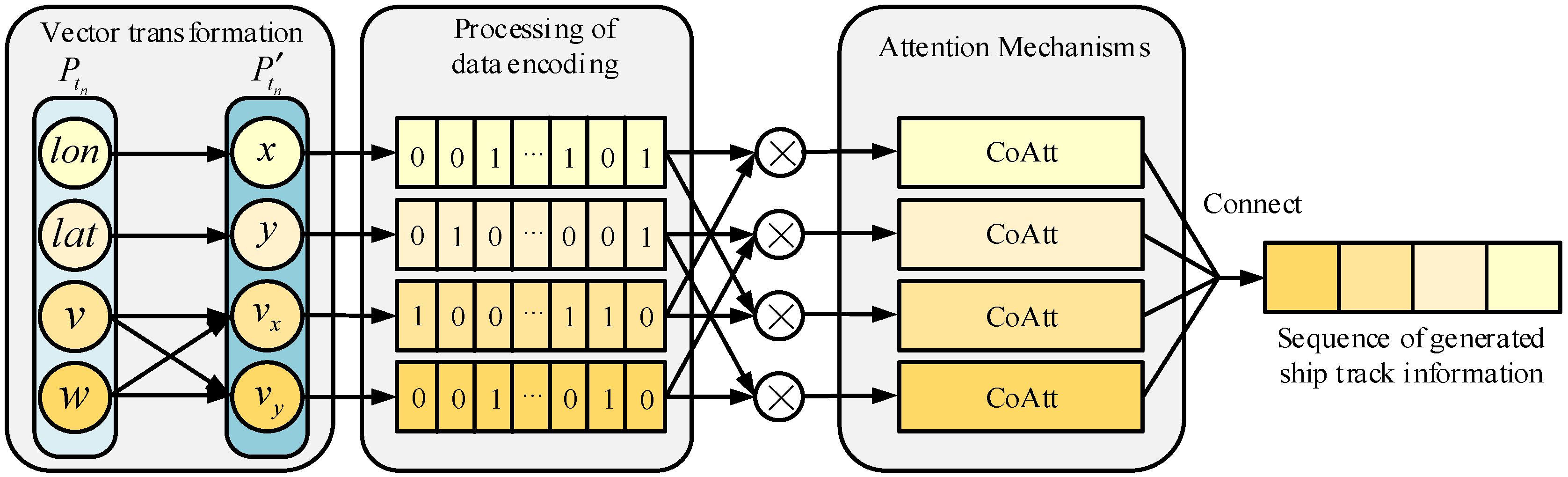
To further enhance the correlation between position and speed in ship trajectory prediction, we have delved into the design of an ACoAtt module, as depicted in Figure 4. We hypothesize that this module possesses the potential to transpose encoded data into a more condensed and highly abstracted embedding space, thereby unearthing the profound interrelations among attributes [32]. To corroborate this hypothesis, the ACoAtt design integrates a multidimensional correlation attention mechanism, dedicated to elevating the model’s proficiency in deciphering complex behavioral patterns of vessels within maritime environments. By employing several fully connected layers to funnel trajectory attributes into the model, and through the implementation of a multi-head attention mechanism, ACoAtt aspires to perform a detailed analysis and learning of the interplay among diverse attributes. Specifically, each attention head is engineered to detect the interactions among different types of attributes, with each interaction having a distinct impact on trajectory prediction. For instance, certain heads may concentrate more on dissecting the influence of velocity fluctuations on future positions, while others investigate the repercussions of temporal intervals on speed and directional alterations. This strategic approach enables the model to contemplate multiple factors in forecasting future trajectories, theoretically advancing the precision of predictions.
In practical applications, the ACoAtt module initially calculates the self-attention weights for each attribute embedding, subsequently leveraging these weights to augment the embeddings, thereby accentuating the attributes most pertinent to the current moment. Notably, distinct CoAtt modules are designed to recalibrate the embeddings of each ship trajectory attribute independently. The interplay between and , as well as and , is orchestrated in a manner that fosters mutual influence, with each module addressing different dimensions of attribute relationships and data characteristics.
Initially, the binary-encoded data are transformed into attribute-embedding vectors by mapping them through a fully connected layer into the embedding space. This transformation can be articulated using the following equation:
where represents the weight matrix of the fully connected layer, and signifies the bias element.
Subsequently, in the embedding space, the attribute-embedding vectors are processed through a multi-head attention mechanism, involving three primary steps: initially, the generation of Query (Q), Key (K), and Value (V) vectors.
where , , and represent respective weight matrices. Following this, the attention weights are calculated.
In the formula, represents the dimension of the key vector, and the function is utilized to normalize the weights. Finally, these weights are applied to the value V to obtain the final output.
The CoAtt module is ingeniously designed to intricately parse the interrelations between different navigational attributes, particularly between the ship’s position and speed. Leveraging the dynamics of prior knowledge, it is presumed that changes in position are closely linked to the preceding velocity. This module enables the model to not only capture the unique features of each attribute but also to comprehend how these attributes evolve over time in unison, thereby enhancing the accuracy of future position predictions for the ship.
3.6. LSTM Prediction Network
Building upon the encoding and ACoAtt module discussed in previous chapters, the LSTM Prediction Network section is dedicated to employing the capabilities of Long Short-Term Memory networks for processing and predicting time series in AIS data of ships. Renowned for its proficiency in handling sequential data, the LSTM network is ideally suited for the task of predicting ship trajectories. This section focuses on the implementation of a multi-layered LSTM structure to model temporal dependencies in ship trajectories, thereby forecasting their future positions.
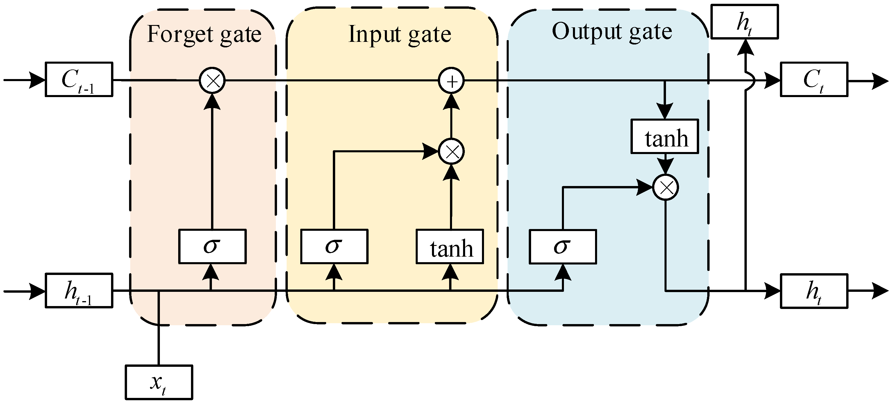
LSTM is a specialized form of RNN and excels at learning long-term dependencies within sequence data. A typical LSTM unit, as depicted in Figure 5, comprises a storage cell that maintains its state over time and three nonlinear “regulators” or gates that control the flow of information within the unit.
In this diagram, and represent the hidden state and cell state at time step , respectively. The cell state retains information learned from previous time steps. Information can be added to or removed from the cell state using these gates: the input gate (i), the forget gate (f), and the output gate (o). At each time step , the module uses the past state of the network ( and ) and the input to compute the output and the updated cell state . The hidden state and cell state are recurrently connected back to the block input. All gates are controlled by the hidden state from the previous cycle and the input vector . Most modern research incorporates many improvements made since the initial proposal of the LSTM architecture. The mathematical expressions for each gate of the LSTM can be formulated as follows:
where and represent the weight matrices and bias terms, respectively. denotes the sigmoid function. is the hidden state from the previous time step, while is the input at the current time step. The newly generated information and the cell state at the current time step are given by:
In the formula, represents the hyperbolic tangent function. Based on the mathematical expressions for each gate of the LSTM unit as per Equations (19) and (20), the output function of the LSTM unit can be represented as follows:
4. Experimental Validation
In this study, we developed an innovative method for predicting ship trajectories by combining data encoding transformation, the ACoAtt module, and LSTM networks. This approach aimed to validate the effectiveness, reliability, and real-time capabilities of the proposed algorithm through various simulation experiments, followed by in-depth discussion and analysis of the results.
4.1. Description of Experimental Data
The study utilized publicly available AIS data from the Marinecadastre website, focusing on segments of ship trajectories from 2022 for experimental analysis. We conducted a comprehensive analysis using the navigational trajectory data of 42 vessels, with the dataset featuring an average of 874 AIS data points per vessel. These trajectories span multiple maritime areas and encompass a broad spectrum of environmental conditions, aiming to thoroughly evaluate the performance of our proposed model across diverse scenarios. The trajectories of six ships in six different regions, as depicted in Table 1, represent merely a fraction of our experimental dataset.
The selected AIS data encompassed details like ship identification numbers (MMSI), longitude, latitude, speed over ground (SOG), and course over ground (COG). To ensure precise experimental prediction outcomes, longitude and latitude were recorded to five decimal places, equating to roughly 1 m accuracy. Speed was measured in knots with one decimal place accuracy, while the course was recorded in degrees, also with one decimal place precision. A sample of these trajectories is presented in Table 2.
To thoroughly evaluate the performance of the proposed model, we segmented the trajectory prediction dataset, adopting an 8:2 ratio to bifurcate the dataset into a training set and a testing set. Specifically, 80% of the data were designated as the training set, dedicated to the model’s learning and optimization processes, while the remaining 20% were allocated to the testing set, intended for subsequent performance evaluation and verification. Within the testing set, we deliberately selected data encompassing linear and maneuvering trajectory patterns, to conduct an in-depth analysis of the model’s accuracy and robustness in handling diverse navigational behaviors.
4.2. Design of Experimental Evaluation Indicators
When evaluating the accuracy of the predictive model used, it is essential to consider the discrepancy between the predicted results and the actual values due to various factors. The study employs three metrics for assessing the model’s performance: mean absolute error (MAE), root-mean-square error (RMSE), and hit rate. These metrics provide a comprehensive evaluation of the model’s predictive accuracy and reliability.
where represents the actual values of the ship’s navigational data, while denotes the predicted estimates of the ship’s trajectory data. refers to the number of AIS data samples used for testing purposes.
In this study, the prediction of a ship’s navigational trajectory is conducted by forecasting individual trajectory points. The hit rate serves as an intuitive indicator of the model’s precision in predicting these trajectory points. A prediction is considered accurate when the distance between the forecasted and actual points is relatively close. To calculate the hit rate, the first step involves computing the straight-line distance between the actual and predicted trajectory points.
In this context, and denote the predicted latitude and longitude coordinates, respectively, while and represent the actual latitude and longitude coordinates. R signifies the Earth’s radius, measured in kilometers.
A threshold for maximum prediction error , measured in meters, is established. If the distance between the predicted and actual points is less than , the prediction is considered accurate, a “hit”. If exceeds , it is a “miss”, indicating a failed prediction. The hit rate, representing the success rate of accurate predictions, is calculated as the number of hits divided by the total number of predictions .
In the ship trajectory prediction experiments of this section, a larger value of indicates a smaller difference between the predicted value and the actual value, signifying higher prediction accuracy. Conversely, smaller values of and indicate that the predictions are closer to the actual data, further illustrating the precision of the predictive model.
4.3. Comparison of Experimental Prediction Methods
To evaluate the proposed ship trajectory prediction framework, three comparative prediction methods were designed for the experiments:
(1) Kalman Filter prediction model: The Kalman Filter (KF) algorithm involves two processes: time updating (prediction) and measurement updating (correction). The prediction process uses the values determined at any given moment for prior estimation, and then estimates the next moment. The measurement update process corrects the model using measured values, offering a posterior estimate improved from the current state. To ensure the accuracy and effectiveness of the KF algorithm, it has been extended in this study to adapt to the dynamic characteristics of ship movement. The state vector is defined to include position (longitude and latitude), speed, acceleration, and rate of turn.
(2) LSTM network-based prediction model: The ability of LSTM networks is particularly suitable for processing time series in ship AIS data, as these often contain complex spatiotemporal patterns and dynamics. Through training, LSTM networks can learn patterns extracted from historical data and use these to accurately predict future ship positions and behaviors. Furthermore, comparing the LSTM network with the prediction framework proposed in this study allows for the validation of the effectiveness of the associative attention mechanism introduced in the paper.
(3) Transformer-based time series forecasting: Since its inception, the surge in Transformer-based solutions for time series forecasting tasks has been noteworthy [33]. Transformers, with their adeptness at extracting semantic correlations among elements within extensive sequences, boast remarkable capabilities in parallel sequence processing, rendering them highly suitable for modeling time series characterized by pronounced periodicity and elongated sequence lengths. This model, reliant on the parallel processing of self-attention mechanisms, facilitates the effortless extraction of relationships between temporally distant steps within a sequence.
The proposed prediction model in the paper is configured as follows: After vector transformation of AIS data elements, 18-bit binary encoding is used to represent positions in the and directions, and 10-bit binary encoding is used for speeds in these directions, with the highest bit indicating the sign of the value. The correlation attention mechanism module uses four multi-head attention operators. In the LSTM main prediction network part, six stacked LSTM networks are set as the main model, with each LSTM layer having a count of three. The number of hidden units per layer ranges from 32 to 256. The training simulation is run for 500 iterations using the Adam adaptive learning rate optimization algorithm, with an initial learning rate of 0.2. To prevent model overfitting, L2 regularization is adjusted with a coefficient set at 0.01.
4.4. Results and Analysis
For the test experiments of the model, the following hardware conditions were used: The operating system was Windows 10, the CPU was an Intel® i7-11700F, which produced by Intel Corporation in Santa Clara, CA, USA, and the GPU was an NVIDIA GeForce GTX 1080Ti, manufactured by NVIDIA Corporation located in Santa Clara, CA, USA. The programming language used was Python 3.8, and the deep learning framework utilized was PyTorch 2.0.
4.4.1. Comparison of Different Types of Trajectory Predictions
This experiment compares various trajectory prediction models, including the Kalman Filter prediction model, LSTM-based prediction model, Transformer prediction model, and the model proposed in this study, for different types of trajectories such as straight-line navigation and turning maneuvers. The first 30 moments of ship navigation trajectory points are used as inputs for the models, predicting the trajectories for the subsequent 10 sampling time points, which corresponds to approximately 12 min of trajectory prediction.
- (1)
- Straight-line navigation
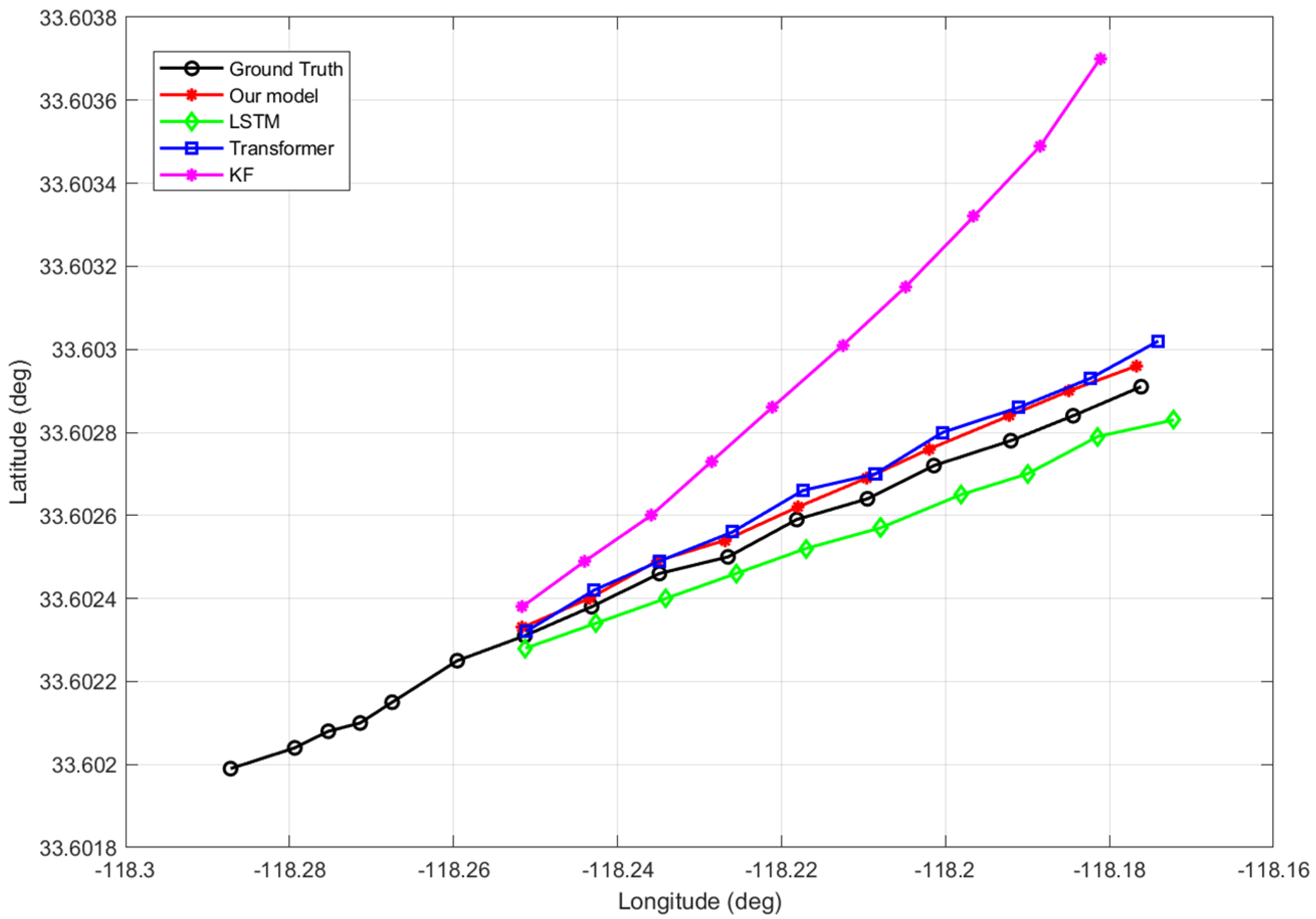
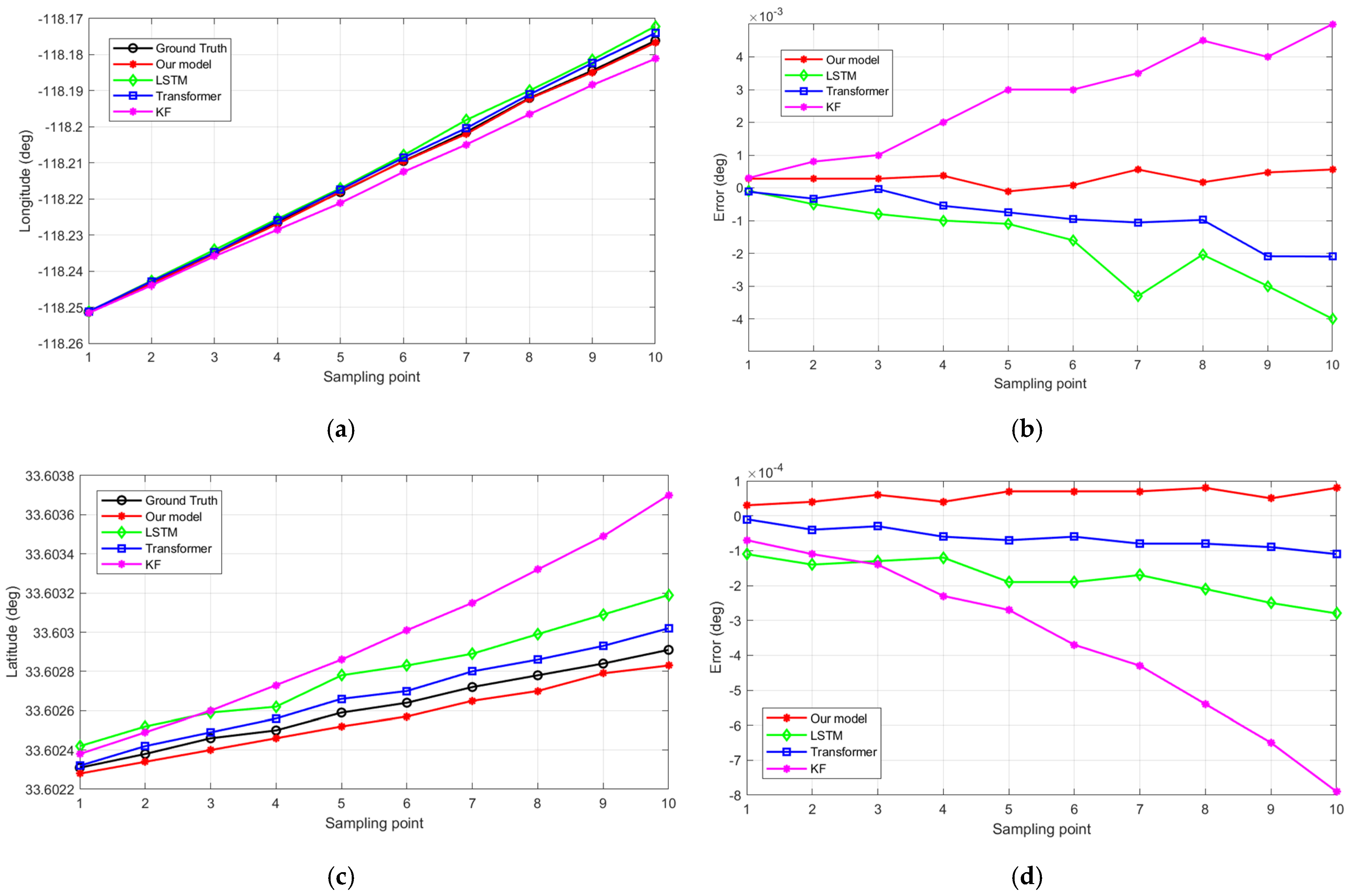
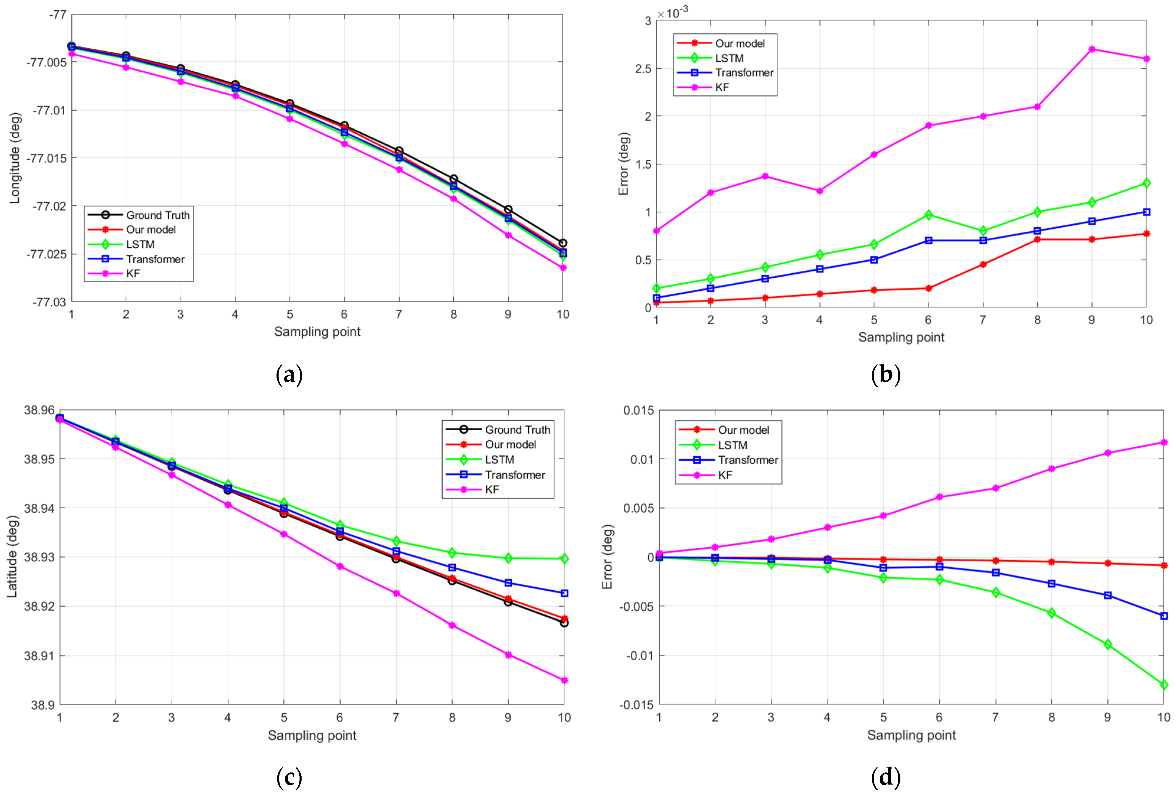
In the case of straight-line navigation, the real trajectory involved sailing in a nearly straight line with a course of about 89.7° and a speed of around 10 knots. The target ship started sailing along a planned route, maintaining relatively stable direction and speed. Trajectory predictions were made using different methods starting from the 7th point in the trajectory. A comparison of the predictions from these various methods is illustrated in Figure 6. An error analysis was performed on the latitude and longitude predictions from different methods at the same forecast point. This analysis provided a comparison of the latitudinal and longitudinal predictions and their errors for each method, as depicted in Figure 7.
- (2)
- Curved maneuver navigation
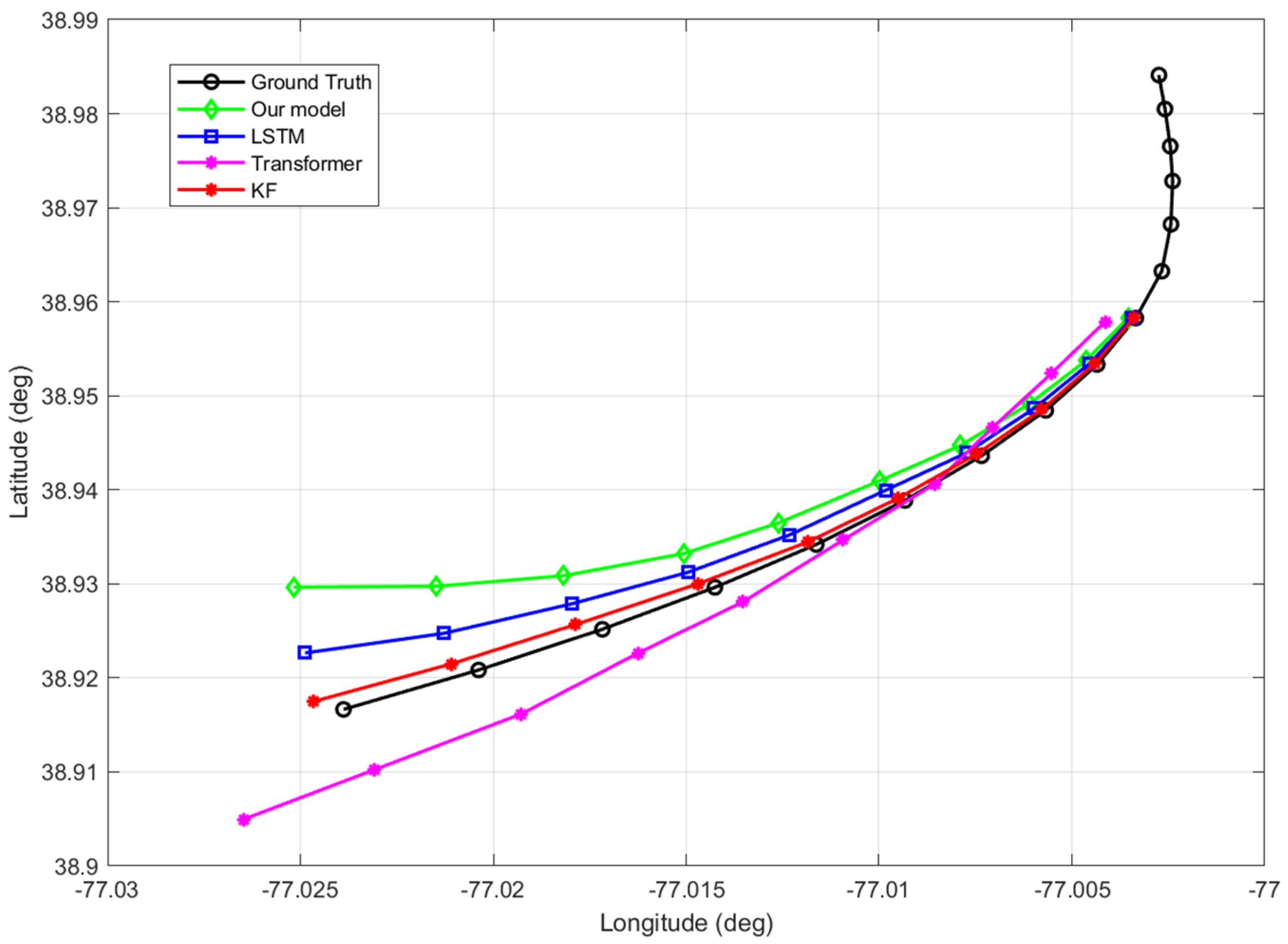
The real trajectory involved curved maneuvering, starting at a course of approximately 175° and ending at about 262°. The initial speed was around 9 knots, slowing down and then speeding up during the turn, ending at approximately 12 knots. Similar to the previous case, at the 7th point in the chart, different methods were used to predict the trajectory. The comparative results of these different prediction methods are illustrated in Figure 8. The study also conducted an error analysis on the latitude and longitude predictions for different prediction points, comparing the results and errors of each prediction method. This comparison and error analysis are depicted in Figure 9.
The paper conducted a comprehensive analysis of simulation results, comparing the longitude and latitude prediction errors of four models. It also calculated key performance metrics for each model, including average absolute error, root-mean-square error, and prediction hit rate. The performance analysis of the proposed model and the other three models is detailed in Table 3. We set a maximum prediction error of 150 m as a benchmark to assess the prediction hit rates of the various algorithms.
The study’s model exhibited superior predictive performance in both linear and curvilinear ship trajectory prediction compared to the KF model, LSTM-based model, and Transformer model. It achieved the lowest root-mean-square error, average absolute error, and hit rate across different scenarios, outperforming other models, especially in linear prediction scenarios where the KF model showed significant errors. The Transformer model followed in effectiveness, with the multi-layer LSTM model next in line. This highlights the advanced predictive capability of the proposed model over traditional and other intelligent prediction methods. Furthermore, the study’s model, alongside LSTM-based and Transformer models, showed similar patterns of increasing prediction errors with longer prediction steps. While the initial prediction errors were marginally different, the root-mean-square errors varied significantly among the models. In curvilinear motion prediction, the study’s model exhibited markedly lower root-mean-square errors in both latitude and longitude (0.000437 and 0.000411, respectively) compared to other methods. This indicates the model’s superior predictive performance over traditional KF predictions and other intelligent algorithms.
On the other hand, by contrasting the predictive outcomes and statistics of our model with those of the multi-layer LSTM network, our approach demonstrates superior accuracy in predicting various feature attributes in both scenarios. Specifically, in straight-line navigation, there is a notable reduction in the mean absolute error (MAE) for latitude and longitude predictions, and a similar trend is observed in curvilinear motion scenarios. Additionally, our model shows greater stability for longer prediction intervals compared to the multi-layer LSTM model. The results validate the efficacy of the proposed ACoAtt, effectively integrating historical trajectory and current state information to uncover hidden inter-sequential information. This approach distinctly captures the feature interrelations post binary encoding, demonstrating that the proposed model architecture significantly enhances the accuracy of ship trajectory prediction.
4.4.2. Comparison of Multi-Step Trajectory Prediction
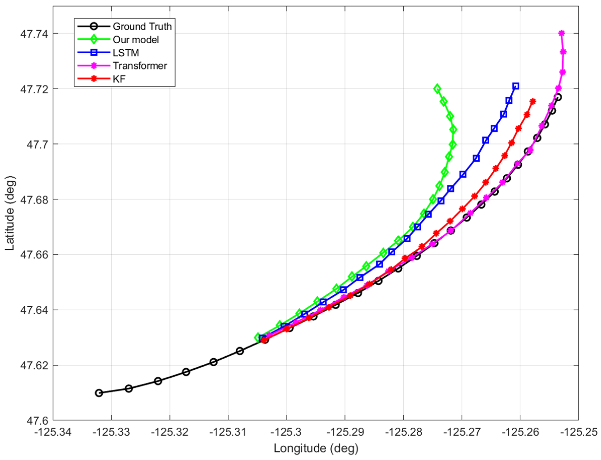
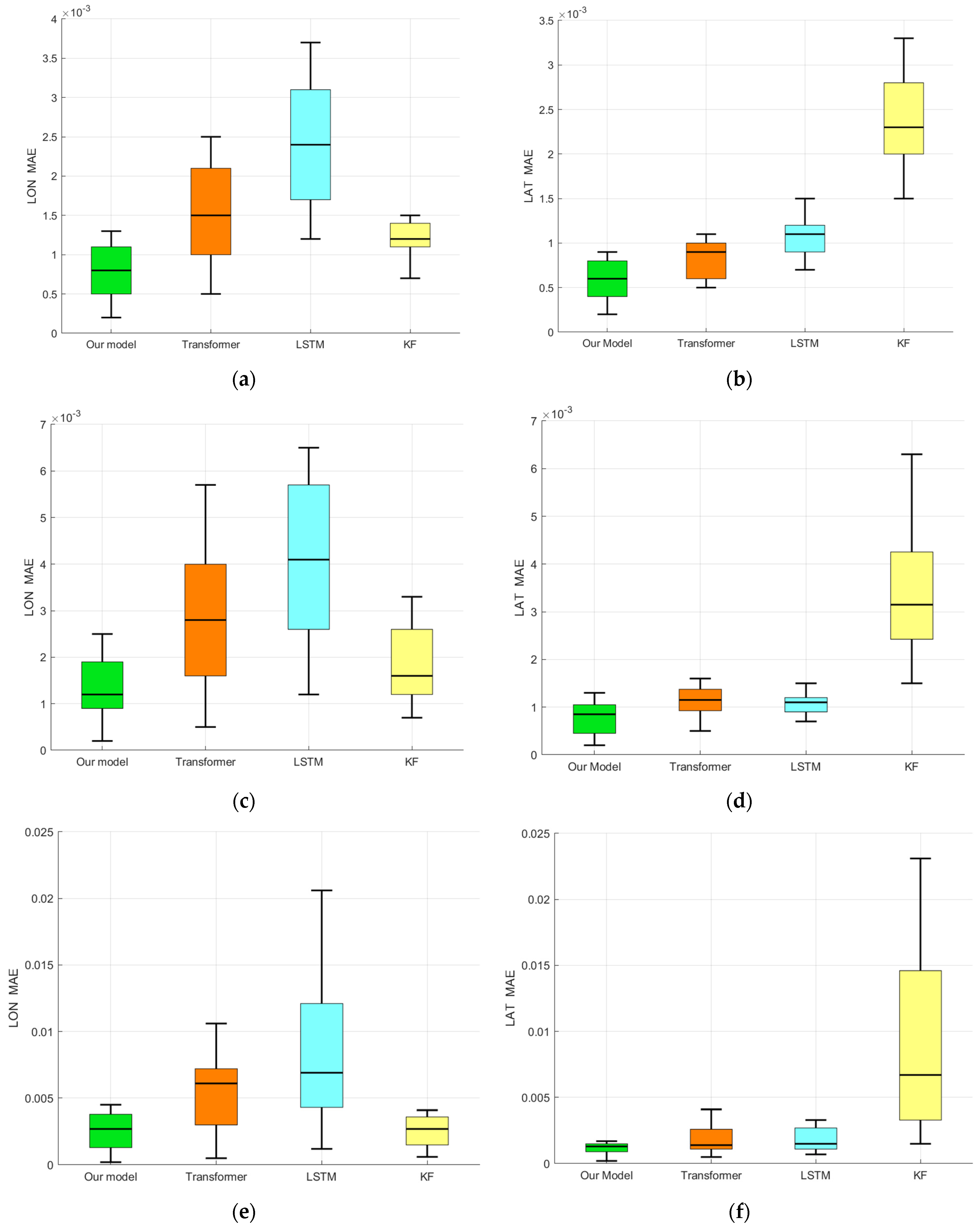
To assess the robustness and stability of the proposed method across varying prediction lengths, this section opts for a test set comprising navigational trajectories under curvilinear maneuvering conditions. Predictions are made for ship trajectory points at 5, 10, and 20 moments in time, corresponding to approximate durations of 6 min 30 s, 13 min, and 26 min, respectively. This approach serves to validate the testing model’s performance in short-to-medium-term ship trajectory forecasting.
The real trajectory of the ship involved curve maneuvering, starting at an initial course of about 83°, ending around 27°, with an initial speed of about 11 knots, decreasing during the turn, and ending at about 9 knots. Predictions began from the seventh point in the trajectory, and the comparative results of different prediction methods are shown in Figure 10.
To further assess the impact of step length on ship trajectory prediction tasks, the MAE of different prediction methods at 5, 10, and 20 moments was statistically analyzed. Box plots were used to display the MAE of latitude and longitude attributes, as shown in Figure 11. Additionally, the average RMSE of the four models at different prediction lengths is depicted in Table 4.
The statistical analysis of the experimental simulation results for predicting ship trajectories over consecutive 5, 10, and 20 moments is outlined in Table 4.
Commencing with an analysis grounded in the visualization outcomes, an examination of predictive accuracy is undertaken. The model introduced herein achieves the pinnacle of predictive performance. Furthermore, as the prediction horizon extends, various forecasting methodologies tend to incur greater predictive discrepancies. When the trajectory point prediction length is minimal, each model can accurately forecast future trajectories within the initial four prediction steps (approximately 5 min), with the average absolute error and root-mean-square error of the four models being comparably close. This suggests that the current methodologies can adequately meet the demands for ultra-short-term trajectory forecasting, with the model presented in this paper exhibiting superior performance. However, as the number of prediction steps increases, some predicted trajectories gradually diverge from the actual scenarios, leading to a decline in trajectory forecasting precision across all four models. Yet, the rate of decline in predictive accuracy for the model discussed in this paper is significantly lower than that of the Kalman Filter prediction model, LSTM network-based prediction model, and Transformer prediction model. At a prediction length of 20 trajectory points, the average root-mean-square error is substantially lower than the other three comparative methods. This indicates that for the problem of longer continuous ship trajectory prediction, the model designed in this paper is capable of achieving commendable predictive outcomes.
Subsequently, an analysis focused on the trend-following aspect of predictions was conducted. The method proposed in this manuscript, in comparison to other models, can swiftly forecast future motion trends within several prediction steps, as depicted in Figure 10. The model presented here is capable of stably and accurately predicting ships’ curvilinear maneuvering navigation. In contrast, the Transformer model, due to its attention mechanism, can correctly predict trajectory change trends, yet its predictive accuracy falls short. The LSTM-based prediction model, on the other hand, erroneously estimates the ships’ maneuvering intent, gradually diverging from the true course in subsequent prediction steps. Kalman Filter predictions made more accurate forecasts regarding future trajectory trends in this round of testing, but the deviation between predicted points and actual trajectory points was too significant, resulting in subpar overall predictive performance.
Lastly, an analysis focusing on the stability of prediction lengths was undertaken. According to the test outcomes, the method proposed in this manuscript, alongside the Transformer model, exhibited commendable performance within the initial ten prediction steps. However, as the prediction length extended, the predictive trend gradually deviated, rendering the results unreliable. Consequently, in the realm of short-term ship trajectory prediction applications, the method introduced herein demonstrates superior stability and outperforms other comparative forecasting techniques, albeit its efficacy wanes in mid-term predictive applications.
To further evaluate the predictive capabilities of the model, we selectively extracted data from the test set, which constitutes 20% of the navigational trajectory data of 42 vessels, resulting in a total of 64 linear navigation test trajectories and 12 curvilinear maneuvering trajectories. These were subjected to tests using various predictive methods, with a prediction length set at 10 steps. The model’s forecasts were assessed based on the error between predicted and actual latitude and longitude, with a comparative statistical analysis of the outcomes from different predictive approaches, as illustrated in Table 5.
As evidenced by Table 5, our model demonstrates a general improvement across three performance evaluation metrics, both in terms of accuracy and stability. Quantitatively speaking, it achieved the best results in longitude prediction across all evaluative indicators, showcasing the highest accuracy and commendable predictive performance. The test outcomes affirm that the predictive framework proposed in this paper can effectively unearth the correlations between target feature attributes, producing highly confident predictive trajectory outcomes. It supports an extended short-term prediction process, contributing to the enhancement of maritime performance and presenting a significant advantage in trajectory prediction.
5. Conclusions
This paper introduces an innovative method for predicting ship trajectories based on AIS data. The approach combines data encoding transformation, the ACoAtt module, and LSTM networks. Data encoding effectively represents AIS data, reducing complexity while retaining key information. The ACoAtt module, using a multi-head attention mechanism, captures complex relationships between dynamic ship features, enhancing understanding of hidden time series patterns in the data. Finally, the LSTM network accurately predicts future ship trajectories by processing time series data. By testing with historical AIS datasets, the proposed method in this article has been proven to outperform classical prediction models and other latest models with attention mechanisms in trajectory prediction accuracy. It significantly enhances the performance of existing models, offering superior accuracy and stability in trajectory prediction. This research addresses challenges in ship trajectory prediction due to the complexity of ship movements, providing notable improvements in data representation efficiency, time series data processing, and dynamic feature correlation analysis. Moreover, this algorithm can also be adapted for applications in other geospatial applications.
In our future work, we intend to focus on the application of this method for ship collision avoidance, aiming to establish a new paradigm in maritime safety and further enhance the security of ship navigation. Additionally, we are exploring more effective ways to utilize historical trajectory data to predict longer step lengths in accurate trajectory distributions.
Author Contributions
Conceptualization, Bing Li and Mingze Li; methodology, Jiashuai Li and Mingze Li; software, Mingze Li and Zhigang Qi; validation, Bing Li and Mingze Li; formal analysis, Zhigang Qi and Jiashuai Li; writing—original draft preparation, Mingze Li, Bing Li, and Jiawei Wu; project administration, Jiashuai Li and Jiawei Wu; funding acquisition, Jiashuai Li and Jiawei Wu; writing—review and editing, Mingze Li, Bing Li, and Zhigang Qi. All authors have read and agreed to the published version of the manuscript.
Funding
This research was funded by the Project of Education Science Planning in Heilongjiang Province (GJB1320064) and the Harbin Engineering University Education and Teaching Programme (JG2021B06).
Data Availability Statement
The data used to support the findings of this study are included within the article and are also available from the corresponding authors upon request.
Conflicts of Interest
The authors declare no conflicts of interest.
References
- Kundakçı, B.; Nas, S.; Gucma, L. Prediction of Ship Domain on Coastal Waters by Using AIS Data. Ocean Eng. 2023, 273, 113921. [Google Scholar] [CrossRef]
- Lyu, H.; Hao, Z.; Li, J.; Li, G.; Sun, X.; Zhang, G.; Yin, Y.; Zhao, Y.; Zhang, L. Ship Autonomous Collision-Avoidance Strategies—A Comprehensive Review. J. Mar. Sci. Eng. 2023, 11, 830. [Google Scholar] [CrossRef]
- Chiang, H.-T.L.; Tapia, L. COLREG-RRT: An RRT-Based COLREGS-Compliant Motion Planner for Surface Vehicle Navigation. IEEE Robot. Autom. Lett. 2018, 3, 2024–2031. [Google Scholar] [CrossRef]
- Liu, R.W.; Liang, M.; Nie, J.; Yuan, Y.; Xiong, Z.; Yu, H.; Guizani, N. STMGCN: Mobile Edge Computing-Empowered Vessel Trajectory Prediction Using Spatio-Temporal Multigraph Convolutional Network. IEEE Trans. Ind. Inform. 2022, 18, 7977–7987. [Google Scholar] [CrossRef]
- Gao, D.; Zhu, Y.; Guedes Soares, C. Uncertainty Modelling and Dynamic Risk Assessment for Long-Sequence AIS Trajectory Based on Multivariate Gaussian Process. Reliab. Eng. Syst. Saf. 2023, 230, 108963. [Google Scholar] [CrossRef]
- Zhou, T.; Zhang, X.; Droguett, E.L.; Mosleh, A. A Generic Physics-Informed Neural Network-Based Framework for Reliability Assessment of Multi-State Systems. Reliab. Eng. Syst. Saf. 2023, 229, 108835. [Google Scholar] [CrossRef]
- Wieder, O.; Kohlbacher, S.; Kuenemann, M.; Garon, A.; Ducrot, P.; Seidel, T.; Langer, T. A Compact Review of Molecular Property Prediction with Graph Neural Networks. Drug Discov. Today Technol. 2020, 37, 1–12. [Google Scholar] [CrossRef]
- Lindemann, B.; Müller, T.; Vietz, H.; Jazdi, N.; Weyrich, M. A Survey on Long Short-Term Memory Networks for Time Series Prediction. Procedia CIRP 2021, 99, 650–655. [Google Scholar] [CrossRef]
- Zhao, L.; Zuo, Y.; Li, T.; Chen, C.L.P. Application of an Encoder–Decoder Model with Attention Mechanism for Trajectory Prediction Based on AIS Data: Case Studies from the Yangtze River of China and the Eastern Coast of the U.S. J. Mar. Sci. Eng. 2023, 11, 1530. [Google Scholar] [CrossRef]
- Gu, J.; Sun, C.; Zhao, H. DenseTNT: End-to-End Trajectory Prediction from Dense Goal Sets. In Proceedings of the IEEE/CVF International Conference on Computer Vision, Montreal, BC, Canada, 11–17 October 2021; pp. 15303–15312. [Google Scholar]
- Guo, D.; Wu, E.Q.; Wu, Y.; Zhang, J.; Law, R.; Lin, Y. FlightBERT: Binary Encoding Representation for Flight Trajectory Prediction. IEEE Trans. Intell. Transp. Syst. 2023, 24, 1828–1842. [Google Scholar] [CrossRef]
- Zhou, H.; Chen, Y.; Zhang, S. Ship Trajectory Prediction Based on BP Neural Network. J. Artif. Intell. 2019, 1, 29–36. [Google Scholar] [CrossRef]
- Murat Üney, L.M.M. Data Driven Vessel Trajectory Forecasting Using Stochastic Generative Models. In Proceedings of the ICASSP 2019—2019 IEEE International Conference on Acoustics, Speech and Signal Processing (ICASSP), Brighton, UK, 12–17 May 2019. [Google Scholar]
- Perera, L.P.; Oliveira, P.; Soares, C.G. Maritime Traffic Monitoring Based on Vessel Detection, Tracking, State Estimation, and Trajectory Prediction. IEEE Trans. Intell. Transp. Syst. 2012, 13, 1188–1200. [Google Scholar] [CrossRef]
- Jaskólski, K. Availability of Automatic Identification System (AIS) Based on Spectral Analysis of Mean Time to Repair (MTTR) Determined from Dynamic Data Age. Remote Sens. 2022, 14, 3692. [Google Scholar] [CrossRef]
- Li, J.; Zhou, L. Improved Satisfactory Predictive Control Algorithm with Fuzzy Setpoint Constraints. In Proceedings of the 2006 6th World Congress on Intelligent Control and Automation, Dalian, China, 21–23 June 2006; Volume 2, pp. 6274–6278. [Google Scholar]
- Lian, Y.; Yang, L.; Lu, L.; Sun, J.; Lu, Y. Research on Ship AIS Trajectory Estimation Based on Particle Filter Algorithm. In Proceedings of the 2019 11th International Conference on Intelligent Human-Machine Systems and Cybernetics (IHMSC), Hangzhou, China, 24–25 August 2019. [Google Scholar]
- Liao, L.; Köttig, F. Review of Hybrid Prognostics Approaches for Remaining Useful Life Prediction of Engineered Systems, and an Application to Battery Life Prediction. IEEE Trans. Reliab. 2014, 63, 191–207. [Google Scholar] [CrossRef]
- Murray, B.; Perera, L.P. A Data-Driven Approach to Vessel Trajectory Prediction for Safe Autonomous Ship Operations. In Proceedings of the 2018 Thirteenth International Conference on Digital Information Management (ICDIM), Berlin, Germany, 24–26 September 2018. [Google Scholar]
- Tan, Z.; Zhang, Z.; Xing, T.; Huang, X.; Gong, J.; Ma, J. Exploit Direction Information for Remote Ship Detection. Remote Sens. 2021, 13, 2155. [Google Scholar] [CrossRef]
- Liu, J.; Shi, G.; Zhu, K. Vessel Trajectory Prediction Model Based on AIS Sensor Data and Adaptive Chaos Differential Evolution Support Vector Regression (ACDE-SVR). Appl. Sci. 2019, 9, 2983. [Google Scholar] [CrossRef]
- Wang, C.; Zhu, M.; Osen, O.; Zhang, H.; Li, G. AIS data-based probabilistic ship route prediction. In Proceedings of the 2023 IEEE 6th Information Technology, Networking, Electronic and Automation Control Conference (ITNEC), Chongqing, China, 24–26 February 2023. [Google Scholar]
- Yang, C.H.; Wu, C.H.; Shao, J.C.; Wang, Y.C.; Hsieh, C.M. AIS-Based Intelligent Vessel Trajectory Prediction Using Bi-LSTM. IEEE Access 2022, 10, 24302–24315. [Google Scholar] [CrossRef]
- Liu, T.; Ma, J. Ship Navigation Behavior Prediction Based on AIS Data. IEEE Access 2022, 10, 47997–48008. [Google Scholar] [CrossRef]
- Yu, J.; Wang, J.; Ren, R.; Lu, H.; Lai, Q.; Luo, X. Research on Ship Trajectory Prediction Using LSTM and BP Based on AIS Data. In Proceedings of the 2022 5th International Conference on Computing and Big Data (ICCBD), Shanghai, China, 16–18 December 2022; IEEE: Piscataway, NJ, USA, 2022. [Google Scholar]
- Gao, D.; Zhu, Y.; Zhang, J.; He, Y.; Yan, K.; Yan, B. A Novel MP-LSTM Method for Ship Trajectory Prediction Based on AIS Data. Ocean Eng. 2021, 228, 108956. [Google Scholar] [CrossRef]
- Zhao, Y.; Cui, J.; Yao, G. Online Learning based GA-BP Neural Network to Predict Ship Trajectory. In Proceedings of the 2021 China Automation Congress (CAC), Beijing, China, 22–24 October 2021; IEEE: Piscataway, NJ, USA, 2021. [Google Scholar]
- Pallotta, G.; Vespe, M.; Bryan, K. Vessel Pattern Knowledge Discovery from AIS Data: A Framework for Anomaly Detection and Route Prediction. Entropy 2013, 15, 2218–2245. [Google Scholar] [CrossRef]
- Zhou, Z.; Li, T.; Zhao, Z.; Sun, C.; Chen, X.; Yan, R.; Jia, J. Time-Varying Trajectory Modeling via Dynamic Governing Network for Remaining Useful Life Prediction. Mech. Syst. Signal Process. 2023, 182, 109610. [Google Scholar] [CrossRef]
- Du, L.; Goerlandt, F.; Kujala, P. Review and Analysis of Methods for Assessing Maritime Waterway Risk Based on Non-Accident Critical Events Detected from AIS Data. Reliab. Eng. Syst. Saf. 2020, 200, 106933. [Google Scholar] [CrossRef]
- Palikaris, A.; Mavraeidopoulos, A.K. Electronic navigational charts: International standards and map projections. J. Mar. Sci. Eng. 2020, 8, 248. [Google Scholar] [CrossRef]
- Chen, T.; Rupel, J.; Mahmood, A.; Ricotta, L.; Kim, Y.; Miguel, J.S. Demo Abstract: N-Hot Weight Quantization and Approximate Multiplication for Low-Power Machine Learning. In Proceedings of the 2020 International Symposium on Low Power Electronics and Design (ISLPED), Boston, MA, USA, 10–12 August 2020. [Google Scholar]
- Feng, J.; Yang, Y.; Zhang, H.; Sun, S.; Xu, B. Path Planning and Trajectory Tracking for Autonomous Obstacle Avoidance in Automated Guided Vehicles at Automated Terminals. Axioms 2024, 13, 27. [Google Scholar] [CrossRef]
Figure 1.
Illustration of ship trajectory prediction.

Figure 2.
Proposed framework for ship trajectory prediction model.

Figure 3.
Illustrates anomalous AIS data patterns. (a) AIS data missing. (b) AIS trajectory deviations.
Figure 3.
Illustrates anomalous AIS data patterns. (a) AIS data missing. (b) AIS trajectory deviations.

Figure 4.
Schematic diagram of the correlation attention mechanism.

Figure 5.
Schematic diagram of LSTM structure.

Figure 6.
Comparative results of forecasts for straight-line routes.

Figure 7.
Comparison of prediction results and errors for straight-line routes. (a) Results in the direction of longitude. (b) Errors in the direction of longitude. (c) Results in the direction of latitudinal. (d) Errors in the direction of latitudinal.
Figure 7.
Comparison of prediction results and errors for straight-line routes. (a) Results in the direction of longitude. (b) Errors in the direction of longitude. (c) Results in the direction of latitudinal. (d) Errors in the direction of latitudinal.

Figure 8.
Comparative results of curvilinear maneuvering trajectory predictions.

Figure 9.
Comparison of prediction results and errors for curved maneuver routes. (a) Comparison of predictive outcomes in longitude. (b) Contrast of predictive errors in longitude. (c) Comparison of predictive outcomes in latitude. (d) Contrast of predictive errors in latitude.
Figure 9.
Comparison of prediction results and errors for curved maneuver routes. (a) Comparison of predictive outcomes in longitude. (b) Contrast of predictive errors in longitude. (c) Comparison of predictive outcomes in latitude. (d) Contrast of predictive errors in latitude.

Figure 10.
Comparative results of multi-step prediction.

Figure 11.
Box plots of errors for different prediction step sizes. (a) Prediction error in longitude for length of 5 steps. (b) Prediction error in latitude for length of 5 steps. (c) Prediction error in longitude for length of 10 steps. (d) Prediction error in latitude for length of 10 steps. (e) Prediction error in longitude for length of 20 steps. (f) Prediction error in latitude for length of 20 steps.


Table 1.
Experimental data of ship trajectories.
| Area | MMSI | Date | Number of Track Points |
|---|---|---|---|
| Pacific Coast Gulf of California | 636014430 | 9 December 2022 | 433 |
| Atlantic Coast Chesapeake Bay | 368172430 | 11 January 2023 | 764 |
| Atlantic Coast Narragansett Bay | 316026694 | 6 November 2022 | 1406 |
| Northern Gulf of Mexico | 368052580 | 17 December 2022 | 1244 |
| Atlantic Coast East Coast of US | 311015600 | 1 February 2023 | 719 |
| Pacific Coast Gulf of California | 3695801480 | 17 December 2022 | 847 |
Table 2.
Sample AIS data for ship trajectories.
| MMSI | Base Date Time | LON (deg) | LAT (deg) | SOG (kn) | COG (deg) |
|---|---|---|---|---|---|
| 636014430 | 9 December 2022 T02:08:05 | −118.28719 | 33.60199 | 10.2 | 89.8 |
| 636014430 | 9 December 2022 T02:10:24 | −118.27936 | 33.60204 | 10.2 | 89.9 |
| 636014430 | 9 December 2022 T02:11:36 | −118.27527 | 33.60208 | 10.0 | 89.7 |
| 636014430 | 9 December 2022 T02:12:45 | −118.27138 | 33.60209 | 10.1 | 89.0 |
| 636014430 | 9 December 2022 T02:13:55 | −118.26748 | 33.60213 | 10.1 | 90.1 |
| 636014430 | 9 December 2022 T02:16:14 | −118.25954 | 33.60225 | 10.4 | 89.2 |
Table 3.
Results of various prediction algorithms under different scenarios.
| Trajectory Situation | Model | Position | MAE | RMSE | Hit Rate |
|---|---|---|---|---|---|
| Straight-line routes | Our model | LON | 0.00032 | 0.000356 | 0.90 |
| LAT | 0.00006 | 0.000061 | |||
| LSTM | LON | 0.00174 | 0.002140 | 0.70 | |
| LAT | 0.00018 | 0.000187 | |||
| Transformer | LON | 0.00090 | 0.001130 | 0.90 | |
| LAT | 0.00006 | 0.000069 | |||
| KF | LON | 0.00271 | 0.003118 | 0.20 | |
| LAT | 0.00036 | 0.000427 | |||
| Curved maneuver route | Our model | LON | 0.00034 | 0.000437 | 0.90 |
| LAT | 0.00032 | 0.000411 | |||
| LSTM | LON | 0.00073 | 0.000808 | 0.60 | |
| LAT | 0.00378 | 0.005525 | |||
| Transformer | LON | 0.00056 | 0.000631 | 0.70 | |
| LAT | 0.00169 | 0.002518 | |||
| KF | LON | 0.00175 | 0.001846 | 0.60 | |
| LAT | 0.00548 | 0.006690 |
Table 4.
Statistics on the predictions of the four models at different prediction lengths.
| Prediction Length | Model | Position | MAE | RMSE | Hit Rate |
|---|---|---|---|---|---|
| 5 | Our model | LON | 0.00078 | 0.00088 | 1.00 |
| LAT | 0.00058 | 0.00063 | |||
| LSTM | LON | 0.00242 | 0.00258 | 1.00 | |
| LAT | 0.00108 | 0.00111 | |||
| Transformer | LON | 0.00152 | 0.00168 | 1.00 | |
| LAT | 0.00082 | 0.00085 | |||
| KF | LON | 0.00118 | 0.00121 | 1.00 | |
| LAT | 0.00228 | 0.00233 | |||
| 10 | Our model | LON | 0.00132 | 0.00149 | 1.00 |
| LAT | 0.00077 | 0.00084 | |||
| LSTM | LON | 0.00406 | 0.00445 | 0.70 | |
| LAT | 0.00109 | 0.00112 | |||
| Transformer | LON | 0.00287 | 0.00328 | 0.90 | |
| LAT | 0.00111 | 0.00116 | |||
| KF | LON | 0.00187 | 0.00204 | 0.80 | |
| LAT | 0.00339 | 0.00365 | |||
| 20 | Our model | LON | 0.00258 | 0.00293 | 0.85 |
| LAT | 0.00114 | 0.00122 | |||
| LSTM | LON | 0.00853 | 0.01015 | 0.40 | |
| LAT | 0.00184 | 0.00203 | |||
| Transformer | LON | 0.00502 | 0.00558 | 0.50 | |
| LAT | 0.00193 | 0.00222 | |||
| KF | LON | 0.00454 | 0.00323 | 0.35 | |
| LAT | 0.00907 | 0.01140 |
Table 5.
Repetitive verification results statistics.
| Trajectory Situation | Model | Position | MAE | RMSE | Hit Rate |
|---|---|---|---|---|---|
| Straight-line routes | Our model | LON | 0.00094 | 0.000612 | 0.92 |
| LAT | 0.00091 | 0.000554 | |||
| LSTM | LON | 0.00254 | 0.002845 | 0.82 | |
| LAT | 0.00268 | 0.002920 | |||
| Transformer | LON | 0.00125 | 0.001843 | 0.89 | |
| LAT | 0.00146 | 0.002154 | |||
| KF | LON | 0.00362 | 0.005264 | 0.74 | |
| LAT | 0.00402 | 0.004631 | |||
| Curved maneuver route | Our model | LON | 0.00122 | 0.001057 | 0.81 |
| LAT | 0.00114 | 0.001270 | |||
| LSTM | LON | 0.00332 | 0.004751 | 0.54 | |
| LAT | 0.00367 | 0.004868 | |||
| Transformer | LON | 0.00186 | 0.002681 | 0.68 | |
| LAT | 0.00209 | 0.003173 | |||
| KF | LON | 0.00518 | 0.006436 | 0.42 | |
| LAT | 0.00475 | 0.006104 |
Disclaimer/Publisher’s Note: The statements, opinions and data contained in all publications are solely those of the individual author(s) and contributor(s) and not of MDPI and/or the editor(s). MDPI and/or the editor(s) disclaim responsibility for any injury to people or property resulting from any ideas, methods, instructions or products referred to in the content. |
© 2024 by the authors. Licensee MDPI, Basel, Switzerland. This article is an open access article distributed under the terms and conditions of the Creative Commons Attribution (CC BY) license (https://creativecommons.org/licenses/by/4.0/).
Share and Cite
MDPI and ACS Style
Li, M.; Li, B.; Qi, Z.; Li, J.; Wu, J. Enhancing Maritime Navigational Safety: Ship Trajectory Prediction Using ACoAtt–LSTM and AIS Data. ISPRS Int. J. Geo-Inf. 2024, 13, 85. https://doi.org/10.3390/ijgi13030085
AMA Style
Li M, Li B, Qi Z, Li J, Wu J. Enhancing Maritime Navigational Safety: Ship Trajectory Prediction Using ACoAtt–LSTM and AIS Data. ISPRS International Journal of Geo-Information. 2024; 13(3):85. https://doi.org/10.3390/ijgi13030085
Chicago/Turabian StyleLi, Mingze, Bing Li, Zhigang Qi, Jiashuai Li, and Jiawei Wu. 2024. "Enhancing Maritime Navigational Safety: Ship Trajectory Prediction Using ACoAtt–LSTM and AIS Data" ISPRS International Journal of Geo-Information 13, no. 3: 85. https://doi.org/10.3390/ijgi13030085
Note that from the first issue of 2016, this journal uses article numbers instead of page numbers. See further details here.