Path Planning and Trajectory Tracking for Autonomous Obstacle Avoidance in Automated Guided Vehicles at Automated Terminals

Abstract

During the operation of automated guided vehicles (AGVs) at automated terminals, the occurrence of conflicts and deadlocks will undoubtedly increase the ineffective waiting time of AGVs, so there is an urgent need for path planning and tracking control schemes for autonomous obstacle avoidance in AGVs. An innovative AGV autonomous obstacle avoidance path planning and trajectory tracking control scheme is proposed, effectively considering static and dynamic obstacles. This involves establishing three potential fields that reflect the influences of obstacles, lane lines, and velocities. These potential fields are incorporated into an optimized model predictive control (MPC) cost function, leveraging artificial potential fields to ensure effective obstacle avoidance. To enhance this system’s capability, a fuzzy logic system is designed to dynamically adjust the weight coefficients of the hybrid artificial potential field model predictive controller, strengthening the autonomous obstacle avoidance capabilities of the AGVs. The tracking control scheme includes a fuzzy linear quadratic regulator based on a fuzzy logic system, a dynamics model as a lateral controller, and a PI controller as a longitudinal tracker to track the pre-set trajectory and speed autonomously. Multi-scenario simulation tests demonstrate the effectiveness and rationality of our autonomous obstacle-avoidance control scheme.

1. Introduction

With the rapid progression of automated container terminals and escalating human resource costs, the transformation and upgrade of global terminals toward automation and speed have become an essential path for development [1,2,3]. Enhancing transport equipment and methodologies is a key approach to boosting the efficiency of automated container terminals during their development phase. Among various transportation strategies, automated guided vehicles (AGVs) have emerged as a preferred solution due to their superior flexibility, workforce efficiency, and intelligent features, which greatly contribute to the optimisation of automated container terminals [4].

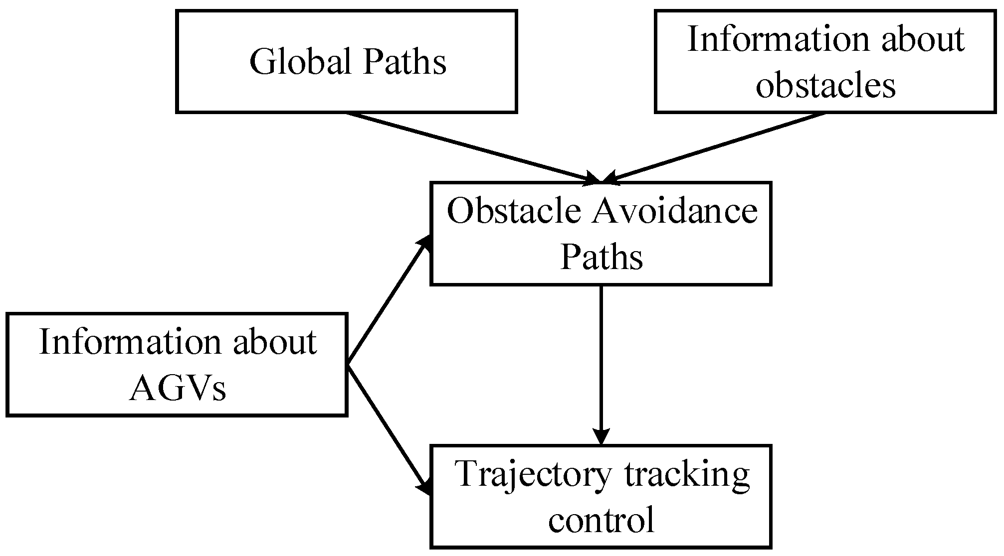
In automated container terminals, the AGV scheduling and planning problem, as well as the bottom-level control problem, are closely interrelated and interact with each other, constituting a systematic problem. In this problem, the efficient scheduling of AGVs and optimal route planning can significantly improve the operational efficiency of ports. Both levels, in turn, rely on effective bottom-level control strategies to ensure the precise traveling and safe operation of AGVs. Therefore, the three studies need to be conducted simultaneously and should consider each other’s requirements and constraints to ensure the optimality of the overall system. The occurrence of conflict and deadlock is one of the main factors affecting the operation efficiency of AGVs in ports, and most of them are caused by the long-time stagnation of AGVs due to sudden vehicle failure in ports or the change in upper layer scheduling. When a conflict or deadlock occurs at an automated container terminal, timely feedback in scheduling, planning, and control becomes crucial. If autonomous obstacle avoidance cannot be achieved, it may lead to a second round of scheduling from the upper system, significantly affecting the loading and unloading efficiency of the terminal. Therefore, AGVs must ensure timely path planning and tracking control to avoid conflict or deadlock. Safety, reliability, and high efficiency are fundamental requirements for AGVs moving goods at automated container terminals [5]. Although some studies have been conducted to address efficiency gains in transportation, they still do not meet the needs of automated terminals [6,7]. Consequently, there is an urgent need for reasonable path planning and a control strategy for AGVs during the autonomous obstacle avoidance phase at automated container terminals. Figure 1 is a schematic diagram of a layered scheme for avoiding obstacles in the face of conflicts and deadlocks for AGVs in automated terminals.

In order to prevent the occurrence of conflict and deadlock in the horizontal transport phase at an automated terminal, AGVs need to have local path-planning schemes for autonomous obstacle avoidance. A variety of local path-planning schemes for urban vehicles have been proposed. For example, the dynamic window approach (DWA) [8,9,10] is a common path-planning algorithm that has the advantage of low computational complexity. However, this method has a poor obstacle-avoidance effect on dynamic obstacles and is not forward-looking enough. Time elastic band (TEB) [11,12,13] is also a widely used method for planning obstacle avoidance paths, which is strongly forward-looking and practical for dynamic obstacle avoidance. However, planning based on TEB may fail if the parameters and weights are not set correctly or if the environment is too demanding. In addition, the artificial potential field (APF) method is also widely used for vehicle path planning due to its ease of low-level real-time control. APF plans a rational path for a vehicle by creating an attractive and repulsive potential field between the controlled vehicle and the obstacle [14,15,16]. It can be computationally compact and easily expresses the relationship between a vehicle and the obstacles. Nevertheless, for AGVs, the local path-planning scheme not only needs to plan the desired path for obstacle avoidance but also needs to satisfy the physical constraints specific to AGVs and the port environment.

In order to satisfy this condition and to solve the problem that APFs are prone to produce locally optimal solutions, Huang et al. [17] first proposed a combination controller based on an APF and model predictive control (MPC) in intelligent vehicle infrastructure cooperative systems (IVICSs). However, the APF lacks predictive feedback for the transverse distance and can only achieve the function of driving to a straight target point. It lacks tracking ability for the initial trajectory, so it cannot be directly applied to the tracking control of an AGV. In reference [18], an MPC method based on Improved Particle Swarm Optimisation (IPSO) was proposed to solve the planning and tracking problem, but it only uses kinematic models for planning and control and lacks further improvements to the path planning scheme. Liu et al. [19] proposed using a Fuzzy Logic System (FLS) to dynamically adjust the two potential fields of APF to adapt to different types of obstacles and fusion with MPC for path planning. However, the paper does not improve the ability of vehicles to return to the original trajectory when avoiding obstacles. Wang et al. [20] proposed a simultaneous planning and control scheme, combining MPC and APF to control unmanned surface vessels. However, the APF is built without considering the effect of the relative speed of dynamic obstacles.

For the control level of an AGV, it is necessary for the AGV to track the desired path accurately and quickly. There are many AGV control schemes available such as Proportional Integral Derivative (PID) control, Sliding Mode Control (SMC), Fuzzy Logic Control (FLC), etc. [21,22,23]. The tracking effect of PID is still not well-suited to high-speed and non-linear trajectories [24,25]. SMC is also a mainstream control method for mobile robots, which has the advantage of being insensitive to parameter changes and perturbations but has a chattering phenomenon [26,27,28]. FLC is robust to disturbances and parameter changes [29,30]. However, the control accuracy of this method still needs to be improved. For vehicle motion control, vehicle dynamics modelling simplifies control issues, followed by multivariate control algorithms for design and optimisation. AGV control is typically seen as a multivariate problem. Variables like speed and steering angle are interrelated and must be coordinated, making it essential to consider their interactions for effective AGV control. Considering the nonlinearity and strong coupling of the AGV control process, commonly used multivariate control algorithms such as MPC and linear quadratic regulator (LQR) have also been widely used in AGV control problems. MPC has the advantage of dealing with constraints and thus provides a stable theoretical framework for the control of AGVs [31,32]. MPC excels in multivariable control but is limited by computational cost, real-time delays, and model sensitivity. The LQR requires no real-time optimisation, has minimal computational demand, and a quick response speed. This makes it ideal for control problems requiring high system dynamic response speeds. The LQR is widely used in many practical problems [33,34] because it can be applied to a variety of systems, as well as multi-input and multi-output control problems. For AGVs, the LQR control scheme optimizes system performance and balances trajectory accuracy and energy consumption. Secondly, the LQR has excellent system stability, which ensures the stable traveling of AGVs in complex environments. Furthermore, the LQR simplifies the controller design process and improves efficiency. However, whether using MPC or the LQR, the setting of their weighting matrices will undoubtedly have an impact on the final control effect.

Our research indicates that existing path-planning and tracking control schemes fall short of AGV obstacle avoidance. There is a need to enhance AGVs’ dynamic adaptability. Additionally, the optimal cost function weights are crucial to the outcomes, with many scholars exploring weight optimisation. Qazani et al. [35] proposed an MPC-based motion cueing algorithm to calculate suitable MPC weights with fuzzy logic units and provide more efficient utilisation of the motion simulation platform. Nevertheless, its compensator unit and the application of intelligent algorithms may affect the timeliness of the response. Wang et al. [36] presented an improved PSO algorithm for adjusting the cost function of model predictive torque control, thus reducing the switching losses of the system. Yet, intelligent algorithms still lose a great deal of computational power. Elkhatem and Engin [37] suggested adjusting the weighting matrix of the LQR to compensate for the interference of the model of unmanned aerial vehicles. However, the formulae need to be established concerning the actual situation. In reference [38], the Skyhook-LQR controller was proposed, and the controller’s gain was adjusted to achieve better ride comfort. However, the proposed algorithm needs to be designed based on experimental tests.

Based on an in-depth study of the related literature, we identified a core challenge for automated terminal operations: providing immediate planning and control feedback in conflict and deadlock. Failure to effectively implement autonomous obstacle avoidance measures to ensure that AGVs travel smoothly on their intended routes may trigger secondary scheduling by higher-level systems, which will undoubtedly severely reduce loading and unloading efficiency. While this problem has been identified, we have yet to see a comprehensive solution for path planning and tracking control designed for the automated terminal environment that effectively addresses conflict and deadlock in AGVs. This research gap suggests an urgent need to develop new approaches to optimize path planning and tracking control of AGVs in ports to resolve conflict and deadlock, thereby improving loading and unloading efficiency in automated terminals. In addition, another critical challenge for ports is that it is currently difficult to establish a control scheme based on an obstacle avoidance-planning scheme that balances accuracy and real-time computational performance to match upper-level planning.

This paper mainly makes the following contributions:

• For the first time, a set of path-planning and tracking control methods for conflict and deadlock design of AGVs in automated terminals is proposed. Autonomous obstacle avoidance in the planning and control layer of automated terminal environments is a practical problem that needs to be solved, and it is also an important academic problem in the field of management and control. Although scholars have studied AGV path planning and trajectory tracking, there is not yet an autonomous obstacle avoidance method for AGVs that matches the automated terminal.
• The innovative integration of MPC, APF, and FLS theories realizes the practical function of autonomous obstacle avoidance for AGVs in automated terminals. Initially, APF establishes the numerical expression of the real-time state of obstacle vehicles and is incorporated into the MPC cost function to provide basic path planning capability for AGV autonomous obstacle avoidance. Subsequently, by inputting the real-time state of the controlled AGV into the FLS and outputting the corresponding MPC weights in real-time, we enhanced the stability of the AGV during autonomous obstacle avoidance and its ability to return to its initial trajectory. Based on these, a hybrid artificial potential field-fuzzy model prediction controller (HAPF-FMPC) was developed. Moreover, during the tracking control phase, we also use an FLS to improve real-time adaptability to different obstacle avoidance paths. This approach of integrating MPC, APF, and FLS, considering the actual working conditions of AGV autonomous obstacle avoidance, constitutes a significant application innovation entailing substantial implementation difficulties and technical challenges.
• To satisfy the requirements of accuracy and real-time performance and to emulate the actual operating conditions of AGVs in ports more closely, we rectify the planning layer’s shortcomings in the accuracy of the AGV model. We establish fuzzy LQR (FLQR) and AGV dynamics models for the lateral control of AGVs and construct a longitudinal controller to match the speed planning of AGVs.

2. Programme Framework and Modelling

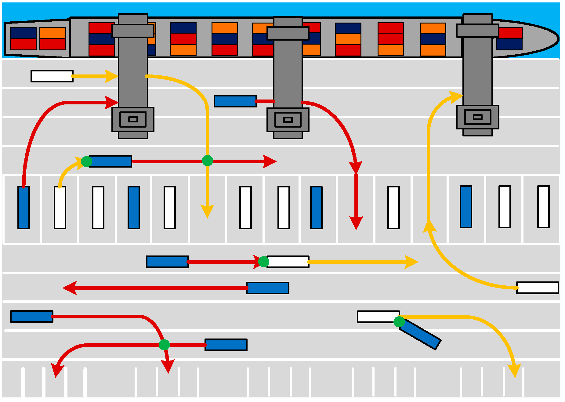
Figure 2 shows that AGVs in automated terminals follow pre-set routes to load/unload points but can also face conflicts and deadlocks at intersections and during task assignments. Post-task, AGVs are repositioned based on new schedules. While planning ensures efficiency and safety, resolving conflicts and deadlocks is vital.

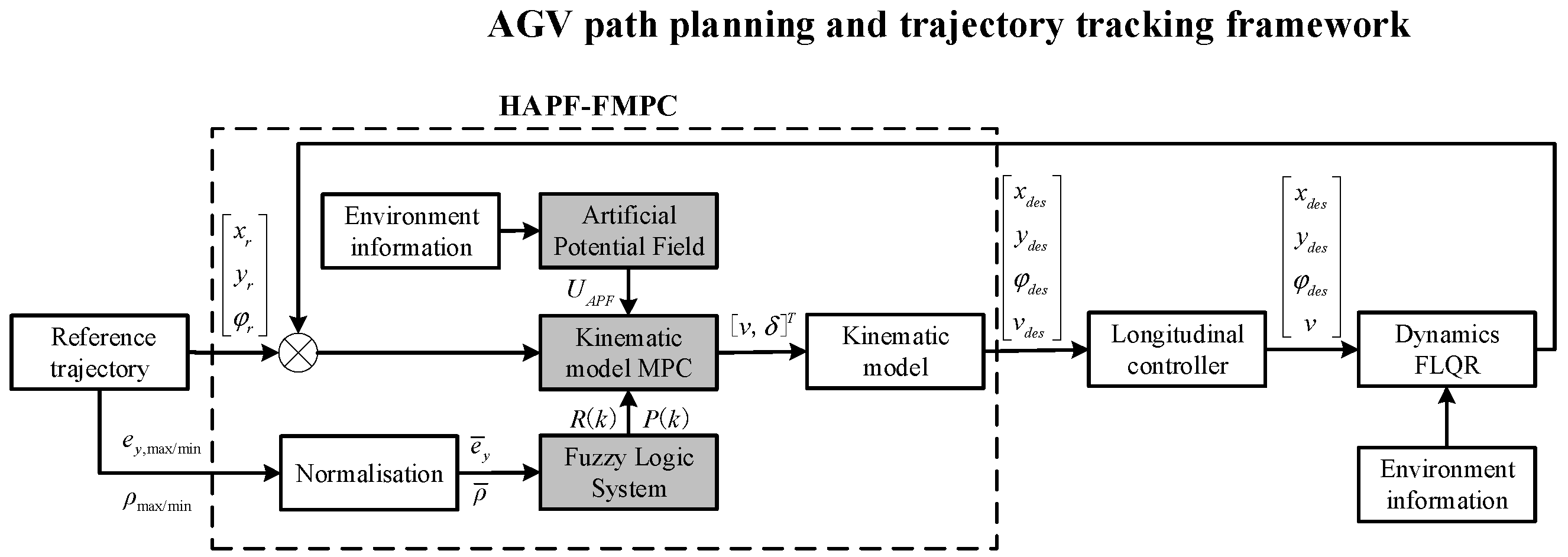
In this paper, a HAPF-FMPC path planner based on the kinematic model of an AGV was built using the AGV and related exchange information obtained in IVICSs. Then, the transverse FLQR path tracker was built based on the AGV dynamics model, and then, the longitudinal PI controller was built. Finally, the path planning and trajectory tracking of AGVs in the presence of obstacles were realised. The structure of the scheme is shown in Figure 3.

To ensure rapid AGV planning, this paper utilises the AGV kinematic model for path planning and establishes the AGV dynamics model for trajectory tracking. The kinematic model views AGV motion geometrically, while the dynamics model offers a detailed mathematical representation for more realistic control.

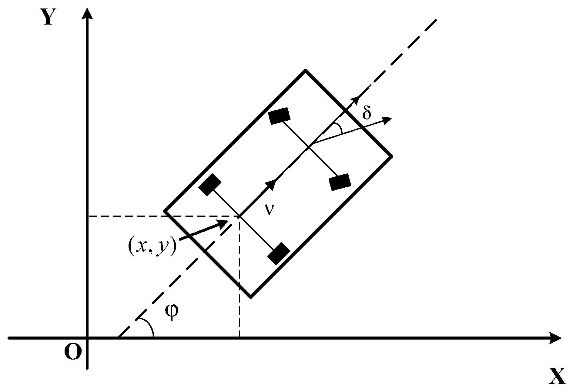
Firstly, a mathematical model of an AGV is established to describe an AGV’s movement. The kinematic model of the AGV is shown in Figure 4 [39].

As shown in Figure 4, with XOY as the geodetic coordinate system, the mathematical expressions in this reference coordinate can be given as follows.

$$\left[\begin{array}{c}\dot{x}\\ \dot{y}\\ \dot{\phi }\end{array}\right]=\left[\begin{array}{c}v\cos \phi \\ v\sin \phi \\ \frac{v\tan \delta }{l}\end{array}\right]$$

(1)

The state vector of the model is represented as $\chi ={[x,y,\phi ]}^T$, where $x$ and $y$ stand for the cartesian coordinates of the position of the AGV, and $\phi$ denotes the counter clockwise orientation of the AGV from the x-axis. $u={[v,\delta ]}^T$ denotes the AGV’s control input vector, where $v$ denotes the speed of the controlled AGV and $\delta$ denotes the front wheel steering angle of the controlled AGV. $l$ is the wheelbase. For the reference path, the path can be described in terms of the motion of the controlled AGV.

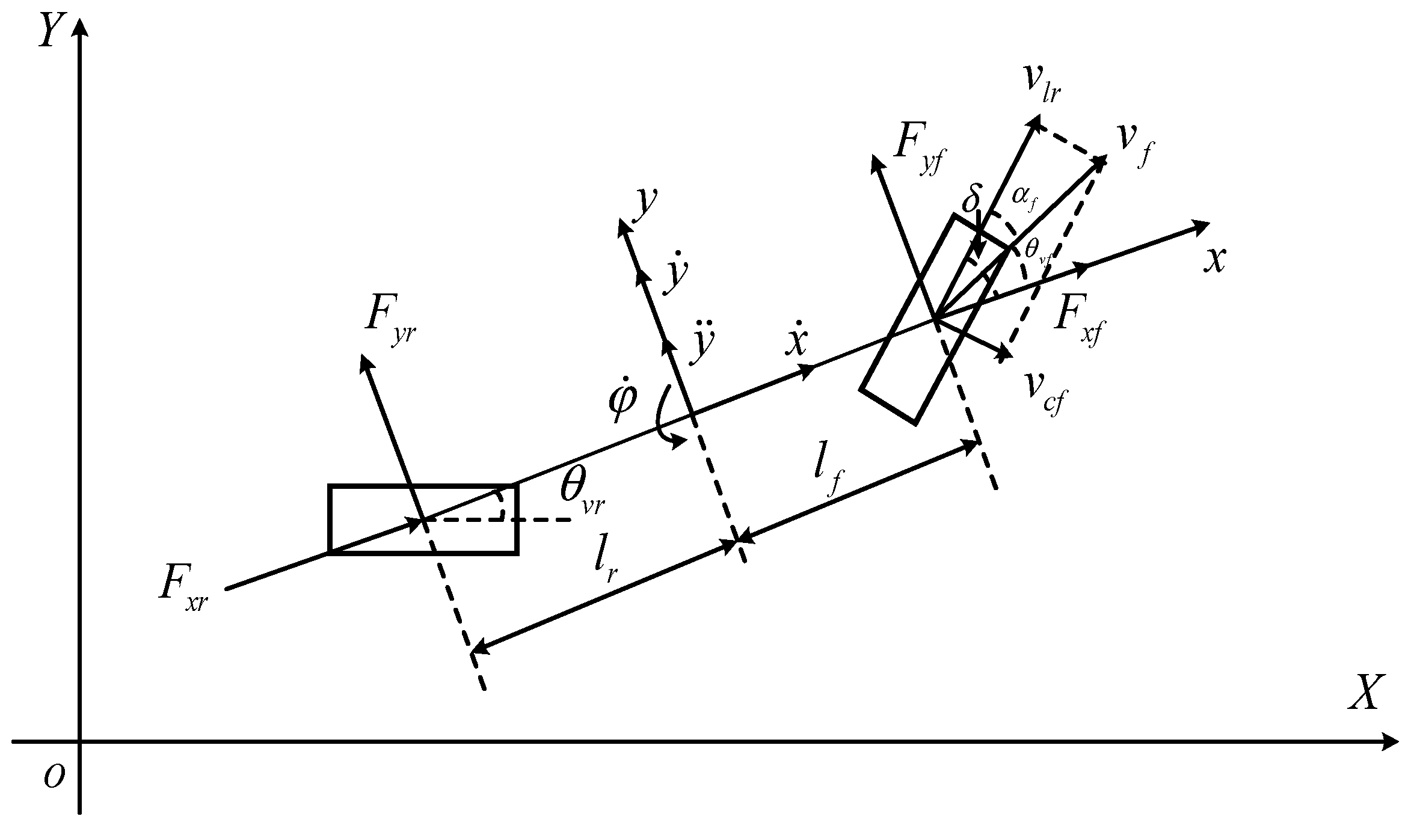
The kinematic model of the vehicle is used in HAPF-FMPC for vehicle path planning. Then, the dynamics of the AGV are modelled for use in tracking the resulting desired trajectory. During this tracking, the created AGV model closely resembles the real vehicle, ensuring a control effect that mirrors actual conditions. Thus, we propose the following dynamic model of AGV as in Figure 5 [39].

According to Newton’s second law, it can be concluded that:

$$m{a}_y=F_{yf}+F_{yr},$$

(2)

where $a_y$ is the lateral acceleration at the centre of mass of the vehicle. $F_{yf}$ and $F_{yr}$ represent the ground forces on the front wheels and rear wheels. The equation for lateral acceleration can be obtained as follows:

$$a_y=\ddot{y}+v_x\dot{\phi },$$

(3)

$$m\left(\ddot{y}+v_x\dot{\phi }\right)=F_{yf}+F_{yr},$$

(4)

where $\ddot{y}$ is the acceleration resulting from lateral movement of the vehicle along the y-axis of the body degree and $v_x\dot{\phi }$ is the centripetal acceleration resulting from the transverse pendulum motion of the body. The equation for the torque balance of the vehicle around the z-axis is:

$$I_z\ddot{\phi }=F_{yf}{l}_f-F_{yr}{l}_r,$$

(5)

where $l_f$ is the distance from the centre of mass to the front axle and $l_r$ is the distance from the centre of mass to the rear axle. Based on the assumption of a small lateral deflection angle, the lateral tyre forces on the front and rear wheels of the AGV can be obtained as:

$$F_{yf}=2C_{\alpha f}\left(\delta -{\theta }_{vf}\right),$$

(6)

$$F_{yr}=-2C_{\alpha r}{\theta }_{vr},$$

(7)

where $C_{\alpha f}$ is the front wheel cornering stiffness, $C_{\alpha r}$ is the rear wheel cornering stiffness, and $m$ is the mass of the AGV. Taking the transverse position $y$, transverse position change rate $\dot{y}$, transverse pendulum angle $\phi$, and transverse pendulum angle change rate $\dot{\phi }$ as state quantities, the rewritten state equations are as follows. Finally, the vehicle dynamics model can be obtained as:

$$\frac{d}{dt}\left[\begin{array}{c}y\\ \dot{y}\\ \phi \\ \dot{\phi }\end{array}\right]=\left[\begin{array}{cccc}0& 1& 0& 0\\ 0& -\frac{2C_{\alpha f}+2C_{\alpha r}}{m{v}_x}& 0& -v_x-\frac{2l_f{C}_{\alpha f}-2l_r{C}_{\alpha r}}{m{v}_x}\\ 0& 0& 0& 1\\ 0& \frac{2C_{\alpha r}{l}_r-2C_{\alpha f}{l}_f}{I_z{v}_x}& 0& -\frac{2l_f^2{C}_{\alpha f}+2l_r^2{C}_{\alpha r}}{I_z{v}_x}\end{array}\right]\left[\begin{array}{c}y\\ \dot{y}\\ \phi \\ \dot{\phi }\end{array}\right]+\left[\begin{array}{c}0\\ \frac{2C_{\alpha f}}{m}\\ 0\\ \frac{2l_f{C}_{\alpha f}}{I_z}\end{array}\right]\delta$$

(8)

3. APF Establishment and Speed Planning

During AGV operation, factors like surrounding AGVs, road conditions, the current position, and velocity influence its decisions. To ensure precise obstacle avoidance with the IVICS, this information is depicted using APF modelling. However, APF is not always viable for obstacle avoidance. If the IVICS data suggests avoidance is impractical, conflicts between AGVs can be mitigated with speed planning.

3.1. APF Modelling for Environment Interaction

The APF’s value for each point to be created will represent the risk level of the current AGV’s location. The lower the APF value of the AGV, the lower the risk of the current position. Based on the APF, the following potential fields are established:

$$U_{APF}=U_{obs}+U_{lane}+U_v,$$

(9)

where $U_{obs}$ represents the surrounding obstacle’s potential field; $U_{lane}$ represents the lane line potential field; $U_v$ represents the velocity potential field between the controlled AGV and the obstacle vehicle; and $U_{APF}$ represents the total APF value of the current AGV’s location. The APF will dynamically adjust to changes in the environment. The detailed model for determining the identified obstacle avoidance is as follows.

3.1.1. Surrounding Obstacle’s Potential Field

The surrounding obstacle’s potential field is created to gauge its impact on the AGV, ensuring it maintains a safe distance. Since the AGV perceives varying danger levels in vertical and horizontal directions near obstacles, the function is used to model the potential field of the obstacle vehicle. Based on reference [40], we can determine that when $d>d_0$, the surrounding obstacle’s potential field can be defined as follows:

$$U_{obs}=\frac{1}{2}{k}_{rep}{\left(\frac{1}{d}-\frac{1}{d_0}\right)}^2,$$

(10)

where $k_{rep}$ is the repulsive gain coefficient; $d$ is the distance between the AGV and the obstacle; and $d_0$ is the distance that the obstacle can influence.

3.1.2. Lane Line Potential Field

While the AGV is in motion, lane restrictions are vital to ensure its obstacle avoidance stays within lane lines, thus preventing disruptions to other vehicles. Based on reference [17], the relationship of the lane line constraint can be expressed by the lane line potential field, which is defined as follows:

$$u_{lane}=A_{lane}\exp \left(-\frac{d_{\mathrm{lane},i}}{2{\sigma }_l^2}\right),$$

(11)

where $A_{lane}$ represents the gain coefficient of the road potential field; $d_{\mathrm{lane},i}$ is the distance between the AGV and the lane line; and ${\sigma }_l$ is the convergence coefficient of the road potential field. The overall potential field of lane lines is as follows:

$$U_{\mathrm{lane} }={\displaystyle \sum _i{u}_{\mathrm{lane} }}(i).$$

(12)

As shown in Figure 2, the port differs from city roads in obstacle avoidance during turns. AGVs in ports do not use lane line potential fields at turning points. However, this affects the parameters of velocity and obstacle potential fields in various environments.

3.1.3. AGV Velocity Potential Field

In addition to obstacle distance and lane line effects, the speeds of both the obstacle and the controlled AGV are crucial. Considering their speed interaction enhances AGV safety. From reference [19], for adapting to the speed of the AGV and the dynamic environment around it, the velocity potential field model can be established as follows:

$$U_v=k_v\left(v-v_{obs}\right),$$

(13)

where $k_v$ is the gain coefficient of the velocity potential field; $v$ is the current speed of the controlled AGV; and $v_{obs}$ is the velocity of the dynamic obstacle.

3.2. Speed Planning for AGV

By comparing the judgments, we can determine whether the AGV can avoid obstacles at this time. This study evaluates whether AGVs can safely avoid obstacles by comparing the predicted positions of obstacles with the positions of AGVs after circumventing obstacles across the width of two lanes. The approach involves predicting whether AGVs maintain an adequate safety distance after avoidance manoeuvres, thus providing a preliminary assessment of their obstacle avoidance safety. If the AGV is unable to avoid obstacles, the APF is not used for obstacle avoidance. Speed planning is carried out based on the initial trajectory.

$$x_{obs}^{\prime }=x_{obs}+\frac{x_{obs}-x_c+d_0}{\left(v_{des}-v_{obs}\right)}{v}_{obs},$$

(14)

$$x_{pre}=x_c+\frac{2d_0+2l_0+(x_{obs}^{\prime }-x_{obs})}{\left(v_{des}-v_{obs}\right)}{v}_{des}$$

(15)

where $x_{obs}$ and $x_c$ are the current obstacle position and the current position of the AGV, which are obtained with the IVICS; $l_0$ represents the distance between the centrelines of lanes; and $x_{pre}$ represents the predicted position of the controlled AGV after the end of the lane change obstacle-avoidance process. If there are loading and low-speed zones or other non-obstacle avoidable objects within $x_{pre}$, the controlled AGV decelerates to follow the low-speed obstacles. An expected speed planning model is created, as shown in the following.

$$v_{des}=\{\begin{array}{cc}{v}_{obs}& \mathrm{Slow} \mathrm{to} \mathrm{follow} \\ 0& \mathrm{Brake} \\ v^{\prime }& \mathrm{Other} \mathrm{situations}\end{array}$$

(16)

where $v^{\prime }$ is the original desired speed; $v_{des}$ is the current desired speed; and $v_{obs}$ is the speed of the low-speed obstacle. In velocity planning, the AGV accelerates and decelerates to reach the target velocity. For the AGV to have enough distance to decelerate to the same speed as the low-speed obstacle, we set the distance at the beginning of deceleration as $h$. $h$ is calculated with the following equation

$$t_h=\frac{v-v_{obs}}{a},$$

(17)

$$h=d_0+v{t}_h-\frac{1}{2}a{t}_h^2$$

(18)

4. HAPF-FMPC Design

In this paper, we propose a path-planning scheme HAPF-FMPC for AGVs. The established APF is combined with the MPC cost function and FLS is established to dynamically adjust the weight coefficients of the cost function to form HAPF-FMPC.

4.1. Establishing the Cost Function of HAPF-FMPC

For controlled AGV obstacle avoidance path planning, the cost function needs to reflect the tracking performance of the desired path and speed, as well as the weighted combination of the constructed APF values and control increments.

In traditional MPC, the cost function is as follows when no APF is added:

$$\begin{array}{ll}\min J\left(k_1\right)& ={\displaystyle \sum _{i=1}^{N_c}\Vert \Delta u(}k+i-1|k){\Vert }_{R(k)}^2+\rho {\epsilon }^2\\ & \hspace{1em}+{\displaystyle \sum _{i=1}^{N_p}{\Vert \eta (k+i|k)-{\eta }_{\mathrm{ref}}(k+i|k)\Vert }_{P(k)}^2}\end{array}$$

(19)

Then, when the APF is added the cost function is:

$$\begin{array}{ll}\min J(k)& ={\displaystyle \sum _{i=1}^{N_p}{\Vert U_{\mathrm{obs} }(k+i|k)\Vert }_Q^2}+{\displaystyle \sum _{i=1}^{N_p}{\Vert U_{\mathrm{lane} }(k+i|k)\Vert }_Q^2}\\ & \hspace{1em}+{\displaystyle \sum _{i=1}^{N_c}{\Vert U_v(k+i-1|k)\Vert }_Q^2}+J\left(k_1\right)\end{array},$$

(20)

where $Q$, $R(k)$, and $P(k)$ are the corresponding weight coefficients, and $R(k)$ and $P(k)$ are the dynamically adjusted weights; $N_p$ represents prediction horizon; $N_c$ represents the control horizon; ${\eta }_{\mathrm{ref} }(k+i|k)$ represents the expected state given; $\epsilon$ is the relaxation factor; and $\rho$ is the corresponding weight of the relaxation factor. $k$ represents the current moment when obstacle avoidance is required: $k_1$ = $k$. The cost function mainly includes three parts:

${\displaystyle \sum _{i=1}^{N_p}{\Vert U_{obs}(k+i|k)\Vert }_Q^2}+{\displaystyle \sum _{i=1}^{N_p}{\Vert U_{lane}(k+i|k)\Vert }_Q^2}+{\displaystyle \sum _{i=1}^{N_c}{\Vert U_v(k+i-1|k)\Vert }_Q^2}$ represents the value of the APF. When the controlled AGV avoids obstacles, it finds the points with the minimum APF value established under the reference path as the optimal path.

${\displaystyle \sum _{i=1}^{N_c}\Vert \Delta u(}k+i-1|k){\Vert }_{R(k)}^2$ represents the change degree of control increments. Introducing this item aims to prevent significant changes in the control quantity. The control increment changes smoothly to avoid a significant change in the AGV’s motion state and improve safety.

${\displaystyle \sum _{i=1}^{N_P}{\Vert \eta (k+i|k)-{\eta }_{\mathrm{ref}}(k+i|k)\Vert }_{P(k)}^2}$ represents the tracking effect of the AGV on the global path given by the upper layer and the maintaining effect of the desired speed. The smaller the error, the better the tracking and maintaining effect of the controlled AGV on the global path.

Given the AGV’s dynamics and driving conditions, path planning and tracking should match real operating traits. Control volume constraints affect longitudinal speed and the front wheel angle, while control increment constraints relate to control volume changes over sampling time.

The specific constraints are as follows [39]:

$$\Delta u_{\min }\le \Delta u\le \Delta u_{\max },$$

(21)

$$u_{\min }\le A\Delta u+u_t\le u_{\max }.$$

(22)

$u_t$ is the Kronecker product of the column vector with $N_c$ rows and the actual control volume at the previous moment in time. And $A=\left[\begin{array}{ccccc}{I}_2& 0& 0& \cdots & 0\\ I_2& I_2& 0& \cdots & 0\\ I_2& I_2& I_2& \cdots & 0\\ \cdots & \cdots & \cdots & \ddots & 0\\ I_2& I_2& I_2& \cdots & I_2\end{array}\right]$, $A$ with row $N_c$ and column $N_c$.

4.2. Design of the FLS

In order to improve the stability of the AGV path and the ability to return quickly to the initially planned path, an improved HAPF-MPC based on FLS is proposed. The control scheme can adaptively adjust the weighting factors of the cost function according to the heading error and the lateral error.

FLS is used to optimise the weighting coefficients of the MPC cost function online. This paper sets $Q$ to a fixed value. At the same time, the optimal combination of weight coefficients is obtained by adjusting $P$ and $R$. According to the reference [41], we adjust the weights of HAPF-FPMC based on the fuzzy adjustment method proposed by them. Firstly, the transverse deviation and the difference between the front-wheel angle and expectation are normalised:

$${\overline{e}}_y=\frac{e_{y,\max }-\left|e_y\right|}{e_{y,\max }-e_{y,\min }},$$

(23)

$$\overline{\rho }=\frac{{\rho }_{\max }-\rho }{{\rho }_{\max }-{\rho }_{\min }},$$

(24)

where $e_y$ represents current lateral error; $e_{y,\max }$ and $e_{y,\min }$ represent the maximum and minimum lateral error in the tracking state, respectively; $\rho$ is the difference between the current front-wheel turning angle and the desired front-wheel turning angle at the next moment; ${\rho }_{\max }$ is the maximum difference between the front-wheel rotation angle and the next moment of the front-wheel rotation angle; and ${\rho }_{\min }$ is the minimum difference between the front-wheel rotation angle and the next moment of the front-wheel rotation angle. We set $e_{y,\max }$ to 5, $e_{y,\min }$ to 0, ${\rho }_{\max }$ to 0.54, and ${\rho }_{\min }$ to 0.

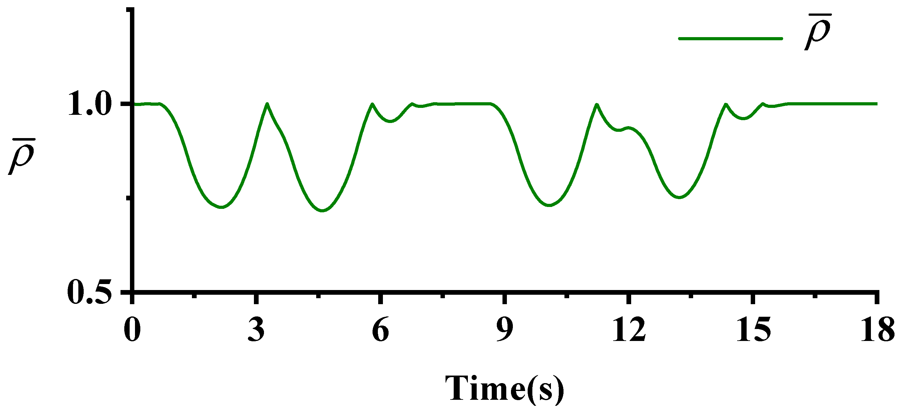
Given the normalised error values for the front-wheel angle and lateral distance and a fuzzy subset of 5, the input is {0,0.25,0.5,0.75,1}, with fuzzy control subsets as {NB (negative big), NS (negative small), ZO (zero), PS (positive small), PB (positive big)}. The Gaussian membership function is chosen. The output variables range from [0, 1], serving as weight adjusters. Their fuzzy control subset is similar to the input, using the Gaussian function. Specific rules as in

Table 1. Control rules $\Delta P(k)$.

$\mathbf{\Delta }\mathit{P}$		${\overline{\mathit{e}}}_{\mathit{y}}$
		NB	NS	ZO	PS	PB
$\overline{\rho }$	NB	PB	PB	PS	ZO	NS
	NS	PB	PS	ZO	NS	NB
	ZO	PS	ZO	ZO	NS	NB
	PS	ZO	ZO	NS	NB	NB
	PB	ZO	NS	NB	NB	NB

.

The rule-making principle of the FLS is designed to ensure that the AGV can improve the control performance of the HAPF-FMPC. At the same time, it helps the AGV to return quickly to the reference path after obstacle avoidance is complete. When the lateral deviation is large, more emphasis should be placed on the goal that the AGV is tracking, which can quickly bring the AGV back to the reference path, so the corresponding weight of $P$ should be increased. When $R$ is increased, it ensures that the AGV is more stable with a small tracking error. $\Delta P$ and $\Delta R$ are the corresponding regulatory factors. Based on the above analysis, the design control rules of $\Delta P$ are as follows, $\Delta R=1-\Delta P$:

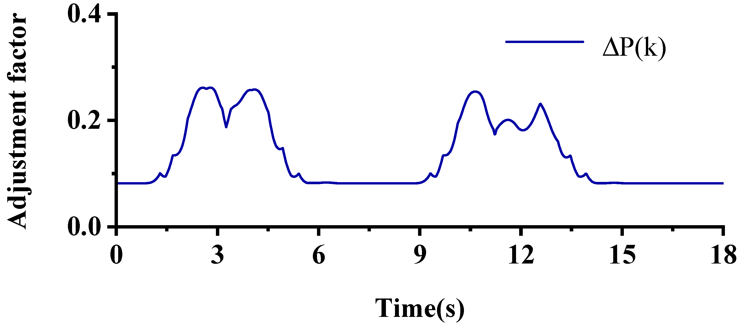
The outputs of the FLS are not directly used as the weighting coefficients for the HAPF-FMPC in order to improve adaptability to different environments. They are used as a correction for the weight coefficient to adjust the weight coefficient, where the adjustment formulas for $P(k)$ and $R(k)$ are:

$$P(k)=P_0{10}^{\Delta P(k)},$$

(25)

$$R(k)=R_0{5}^{\Delta R(k)},$$

(26)

where $P(k)$ and $R(k)$ are the final output weight coefficients of HAPF-FMPC; and $P_0$ and $R_0$ are the initial weight coefficients of HAPF-FMPC.

5. Tracking Controller Design

Because MPC uses a large amount of computation in the path planning phase, the requirements for computing power are large. To suit the engineering requirements, the LQR is used for trajectory tracking to improve the tracking control’s real-time nature. In addition, the FLS is established to dynamically adjust the weights of the LQR once before each obstacle avoidance to suit the tracking of the AGV’s obstacle avoidance path. In addition to this, the speed of the AGV is tracked using a PI controller.

Based on the vehicle dynamics model, the vehicle body error model is established. The following state errors are obtained from the desired state:

$$e_2=\phi -{\phi }_{\mathrm{des}},$$

(27)

$${\dot{e}}_2=\dot{\phi }-{\dot{\phi }}_{\mathrm{des} },$$

(28)

$$\begin{array}{ll}{\ddot{e}}_1=& -\frac{2C_{\partial r}+2C_{\partial f}}{m{v}_x}{\dot{e}}_1+\frac{2C_{\partial r}+2C_{\partial f}}{m}{e}_2+\left(\frac{2C_{\partial r}{l}_r-2C_{\partial f}{l}_f}{m{v}_x}-v_x\right){\dot{e}}_2\\ & +\frac{2C_{\partial r}{l}_r-2C_{\partial f}{l}_f}{m{v}_x}{\dot{\phi }}_{\mathrm{des}}+\frac{2C_{\partial f}\delta }{m}\end{array},$$

(29)

$$\begin{array}{ll}{\ddot{e}}_2=& \frac{2C_{\partial r}{l}_r-2C_{\partial f}{l}_f}{I_z{v}_x}{\dot{e}}_1+\frac{2C_{\partial f}{l}_f-2C_{\partial r}{l}_r}{I_z}{e}_2-\frac{2C_{\partial f}{l}_f{}^2+2C_{\partial r}{l}_r{}^2}{I_z{v}_x}{\dot{e}}_2\\ & -\frac{2C_{\partial r}{l}_r{}^2+2C_{\partial f}{l}_f{}^2}{I_z{v}_x}{\dot{\phi }}_{\mathrm{des}}+\frac{2C_{\partial f}{l}_f}{I_z}\delta \end{array}.$$

(30)

The error state equation can be obtained after the above equation:

$$\begin{array}{ll}\frac{d}{dt}\left[\begin{array}{c}{e}_1\\ {\dot{e}}_1\\ e_2\\ {\dot{e}}_2\end{array}\right]& =\left[\begin{array}{cccc}0& 1& 0& 0\\ 0& -\frac{2C_{\partial r}+2C_{\partial f}}{m{v}_x}& \frac{2C_{\partial r}+2C_{\partial f}}{m}& \frac{2C_{\partial r}{l}_r-2C_{\partial f}{l}_f}{m{v}_x}\\ 0& 0& 0& 1\\ 0& \frac{2C_{\partial r}{l}_r-2l_f{C}_{\partial f}}{I_z{v}_x}& \frac{2C_{\partial f}{l}_f-2l_r{C}_{\partial r}}{I_z}& -\frac{2C_{\partial f}{l}_f^2+2C_{\partial r}{l}_r^2}{I_z{v}_x}\end{array}\right]\left[\begin{array}{c}{e}_1\\ {\dot{e}}_1\\ e_2\\ {\dot{e}}_2\end{array}\right]\\ & +\left[\begin{array}{c}0\\ \frac{2C_{\partial f}}{m}\\ 0\\ \frac{2l_f{C}_{\partial f}}{I_z}\end{array}\right]\delta +\left[\begin{array}{c}\frac{2C_{\partial r}{l}_r-2C_{\partial f}{l}_f}{m{v}_x}-v_x\\ 0\\ {\phi }_{\mathrm{des} }\\ -\frac{2C_{\partial r}{l}_r^2+2C_{\partial f}{l}_f^2}{I_z{v}_x}\end{array}\right]{\dot{\phi }}_{\mathrm{des} }\end{array}$$

(31)

The simplification of the above equation can be obtained as:

$$\dot{x}=AX+Bu.$$

(32)

In order to be consistent with the HAPF-FMPC trajectory planning time step, the established state space was discretised. The control problem is transformed into a minimum value problem for solving the performance function using a state–space equation.

$$\min J(k)={\displaystyle \sum _{i=1}^{+\infty }\left[x^T(k)Qx(k)+u^T(k)Ru(k)\right]}.$$

(33)

Based on the optimal sequence of control obtained with iteration, the control quantity of the LQR controller of the AGV is obtained as follows [42]:

$$u=-\left[{\left(R+B^{T}PB\right)}^{-1}{B}^{T}PA\right]X=-KX.$$

(34)

During AGV obstacle avoidance, varying obstacle speeds result in different path planning. A higher relative speed between the AGV and the obstacle increases the avoidance distance and AGV tracking performance needs. To accommodate this, the LQR weighting factors are adjusted before each avoidance after normalising the current distance error and AGV’s relative velocity.

$${\overline{e}}_{yc}=\frac{e_{y,\max }-\left|e_{yc}\right|}{e_{y,\max }-e_{y,\min }},$$

(35)

$${\overline{v}}_a=\frac{v_a{}_{\max }-v_a}{v_a{}_{\max }-v_a{}_{\min }},$$

(36)

where ${\overline{e}}_{yc}$ is the current distance error of the AGV; $v_a$ is the relative speed between the desired speed of the controlled AGV and the dynamic obstacle; and $v_a{}_{\max }$ and $v_a{}_{\min }$ are the values of the maximum and minimum relative speeds. We set $e_{y,\max }$ to 0.2, $e_{y,\max }$ to 0, $v_a{}_{\max }$ to 5, and $v_a{}_{\min }$ to 0.

The FLS adjusts the LQR weighting factors based on the current distance error and the AGV’s relative speed to the obstacle. The weighting factors of the next LQR are judged by the two factors. When the current distance error and the degree of future trajectory offset are large, $Q$ is increased to ensure the path-tracking ability of the AGV and, vice versa, $R$ is increased appropriately to improve the tracking control performance.

For the FLS settings, both the input and output are set to Gaussian functions. The input is normalised to have an input range of [0, 1], and the output range is [10, 100]. Similarly, we express them as {NB, NS, ZO, PS, PB}. Using the FLS, the $Q_l$ weight value of the LQR path tracker during obstacle avoidance is the output, then $R_l=100-Q_l$. Specific rules as in

Table 2. Control rules $Q_l$.

${\mathit{Q}}_{\mathit{l}}$		${\overline{\mathit{v}}}_{\mathit{a}}$
		NB	NS	ZO	PS	PB
${\overline{e}}_{yc}$	NB	PB	PB	PB	PS	PS
	NS	PB	PB	PS	PS	ZO
	ZO	PB	PS	PS	ZO	NB
	PS	PS	PS	ZO	NS	NB
	PB	PS	ZO	NS	NB	NB

.

6. Simulation Results

This study uses adaptive schemes tested using simulations in MATLAB/Simulink. The simulation scenarios were established specifically to highlight the effectiveness of our proposed scheme. Further, the superiority of the proposed scheme over alternative approaches was illustrated with a comparative analysis. Pertinent parameters were set as follows: a tolerance of 6 × 10⁻² was set in MATLAB/Simulink for solving the optimisation problem (see

Table 3. APF basic parameters.

Symbol	Parameters	Value
$d_0$	safe distance of APF	7 m
$k_{\mathrm{rep} }$	repulsive potential field gain coefficient	20
$k_v$	velocity potential field gain coefficient	30
$k_{\mathrm{repc} }$	repulsive potential field gain coefficient (corner)	20
$k_{vc}$	velocity potential field gain coefficient (corner)	30
$A_{\mathrm{lane} }$	road potential field coefficient	2.7
${\sigma }_l$	convergence coefficient of lane lines potential field	1

,

Table 4. AGV basic parameters.

Symbol	Parameters	Value
$l$	AGV’s wheelbase	2.9 m
$C_{\partial f}$	front wheel cornering stiffness	66,900
$C_{\partial r}$	rear wheel cornering stiffness	62,700
$l_f$	distance from the centre of mass to the front axle	1.232 m
$l_r$	distance from the centre of mass to the rear axle	1.468 m
$l_z$	rotational inertia around the z-axis	4175 kg·m2
$m$	mass of the AGV	1723 kg

and

Table 5. MPC and LQR basic parameters.

Symbol	Parameters	Value
$N_p$	predictive horizon	100
$N_c$	control horizon	50
$Q_0$	weighting factor for MPC	2550
$R_0$	weighting factor for MPC	990
$\rho$	relaxation factor weights	50
$P$	controller weighting coefficient	6
$T$	sampling time	0.02 s
$a$	acceleration of AGV	1 m/s2
$u_{\min }$	minimum control error	[−0.1, −0.54] rad
$u_{\max }$	maximum control error	[0.1, 0.332] m/s
$\Delta u_{\min }$	minimum control increments	[−0.02; −0.00328]
$\Delta u_{\max }$	maximum control increments	[0.02; 0.00328]
$Q_l$	initial weighting factor for LQR	10
$R_l$	initial weighting factor for LQR	10

).

6.1. HAPF-FMPC

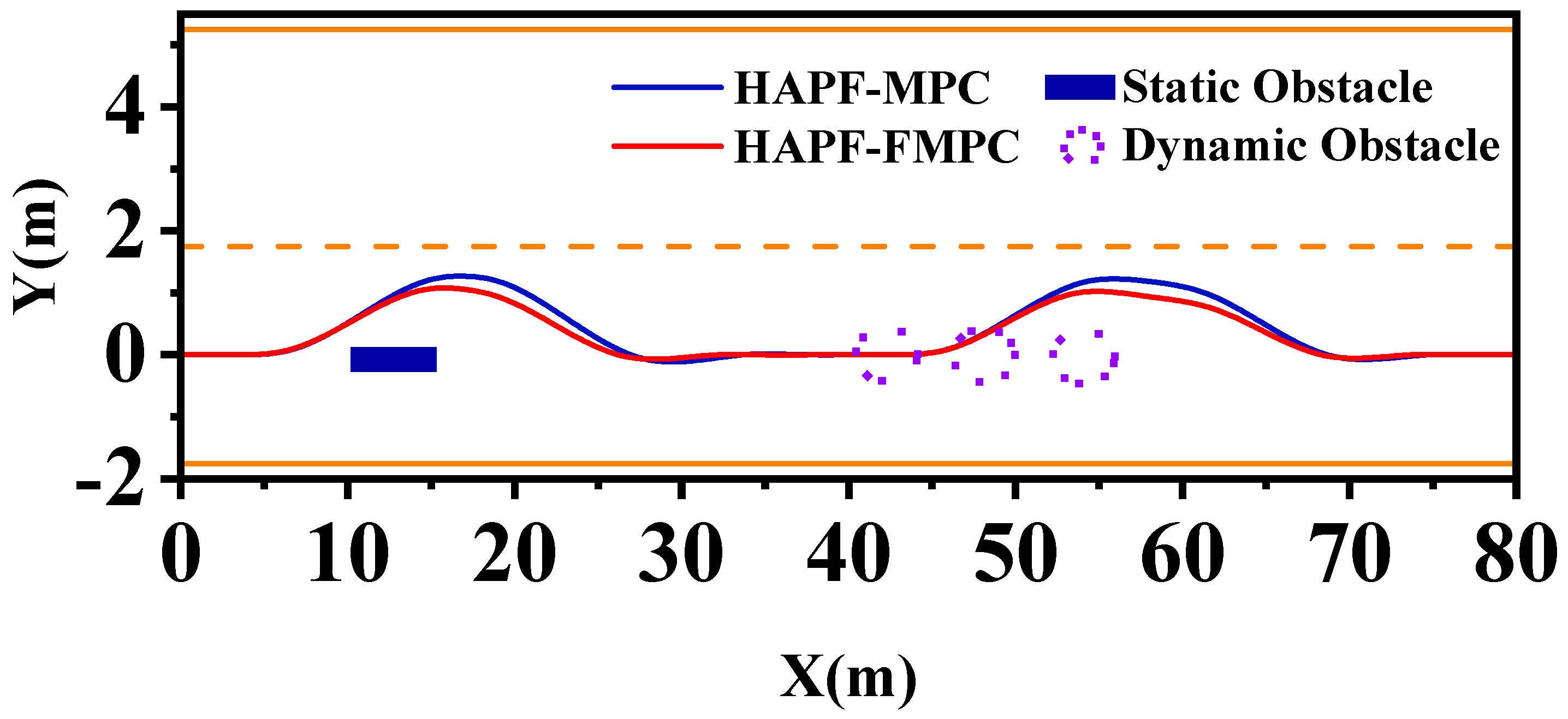
This study illustrates the efficacy of the HAPF-FMPC path planner in the context of static and dynamic obstacle avoidance. The AGV operates on a two-lane road with each lane spanning a width of 3.5 m. In this case, a static obstacle is located at x = 10 m, and a dynamic obstacle is moving forward at x = 45 m with a speed of 0.5 m/s. During the simulation strictly dedicated to the HAPF-FMPC, the parameter $\rho$ is maintained at 100.

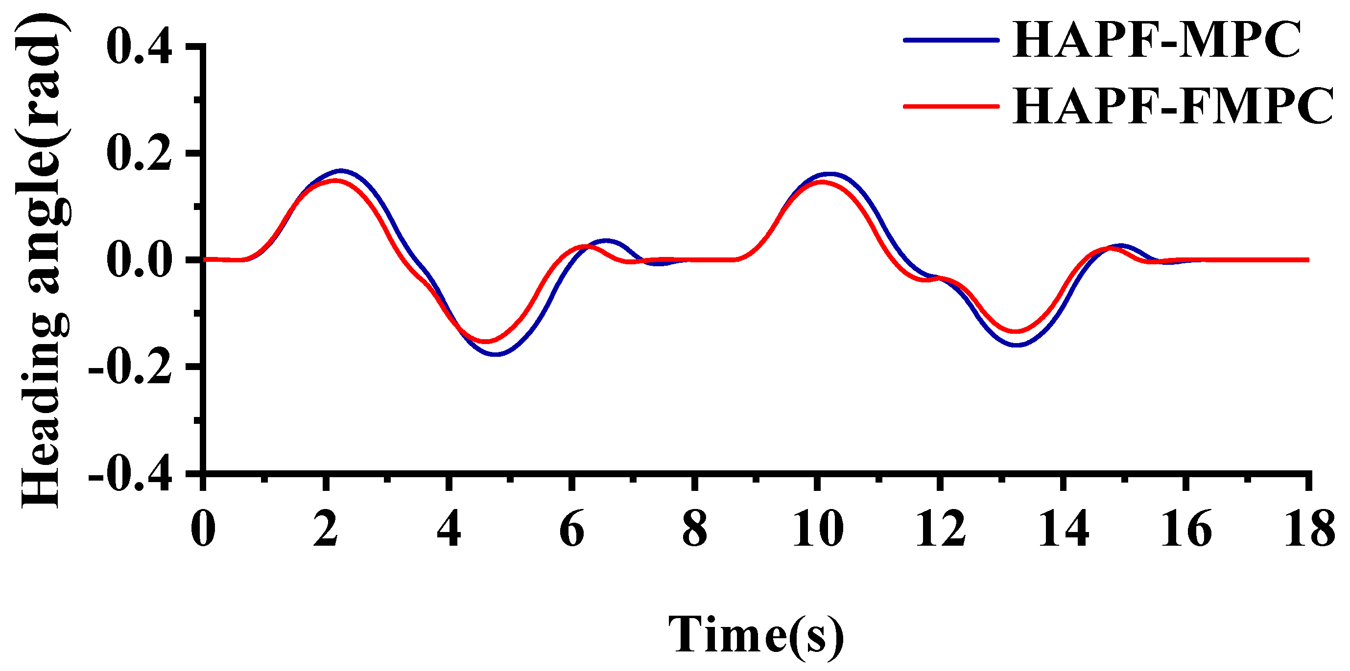
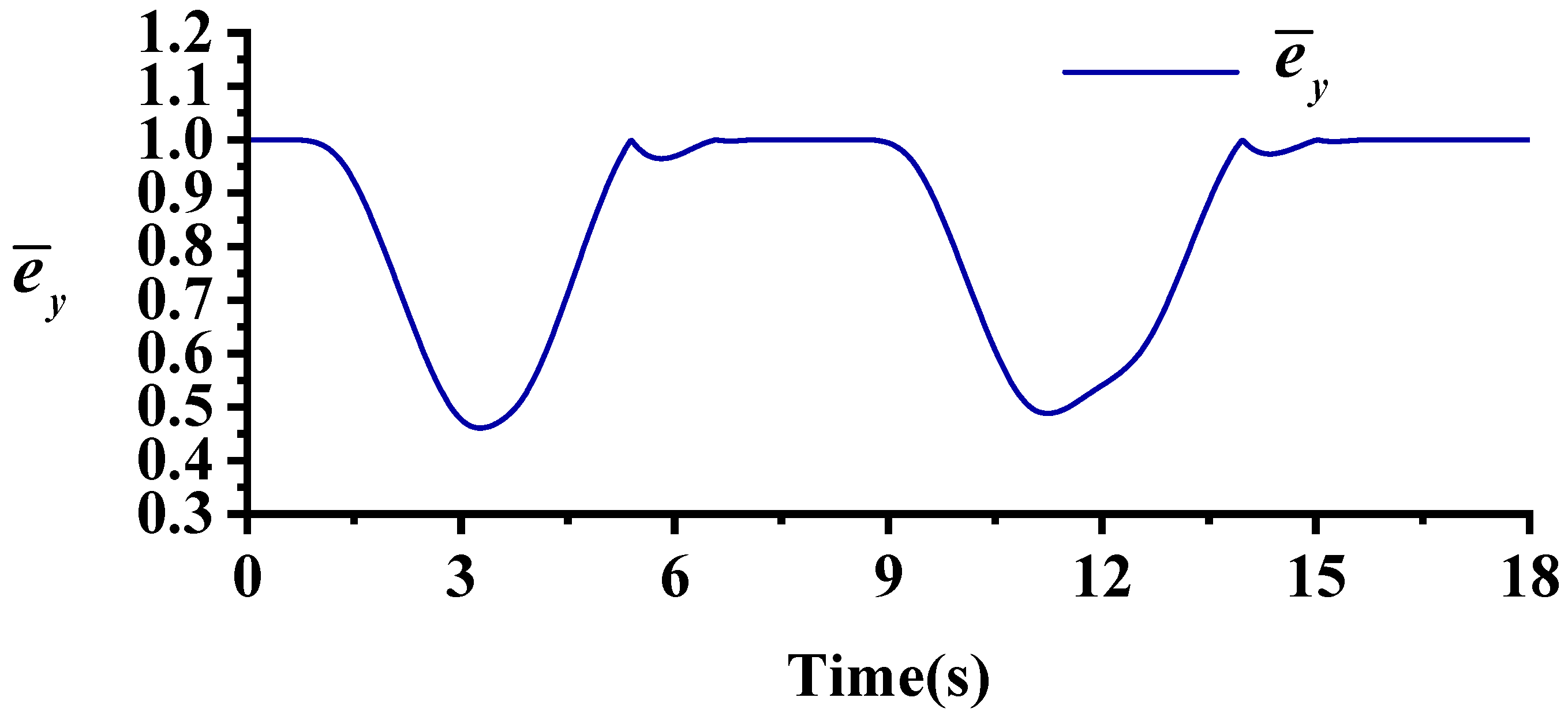
Comparing the simulation results in Figure 6 and Figure 7, in two cases with or without FLS, HAPF-FMPC has better control performance for static and low-speed obstacle avoidance. Path planning with HAPF-FMPC allows for a faster return to a smooth state of track. Figure 8, Figure 9 and Figure 10 shows the input and output of FLS, indicating the dynamic adjustment of HAPF-FMPC using FLS.

6.2. Adaptive Scheme

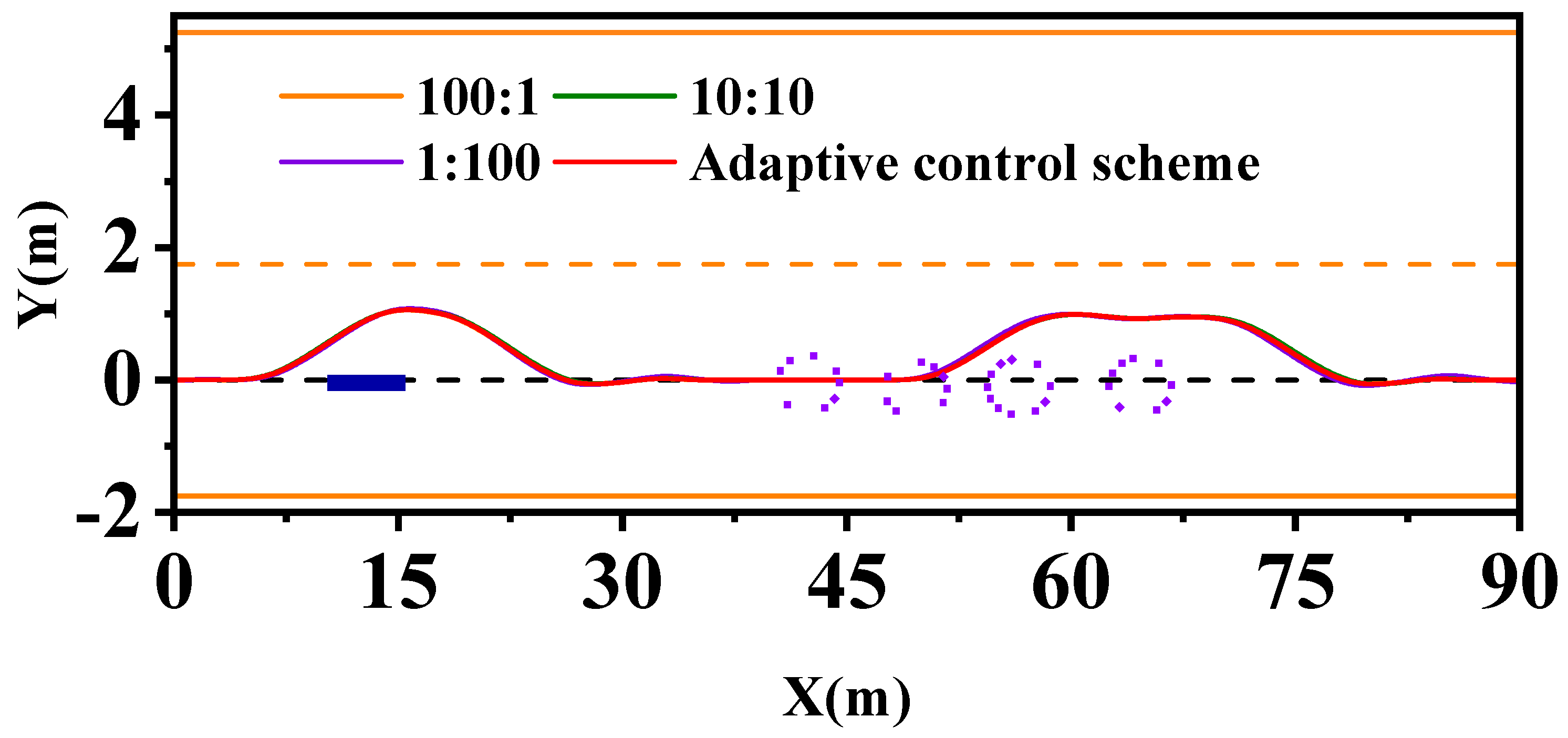
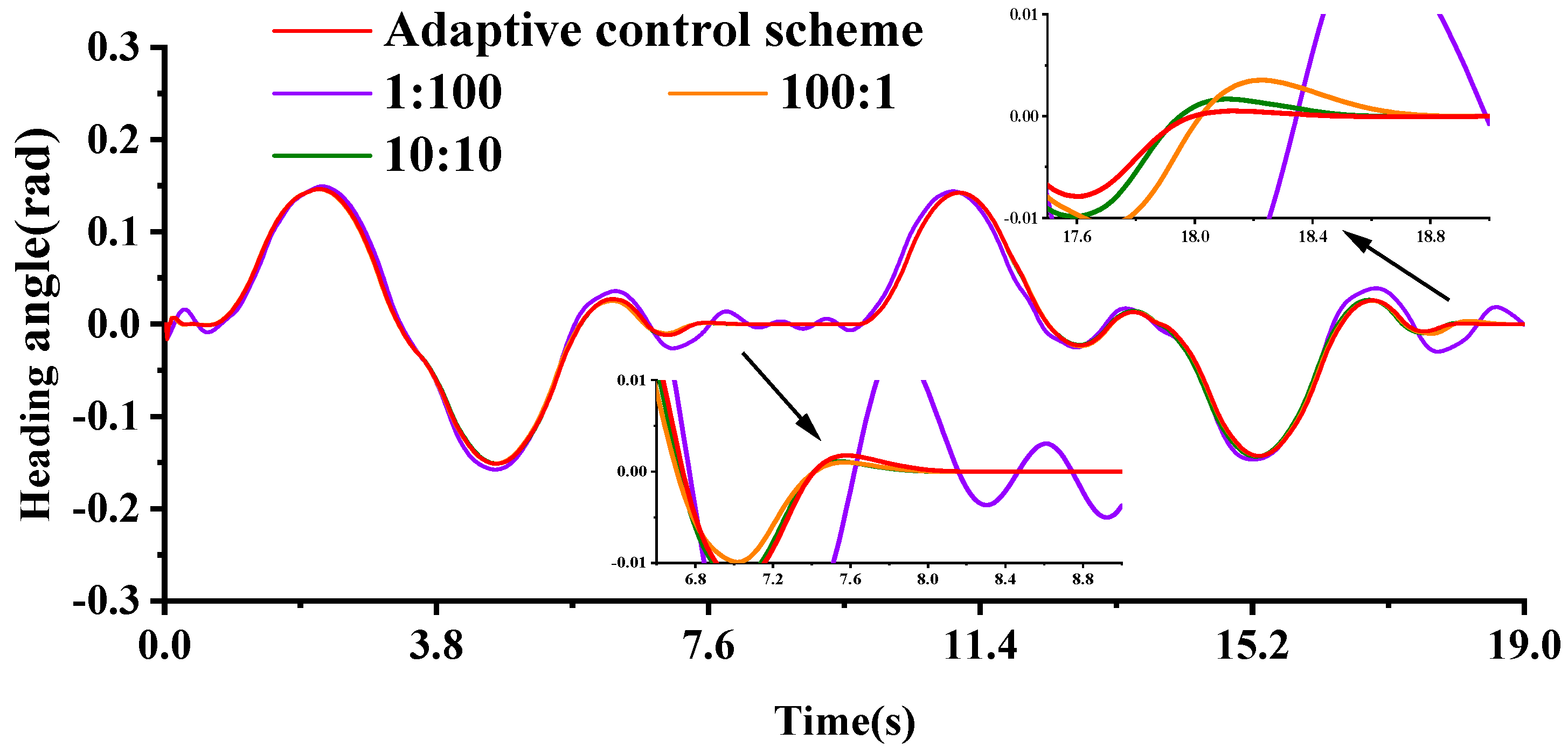
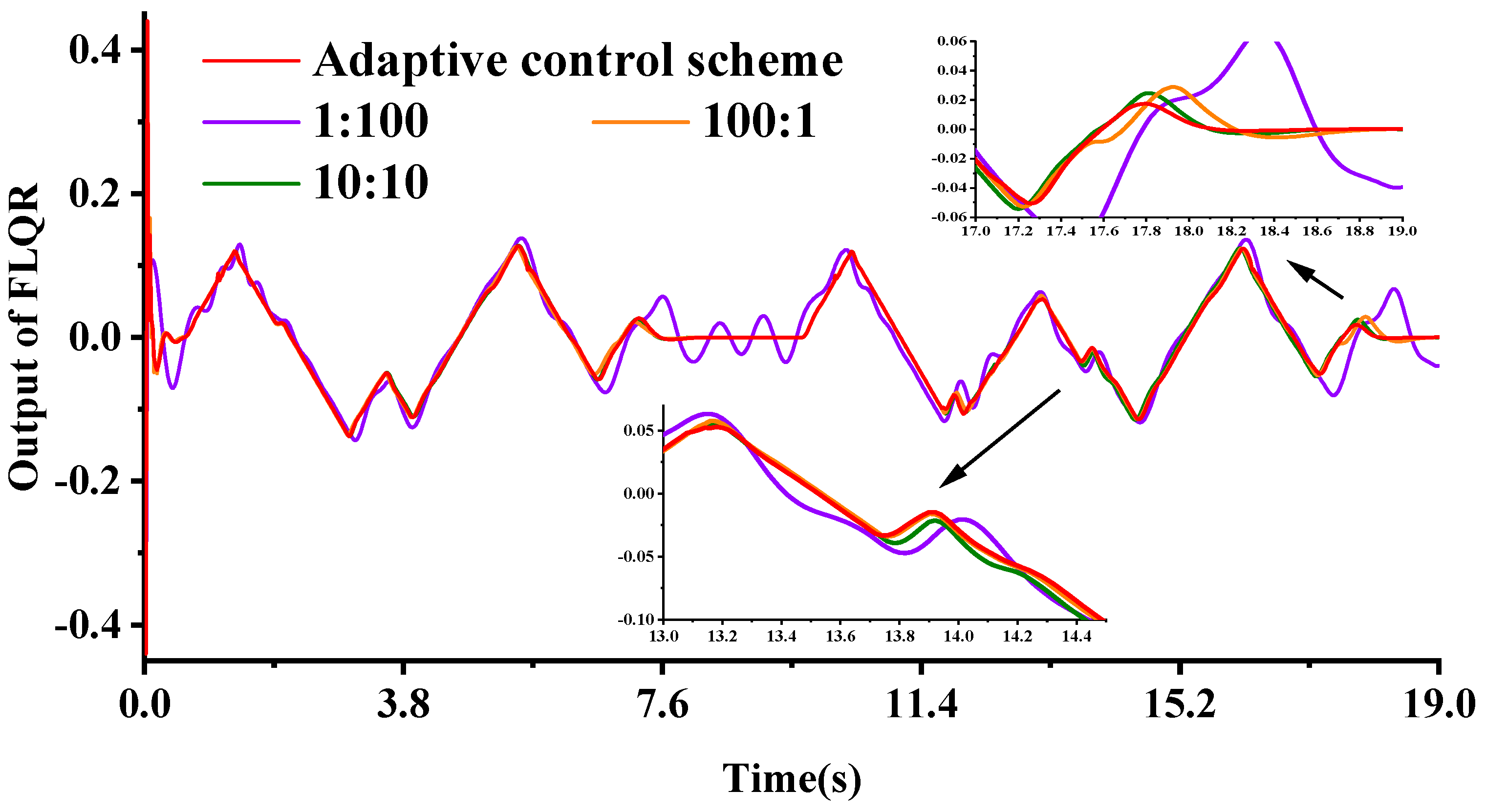
This scenario validates the efficacy of the adaptive scheme, as proposed in this study, for handling both dynamic and static obstacles. In addition, we compared the proposed scheme for lateral controllers equipped with FLS with a traditional LQR adjustment scheme. The AGV is travelling on a two-lane road with a single-lane width of 3.5 m. Scenario 2 has a static obstacle at x = 10 m. A dynamic obstacle travels at x = 40 m with a speed of 1.5 m/s. The following is a comparison between the adaptive scheme and the other LQR matching schemes (Q: R).

From Figure 11, Figure 12 and Figure 13, it can be seen that the adaptive control scheme proposed in this paper can complete path planning and trajectory tracking for static and dynamic obstacles during obstacle avoidance. In addition, the FLQR lateral controller can be seen to have a positive effect on the control performance of the AGV in terms of obstacle avoidance of dynamic obstacles. The feasibility of the optimisation scheme of the FLS proposed in this paper is demonstrated.

6.3. Obstacle Avoidance Deceleration

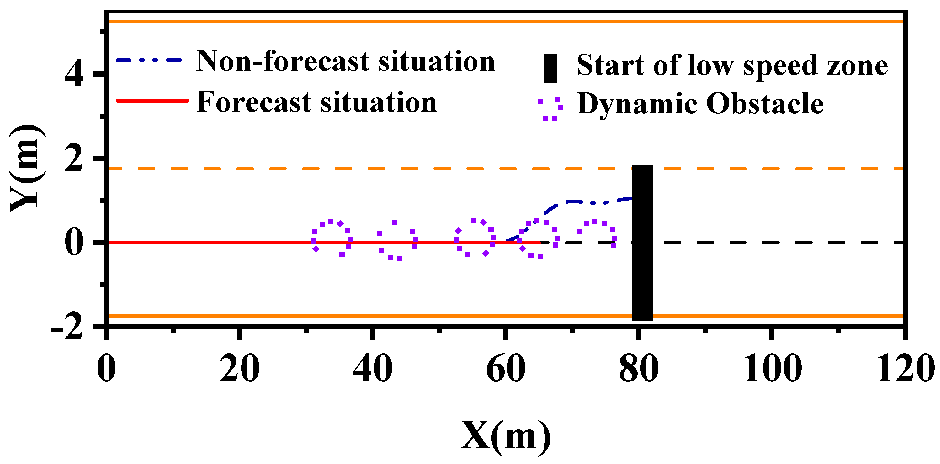
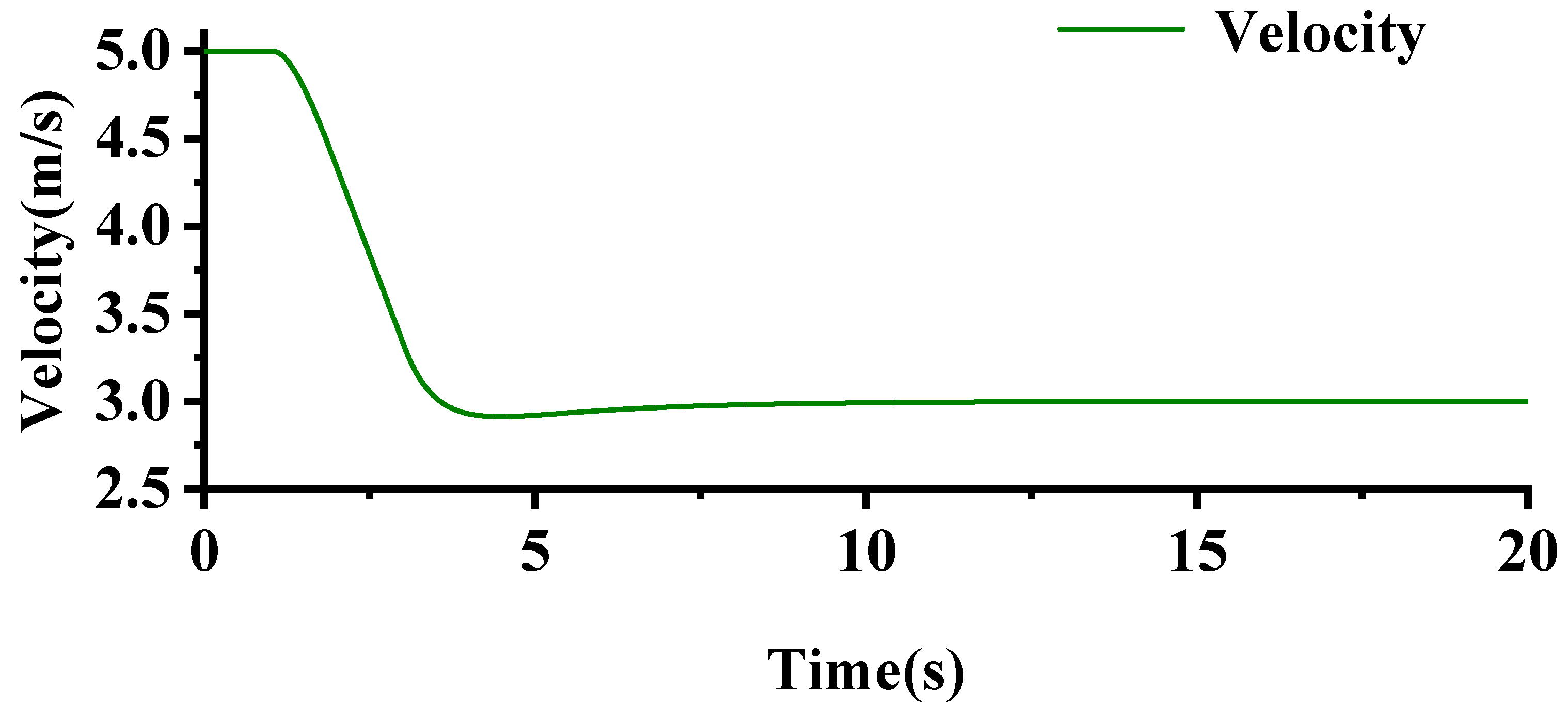
Scenario 3 is set up to demonstrate how the adaptive control scheme, based on information shared by the IVICS, determines that the HAPF-FMPC is not working and slows down to avoid the obstacle. Scenario 3 sets the low-speed zone to start at x = 80 m, which is unsuitable for obstacle avoidance. The AGV travels at 5 m/s at x = 0 m, and the dynamic obstacle travels at 3 m/s at x = 30 m. AGVs follow a dynamic obstacle deceleration strategy without avoiding obstacles. A comparison of the two options for performing speed planning and for performing path planning is shown below.

From Figure 14 and Figure 15, it can be seen from the simulation comparison results that the APF in the control scheme can be dynamically adjusted depending on the shared information from the IVICS. With a dynamically adjusted APF, the AGV can decelerate and follow when it is impossible to avoid obstacles. It can prevent AGVs from colliding with impenetrable obstacles or failing to decelerate in low-speed zones due to blind APF generation.

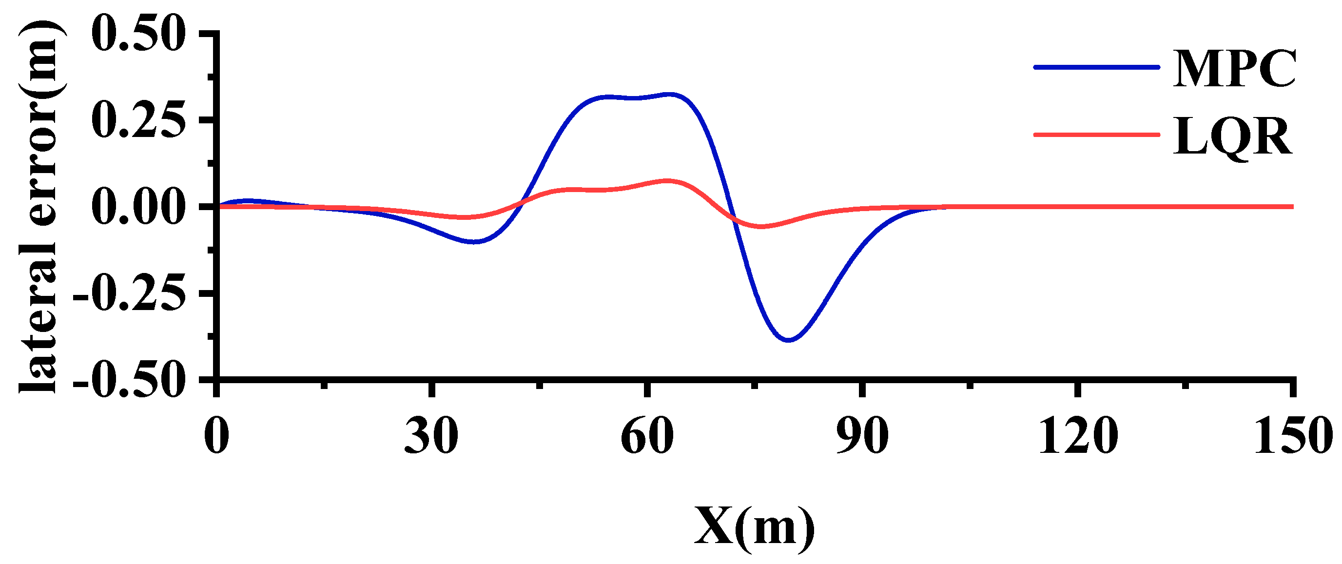
6.4. Controller Comparison

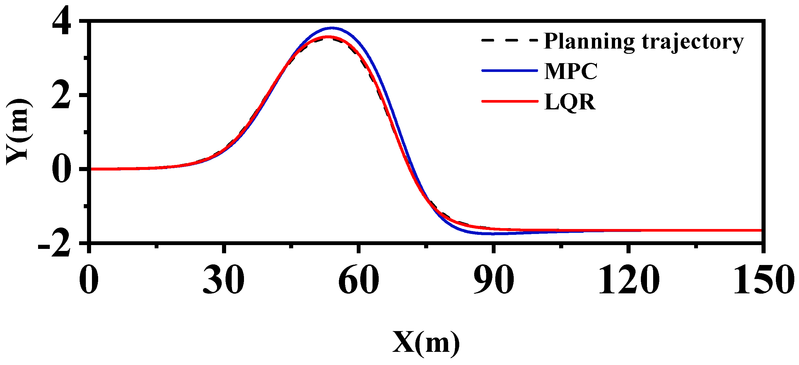
This paper presents a comparative analysis of two control methods, examining both their tracking effectiveness and runtime within an identical model. The goal is to ascertain the superiority of the proposed controller scheme. For the purpose of accurately simulating the controller within real-world applications, the controller’s weight values are modulated at the specific instance when x equals 5 m.

In real-time performance tests, the MPC method averaged 14.149451 s for ten times path tracing, whereas the LQR took only 1.2213301 s, marking an 91.368357% efficiency improvement. Additionally, the exceptional tracking performance of the LQR is further illustrated in Figure 16 and Figure 17. Specific experimental results are presented in

Table 6. Time required for computing with different controllers.

Method	Calculation Time(s)
MPC	15.8315	14.10677	13.96738	13.75368	14.03611	13.99712	13.99165	13.92399	13.85656	14.02974
LQR	1.311854	1.228484	1.210175	1.218449	1.217116	1.212055	1.23513	1.190204	1.191608	1.198226

.

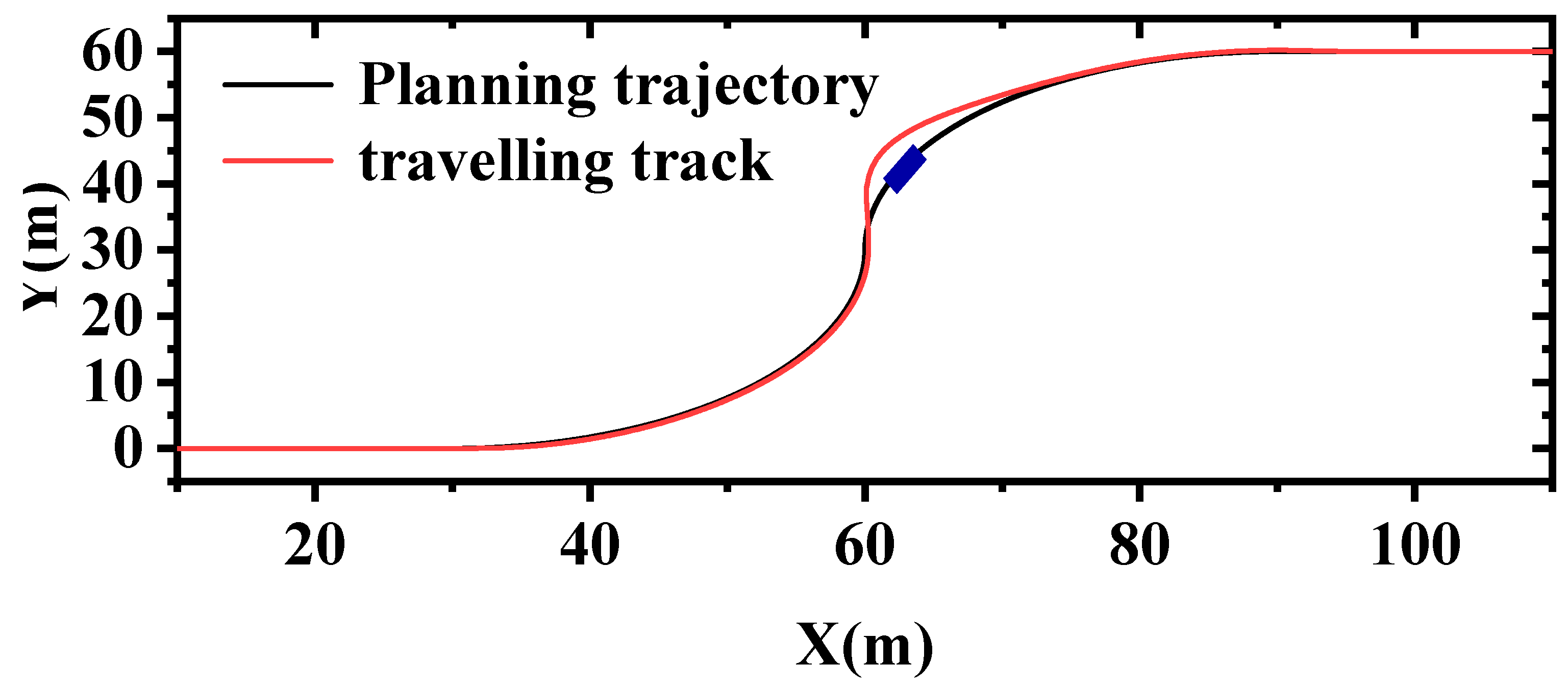
6.5. Turning Obstacle Avoidance Simulation for AGVs

In port settings, AGVs face conflicts and deadlocks not just in linear transport but also during turns. Especially in areas without lane lines, it is vital for AGVs to adeptly avoid obstacles. This study simulates an “S”-shaped path with static obstacles at (62,40) to demonstrate the effectiveness of our proposed scheme in handling turning manoeuvres (see Figure 18).

The simulation results show that effective path planning and trajectory tracking for obstacle avoidance in port environments using the strategy proposed in this study is feasible under specific conditions. The results validate the applicability of the proposed scheme in potential field applications.

7. Conclusions

In order to optimise the operation of automated terminals and cut down the occurrence of conflicts and deadlocks, this study uniquely uses a combination of MPC, FLS, and APF theories to develop a strategy for hierarchical path planning and trajectory tracking of AGVs. In our design, the novel APF guarantees high accuracy and tunability and successfully incorporates the cost function of MPC. Not to be overlooked, we use the FLS to dynamically adjust the weight factor of the cost function, which not only improves the ability of the AGV to return to the original path after obstacle avoidance but also enhances its stability. Further, we develop corresponding lateral and longitudinal controllers to track the pre-set path and speed accurately. In particular, the lateral tracker uses a dynamics model and the FLS to adjust the weights before each obstacle avoidance, significantly improving the control performance and tracking ability of the AGV. In cases where obstacle avoidance is not possible, we reduce the speed of the AGV with velocity planning and thus avoid conflict. The simulation results demonstrate the superiority of our proposed control scheme in path planning and trajectory tracking. In conclusion, regarding path planning, the integration of MPC, APF, and FLS enhances the ability to swiftly return to the original trajectory in AGV path planning. In terms of tracking control, the combination of the LQR and FLS improves the AGV’s adaptive adjustment capabilities in tracking the obstacle avoidance path.

However, given the intricate demands of dock loading, precise AGV modelling is crucial. In future work, we aim to refine our AGV modelling, considering the challenges of tracking and planning during heavy unloading in ports. Our goal is to further enhance the efficiency and safety of automated terminal operations during the horizontal transport phase.

References

- Chen, X.; Wang, Z.; Hua, Q.; Shang, W.-L.; Luo, Q.; Yu, K. AI-Empowered Speed Extraction via Port-Like Videos for Vehicular Trajectory Analysis. IEEE Trans. Intell. Transport. Syst. 2023, 24, 4541–4552. [Google Scholar] [CrossRef]
- He, J.; Xiao, X.; Yu, H.; Zhang, Z. Dynamic Yard Allocation for Automated Container Terminal. Ann. Oper. Res. 2022. [Google Scholar] [CrossRef]
- Zhong, M.; Yang, Y.; Dessouky, Y.; Postolache, O. Multi-AGV Scheduling for Conflict-Free Path Planning in Automated Container Terminals. Comput. Ind. Eng. 2020, 142, 106371. [Google Scholar] [CrossRef]
- Hu, H.; Yang, X.; Xiao, S.; Wang, F. Anti-Conflict AGV Path Planning in Automated Container Terminals Based on Multi-Agent Reinforcement Learning. Int. J. Prod. Res. 2023, 61, 65–80. [Google Scholar] [CrossRef]
- Quan, Y.; Lei, M.; Chen, W.; Wang, R. AGV Motion Balance and Motion Regulation Under Complex Conditions. Int. J. Control Autom. Syst. 2022, 20, 551–563. [Google Scholar] [CrossRef]
- Akopov, A.S.; Beklaryan, L.A.; Beklaryan, A.L. Simulation-Based Optimisation for Autonomous Transportation Systems Using a Parallel Real-Coded Genetic Algorithm with Scalable Nonuniform Mutation. Cybern. Inf. Technol. 2021, 21, 127–144. [Google Scholar] [CrossRef]
- Nikolos, I.K.; Valavanis, K.P.; Tsourveloudis, N.C.; Kostaras, A.N. Evolutionary Algorithm Based Offline/Online Path Planner for Uav Navigation. IEEE Trans. Syst. Man Cybern. B 2003, 33, 898–912. [Google Scholar] [CrossRef]
- Kim, J.; Yang, G.-H. Improvement of Dynamic Window Approach Using Reinforcement Learning in Dynamic Environments. Int. J. Control Autom. Syst. 2022, 20, 2983–2992. [Google Scholar] [CrossRef]
- Lee, D.H.; Lee, S.S.; Ahn, C.K.; Shi, P.; Lim, C.-C. Finite Distribution Estimation-Based Dynamic Window Approach to Reliable Obstacle Avoidance of Mobile Robot. IEEE Trans. Ind. Electron. 2021, 68, 9998–10006. [Google Scholar] [CrossRef]
- Han, S.; Wang, L.; Wang, Y.; He, H. A Dynamically Hybrid Path Planning for Unmanned Surface Vehicles Based on Non-Uniform Theta* and Improved Dynamic Windows Approach. Ocean Eng. 2022, 257, 111655. [Google Scholar] [CrossRef]
- Magyar, B.; Tsiogkas, N.; Deray, J.; Pfeiffer, S.; Lane, D. Timed-Elastic Bands for Manipulation Motion Planning. IEEE Robot. Autom. Lett. 2019, 4, 3513–3520. [Google Scholar] [CrossRef]
- Sun, X.; Deng, S.; Zhao, T.; Tong, B. Motion Planning Approach for Car-like Robots in Unstructured Scenario. Trans. Inst. Meas. Control 2022, 44, 754–765. [Google Scholar] [CrossRef]
- Wang, Z.; Shen, Y.; Zhang, L.; Zhang, S.; Zhou, Y. Towards Robust Autonomous Coverage Navigation for Carlike Robots. IEEE Robot. Autom. Lett. 2021, 6, 8742–8749. [Google Scholar] [CrossRef]
- Xie, S.; Hu, J.; Bhowmick, P.; Ding, Z.; Arvin, F. Distributed Motion Planning for Safe Autonomous Vehicle Overtaking via Artificial Potential Field. IEEE Trans. Intell. Transport. Syst. 2022, 23, 21531–21547. [Google Scholar] [CrossRef]
- Zhen, Q.; Wan, L.; Li, Y.; Jiang, D. Formation Control of a Multi-AUVs System Based on Virtual Structure and Artificial Potential Field on SE(3). Ocean Eng. 2022, 253, 111148. [Google Scholar] [CrossRef]
- Zhang, G.; Han, J.; Li, J.; Zhang, X. APF-Based Intelligent Navigation Approach for USV in Presence of Mixed Potential Directions: Guidance and Control Design. Ocean Eng. 2022, 260, 111972. [Google Scholar] [CrossRef]
- Huang, Z.; Wu, Q.; Ma, J.; Fan, S. An APF and MPC Combined Collaborative Driving Controller Using Vehicular Communication Technologies. Chaos Solitons Fractals 2016, 89, 232–242. [Google Scholar] [CrossRef]
- Zuo, Z.; Yang, X.; Li, Z.; Wang, Y.; Han, Q.; Wang, L.; Luo, X. MPC-Based Cooperative Control Strategy of Path Planning and Trajectory Tracking for Intelligent Vehicles. IEEE Trans. Intell. Veh. 2021, 6, 513–522. [Google Scholar] [CrossRef]
- Liu, Z.; Yuan, X.; Huang, G.; Wang, Y.; Zhang, X. Two Potential Fields Fused Adaptive Path Planning System for Autonomous Vehicle under Different Velocities. ISA Trans. 2021, 112, 176–185. [Google Scholar] [CrossRef]
- Wang, X.; Liu, J.; Peng, H.; Qie, X.; Zhao, X.; Lu, C. A Simultaneous Planning and Control Method Integrating APF and MPC to Solve Autonomous Navigation for USVs in Unknown Environments. J. Intell. Robot. Syst. 2022, 105, 36. [Google Scholar] [CrossRef]
- De Ryck, M.; Versteyhe, M.; Debrouwere, F. Automated Guided Vehicle Systems, State-of-the-Art Control Algorithms and Techniques. J. Manuf. Syst. 2020, 54, 152–173. [Google Scholar] [CrossRef]
- Arslan, M.S.; Sever, M. Vehicle Stability Enhancement and Rollover Prevention by a Nonlinear Predictive Control Method. Trans. Inst. Meas. Control 2019, 41, 2135–2149. [Google Scholar] [CrossRef]
- Guo, L.; Xu, H.; Zou, J.; Jie, H.; Zheng, G. Variable Gain Control-Based Acceleration Slip Regulation Control Algorithm for Four-Wheel Independent Drive Electric Vehicle. Trans. Inst. Meas. Control 2021, 43, 902–914. [Google Scholar] [CrossRef]
- Liu, W.; Liu, P.; Yu, Y.; Zhang, Q.; Wan, Y.; Wang, M. Optimal Torque Distribution of Distributed Driving AGV under the Condition of Centroid Change. Sci. Rep. 2021, 11, 21404. [Google Scholar] [CrossRef] [PubMed]
- Shi, Q.; Zhang, H. Road-Curvature-Range-Dependent Path Following Controller Design for Autonomous Ground Vehicles Subject to Stochastic Delays. IEEE Trans. Intell. Transport. Syst. 2022, 23, 17440–17450. [Google Scholar] [CrossRef]
- Wu, Y.; Wang, L.; Zhang, J.; Li, F. Path Following Control of Autonomous Ground Vehicle Based on Nonsingular Terminal Sliding Mode and Active Disturbance Rejection Control. IEEE Trans. Veh. Technol. 2019, 68, 6379–6390. [Google Scholar] [CrossRef]
- Zhang, H.; Li, B.; Xiao, B.; Yang, Y.; Ling, J. Nonsingular Recursive-Structure Sliding Mode Control for High-Order Nonlinear Systems and an Application in a Wheeled Mobile Robot. ISA Trans. 2022, 130, 553–564. [Google Scholar] [CrossRef]
- Li, B.; Zhang, H.; Xiao, B.; Wang, C.; Yang, Y. Fixed-Time Integral Sliding Mode Control of a High-Order Nonlinear System. Nonlinear Dyn. 2022, 107, 909–920. [Google Scholar] [CrossRef]
- Eckert, J.J.; Barbosa, T.P.; Silva, F.L.; Roso, V.R.; Silva, L.C.A.; da Silva, L.A.R. Optimum Fuzzy Logic Controller Applied to a Hybrid Hydraulic Vehicle to Minimize Fuel Consumption and Emissions. Expert. Syst. Appl. 2022, 207, 117903. [Google Scholar] [CrossRef]
- Qazani, M.R.C.; Asadi, H.; Mohamed, S.; Lim, C.P.; Nahavandi, S. An Optimal Washout Filter for Motion Platform Using Neural Network and Fuzzy Logic. Eng. Appl. Artif. Intell. 2022, 108, 104564. [Google Scholar] [CrossRef]
- Liao, Y.; Jiang, Q.; Du, T.; Jiang, W. Redefined Output Model-Free Adaptive Control Method and Unmanned Surface Vehicle Heading Control. IEEE J. Ocean Eng. 2020, 45, 714–723. [Google Scholar] [CrossRef]
- Shin, J.; Kwak, D.; Kwak, K. Model Predictive Path Planning for an Autonomous Ground Vehicle in Rough Terrain. Int. J. Control Autom. Syst. 2021, 19, 2224–2237. [Google Scholar] [CrossRef]
- Yang, W.; Liang, J.; Yang, J.; Walker, P.D.; Zhang, N. Corresponding Drivability Control and Energy Control Strategy in Uninterrupted Multi-Speed Mining Trucks. J. Frankl. Inst. 2021, 358, 1214–1239. [Google Scholar] [CrossRef]
- Tanveer, A.; Ahmad, S.M. High Fidelity Modelling and GA Optimized Control of Yaw Dynamics of a Custom Built Remotely Operated Unmanned Underwater Vehicle. Ocean Eng. 2022, 266, 112836. [Google Scholar] [CrossRef]
- Chalak Qazani, M.R.; Asadi, H.; Mohamed, S.; Lim, C.P.; Nahavandi, S. A Time-Varying Weight MPC-Based Motion Cueing Algorithm for Motion Simulation Platform. IEEE Trans. Intell. Transport. Syst. 2022, 23, 11767–11778. [Google Scholar] [CrossRef]
- Wang, F.; Li, J.; Li, Z.; Ke, D.; Du, J.; Garcia, C.; Rodriguez, J. Design of Model Predictive Control Weighting Factors for PMSM Using Gaussian Distribution-Based Particle Swarm Optimization. IEEE Trans. Ind. Electron. 2022, 69, 10935–10946. [Google Scholar] [CrossRef]
- Sir Elkhatem, A.; Naci Engin, S. Robust LQR and LQR-PI Control Strategies Based on Adaptive Weighting Matrix Selection for a UAV Position and Attitude Tracking Control. Alex. Eng. J. 2022, 61, 6275–6292. [Google Scholar] [CrossRef]
- Lu, Y.; Khajepour, A.; Soltani, A.; Li, R.; Zhen, R.; Liu, Y.; Wang, M. Gain-Adaptive Skyhook-LQR: A Coordinated Controller for Improving Truck Cabin Dynamics. Control Eng. Pract. 2023, 130, 105365. [Google Scholar] [CrossRef]
- Gong, J.; Jiang, Y.; Xu, W. Model Predictive Control for Self-Driving Vehicles, 2nd ed.; Beijing Institute of Technology Press: Beijing, China, 2014; ISBN 978-7-5682-8232-1. [Google Scholar]
- Azzabi, A.; Nouri, K. An Advanced Potential Field Method Proposed for Mobile Robot Path Planning. Trans. Inst. Meas. Control 2019, 41, 3132–3144. [Google Scholar] [CrossRef]
- Shi, Z.; Jiang, H.; Yu, W.; Liu, Y.; Jiang, X.; Jiang, M. Research on Adaptive MPC Algorithm for Path Tracking Control. Comput. Eng. Appl. 2020, 56, 6. [Google Scholar] [CrossRef]
- Yang, T.; Bai, Z.; Li, Z.; Feng, N.; Chen, L. Intelligent Vehicle Lateral Control Method Based on Feedforward + Predictive LQR Algorithm. Actuators 2021, 10, 228. [Google Scholar] [CrossRef]
Figure 1.
Hierarchical logic for vehicle obstacle avoidance.
Figure 2.
The conflicts and deadlocks of AGVs in automated terminals.
Figure 3.
Framework for an obstacle avoidance solution for AGV.
Figure 4.
AGV kinematic model.
Figure 5.
AGV dynamics model.
Figure 6.
Path of HAPF-FMPC and HAPF-MPC in obstacle avoidance for static and dynamic obstacles.
Figure 7.
Heading angle variation curves under two control schemes of HAPF-FMPC and HAPF-MPC.
Figure 8.
The curve of the FLS input .
Figure 9.
Figure 10.
The curve of the FLS output .
Figure 11.
Driving paths for dynamic and static obstacles with different LQR rationing schemes.
Figure 12.
Heading angles of dynamic and static obstacles for different LQR rationing schemes.
Figure 13.
Front-wheel turning angles for dynamic and static obstacles with different LQR proportioning schemes.
Figure 14.
Comparative schematic diagram of whether speed planning is followed in the case of unavoidable obstacles.
Figure 15.
AGV speed profile after speed planning without obstacle avoidance.
Figure 16.
Path tracking effect with different controllers.
Figure 17.
Lateral error of path tracking with different controllers.
Figure 18.
Obstacle avoidance routes under curved paths.