
A Comparative Feasibility Study of the Use of Hydrogen Produced from Surplus Wind Power for a Gas Turbine Combined Cycle Power Plant

1
Graduate School, Inha University, 100 Inha-ro, Michuhol-gu, Incheon 22212, Korea
2
Department of Mechanical Engineering, Inha University, 100 Inha-ro, Michuhol-gu, Incheon 22212, Korea
*
Author to whom correspondence should be addressed.
Energies 2021, 14(24), 8342; https://doi.org/10.3390/en14248342
Submission received: 6 November 2021
/
Revised: 26 November 2021
/
Accepted: 1 December 2021
/
Published: 10 December 2021
(This article belongs to the Special Issue Advances in Gas Turbine Performance, Heat Transfer and Aerodynamics)
Abstract
:Because of the increasing challenges raised by climate change, power generation from renewable energy sources is steadily increasing to reduce greenhouse gas emissions, especially CO2. However, this has escalated concerns about the instability of the power grid and surplus power generated because of the intermittent power output of renewable energy. To resolve these issues, this study investigates two technical options that integrate a power-to-gas (PtG) process using surplus wind power and the gas turbine combined cycle (GTCC). In the first option, hydrogen produced using a power-to-hydrogen (PtH) process is directly used as fuel for the GTCC. In the second, hydrogen from the PtH process is converted into synthetic natural gas by capturing carbon dioxide from the GTCC exhaust, which is used as fuel for the GTCC. An annual operational analysis of a 420-MW-class GTCC was conducted, which shows that the CO2 emissions of the GTCC-PtH and GTCC-PtM plants could be reduced by 95.5% and 89.7%, respectively, in comparison to a conventional GTCC plant. An economic analysis was performed to evaluate the economic feasibility of the two plants using the projected cost data for the year 2030, which showed that the GTCC-PtH would be a more viable option.
1. Introduction
Driven by the increased worldwide attention to the challenges raised by climate change, greenhouse gas mitigation has become an important task in all industrial fields. Efforts are being made to reduce the amount of power generated from conventional power generation systems and to increase the power generation ratio of renewable energy to mitigate emissions [1]. Unlike conventional methods that use fossil fuels, renewable energy sources such as wind and solar power do not emit , so they can significantly contribute to the resolution of climate change challenges [2,3].
By 2023–25, the annual increase in the global offshore wind power generation is forecast to be double the levels in 2020, and the annual growth of solar power generation is projected to reach 130–165 GW [4]. If this trend is maintained, the ratio of solar power and wind power generation is expected to outweigh those of natural gas (NG) power generation by 2023 and coal thermal power generation by 2024 [4]. However, while conventional fossil fuel power plants can supply stable power to the electric grid, renewable energy suffers from the disadvantage of being intermittent.
Therefore, solar power and wind power are called variable renewable energy (VRE) sources. The critical issue with the variable nature of renewable energy is that there could be a large gap between the power supply and demand, which would act as a critical source of instability and might cause a catastrophic problem with the electric grid [5]. Accordingly, there is an urgent need to find a way to use the surplus power generated during times when power supplied by renewable sources is greater than the power demand [6], which would then be stably supplied when the power demand rapidly increases. The aim of this study is to find such a solution.
The gas turbine combined cycle (GTCC) with NG has become one of the main sources of power generation in the past few decades because of its high thermal efficiency, eco-friendliness, fast mobility, and strong load-following capability. A considerable number of GTCC power plants are contributing to the stable operation of the power grid. This is done through either peak-cut operation or a type of cyclic operation, such as daily start and stop operation (DSS). The advantages include fast mobility and strong load-following capability [7]. As the share of VRE increases, a flexible power generation source is required to compensate for the variability, and the GTCC is expected to be the best option. However, the GTCC is not free from the problem of emitting either, because it uses NG as fuel. Therefore, the GTCC’s emissions problem also needs to be resolved to achieve the goal of resolving the challenges of climate change through greenhouse gas mitigation [8].
One of the methods to reduce the total emissions is to use an energy storage system (ESS). An ESS resolves the instability problem of the power grid resulting from the variability of renewable energy and improves the discord between the power demand and supply by storing surplus power generated by renewable energy and releasing it when the power demand is high. This reduces the use of fossil fuels and consequently decreases the overall emissions.
Although the simplest and most representative ESS method is electrochemical energy storage using batteries, several other ESS systems are available. Pumped hydro is a conventional large-scale ESS. Compressed air energy storage (CAES) is a method to store energy in the form of high-pressure air, and a modified method stores air in the form of liquid to increase the energy storage density. Another important method that has been gaining attention lately is chemical energy storage, where surplus power is used to generate hydrogen through water electrolysis [9].
Chemical energy storage has a higher energy density and less energy loss than electrochemical storage, so it enables long-term storage [10]. An ESS method of storing and using hydrogen by applying the chemical energy storage technique is called a power-to-gas (PtG) method. PtG methods have been receiving substantial attention lately as a means of next-generation energy storage because they can convert surplus power generated by renewable energy systems into and store it. Moreover, the conversion efficiency is expected to increase steadily, and the cost is expected to decrease steadily as a result of continuous research and development [11].
PtG methods are classified as power-to-hydrogen (PtH) and power-to-methane (PtM) methods based on how the hydrogen produced is used. PtH is a method of directly using the as fuel for a power generator such as a gas turbine (GT). Hydrogen may be combusted after mixing it with NG or as pure hydrogen depending on the technical readiness of the combustor [12]. Of course, a full revision of the combustor is required due to the differences in combustion characteristics between burning NG and hydrogen [13].
However, using hydrogen has the advantage of addressing the problem of greenhouse gas emissions while using an existing GTCC system. Thus, research on this technique is actively being performed in various countries and by various companies [14]. General Electric has developed an 82-MW-class GT that can use a maximum mole ratio of 90% in the case of co-firing with NG [15]. Siemens has successfully tested a 50-MW-class GT that can operate with an mole ratio of 50% [16].
With PtM, the hydrogen generated from the PtG process is reacted with carbon dioxide to produce synthetic NG (SNG) [17]. Just as with the PtH process, research is being carried out on the industrialization of the PtM process [18]. The thermophysical properties of SNG are very similar to those of NG, which allow it to be injected into an NG grid. However, a more practical option for on-site SNG production might be to use it directly for power generation. One option is to combine a GTCC plant with the PtM process, where the required for SNG production could be captured from the exhaust gas, and the produced SNG can be used as a fuel for the GT [19].
Many studies have attempted to combine PtG technology with VRE and GTCC systems. A study was conducted on combining wind power and PtG technology [20]. Various PtM and GTCC combination models have been studied [21], and a combination of wind power, PtM, and gas-fired power plants (GFPPs) was presented [22]. A combination of wind power, PtG (PtH, PtM), and thermal power plants (coal, gas) was also studied [23], but the GTCC was simulated using simple mathematical formulas instead of physical modeling and the hydrogen co-firing ratio was limited.
There have been numerous studies on power plant models that could store surplus power generated from VRE in an ESS and use it for power grid stabilization. However, there are still unverified aspects that require detailed investigations. In particular, a critical comparison of the PtH and PtM processes is required from the viewpoint of using them as a measure to achieve grid stabilization and the minimization of emissions. For example, large grid-scale power plants combined with PtH and PtM systems should be modeled, and then, their performance should be comparatively investigated to evaluate the feasibility of using these combinations in a practical power grid. In addition, it is critical to conduct a thermo-economic evaluation of the integration of VRE, PtG (PtH or PtM), and GTCC systems in consideration of the annual working conditions of the VRE and GTCC. The aim of this study was to accomplish this task, which has not been attempted before.
The goal of this study was to examine the feasibility of linking a 4-GW-class offshore wind farm and a 400-MW-class GTCC plant using PtG technology. The focus was on the comparison of the thermo-economic performance of the GTCC-PtH and GTCC-PtM technologies. First, a comparative analysis on the thermodynamic performance and emissions of GTCC-PtH and GTCC-PtM systems was carried out using the design conditions of the GTCC. The hydrogen mixing ratio in the GTCC combustor was the major variable. Second, the annual performance and emissions were analyzed in consideration of the variations in the wind power generation capability and power demand of the GTCC. Third, the economic feasibility was predicted using a cost scenario for the year 2030.
2. Configuration and Modeling
2.1. Case Definition
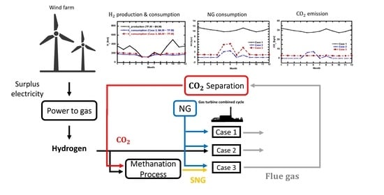
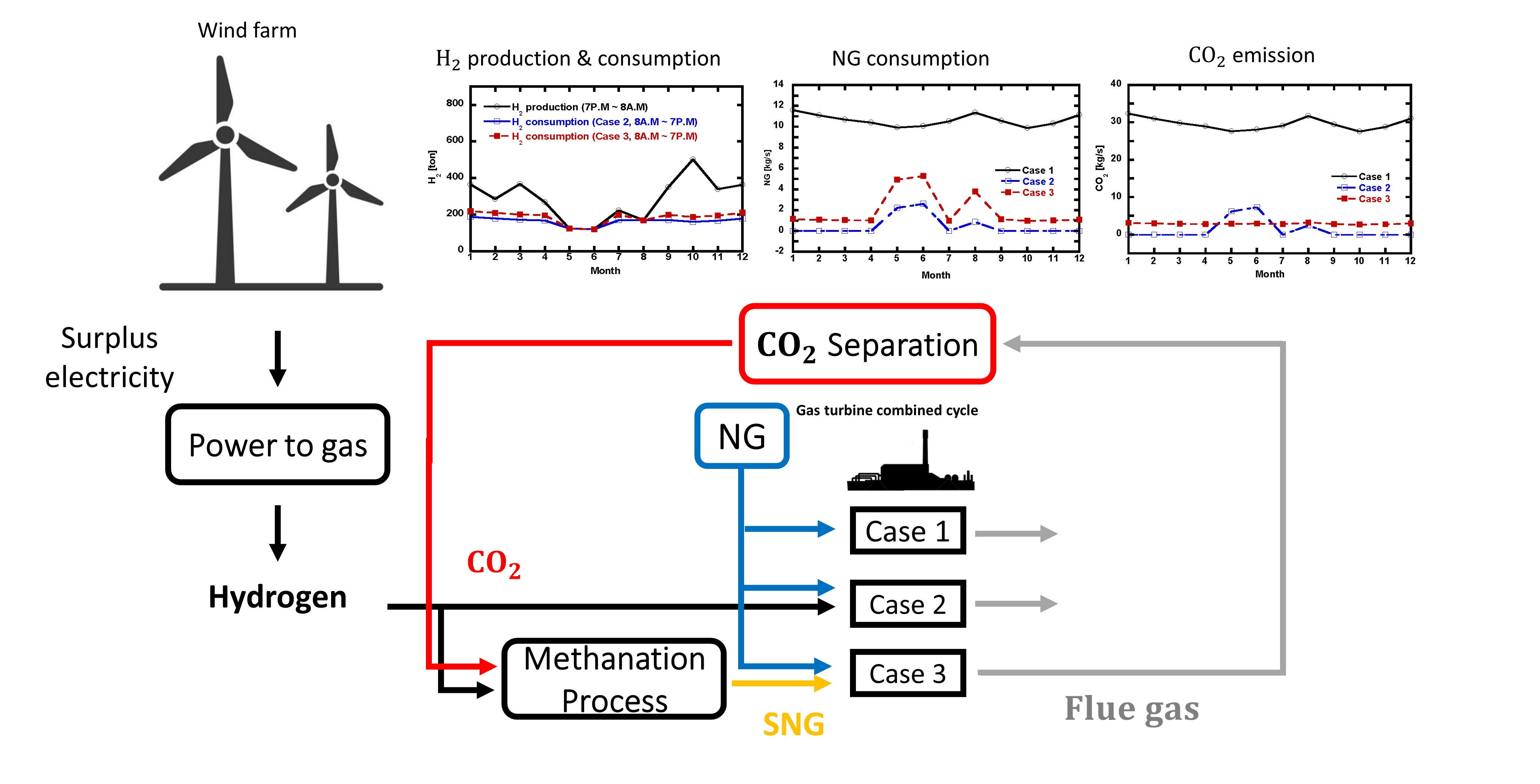
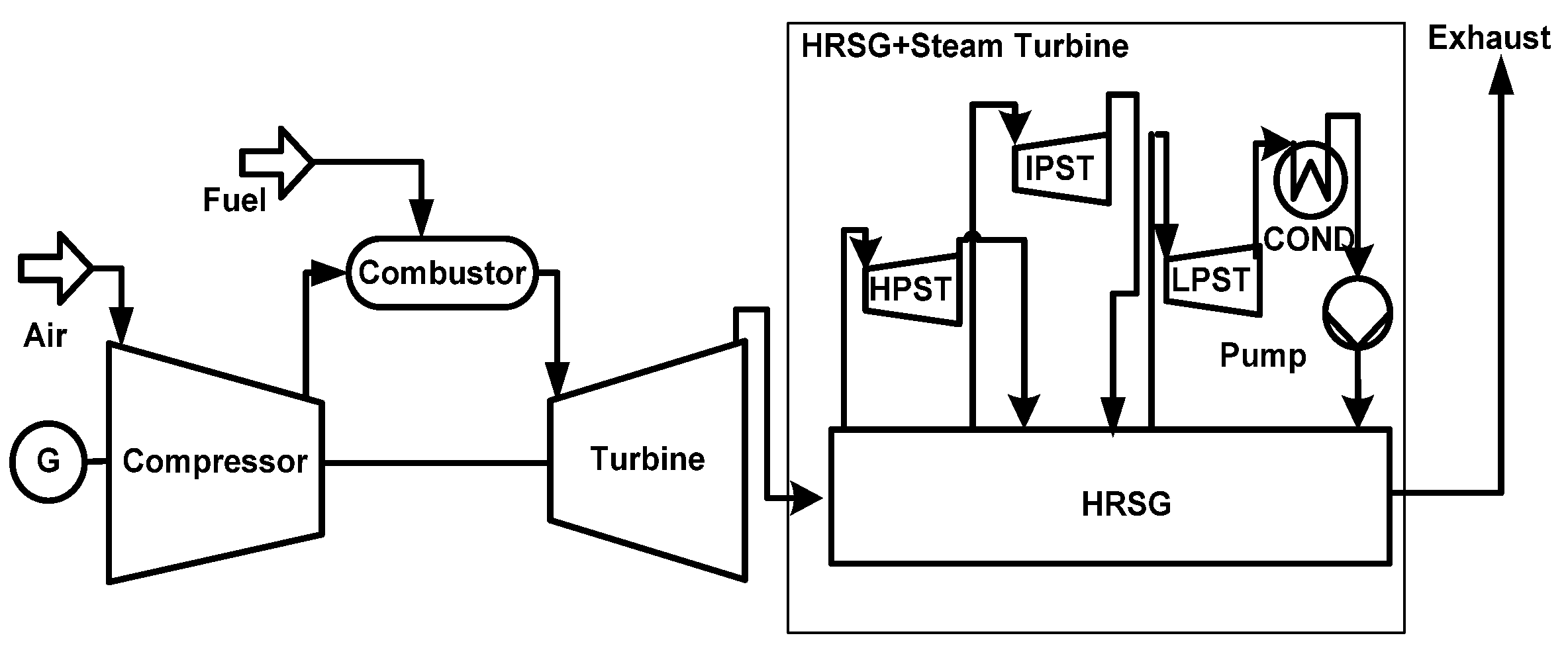
This study compared the system efficiencies, NG usages, and mitigation effects of three cases, which are defined in Table 1. Case 1 is a conventional GTCC, Case 2 integrates GTCC and PtH technologies, and Case 3 integrates GTCC and PtM technologies. The PtH process was modeled to produce 20.833 kg of per MWh of power based on a literature review [24]. The GTCC system was based on a 283-MW-class commercial GT [25], and a triple-pressure heat recovery system was used for its bottoming steam turbine cycle.
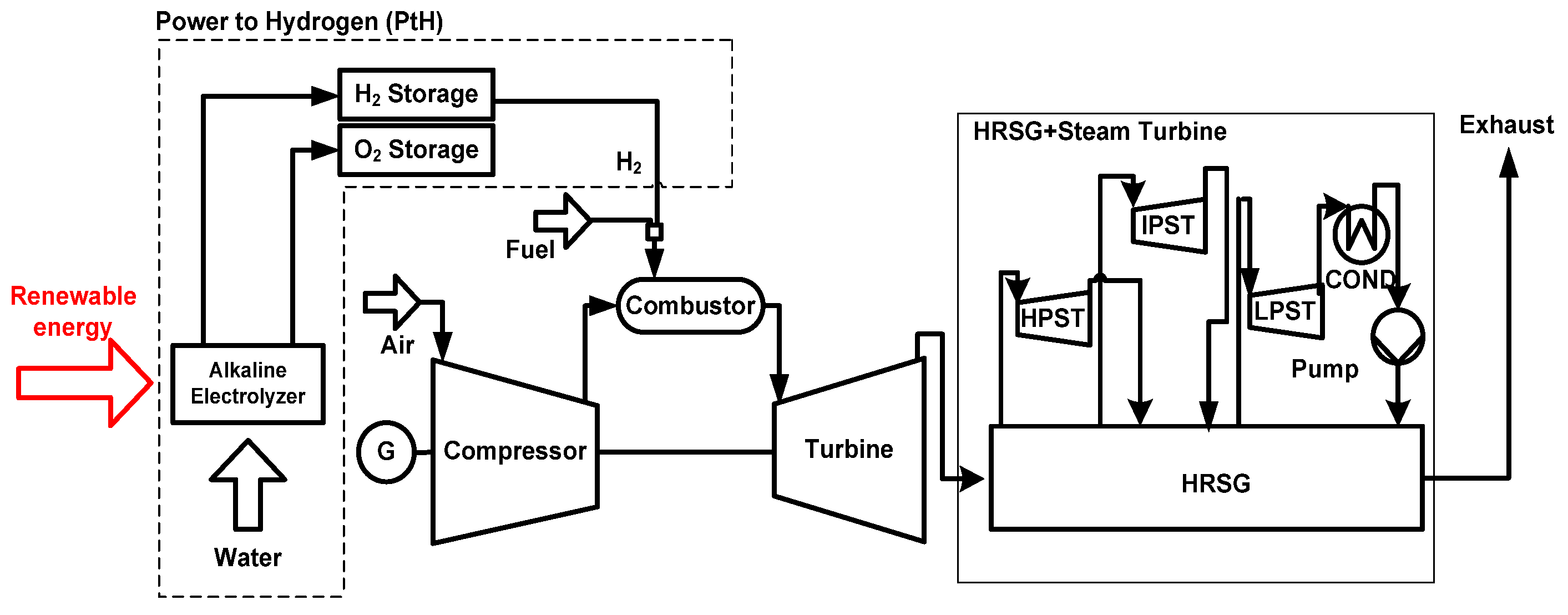
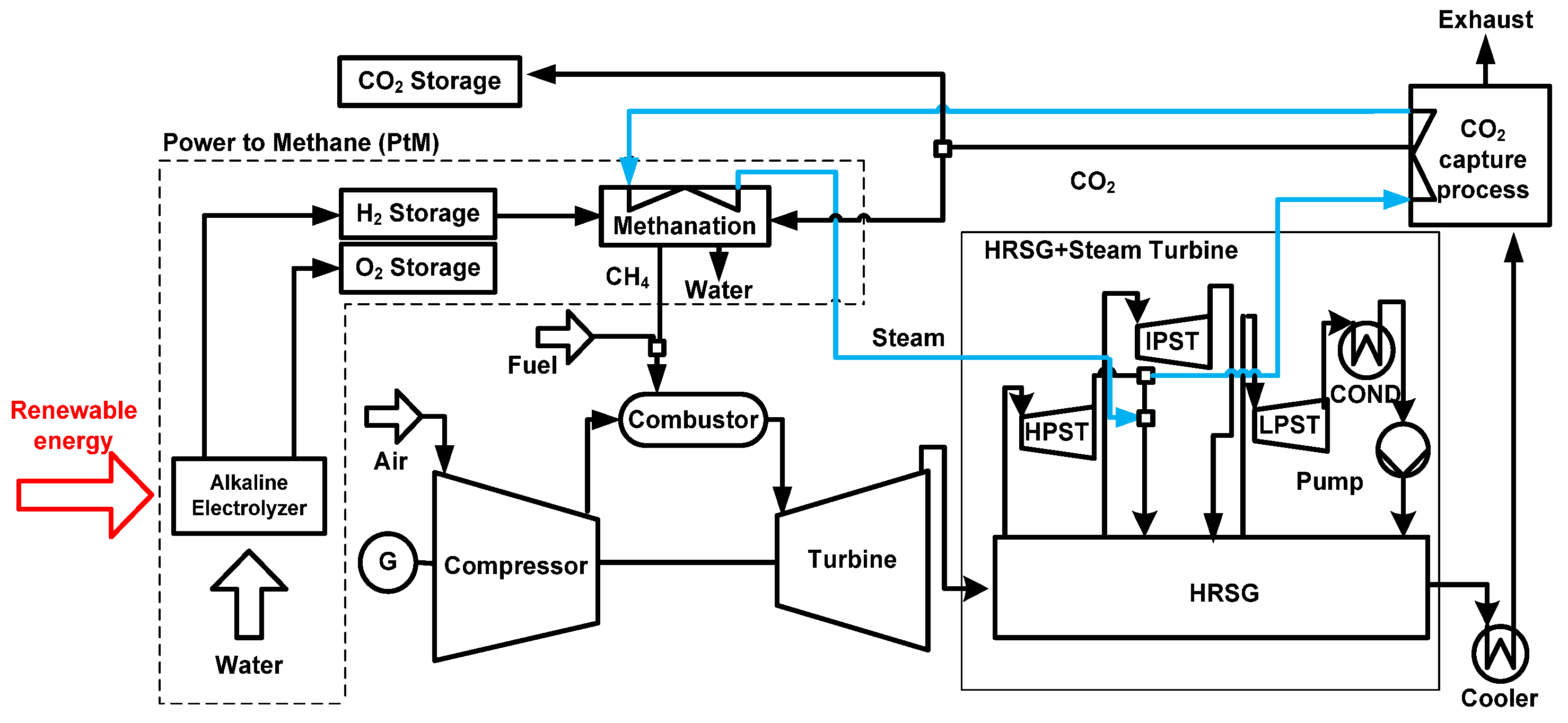
Layouts of the three systems are shown in Figure 1, Figure 2 and Figure 3. In Case 2, if the supply of is sufficient for operation, it operates using only ; otherwise, it uses a mixture of and NG. In Case 3, carbon dioxide is captured from the exhaust gas exiting the heat recovery steam generator (HRSG) by using the carbon capture process (CCP). This carbon dioxide and the hydrogen from the PtH process are used to generate methane-rich SNG in a methanation process (MP). A portion of the steam discharged from the high-pressure steam turbine (HPST) is used to provide the thermal energy needed for the CCP. Then, the steam enters the MP and absorbs the heat generated by the MP before finally being fed back to the bottom cycle. The produced SNG could be used as fuel for the GTCC.
2.2. System Modeling
2.2.1. Design Modeling of the GTCC
The GTCC simulation was performed using GateCycle [26]. The target GT was an M501GAC from Mitsubishi Heavy Industries. Its design specifications are available in the literature [25] and were used to model its design performance. The NG fuel is composed of 89% , 8.735% , 1.665% , 0.266% , 0.32% , and 0.008% by mole ratio, and its low heating value (LHV) is 49,426 kJ/kg. Unknown design parameters of the gas turbine were obtained through a simulation process that minimized the difference in the simulated and reference performance data. For example, the efficiencies of the turbine and compressor were determined to satisfy the inlet and outlet temperatures of the turbine and the total power output. The power output and efficiency of the GT were calculated using the following equations:
The simulated design performance was compared with reference data, and the results are shown in Table 2. All the major performance parameters such as the power, efficiency, and turbine exhaust temperature matched the reference data very well. The bottoming cycle was also modeled using GateCycle, and its design performance was calculated using the temperature, flow rate, and gas composition of the exhaust gas at the GT outlet. The major design values of the bottoming cycle are presented in Table 3.
The isentropic efficiency of each steam turbine was assumed to be 90%. Each pressure level of the HRSG included an economizer, an evaporator, and a superheater. The intermediate pressure level also included a reheater. All the heat exchangers were assumed to be of the counter flow type. The bottoming cycle power output was defined using Equation (3).
The net power and net efficiency of GTCC were defined using Equations (4) and (5), respectively.
The calculated design-point performance of the GTCC is also shown in Table 3. The results showed good agreement with the reference performance data available in the literature, indicating that the overall GTCC modeling was acceptable.
2.2.2. Off-Design Model of the GTCC
An off-design analysis is required to predict the performance changes resulting from the change in fuel, ambient conditions, and load. The efficiency, flow rate, and exhaust gas composition of the GT change with variations in the ambient temperature, electric load, and fuel composition. The changes in the GT operation affect the power output of the steam turbine, leading to changes in the performance of the GTCC.
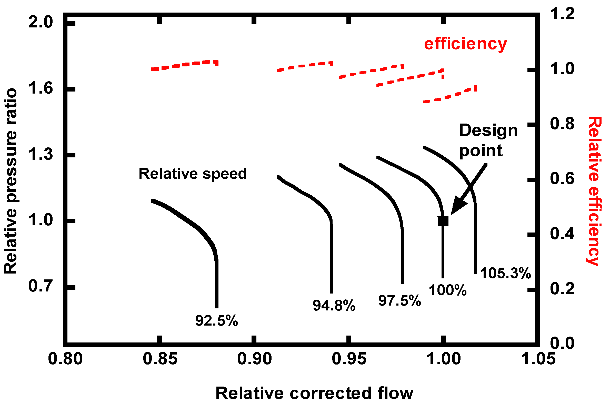
The off-design models of the turbomachinery parts, especially the compressor, are important for the simulation of the off-design behavior of the GT. For the compressor, the performance map of a compressor with a similar design point [26] was selected. The corrected performance map in Figure 4 was used in the simulation. This map is expressed in terms of the pressure ratio, efficiency, semi-dimensionless mass flow, and speed. The semi-dimensionless parameters are defined in the following equations. All four parameters are expressed in normalized forms relative to the design value.
Because the turbine generally operates under near-choking conditions, the following choking equation was applied to the off-design GT model [27].
The off-design operating point of the GT was determined by matching the compressor and turbine. There are two main methods of controlling the power output during off-design operation. One is adjusting the angle of the inlet guide vane (IGV) of the compressor and controlling the flow rate of the air injected into the GT, and the other is controlling the flow rate of the fuel. The IGV control improves the GTCC efficiency by keeping the TIT as high as possible during partial load operation [28]. However, because the TIT is very high, the IGV is usually controlled using the measured TET and a control curve.
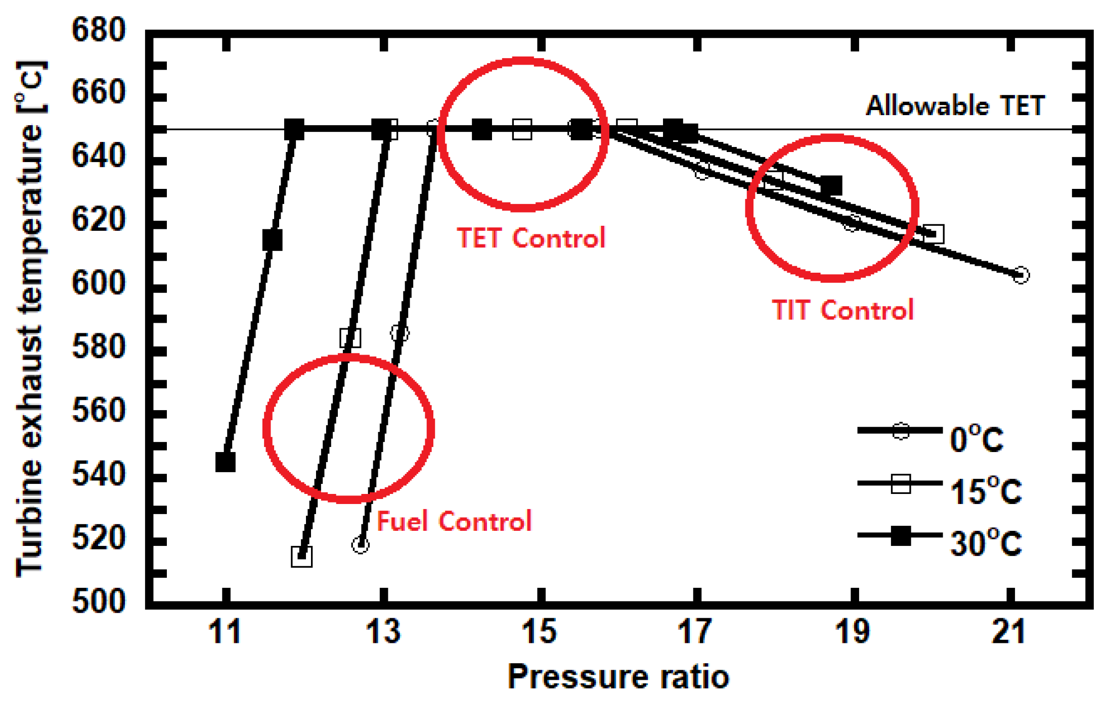
The TET control curve in Figure 5 was applied to the target GT. It was generated using the principle of the control logic of GTs [28] and the relation between the TET and pressure ratio obtained from the off-design simulation of the target GT. A higher pressure ratio means higher GT power output. The control curve consists of three parts. Firstly, when power is reduced from very high power conditions, the TIT is kept constant by closing the IGV and the TET increases. Once the TET limit is reached, it is maintained as constant. If the power is to be reduced further even after the IGV is fully closed, pure fuel control is adopted.
The effectiveness-NTU method was used for the off-design modeling of each heat exchanger section of the HRSG [29]. The modified Stodola equation was used for the steam turbine [26]. The steam turbine’s inlet pressure can be estimated based on the flow rate, outlet pressure, inlet temperature, and flow coefficient using the following equation:
where is the flow coefficient determined at the design point; and are the bowl pressure and bowl specific volume, respectively; r is the outlet pressure ratio; and r* is the critical pressure ratio.
2.2.3. Wind Power Data
A 4000-MW-scale offshore wind farm was assumed, and the individual wind power generators were assumed to be of the 5560-kW class. The location of the offshore wind farm is a southern province of Korea that is proposed as a site for wind farm construction. The surplus power of the wind farm was calculated using the annual wind speed data for the corresponding region [30]. The annual wind speed was measured at an altitude of 4 m and could be calibrated to the wind speed of the desired altitude using Equation (10).
The power generated by a wind power generator was calculated using Equation (11):
where r is the radius of the turbine blades, ρ is the density, and η is the mechanical efficiency, which includes the generator. The exponent 0.1 in Equation (10) is the wind shear exponent determined by the ground conditions (open water).
The height of the hub of the wind power generator was assumed to be 100 m, and the blade length was 68 m. The wind speed (H) at 100 m (Z) was obtained by applying Equation (10) to the wind speed () measured at an altitude of 4 m () [31]. Then, H was inserted into Equation (11) to estimate the power output (kW). The design specifications used for the wind power calculation are summarized in Table 4 [32].
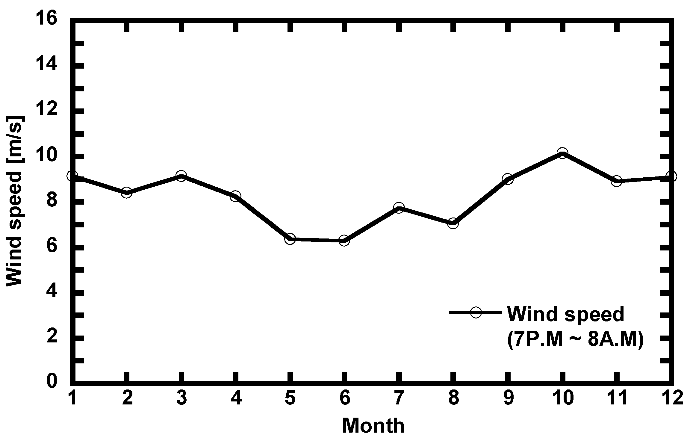
In general, the power demand is high during the day, and surplus power occurs at night [33]. This tendency clearly appears in another study [34] as well. Therefore, it was assumed that the surplus power generated from the offshore wind farm was used for production rather than supplied to the power grid in the 13 h period (7 p.m. to 8 a.m.) when the power demand was low. The average wind speed for a 4-year period in the target region [30] was used for the wind speed of the offshore wind farm between 7 p.m. and 8 a.m. The wind power data are summarized in Table 5. The variation in the monthly average wind speed is shown in Figure 6.
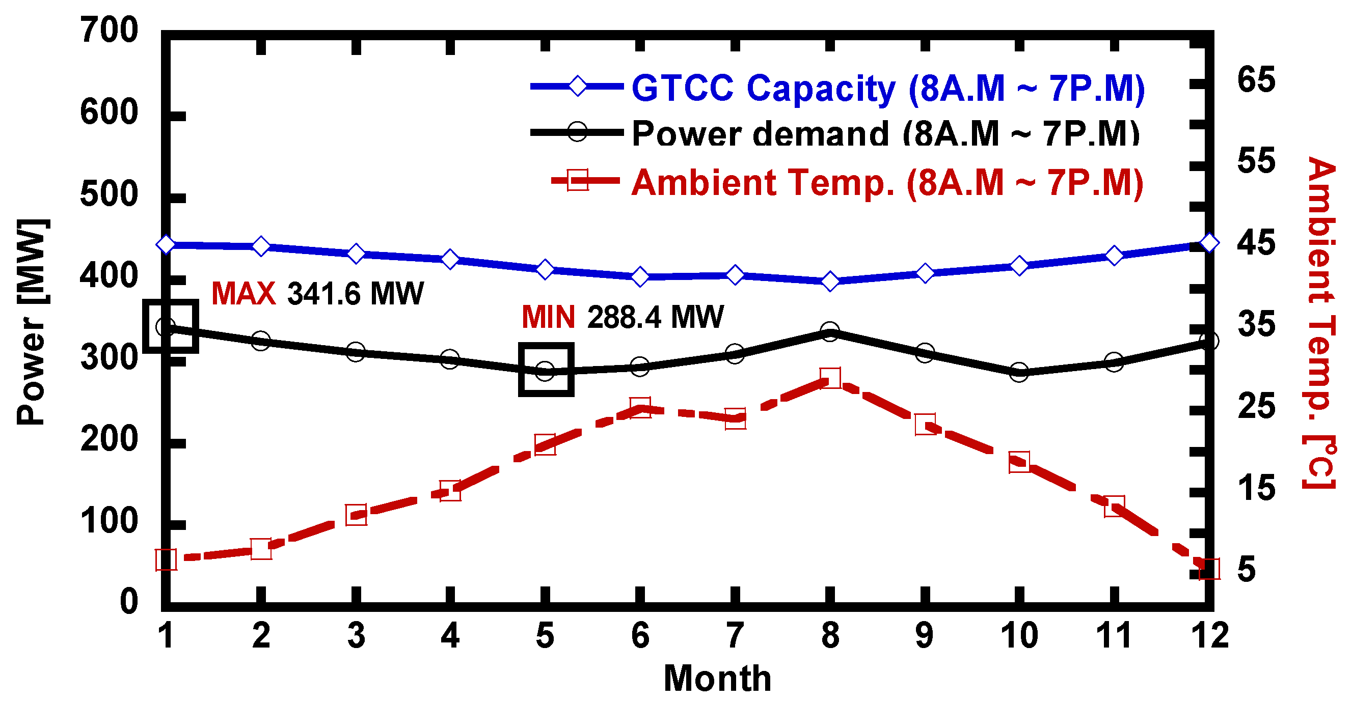
2.2.4. Electricity Demand and Ambient Temperature Data
The GTCC operating time was assumed to be 11 h during daytime when the electricity demand is high (8 a.m. to 7 p.m.). The actual electricity demand pattern and ambient temperature of the region where the power plant was located were taken into account when determining the daytime operational performance. The GTCC plant was assumed to be located in the southern coastal area of South Korea adjacent to an offshore wind farm. The average ambient temperature of the corresponding area was also obtained from meteorological data [30].
The annual variation in the power demand was generated based on the pattern of the national power demand of South Korea [35]. Both the ambient temperature and power demand data were 4-year averages. The variations in the ambient temperature and power demand that had to be addressed by the GTCC power plant are presented in Figure 7. The power demand of January, when the demand is the highest, was assumed to be 341.6 MW, which is 80% of the design load of the GTCC.
2.2.5. PtG Process
The amount of hydrogen that can be produced per megawatt at the current level of PtG technology can be found in the literature [24]. Therefore, rather than performing detailed modeling of the PtG process, was assumed to be produced by a PtG water electrolysis process with a specific power consumption of 20.833 kg/MWh [24]. The power available for the electrolysis process (the net surplus power) is the net power output, which is the difference between the total produced power () and the power consumption used for storing hydrogen (). Hence, the hydrogen production using the surplus power can be calculated using the following equation.
The PtG capacity is assumed to be 1900 MW. Although the capacity of the offshore wind farm is 4000 MW, the actual average wind speed is 8.3 m/s, which does not correspond with the rated wind speed of the wind power generator of 10 m/s. Accordingly, it was predicted that the generated monthly average surplus power would not exceed 1900 MW.
2.2.6. CCP
Basically, three methods are available for carbon capture: post-combustion, pre-combustion, and oxy-combustion capture. Post-combustion capture is the most mature technology and requires the least modification to existing power plants [36]. Several capture processes are available for post-combustion capture, but the MEA process was adopted because it is the most mature and common.
Post-combustion capture is a relatively mature technology, and performance data such as its specific energy consumption are also relatively well known. At a capture rate of 90%, the specific thermal energy demand was assumed to be 3.85 [37]. Accordingly, the consumed electric power and thermal energy were determined as follows based on the rate of collected through the CCP (kg/s):
In CCP, power is consumed by pumps and compressors. In the MEA process, an internal pump is used, but the power consumption of the pump is very small compared to the overall system power. Therefore, the power consumption of the pump was simplified to 2.7% of the power consumption of the CCP compressor. To process at 1.02 bar collected using the MEA process into high-purity , the compressor compresses it to 30 bar and transfers it to a separator. During this process, the compressor’s efficiency was 90%, and the consumed power was calculated using the same performance simulation program that was used for the GTCC [26]. The design values of this amine-scrubbing technique are presented in Table 6. The power consumed in the CCP was calculated using the following equation:
2.2.7. Methanation Process
MP is also widely known, so instead of performing a detailed simulation, the literature data for this process were used. The TREMPTM process was employed, which uses the Sabatier reaction operating at high pressure and high temperature using nickel-based catalysts [38]. The SNG produced through the MP was composed of 98% and 2% + Ar by mole ratio, and the LHV of the SNG was 48,306 kJ/kg. The Wobbe index of the syngas is in the range of that of the NG, thus confirming that it is interchangeable with NG (i.e., it can be used in an existing GT without revising the combustor).
In the MP, the energy used at the recycling compressor to increase the temperature of the TREMPTM process reactor was calculated as the consumed power. A specific power consumption of 108 kJ/kg was adopted for the recycle compressor based on a previous study [21]. The thermal energy generated from the MP was determined by the amount of hydrogen used [24]. As a result, the rates of power consumption and thermal energy generation were calculated by the following expressions:
Considering the SNG output and LHV produced during the methanization process, the MP was assumed to be on the scale of 650 MW.
2.3. Operation Strategy
Three GTCC operation strategies were compared. Case 1 is an existing GTCC model that uses NG as a fuel. Case 2 uses an existing GTCC model similar to Case 1, except that and NG are used as fuels. In Case 3, the present in the exhaust gas of the GTCC is captured using the CCP. If the supply of decreases, the heat generated by the MP also decreases. In this case, it is not possible to obtain the energy required to operate the bottoming cycle. Thus, if the supply is not sufficient, it reduces the capture rate in the CCP, thereby reducing the energy consumption of the CCP.
The GTCC in each case used the DSS method during the 11 h daytime period. During the daytime, the power generated from the offshore wind farm and GTCC is supplied to the power grid. During the 13 h in which the power demand is low and the GTCC does not operate, the power generated from the offshore wind farm is not supplied to the power grid and is instead used to produce through the PtG process.
The basic equations to calculate the GTCC performance are summarized in Equations (1)–(5) in Section 2.2.1. However, some revisions in the calculations were required in Cases 2 and 3 because they used and SNG along with NG as fuels. Furthermore, additional power consumption was needed for the SNG production in Case 3. The revised equations are as follows:
In Case 2, and NG were used as fuel, whereas in Case 3, SNG and NG were used. The energy of the injected fuel was calculated based on the mixing ratio of the two fuels. The ambient temperature, wind speed data, and power demand pattern were reflected in the off-design analysis of the actual operating cycle. The partial load operation of the GTCC used the IGV control method in conjunction with fuel flow control. The amount of available changed with the wind speed. If hydrogen production was sufficient, Case 2 could operate using only , whereas in Case 3, the mixing ratio of SNG increased. Otherwise, the use of NG increased in both cases.
2.4. Economic Analysis
The addition of PtG, CCP, and MP equipment naturally increases the installation cost and the operations and maintenance (O&M) cost, while the reduced NG usage and reduced CO2 emissions act as benefits. The purpose of the economic analysis was to estimate the economic benefits of Cases 2 and 3 over Case 1 and to evaluate which one of them is economically superior. Therefore, the economic feasibility of the additional investment (the incremental capital expenditure (CAPEX)) of Cases 2 and 3 over the normal GTCC was evaluated.
In Cases 2 and 3, various additional facilities are required, including the hydrogen production infrastructure, which requires additional investment. According to a preliminary evaluation, the current market prices of the additional facilities such as the PtG process are too high to guarantee a feasible payback of the investment. Therefore, we used predicted future price data in the year 2030, when the green hydrogen production and use is expected to be more technically and commercially mature.
The data used for the economic analysis are shown in Table 7. The GT and GTCC prices for the year 2030 were calculated based on the assumption that the rate of price change (3.94%) over the last five years will remain constant [25,39]. The increase in the GT cost () due to its revision to accommodate hydrogen combustion was considered for the GT of Case 2. In the case of the O&M cost, existing data were used [40,41], and the annual operation time was set to 4015 h/year in accordance with the DSS power generation method.
The reference capital cost of the PtG system in 2020 was set as 650 USD/kW [11]. The PtG cost is expected to rapidly decrease following technological development. The cost is predicted to decrease to 130 USD/kW by 2050 [11]. Assuming that this price will change linearly, the PtG price for 2030 was set to be 27% lower than that for 2020. The capital cost of CCP was set to be 70% of the GTCC installation cost after referring to a previous economic analysis [42]. A value of 75.3 USD/kW was used as the MP equipment cost for 2030 based on a price estimation method [43].
The O&M cost of PtG was assumed to be 4% of the installation cost [41]. Also, the water price for electrolysis was considered [44]. The O&M cost of the CCP was set to be 12% of the installation cost [42], and that of the MP system was assumed to be 10% of the installation cost [45]. The engineering cost of the PtG, CCP, and MP was assumed to be 28% of the capital cost of each component [41]. The project period of the three cases was set as 30 years.
The NG price in Korea as of 2020 is USD 43.3/MWh. Referring to the latest predicted trend of the NG price increase [48], the NG price in 2030 was set as 1.5 times higher than that in 2020. The Korea tax of 2030 was determined in accordance with the “Tax Policy and Climate Change (2021)” [47]. In order to achieve the Paris Agreement target’s nationally sensitive contributions (NDCs) by 2030, South Korea must raise the CO2 tax by more than USD75/tCO2 from 2020 prices. Therefore, the CO2 tax in 2030 was calculated to be 108 USD/tCO2 (up USD 75 from 33 USD/tCO2 in 2020).
All the cost data from various sources were standardized to USD using the reference exchange rates of 21 March 2021: 0.00088 USD/KRW and 1.2 USD/EURO. For example, the water price was converted from KRW to USD and the MP and hydrogen prices were converted from EURO to USD. We intended to estimate the incremental benefit of the additional investment in Cases 2 and 3 in comparison to Case 1, so the GTCC’s installation, operation, and electricity sales revenues were excluded since they were the same in all three cases.
The CAPEX of Case 2 consists of the PtG equipment and engineering cost and the GT revision cost, while that of Case 3 includes the equipment and engineering costs of the PtG, CCP, and MP. In the following equations, W denotes the capacity of each plant or process ( = 1900 , = 283 , = 427 and = 650 ).
The annual O&M costs of Cases 2 and 3 were calculated as constant ratios of the CAPEX of the additional components such as the PtG, CCP, and MP.
The operational expenditures (OPEXs) of Cases 2 and 3 should be reduced compared to Case 1 to guarantee a payback. In other words, the OPEX savings are the economic benefit of Cases 2 and 3 that can cancel out the investment (i.e., the CAPEX). The source of OPEX savings is cost avoidance due to huge reductions in NG purchases and tax. The increase in the O&M cost of the added components and increased demand for water have negative effects on OPEX savings. The annual OPEX savings were calculated using the following equation:
Equation (24) was used to calculate the payback period (PB) using the net present value (NPV) method. The NPV is the present value converted from the total profit after a certain period considering the discount rate. The PB is the point in time when the total profit NPV turns from negative to zero. The discount rate was assumed to be 0.05 (5%).
The comparison of the PBs of Cases 2 and 3 indicates the relative economic advantages of one over the other.
3. Results and Discussion
3.1. Performance Analysis
3.1.1. Influence of Hydrogen Co-Firing Ratio
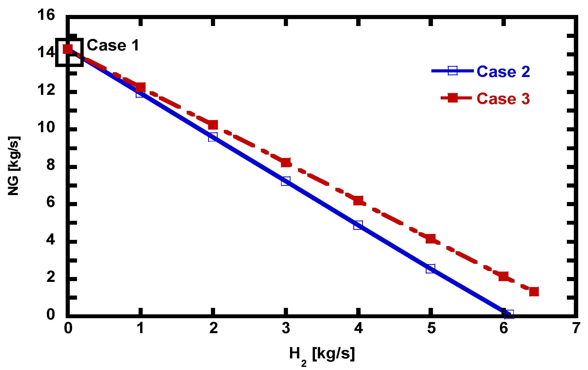
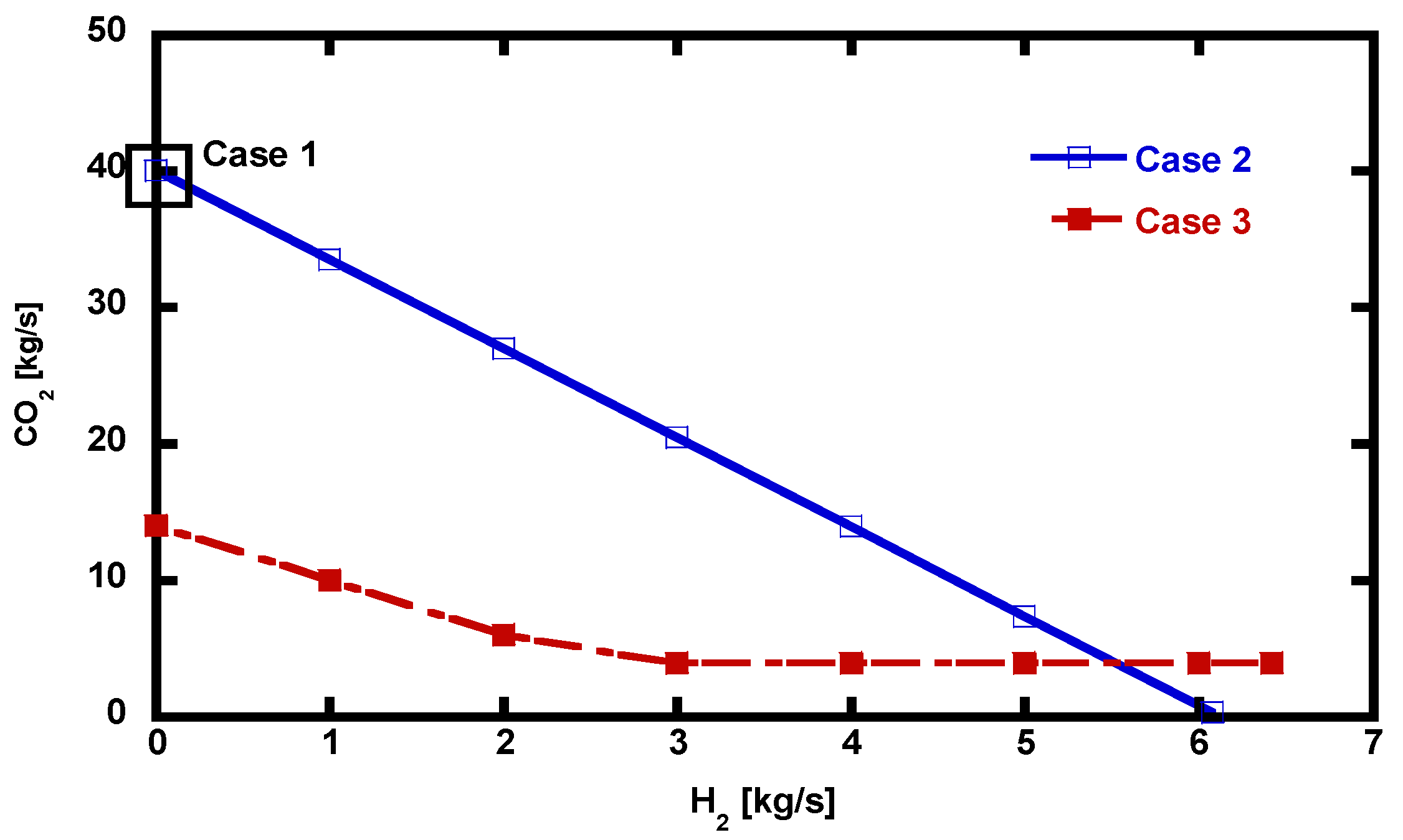
As a first step of our analysis, we investigated the fundamental impact of increasing the hydrogen mixing ratio in the fuel on the performance and emissions characteristics of Cases 2 and 3. The performance of the two cases was comparatively analyzed by changing usage. Performance comparisons were conducted under the design conditions presented in Table 2 for each case (TIT, PR, and temperature conditions). The changes in the NG usage and emissions of Cases 2 and 3 were compared, and the results are shown in Figure 8 and Figure 9, respectively.
In Case 2, the supply varied from 0 kg/s to 6.08 kg/s (0 to 100% mole fraction). As the supply increased, the emissions and NG usage linearly decreased. When sufficient was supplied, 6.08 kg/s of could completely replace 14.27 kg/s of NG, and the emissions decreased from 39.75 kg/s to 0 kg/s. With increasing usage, the combustion gas contained more , which had higher specific heat than other components. As a result, the power output and efficiency of the turbine increased compared to Case 1. When the GT was driven by pure , Case 2 showed 4.9% higher power output and 0.9%p higher efficiency than Case 1. These results are shown in Table 8.
Similar to Case 2, the mixing ratio of Case 3 also affected the emissions and NG usage. The maximum supply that could react with all captured was 6.42 kg/s. In these operating conditions, 90% of the emitted from the GTCC could be captured, and the NG usage could be reduced by 90.7% from 14.27 kg/s in Case 1 to 1.33 kg/s.
The NG usage of Case 2 was always lower than that of Case 3, as shown in Figure 8. If enough was supplied in Case 2, hydrogen could completely replace NG. On the other hand, NG supply was still required in Case 3, even in the maximum supply conditions, because the in the exhaust gas could not be completely converted to the SNG due to the limitation of the carbon capture rate of the CCP. The minimum NG supply was predicted to be 1.33 kg/s.
The emissions of Case 3 were lower than in Case 2 in a wide range of supply ratios, as shown in Figure 9. This happened because unlike Case 3, which captured from the exhaust gas through the CCP, Case 2 did not have a separate removal measure. Thus, an increase in NG usage led to an increase in emissions. In the case where was not provided, the carbon capture rate was further decreased to 65% at the CCP. However, if the hydrogen supply was sufficient (i.e., the supply ratio was very high), could completely replace the NG in Case 2, and the emissions were zero, which was lower than in Case 3.
3.1.2. Performance Comparison for Annual Operation
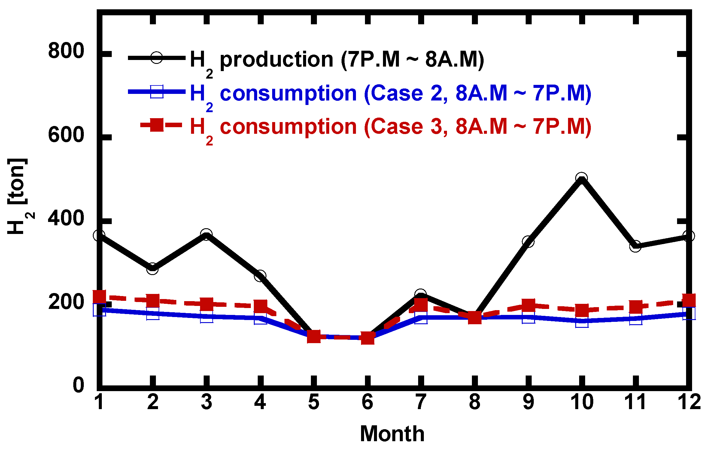
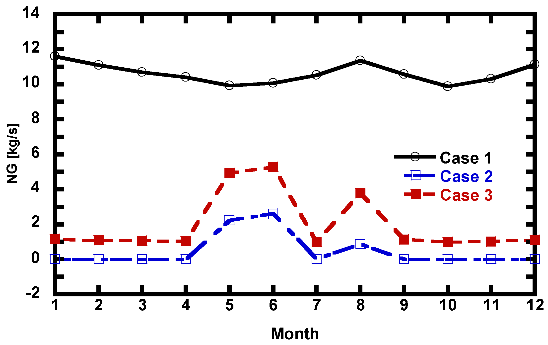
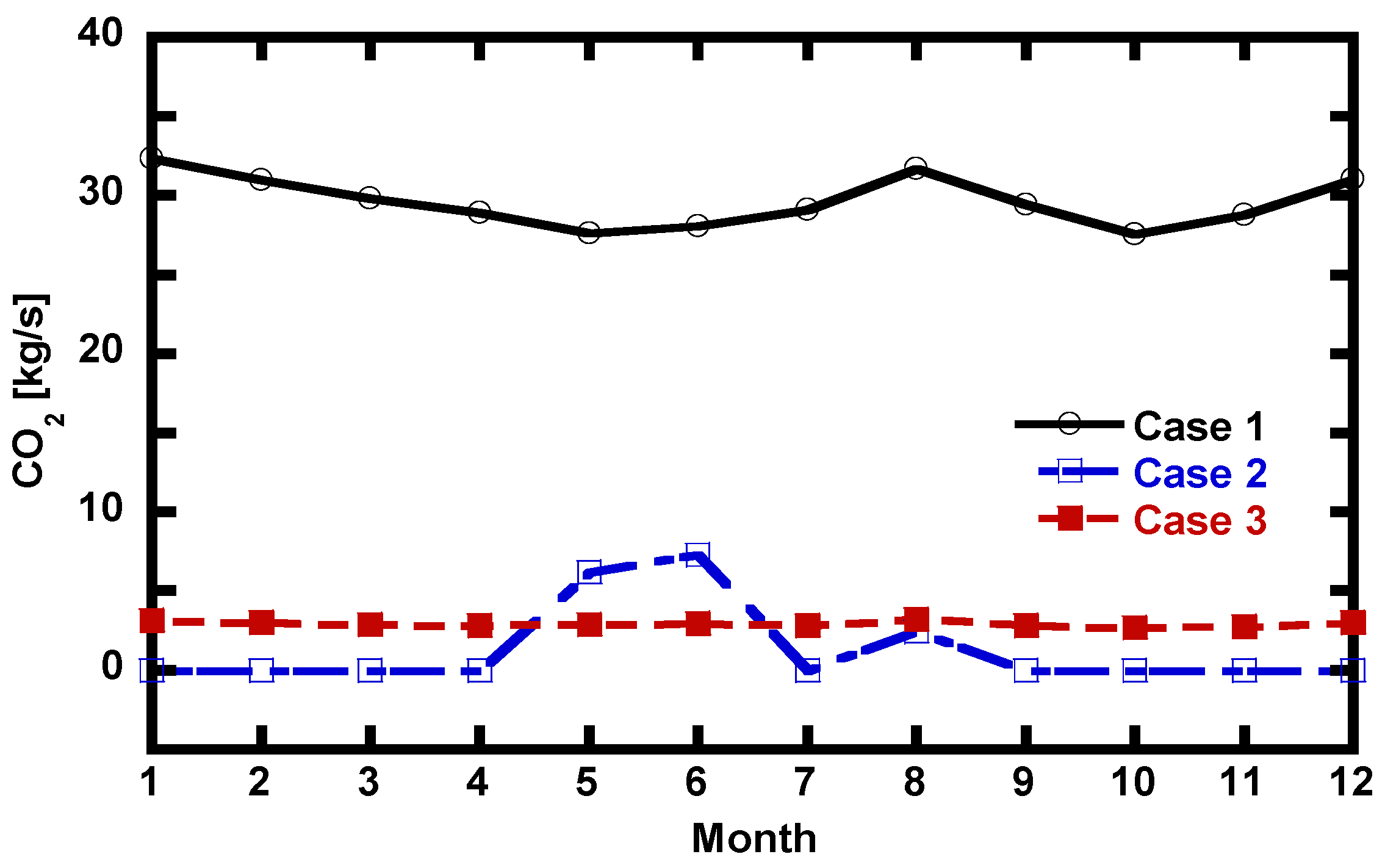
The annual performance was predicted using the variation in the power demand of the GTCC and ambient temperature in Figure 7 and the variation in surplus wind power production calculated by the wind speed data in Figure 6. A higher wind speed at night made it possible to produce a greater amount of surplus power, resulting in an increase in the amount of available during the day. Because the monthly average wind speed varied, the amount of supplied to the GTCC was different in each month. The usage, NG usage, and emissions of each case are presented in Figure 10, Figure 11 and Figure 12, respectively.
was produced and stored using the surplus power generated for 13 h in the 4000-MW-scale offshore wind farm and was used during the 11 h of daytime when the power demand was high. The surplus wind power decreased in May, June, and August when the average wind speed at night was relatively low (see Figure 6). This resulted in relatively low production of in these three months (see Figure 10).
In Case 2, NG had to be supplied to the GTCC in the three months of May, June, and August (see Figure 11) when the power demand could not be satisfied using only the . The GTCC was operated using only in the other nine months when sufficient was supplied. In Case 3, a change in the supply also led to a change in the SNG production, which affected the NG usage. Therefore, the SNG production decreased in May, June, and August, and the NG supply pattern was similar to that of Case 2. Thus, unlike Case 2, a certain amount of NG was required for the GTCC operation, even if the supply was sufficient (Figure 11).
The average NG usage of Case 2 in May, June, and August was 81.7% lower than in Case 1 and 59.0% lower than in Case 3. The annual average NG usage of Case 2 was 0.48 kg/s, which was 98.4% lower than in Case 1 and 76.0% lower than in Case 3. The emissions were proportional to the NG usage in Cases 1 and 2 because the produced in the combustor was exhausted to the power plant stack (see Figure 12). However, in Case 3, 90% of the from the GTCC was captured, and only 10% was produced in all seasons. Therefore, the emissions of Case 3 were almost constant throughout the year. In Case 2, the emissions were zero in the nine months when pure hydrogen was used as fuel, while it emitted about 50% more than in Case 3 in the three months of May, June, and August when NG had to be used. Nevertheless, the annual average emissions of Case 2 were 54.6% lower than that of Case 3. The average reduction in Case 2 from Case 1 was 95.5%.
3.2. Economic Analysis
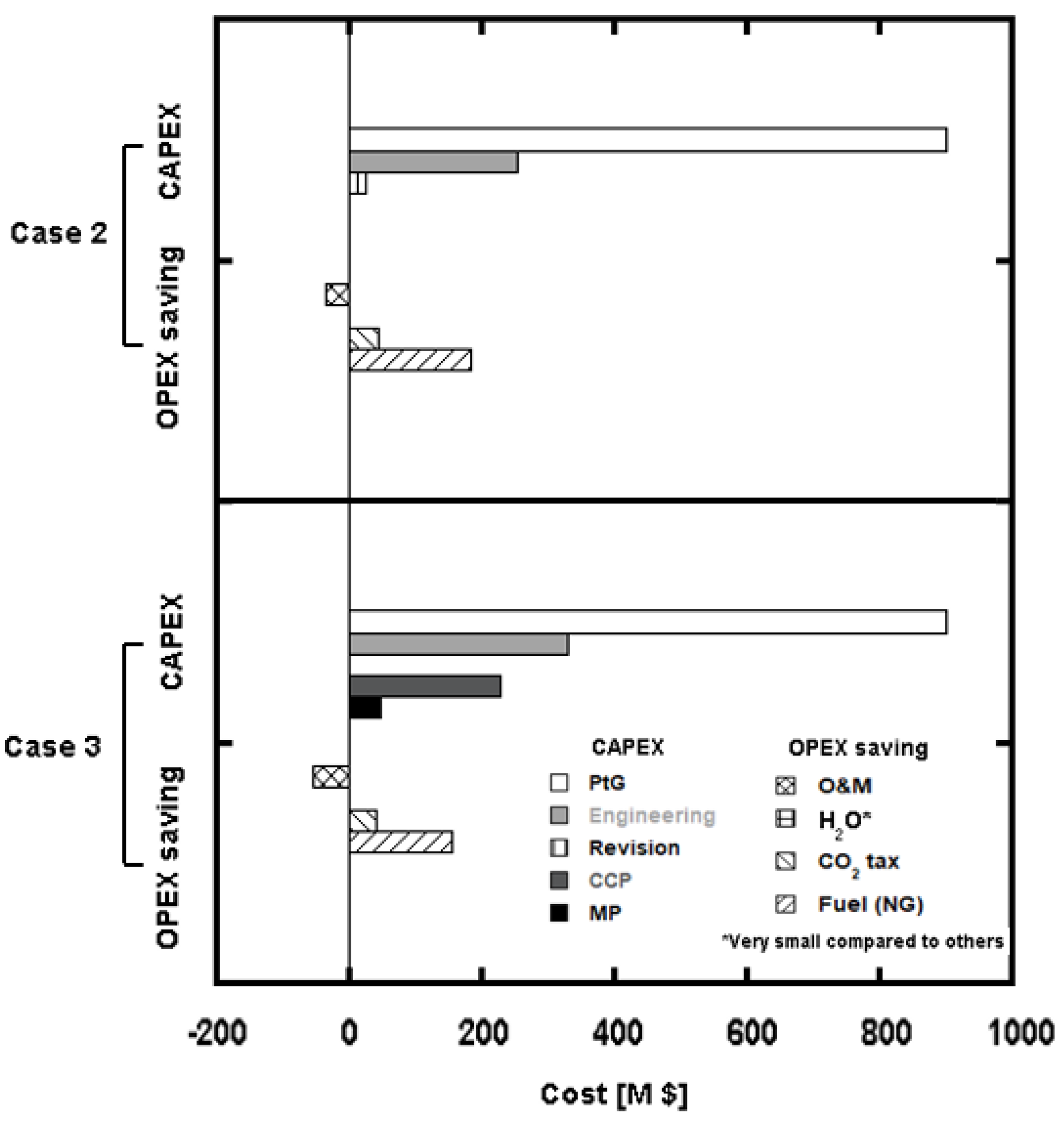
Table 9 summarizes the results of the economic analysis, and Figure 13 presents the breakdowns of the CAPEX and OPEX savings for each case. Considerable CAPEX should be invested in Cases 2 and 3 through the installation of various components required for the PtG, CCP, and MP systems in comparison to the conventional power plant of Case 1. In Case 2, the CAPEX due to the initial investment was calculated to be USD 1.18 billion. It mostly comprised the PtG cost (76.5%), while the GT revision cost and engineering cost were 2.1% and 21.4% respectively. In Case 3, the CAPEX was USD 1.51 billion, which was 28% higher than in Case 2 due to the addition of the CCP and MP.
The addition of components in Cases 2 and 3 led to an increase in the O&M costs. The annual O&M cost of Case 2 was USD 36.1 million higher than that of Case 1, and that of Case 3 was USD 68.5 million higher than that of Case 1. Such increases in the CAPEX and O&M costs could be recovered through the OPEX saving.
Because Cases 2 and 3 were supplied with fuel using generated from surplus power, the savings of NG purchases would be huge. In Case 2, was directly used, while in Case 3, was captured through the CCP, and a portion of the used NG was replaced with SNG. Through this operational method, less was produced in Cases 2 and 3, enabling a reduction in the tax as well. Such an OPEX reduction contributed to recovering the increased initial investment costs resulting from the CAPEX increase. The annual OPEX savings of Case 2 were calculated to be USD 138.8 million. The OPEX savings of Case 3 was even lower than Case 2 (USD 84.6 million).
The payback periods for the CPAEX were predicted to be 11.4 and 45.9 years for Cases 2 and 3, respectively. The payback period of Case 2 was almost a quarter that of Case 3. The shorter payback period of Case 2 was attributed to two factors: its CAPEX was lower, but its OPEX savings were higher. Therefore, the direct combustion of hydrogen (Case 2) is economically more beneficial than the conversion of hydrogen to syngas (Case 3).
It is also interesting that the payback periods of Case 2 were sufficiently less than the normal plant lifetime, which is usually more than 20 years. In particular, the relatively short payback period of Case 2 is encouraging. Of course, it should be noted that the current result was drawn from a future cost scenario (2030). When we used the current costs based on the year 2020, the CAPEX was more than 25% higher, and the OPEX savings were less than 40% of those in Table 9. This leads to a very long payback period of over one hundred years, which means that the investment is not economically feasible. Another point is that the economics also depend heavily on the NG price because the savings of NG consumption are the majority of the OPEX savings. Accordingly, the payback period highly depends on the NG price.
The current analysis was based on the 2021 version of the NG price forecast [47], which predicts an increase of 1.5 times from 2020 to 2030. This assumption is NG price scenario 1. However, according to the 2020 version of the same report [49], the increase was predicted to be 2.1 times. This indicates that there is a high uncertainty in predicting the NG price. The results for the 2020 price data are summarized in Table 10. According to this assumption (NG price scenario 2), the payback periods of Case 2 and 3 are 7.7 and 15.1 years, which are dramatically reduced from the current results of 11.4 and 45.9 years, respectively. This comparison indicates two things: the importance of the NG price and the fact that Case 2 would be more economical regardless of the NG price.
The important findings from the current economic analysis are as follows. Firstly, the direct combustion of hydrogen in the GT would be an economically better option if the expected technology development is achieved as projected. Secondly, the CAPEX reduction is crucial, and the two proposed schemes, especially direct combustion, would be economically viable if the current predicted 2030 cost data are realized.
4. Conclusions
This study analyzed the performance and economic feasibility of a GTCC plant combined with hydrogen production using surplus power from an offshore wind farm. The research focus was to identify the potential of emissions reduction and economic feasibility of the GTCC plant integrated with either a PtH or PtM system in comparison to a conventional NG-fired GTCC model. Annual variations in the operations of the wind farm and GTCC were taken into account, and economic factors expected in 2030 were used. The results and conclusion are summarized as follows.
- It was predicted that the annual CO2 emissions would be 95.5% lower in the GTCC-PtH plant and 89.7% lower in the GTCC-PtM plant in comparison to the conventional NG-fired GTCC plant. In the months when H2 is sufficiently supplied, the GTCC-PtH plant using hydrogen directly as fuel for the GTCC emits less CO2 than the GTCC-PtM plant that removes CO2 after combustion. Based on the results of the annual CO2 emissions and fuel usage, the environmental performance of direct hydrogen combustion option (i.e., the GTCC-PtH plant) is expected to be better.
- The GTCC-PtH plant models seem to provide reasonable economics when assuming the cost scenario of 2030, but they would not provide viable economics when using current cost data. The CAPEX is lower and the OPEX savings is higher in the GTCC-PtH plant, which make its payback period much shorter in comparison to the GTCC-PtM plant.
- As the share of renewable energy further increases, the need for technologies that could secure power grid stabilization and resolve the problems of surplus power generation is also rapidly escalating. The significance of this study is that it suggests a possible solution that integrates a GTCC plant with PtG technology and has provided detailed performance and economic analyses for two viable technical options.
Author Contributions
Conceptualization, M.-J.P., T.-S.K., methodology, M.-J.P., S.-W.M., software, M.-J.P., S.-W.M., formal analysis, M.-J.P., investigation, M.-J.P., S.-W.M., resources, T.-S.K., data curation, M.-J.P., writing—original draft, M.-J.P., writing—review and editing, M.-J.P., T.-S.K., supervision, T.-S.K., project administration, T.-S.K., and funding acquisition, T.-S.K. All authors have read and agreed to the published version of the manuscript.
Funding
This work was supported by the Korean Institute of Energy Technology Evaluation and Planning (KETEP) grant funded by the Korean government (MOTIE) (No. 20206710100030, Development of Eco-friendly GT Combustor for 300 MWe-class High-efficiency Power Generation with 50% Hydrogen Co-firing).
Institutional Review Board Statement
Not applicable.
Informed Consent Statement
Not applicable.
Conflicts of Interest
The authors declare no conflict of interest.
Nomenclature
| A | Area (m2) |
| C | Cost (USD/kg) |
| CP | Constant pressure specific heat (kJ/kg·K) |
| Cq | Flow coefficient |
| E | Engineering cost (USD/kW) |
| H | Corrected wind speed (m/s) |
| Ha | Measured wind speed (m/s) |
| h | Enthalpy (kJ/kg) |
| i | Discount rate |
| Mass flow rate (kg/s) | |
| N | Revolutions per minute |
| P | Pressure (kPa) |
| R | Gas constant (kJ/kg·K) |
| T | Temperature (K) |
| t | Time (hour) |
| U | Unit capital cost (USD/kW) |
| W | , ) |
| Power (MW) | |
| Y | Gas price (USD/MW, USD/kg) |
| Z | Corrected altitude (m) |
| Za | Measured altitude (m) |
| γ | Specific heat ratio |
| η | Efficiency |
| v | Specific volume (m3/kg) |
Abbreviations
| CCP | Carbon capture process |
| CAPEX | Capital expenditure |
| DSS | Daily start and stop |
| ESS | Energy Storage System |
| GT | Gas turbine |
| GTCC | Gas turbine combined cycle |
| HP | High pressure |
| IGV | Inlet guide vane |
| IP | Intermediate pressure |
| LP | Low pressure |
| MEA | Monoethanolamine |
| MP | Methanation process |
| NG | Natural gas |
| O&M | Operations and Maintenance |
| OPEX | Operational expenditure |
| PtG | Power to gas |
| PtH | Power to hydrogen |
| PtM | Power to methane |
| TIT | Turbine inlet temperature |
| TET | Turbine exhaust temperature |
| SNG | Synthetic natural gas |
| ST | Steam turbine |
Subscripts
| Comp | Compressor |
| b | Bowl |
| d | Design |
| el | Electric |
| g | Gas |
| gen | Generator |
| m | Mass flow |
| mech | Mechanical |
| s | Steam |
| Turb | Turbine |
| th | Thermal |
References
- Deng, X.; Lv, T. Power system planning with increasing variable renewable energy: A review of optimization models. J. Clean. Prod. 2020, 246, 118962. [Google Scholar] [CrossRef]
- Ghassemi, A. Wind Energy, Renewable Energy and the Environment, 3rd ed.; CRC Press: Boca Raton, FL, USA, 2019. [Google Scholar]
- Ferroukhi, R.; Hawila, D.; Khalid, A. Renewable Energy Benefits Leveraging Local Capacity for Solar PV; IRENA: Masdar City, United Arab Emirates, 2017. [Google Scholar]
- Renewables 2020 Analysis and Forecast to 2025. Available online: https://iea.blob.core.windows.net/assets/1a24f1fe-c971-4c25-964a-57d0f31eb97b/Renewables_2020-PDF.pdf (accessed on 1 November 2021).
- Bird, L.; Milligan, M.; Lew, D. Integrating Variable Renewable Energy: Challenges and Solutions; Prepared under Task No. WE11.0820; National Renewable Energy Laboratory: Golden, CO, USA, 2013.
- Čonka, Z.; Kolcun, M.; Morva, G. Impact of Renewable Energy Sources on Power System Stability. Power Electr. Eng. 2014, 32, 25–28. [Google Scholar] [CrossRef] [Green Version]
- Martin, R.; Donohue, J. The 7FA Gas Turbine “A Classic Reimagined”; GE Energy: Greenville, SC, USA, 2009. [Google Scholar]
- World Energy Outlook. Available online: https://iea.blob.core.windows.net/assets/a72d8abf-de08-4385-8711-b8a062d6124a/WEO2020.pdf (accessed on 1 November 2021).
- Aneke, M.; Wang, M. Energy storage technologies and real life applications—A state of the art review. Appl. Energy 2016, 179, 350–377. [Google Scholar] [CrossRef] [Green Version]
- Beaudin, M.; Zareipour, H.; Schellenberglabe, A.; Rosehart, W. Energy storage for mitigating the variability of renewable electricity sources: An updated review. Energy Sustain. Dev. 2010, 14, 302–314. [Google Scholar] [CrossRef]
- Taibi, E.; Blanco, H.; Miranda, R.; Carmo, M.; Gielen, D.; Roesch, R. Green Hydrogen Cost Reduction, Scaling up Electrolysers to Meet the 1.5 °C Climate Goal; IRENA: Masdar City, United Arab Emirates, 2020. [Google Scholar]
- Jones, R.; Goldmeer, J.; Monetti, B. Addressing Gas Turbine Fuel Flexibility; GE Energy: Boston, MA, USA, 2011. [Google Scholar]
- Hydrogen Gas Turbines, The Path towards a Zero-Carbon Gas Turbine. Available online: https://etn.global/wp-content/uploads/2020/01/ETN-Hydrogen-Gas-Turbines-report.pdfydrogen-Gas-Turbines-report.pdf (accessed on 1 November 2021).
- Eveloy, V.; Gebreegziabher, T. A Review of Projected Power-to-Gas Deployment Scenarios. Energies 2018, 11, 1824. [Google Scholar] [CrossRef] [Green Version]
- POWERing the World with Gas Power Systems; GE Power: Boston, MA, USA, 2016.
- Marra, J. Siemens Perspective on Future Hydrogen Fuel; Siemens: Munich, Germany, 2019. [Google Scholar]
- Parra, D.; Zhang, X.; Bauer, C.; Patel, M.K. An integrated techno-economic and life cycle environmental assessment of power-to-gas systems. Appl. Energy 2017, 193, 440–454. [Google Scholar]
- Stambasky, J. Power to Methane, an Integral Part of Biomethane Industry; European Biogas Association: Ghent, Belgium, 2017. [Google Scholar]
- O’Shea, R.; Wall, D.M.; McDonagh, S.J.; Murphy, D. The potential of power to gas to provide green gas utilising existing CO2 sources from industries, distilleries and wastewater treatment facilities. Renew. Energy 2017, 114, 1090–1100. [Google Scholar] [CrossRef]
- Safari, F.; Dincer, I. Assessment and optimization of an integrated wind power system for hydrogen and methane production. Energy Convers. Manag. 2018, 177, 693–703. [Google Scholar] [CrossRef]
- Won, D.H.; Kim, M.J.; Lee, J.H.; Kim, T.S. Performance characteristics of an integrated power generation system combining gas turbine combined cycle, carbon capture and methanation. J. Mech. Sci. Technol. 2020, 34, 4333–4344. [Google Scholar] [CrossRef]
- Yang, J.; Cheng, Y.; Xia, Q. Modeling the Operation Mechanism of Combined P2G and Gas-Fired Plant with CO2 Recycling. IEEE Trans. Smart Grid 2019, 10, 1111–1121. [Google Scholar] [CrossRef]
- Liu, J.; Sun, W.; Harrison, G.P. The economic and environmental impact of power to hydrogen/power to methane facilities on hybrid power-natural gas energy systems. Int. J. Hydrogen Energy 2020, 45, 20200–20209. [Google Scholar] [CrossRef]
- Reiter, G.; Lindorfer, J. Global warming potential of hydrogen and methane production from renewable electricity via power-to-gas technology. Int. J. Life Cycle Assess. 2015, 20, 477–489. [Google Scholar] [CrossRef]
- Gas Turbine World. GTW Handbook; Globe Pequot Press: Guilford, CT, USA, 2019. [Google Scholar]
- GE Energy Software; GateCycle Version 6.1.2; General Electric: Boston, MA, USA, 2013.
- Palmer, C.A.; Erbes, M.R. Simulation Methods Used to Analyze the Performance of the GE PG6541B Gas Turbine Utilizing Low Heating Value Fuels; Report No.: CONF-941024; American Society of Mechanical Engineers: New York, NY, USA, 1994. [Google Scholar]
- Moon, S.W.; Kim, T.S. Advanced Gas Turbine Control Logic Using Black Box Models for Enhancing Operational Flexibility and Stability. Energies 2020, 13, 5703. [Google Scholar] [CrossRef]
- Incropera, F.P.; Dewitt, D.P.; Bergman, T.L. Principles of HEAT and MASS Transfer, 7th ed.; Wiley: Hoboken, NJ, USA, 2018. [Google Scholar]
- Average Wind Speed Data. Available online: https://data.kma.go.kr/data/sea/selectBuoyRltmList.do?pgmNo=52 (accessed on 1 November 2021).
- Counihan, J. Adiabatic atmospheric boundary layers: A review and analysis of data from the period 1880–1972. Atmos. Environ. 1967, 9, 871–905. [Google Scholar] [CrossRef]
- DHI_Wind_Power_Brochure–Doosan Heavy Industries & Construction. Available online: http://www.doosanheavy.com/download/pdf/products/energy/DHI_Wind_Power_Brochure_Kor.pdf (accessed on 1 November 2021).
- Daily Power Supply and Demand Status. Available online: https://www.kpx.or.kr/www/contents.do?key=452 (accessed on 1 November 2021).
- Zappa, W.; Van den Broek, M. Analysing the potential of integrating wind and solar power in Europe using spatial optimisation under various scenarios. Renew. Sustain. Energy Rev. 2018, 94, 1192–1216. [Google Scholar] [CrossRef]
- Annual Electricity Production by Region (Korea). Available online: http://epsis.kpx.or.kr/epsisnew/selectEkgeGepGbaChart.do?menuId=060104 (accessed on 1 November 2021).
- Singh, B.; Strømman, A.H.; Hertwich, E.G. Comparative life cycle environmental assessment of CCS technologies. Int. J. Greenh. Gas Control 2011, 5, 911–921. [Google Scholar] [CrossRef]
- Finney, K.N.; Akram, M.; Yang, X.; Pourkashanian, M. Bioenergy with Carbon Capture and Storage: Using Natural Resources for Sustainable Development, 1st ed.; Academic Press: Cambridge, MA, USA, 2019. [Google Scholar]
- From Solid Fuels to Substitute Natural Gas(SNG) Using TREMPTM. Available online: https://www.netl.doe.gov/sites/default/files/netl-file/tremp-2009.pdf (accessed on 1 November 2021).
- Gas Turbine World. GTW Handbook; Globe Pequot Press: Guilford, CT, USA, 2014. [Google Scholar]
- Jentsch, M.; Trost, T.; Sterner, M. Optimal Use of Power-to-Gas Energy Storage Systems in an 85% Renewable Energy Scenario. In Proceedings of the 8th International Renewable Energy Storage Conference and Exhibition, IRES 2013, Berlin, Germany, 18–20 November 2013. [Google Scholar]
- Van Leeuwen, C.; Zauner, A. Innovative Large-Scale Energy Storage Technologies and Power-to-GAS Concepts after Optimisation; Report on the Costs Involved with PtG Technologies and Their Potentials across the EU, STORE&G). Available online: https://www.storeandgo.info/fileadmin/downloads/deliverables_2019/20190801-STOREandGO-D8.3-RUG-Report_on_the_costs_involved_with_PtG_technologies_and_their_potentials_across_the_EU.pdf (accessed on 1 November 2021).
- Kuehn, N.J.; Mukherjee, K.; Phiambolis, P.; Pinkerton, L.; Varghese, E.; Woods, M.C. Current and Future Technologies for Natural Gas Combined CYCLE (NGCC) Power Plants. Available online: https://www.netl.doe.gov/projects/files/FY13_CurrentandFutureTechnologiesforNGCCPowerPlants_061013.pdf (accessed on 1 November 2021).
- Böhm, H.; Zauner, A.; Goers, S.; Tichler, R.; Kroon, P. Innovative Large-Scale Energy Storage Technologies and Power-to-Gas Concepts after Optimization; European Union’s Horizon 2020 Research and Innovation Programme; STORE&GO. Available online: https://www.storeandgo.info/fileadmin/downloads/deliverables_2019/20190801-STOREandGO-D7.7-EIL-Analysis_on_future_technology_options_and_on_techno-economic_optimization.pdf (accessed on 1 November 2021).
- Industrial Water Price (Korea). Available online: https://water.bucheon.go.kr/site/homepage/menu/viewMenu?menuid=075001001002001 (accessed on 1 November 2021).
- Grond, L.J. Final Report, Systems Analyses Power to Gas; DNV KEMA Energy Sustainability: Arnhem, The Netherlands, 2013. [Google Scholar]
- Industrial Natural Gas Price (Korea). Available online: https://kosis.kr/statHtml/statHtml.do?orgId=101&tblId=DT_2KAA607_OECD (accessed on 1 November 2021).
- IMF; OECD. Tax Policy and Climate Change. Available online: https://www.oecd.org/tax/tax-policy/tax-policy-and-climate-change-imf-oecd-g20-report-april-2021.pdf (accessed on 1 November 2021).
- Commodity Markets Outlook (2021), World Bank Group. Available online: https://openknowledge.worldbank.org/bitstream/handle/10986/35458/Commodity-Markets-Outlook.pdf?sequence=5 (accessed on 1 November 2021).
- Commodity Markets Outlook (2020), World Bank Group. Available online: https://openknowledge.worldbank.org/bitstream/handle/10986/33624/CMO-April-2020.pdf?sequence=9&isAllowed=y (accessed on 1 November 2021).
Figure 1.
Configuration of case 1.

Figure 2.
Configuration of Case 2.

Figure 3.
Configuration of Case 3.

Figure 4.
Normalized compressor map.

Figure 5.
Control curve of the GT.

Figure 6.
Annual average wind speed.

Figure 7.
Annual power demand and ambient temperature.

Figure 8.
Variation in NG consumption according to H2 usage.

Figure 9.
Variation in CO2 emissions according to H2 usage.

Figure 10.
Annual hydrogen production and consumption.

Figure 11.
Annual NG consumption.

Figure 12.
Comparison of annual CO2 emissions.

Figure 13.
Breakdown of the CAPEX and OPEX saving.


Table 1.
Definition of cases.
| Model Name | Model Structure | Description |
|---|---|---|
| Case 1 | GTCC | NG combustion |
| Case 2 | GTCC-PtH | Mixed combustion (NG + H2) |
| Case 3 | GTCC-PtM | Mixed combustion (NG + SNG) |
Table 2.
Design specifications of the GT [25].
Table 2.
Design specifications of the GT [25].
| Components | Parameters | Reference (M501GAC) | Simulations | |
|---|---|---|---|---|
| Compressor | Pressure ratio | 20 | 20 | Input |
| Inlet air temperature (°C) | 15 | 15 | Input | |
| Isentropic efficiency (%) | N/A | 88 | Assumed input | |
| Combustor | Fuel flow rate (kg/s) | N/A | 14.31 | Calculated |
| Fuel type | Natural Gas | Natural Gas | Input | |
| Pressure loss (%) | N/A | 5.5 | Assumed input | |
| Turbine | Isentropic efficiency (%) | N/A | 84.3 | Assumed input |
| Turbine exhaust temperature (°C) | 617 | 617 | Input | |
| Turbine inlet temperature (°C) | N/A | 1500 | Assumed input | |
| Turbine exhaust mass flow (kg/s) | 618 | 618 | Input | |
| Performance | Mechanical efficiency (%) | N/A | 99.6 | Assumed input |
| Generator efficiency (%) | N/A | 98.8 | Assumed input | |
| Net power (MW) | 283 | 283 | Calculated | |
| Net efficiency (%) | 40 | 40 | Calculated | |
Table 3.
Bottoming cycle design parameters and GTCC performance.
| Components | Parameters | Simulation | |
|---|---|---|---|
| Bottoming cycle | Condenser | Pressure (kPa) | 5.08 |
| Steam flow rate (kg/s) | 100.13 | ||
| HP/IP/LP ST | Inlet pressure (kPa) | 18,800/5000/500 | |
| Inlet temperature (°C) | 595/590/268 | ||
| Isentropic efficiency (%) | 90 | ||
| HP/IP/LP Pump | Isentropic efficiency (%) | 80 | |
| Motor efficiency (%) | 95 | ||
| HRSG | Pinch point temperature (°C) | 10 | |
| Exhaust temperature (°C) | 84.9 | ||
| GTCC | Performance | Exhaust pressure loss (%) | 3.4 |
| Generator efficiency (%) | 98.8 | ||
| Net power (MW) | 427 | ||
| Net efficiency (%) | 60.5 | ||
Table 4.
Design specifications of the wind turbine.
| Parameters | Reference [32] | Simulation | |
|---|---|---|---|
| Operational Data | Rated power (kW) | 5560 | |
| Cut-out wind speed (m/s) | 25 | 25 | |
| Rotor diameter (m) | 140 | 140 | |
| Rated wind speed (m/s) | 13 | 13 | |
| Efficiency (%) | N/A | 27.4 | |
| Blade | Length (m) | 68 | 68 |
| Tower | Hub height (m) | N/A | 100 |
Table 5.
Data for the offshore wind farm.
| Wind farm scale | 4000 MW |
| Annual average wind speed | 8.3 m/s |
| Annual average surplus power | 1098.3 MW |
Table 6.
Design specifications of the CCP.
| Parameter | Value |
|---|---|
| CO2 capture rate (%) | 90 |
| Operational pressure (bar) | 1.02 |
| Operational temperature (°C) | 40 |
Table 7.
Parameters for economic analysis.
| Parameters | Data | Reference | |
|---|---|---|---|
| GTCC | Unit capital cost (UGTCC) | 769.97 USD/kW | [25,39] |
| Unit gas turbine capital cost (UGT) | 218.4 USD/kW | [25,39] | |
| ) | 40% of UGT | - | |
| Annual operating time (t) | 4015 h/year | - | |
| PtG | Unit capital cost (UPtG) | 475 USD/kW | [11] |
| O&M cost (OPtG) | 4% of UPtG | [41] | |
| Engineering cost (EPtG) | 28% of UPtG | [41] | |
| ) | 0.00093 USD/kg | [44] | |
| CCP | Unit capital cost (UCCP) | 70% of UGTCC | [42] |
| O&M cost (OCCP) | 12% of UCCP | [42] | |
| Engineering cost (ECCP) | 28% of UCCP | [41] | |
| MP | Unit capital cost (UMP) | 75.3 USD/kWSNG | [43] |
| O&M cost (OMP) | 10% of UMP | [45] | |
| Engineering cost (EMP) | 28% of UMP | [41] | |
| GAS | Natural gas cost (YNG) | 90.93 USD/MWNG | [46] |
| Carbon tax (Ctax) | 0.108 USD/kg | [47] | |
Table 8.
Performance analysis results.
| Parameters | Case 1 | Case 2 | Case 3 |
|---|---|---|---|
| H2 mass flow (kg/s) | - | 6.08 | 6.42 |
| LNG mass flow (kg/s) | 14.27 | 0 | 1.33 |
| Production (kg/s) | 39.75 | 0 | 3.62 |
| GT Power (MW) | 280.8 | 303.0 | 282.4 |
| ST Power (MW) | 146.2 | 144.9 | 135.2 |
| CCS Power consumption (MW) | - | - | 11.07 |
| MP Power consumption (MW) | - | - | 1.44 |
| SNG Production (kg/s) | - | - | 13.29 |
| Net System power (MW) | 427 | 447.9 | 405.1 |
| Net System efficiency (%) | 60.5 | 61.4 | 57.3 |
Table 9.
Economic analysis results using NG price scenario 1.
| Cases | CAPEX (Billion USD) | OPEX Saving (Billion USD/year) | PB (Year) |
|---|---|---|---|
| Case 2 (GTCC-PtH) | 1.18 | 0.14 | 11.4 |
| Case 3 (GTCC-PtM) | 1.51 | 0.085 | 45.9 |
Table 10.
Economic analysis results using NG price scenario 2.
| Cases | CAPEX (Billion USD) | OPEX Saving (Billion USD/year) | PB (Year) |
|---|---|---|---|
| Case 2 (GTCC-PtH) | 1.18 | 0.19 | 7.7 |
| Case 3 (GTCC-PtM) | 1.51 | 0.15 | 15.1 |
Publisher’s Note: MDPI stays neutral with regard to jurisdictional claims in published maps and institutional affiliations. |
© 2021 by the authors. Licensee MDPI, Basel, Switzerland. This article is an open access article distributed under the terms and conditions of the Creative Commons Attribution (CC BY) license (https://creativecommons.org/licenses/by/4.0/).
Share and Cite
MDPI and ACS Style
Pyo, M.-J.; Moon, S.-W.; Kim, T.-S. A Comparative Feasibility Study of the Use of Hydrogen Produced from Surplus Wind Power for a Gas Turbine Combined Cycle Power Plant. Energies 2021, 14, 8342. https://doi.org/10.3390/en14248342
AMA Style
Pyo M-J, Moon S-W, Kim T-S. A Comparative Feasibility Study of the Use of Hydrogen Produced from Surplus Wind Power for a Gas Turbine Combined Cycle Power Plant. Energies. 2021; 14(24):8342. https://doi.org/10.3390/en14248342
Chicago/Turabian StylePyo, Min-Jung, Seong-Won Moon, and Tong-Seop Kim. 2021. "A Comparative Feasibility Study of the Use of Hydrogen Produced from Surplus Wind Power for a Gas Turbine Combined Cycle Power Plant" Energies 14, no. 24: 8342. https://doi.org/10.3390/en14248342
Note that from the first issue of 2016, this journal uses article numbers instead of page numbers. See further details here.