Advanced Gas Turbine Control Logic Using Black Box Models for Enhancing Operational Flexibility and Stability

1
Graduate School, Inha University, Incheon 22212, Korea
2
Department of Mechanical Engineering, Inha University, Incheon 22212, Korea
*
Author to whom correspondence should be addressed.
Energies 2020, 13(21), 5703; https://doi.org/10.3390/en13215703
Submission received: 11 October 2020
/
Revised: 25 October 2020
/
Accepted: 28 October 2020
/
Published: 31 October 2020
(This article belongs to the Section F: Electrical Engineering)
Abstract
:In recent years, the importance of operational flexibility has increased for gas turbines that can stably operate under various operation conditions. This study proposes advanced control logic using black box models based on an artificial neural network. The goals are to enhance the operational flexibility by increasing the ramp rate and to enhance the operational stability by overcoming the limitation of conventional schedule-based control. By applying the advanced control logic, the turbine inlet temperature (TIT) and turbine exhaust temperature (TET) can be maintained at the optimal values, resulting in efficiency improvement by 0.35%. Furthermore, the maximum deviation of the rotational speed was reduced from 0.22% to 0.061%, and the maximum variations of TIT and TET were reduced by 15–20 °C during the fluctuation of the gas turbine’s power output. In conclusion, high-efficiency operation and a reduction in the degradation of the high-temperature parts can be expected through optimal operations of gas turbines by applying the proposed advanced control logic in a harsh operating environment. Moreover, fast load following can be achieved to meet the recent requirements of the operation environment of gas turbines by improving the ramp rate from 30 to 60 MW/min.
1. Introduction
Power plants are mostly centralized power generation systems and produce power from fossil fuel or nuclear power. However, with fossil fuel depletion and environmental problems due to greenhouse gas emissions, the proportion of power generated using renewable energy has gradually increased to replace other power generation systems [1,2]. The technologies for wind power, solar photovoltaics, and solar thermal power have already matured. However, the power output of renewable energy highly varies depending on natural conditions such as the wind speed and solar radiation. Several studies have been conducted to overcome the intermittency problem of renewable energy [3,4,5].
To ensure the stability of power grids with variable renewable energy, it is necessary to find a way to build a backup power system for when less power is generated than predicted and to store surplus power for when more power is generated than predicted. Using batteries is a well-known solution to this problem [6,7]. Some of the advantages are rapid response and good energy conversion efficiency, but the initial investment cost is high, and the energy capacity is low. Thus, batteries are not promising for storing a large capacity of energy when the ratio of power generated by variable renewable energy sources increases [8,9]. Thus, much attention has been paid to gas turbines, which are the fastest-responding systems among conventional power generators, to ensure the stability of power grids [10,11].
A gas turbine has high specific power and emits much less pollutants, such as NOx and CO, because it employs natural gas as fuel. In addition, it can achieve rapid startup and shutdown compared to other power generation systems such as coal-fired and nuclear power generation, as well as fast load-following operation. Recently developed gas turbines employ the combustion of mixtures of hydrogen and natural gas, which makes more eco-friendly operations possible. They can also be used as energy storage devices that are linked with power-to-gas (P2G) systems [12,13], which convert surplus electricity into hydrogen, or they can be combined with compressed-air energy-storage systems [14,15]. Due to the numerous advantages, gas turbines can be used to overcome the drawbacks of renewable energy, and research is actively being conducted to produce power by linking it with renewable energy.
Similar to all power generation systems, gas turbines are developed for a base load. However, as gas turbines have been used with renewable energy more frequently in recent years, the operating environment of a large number of gas turbines has been changed from taking charge of the base load to following fast load changes, including rapid startup and shutdown. Accordingly, the importance of the operational flexibility of gas turbines has increased. Thus, there is increased need for studies on various topics related to operational flexibility, such as enabling fast startup and shutdown, improving partial load efficiency, and enhancing the life of hot parts in changing operation environments [16,17,18,19].
The conventional gas turbine control logic is schedule-based control [20,21]. Schedule-based control involves adjusting manipulated variables such as the fuel flow rate and variable inlet guide vane (VIGV) angle using proportional–integral–derivative (PID) control. In this control method, the relation between the pressure ratio and turbine inlet temperature (TIT) or turbine exhaust temperature (TET) is pre-determined, and the outcome of the relation is used as a control target [22,23]. This method schedules the control parameter curve initially to enable optimal operations, so it works well as long as the gas turbine operates in normal clean conditions without any performance degradation. However, aging results in degradation, such as increase in the inlet pressure loss, fouling in the compressor, and increase in turbine backpressure. As a result, under- or over-firing occurs, resulting in efficiency loss and damage to high-temperature parts [24].
Although PID controls are the most widely used, instantly large overshoots and undershoots of the TIT and TET and large changes in rotational speed are unavoidable if rapid load fluctuations occur. This happens because a PID control starts working only after an error between the target and measured values of the control parameter occurs. Thus, when a PID control is adopted, the rate of load per unit time (i.e., the ramp rate) is generally forced to a certain limit to ensure operational stability and prevent damage to high-temperature parts caused by fluctuation of the temperature. Kim et al. [25] proposed a method to improve the flexibility of gas turbines by injecting compressed air. They reported that ramp rate could be increased sensibly while TIT fluctuation is maintained under a safe level.
In this study, an artificial neural network (ANN) was applied for enhancing the flexibility of gas turbine operation. Recently, ANNs have begun to be used actively in various areas of science and technology. Lin et al. [26] proposed a control strategy for a neutral point clamped converter. They obtained better system performance using the ANN in the control strategy. Krzywanski et al. [27,28] introduced artificial intelligence approaches for the optimization of designing thermal engineering systems. They applied genetic algorithms and ANN for optimal design and found that artificial intelligence approaches are more effective in comparison to the complexity of conventional analytical and numerical techniques. Additionally, ANN is used for the prediction of crude oil prices. Lin et al. [29] proposed a hybrid method that is a combination of the empirical model and ANN to predict the non-linearity and non-stationarity results. They reported that the proposed approach performs better than other models. Stojcic et al. [30] created a model based on the principles of the fuzzy logic and ANN. They applied the methodology to an accurate prediction of the maximum energy of photovoltaic modules.
This study proposes advanced gas turbine control logic by applying black box models based on ANN to ensure the operational flexibility of gas turbines. A physics-based model called virtual gas turbine, which takes into account the physical characteristics of gas turbine components, was developed to create various data for gas turbine operation, which were used to train ANN. Two black box models based on ANN were used to improve the control logic. The first black box model was used to derive the corrected target value of TET for optimizing the gas turbine efficiency. The second black box model was used for model predictive control (MPC) to reduce the deviation of the rotational speed and the fluctuations of TIT and TET during a rapid load increase. The proposed advanced control was compared with the conventional schedule-based control to demonstrate its advantages. The novel control logic could replace the existing control logic under harsh operation environments where rapid startup and load fluctuation are required due to the increased penetration of variable renewable energy in power grids.
2. Gas Turbine Simulation Model
2.1. Virtual Gas Turbine Modeling Using Physical Model
2.1.1. Overview
An F-class gas turbine was employed in this study, and Table 1 summarizes its design specifications. The field operation data of gas turbines do not include many important parameters required for a performance analysis, such as the TIT, turbine efficiency, and coolant properties. Furthermore, data for various operating conditions, including degraded operation, are not available either. Thus, we built a virtual gas turbine to simulate the performance of real gas turbines based on the limited operating data. The virtual gas turbine was used for generating operation data to train the ANN and simulating the response and performance of the gas turbine according to each control logic.
Figure 1 shows the structure of the virtual gas turbine, which was made using the in-house program coded in MATLAB R2019b, MathWorks, Natick, MA, USA [31]. The program was already verified in previous studies and used in various performance simulations [32,33,34]. Figure 2 shows the configuration of the gas turbine for the simulation, which consists of inlet and outlet ducts, a compressor, a combustor, a turbine, and a shaft. The equations used in each component are explained in detail in the next section.
A multi-stage compressor and turbine are used in a real gas turbine, but accurate bleed locations and flow rates of the coolant flows are not supplied by the gas turbine manufacturer. Thus, we used a simplified model. The coolant flows were divided into two passages: one for cooling the first stage nozzle and another for cooling all the other parts. The latter was assumed to be supplied to the outlet of the entire turbine, as shown in the figure. The simplified model has already been successfully used in many performance diagnostics [35,36] and simulations [37,38]. The method was proven to enhance the calculation effectiveness (mostly calculation speed), and the simulation accuracy is sufficiently high.
2.1.2. Properties
The performance of each component (compressor, combustor, and turbine) was analyzed using the mass and energy conservation equations. It was assumed that each component operates in adiabatic conditions. In addition, a quasi-steady assumption was applied to the thermodynamic modeling of each component. The only dynamic modeling was applied to the rotational motion of the shaft.
All the working fluids were assumed to be an ideal gas mixture of various chemical species. We calculated the specific heat at constant pressure, enthalpy, and entropy of the working fluid using polynomial equations from the National Aeronautics and Space Administration (NASA), as presented in Equations (1)–(3) [39]. In these equations, constants a1 to b2 have different values depending on the chemical species [40].
2.1.3. Duct
For the pressure loss in the duct in the design state analysis, the input values were either from operation data or provided by the manufacturer. In off-design conditions, the change in the pressure loss according to changes in inlet flow rate, pressure, and temperature was calculated using the following equation [41].
2.1.4. Compressor
For the compressor, isentropic efficiency and output were calculated using Equations (5) and (6)
The inlet and outlet temperatures and inlet flow rate of the compressor required in the equations are available from the operation data. The efficiency and power at the design point can be calculated using operating data in the ISO (international organization for standardization) state (15 °C, 1 atm) and full load conditions.
In the off-design analysis, the operating point of the compressor was calculated by matching the flow rate and pressure ratio with those of the turbine. A compressor map based on a semi-non-dimensional equation was used to calculate the flow rate and pressure ratio of the compressor. The map was represented by four semi-non-dimensional parameters.
It is necessary to use a suitable map for the target gas turbine to improve the accuracy of the off-design analysis. However, generally, the map is not provided by the gas turbine manufacturer. Thus, we made a map using a stage-stacking method with the number of stages, efficiency, and pressure ratio of the compressor. The stage-stacking method is widely known as a suitable method to make a map of a multi-stage compressor and predict performance [42] and has been applied to predictions for real gas turbines in previous studies [43]. The map was finally created through a tuning process using a wide range of real operation data with ambient air temperature and load variation, as shown in Figure 3.
To simulate the physical phenomena of the flow rate and pressure ratio of the compressor changing according to an angle of the VIGV, a model described by the following equation was used.
The equation corrects the map of the compressor according to the angle of the VIGV [44]. The correction factor α changes according to the angle of the VIGV. Each point of all the speed lines was moved by the same factor while maintaining the shape of the map. The same correction factor was applied to the flow rate and pressure ratio at any point in the entire map.
2.1.5. Combustor
Complete combustion was assumed. During the design point analysis, the outlet temperature of the combustor was calculated by the following equation considering the inlet air flow rate, fuel flow rate, fuel composition ratio, and the combustor.
The fuel was natural gas consisting of 91.33% methane, 5.36% ethane, 2.14% propane, 0.95% n-butane, and 0.22% nitrogen by volume, and its lower heating value was 49,299 kJ/kg. A pressure loss of the combustor was assigned at the design point and was corrected in off-design conditions by reflecting the changes in flow rate, pressure, and temperature using Equation (4) as in the case of ducts.
2.1.6. Turbine
The isentropic efficiency of the turbine was calculated using Equation (10) and measured data.
In the design calculation, the combustor inlet flow rate was determined through a heat balance considering the fuel flow rate and TIT. The coolant flow rate is the remainder of the inlet air flow rate after excluding the air flow rate into the combustor. Then, the division of the total coolant flow into the nozzle and rotor coolants is calculated through a heat balance considering the TIT, TRIT, and coolant temperature. The turbine power was calculated by the following equation.
C refers to the rotor coolant charging factor, which is the ratio of the rotor cooling air participating in output production. In this study, it was set to 0.5 [45].
The off-design calculation began with the determination of the operating points in terms of the pressure ratio and flow rate through the matching between the performance maps of the turbine and compressor. The turbine map used in this study is from previous studies [46], which analyzed the dynamic behavior of similar-sized gas turbines. The turbine map was tuned using the operation data of the target engine in this study and is shown in Figure 4. The change in the cooling airflow rate according to the change in operating point was calculated according to the changes in pressure and temperature of the cooling air using Equation (12) [47].
2.1.7. Shaft
The power and efficiency of the gas turbine were defined by the following equations.
The rotational speed of the shaft changes due to the imbalance between the generator load and the gas turbine’s power. The dynamic behavior of the rotational shaft was modeled by Equation (14), which reflects the rotational speed and inertia of the shaft. In the equation, and L refer to the rotational speed and load of the gas turbine and I refers to the rotational inertia, which was set to 42,000 kgm2 based on the literature on similar-sized gas turbines [48].
2.2. Validation of Virtual Gas Turbine
To verify the configured virtual gas turbine, Figure 5 shows a comparison between the simulation results in this study and field data. The pressure ratio, TET, and exhaust mass flow data were compared. The average deviation between the simulation and field data, which is defined by the following equation, was only 0.71%. This result verified that the virtual gas turbine produces sufficiently accurate operating data.
3. Gas Turbine Control Logic
3.1. Conventional Control Logic
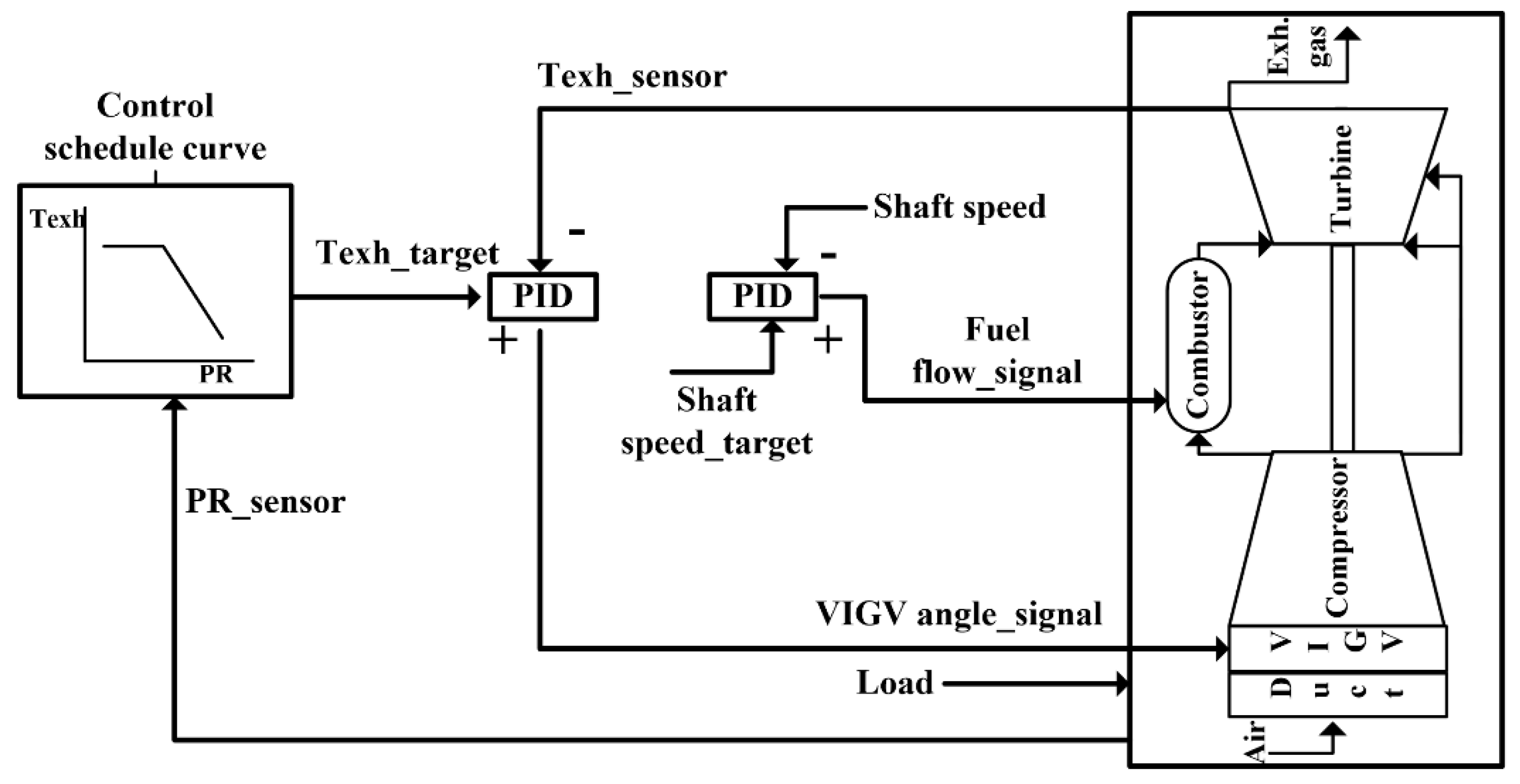
The conventional gas turbine control logic is illustrated in Figure 6. The control parameters are the turbine outlet temperature and rotational speed. The manipulated parameters to control the two control parameters to the target values are the VIGV angle and fuel flow rate. The target gas turbine is installed in a gas turbine/steam turbine combined cycle, and the TIT is maintained as high as possible to improve the cycle efficiency [49].
The airflow rate introduced to the compressor is adjusted using the VIGV to reduce the gas turbine power while maintaining a high TIT. However, it is difficult to adjust the VIGV with the TIT as a control parameter because the TIT is too high to measure in real gas turbines. As a result, the TIT is controlled indirectly by controlling it according to the exhaust gas control curve after measuring the exhaust gas temperature. The exhaust gas control curve is made by pre-scheduling the relationship of the exhaust gas temperature with the inlet temperature and pressure ratio, as shown in Figure 7. The rotational speed of gas turbines for power generation is controlled to a constant speed by adjusting the fuel flow rate to keep the electrical frequency.
The control process of the gas turbine using this control logic is as follows. The rotational speed of the shaft changes due to the imbalance between the generator load and gas turbine’s power. Accordingly, the fuel flow rate is adjusted through the controller to recover the rotational speed to the target value. Simultaneously, the target TET value is determined from the exhaust gas control curve using the gas turbine pressure, and the VIGV angle is adjusted to make the gas turbine TET meet the target value through the controller.
The new manipulated parameter (X) value in the next time step is calculated using the error of the control parameter (Y).
The proportional gain (KP), integral gain (KI), and derivative gain (KD) were optimized through trial and error to minimize the fluctuation of control variables.
3.2. Advanced Control Logic Using Black Box Models
3.2.1. Overview
Figure 8 shows the new control model. Two black box models were employed in the gas turbine control. The first black box model (black box model 1) is used in determining the target TET value for the gas turbine control, and the second black box model (black box model 2) is used in the ANN model predictive control (AMPC) to replace the PID control to transmit VIGV angle and fuel flow rate signals to the gas turbine.
3.2.2. Building Black Box Models Based on ANN
The ANN Toolbox [50] provided by MATLAB was used to develop the black box models of the gas turbine. In this study, a feed-forward neural network consisting of one hidden layer and one output layer was employed, which was verified to have high accuracy after being applied to a black box model for gas turbines in a previous study [51]. The Levenberg–Marquardt optimization algorithm, which is known to be the fastest training algorithm for a feed-forward neural network, was used in the black box model training.
Since the performance of a black box model is determined by the size of the hidden layer, multiple black box models were built while changing the size of the hidden layer. Then, the hidden layer size with the best performance was determined. The black box model performance was evaluated by comparing the mean squared errors (MSEs). The definition of the MSE is provided in Equation (17).
In this equation, n refers to the number of datasets used in training, y refers to the predicted value by the black box model, and z refers to the value of datasets used for validation and test.
The database used in the black box model training was built using the virtual gas turbine explained in Section 2.1, which simulates a real gas turbine. Datasets consisting of the input and output values in Table 2 were employed to train black box model 1, which was used to correct the target TET. To select an appropriate number of datasets, ambient temperature, compressor inlet pressure and load of the gas turbine were divided into 10, 10, and 100 sections, respectively. So, the total number of datasets for training black box model 1 was 104. To train black box model 2, which is used in the AMPC, datasets consisting of the input and output values in Table 3 were employed. Each of the five input parameters (i.e., ambient temperature, ambient pressure, fuel flow rate, relative VIGV angle, and rotational speed) was divided into 10 sections. So, the total number of datasets for training black box model 2 was 105.
We selected 10% of the entire datasets for training and used them for validation as well. Then, we created extra 10% datasets and used them for testing, which means that they were not used in the training. The size of hidden layer affects the performance of the black box model and is determined by the number of hidden neurons. In order to determine the optimal size of hidden layer, the number of hidden neurons was varied from 2 to 40. Figure 9 shows the results of the parametric study. Actually, there is no absolute rule of thumb for selecting the number of hidden neurons. In our case, the principle to select the appropriate number of hidden neurons was to make the MSE fall below 10−4, which seemed to be sufficiently low. As a result, the selected numbers of hidden neurons in black box models 1 and 2 were 6 and 30, respectively. The schematic diagrams of the final structures of the two black box models are illustrated in Figure 10.
3.2.3. Black Box Model for Correcting Control Target Value (Black Box Model 1)
As explained in Section 3.1, in the schedule-based control, the target TET value at every given load is determined by the control curve, which was prepared to relate the TET with the pressure ratio in advance. This control method has no problems when the gas turbine is in clean conditions without degradation. However, it would cause under- or over-firing of the engine if the pressure losses at the gas turbine inlet and outlet increase or if compressor fouling occurs. Such a problem will be demonstrated in Section 4.1. In brief, the variations in the actual operating conditions of the gas turbine, such as changes due to degradation, cannot be accommodated in the conventional control because the target TET is determined only by the pressure ratio signal and thus is invariable regardless of the changes in the operating conditions. As a result, it is nearly impossible to operate the gas turbine at an optimal condition in terms of performance.
In contrast, the black box model was used for correcting the control target value in the advanced control proposed in this study. In this control, the target TET was corrected to an optimal value in response to the change in the actual operating condition. The optimal target TET value was derived through a parametric simulation using the virtual gas turbine. As shown in Figure 8, black box model 1 derives the corrected target TET value once the input conditions are given. The purpose of the target TET correction is to maximize the gas turbine efficiency in varying operating conditions. As a result, the gas turbine can be controlled flexibly and optimally by considering the change in its operating condition.
3.2.4. Black Box Model for AMPC (Black Box Model 2)
In the conventional PID controls which are most widely used at present, instantly large overshoots and undershoots of the TIT and TET and large changes in rotational speed are unavoidable when the load fluctuates rapidly. This is because a PID control starts working only after an error between the target and measured values of the control parameter occurs.
In contrast, the second black box model in the Figure 8 was used for the AMPC to modulate the manipulated variables. Model predictive control generally has the advantage of increasing the response speed of the control through predictive control. However, it takes a long time to derive the manipulated variables because it uses a non-linear physical model [52]. In contrast, AMPC with a black box model can calculate at a faster rate [53].
In this study, to verify the usability of AMPC in gas turbines, a database was built, the black box model was trained according to a real operating environment, and the results of simulations were compared with actual operating data. The control sequence of the AMPC is as follows. The fuel flow rate and VIGV angle are controlled to satisfy the required load, target TET, and target shaft speed using black box model 2, and the objective function (Obj) value is derived as presented in Equation (18) by calculating 10 upcoming time steps.
In the equation, l refers to the number of predicting time steps and was set to 10. Q refers to the weighting factor of the rotational speed () and TET value, which are control parameters, and G refers to the weighting factor of the fuel flow rate and VIGV angle (), which are manipulated parameters. The , and values required proper tuning, and they were, respectively, found to be 7, 5, 1, and 1 through trial and error to minimize the fluctuation of variables and reduce the calculation load. The fuel flow rate and VIGV angle values of the next time step were determined to produce the minimum objective function value using an optimizer, and the values were sent to the gas turbine as control signals. Since MATLAB was used in the gas turbine modeling in this study, the Simplex optimization code [54] provided by MATLAB was used for the minimization of the objective function. As a result, the fluctuation of TET, TIT, and rotational speed was minimized when a rapid load change occurred.
4. Results and Discussion
4.1. Effect of Correcting Control Target Value Using a Black Box Model on Partial Load Performance
As mentioned in Section 3.2.3, conventional control logic (i.e., schedule-based control) has no problems when controlling the engine in clean conditions. However, when the performance is degraded, under- or over-firing occurs. To demonstrate this problem and present a solution, partial load operation was simulated while assuming an increase in the pressure loss at the compressor inlet, which is one of the typical problems that occur in gas turbines.
Figure 11 shows the partial load performance of the gas turbine in degraded conditions, where the inlet pressure loss was increased by 3%. The results are compared with those in clean conditions. With the degradation, the TIT is reduced slightly. The reduction is about 9 °C (0.7%) at the full load condition, where the VIGV of the compressor is fully opened. The compressor pressure ratio is maintained almost constant but the gas turbine power is reduced due to the decrease in the TIT. The changes in the operating conditions of the gas turbine can be explained with the aid of the temperature-entropy diagram illustrated in Figure 12, which compares the two full load operating points at clean and degraded conditions (A and B in Figure 11). The gas turbine cycle sequence is 1 → 2 → 3 → 4 in the clean condition. However, the cycle sequence changed to 1′ → 2′ → 3′ → 4 when the compressor inlet pressure loss occurs. Therefore, the operating pressure and temperature also change.
The pressure ratio of the gas turbine is determined by matching the compressor and turbine. The flow functions of the compressor and turbine are nearly constant according to the performance maps (see Figure 3 and Figure 4). Thus, the following equations are effective between the clean and degraded conditions.
If the compressor inlet pressure is reduced from to due to the inlet pressure loss, the inlet air flow rate decreases by the same rate ( → ). Accordingly, the inlet mass flow rate of the turbine also decreases by the same rate ( → ). Therefore, the turbine inlet mass flow rate decreases by about 3%. Even though the turbine inlet temperature ( → ) decreases, the reduction rate is very small (0.7%). So, the reduction in the inlet pressure of the turbine ( → ) is dominated by the reduction in inlet mass flow rate. Thus, the reduction rate of the turbine inlet pressure is nearly 3% as well. As a result, the compressor discharge pressure also decreases by the same rate ( → ). The net result is an almost constant compressor pressure ratio, even with the compressor inlet pressure loss:
Then, the TET is also maintained constant because the TET is a function of the compressor pressure ratio according to the control logic. Given a fixed turbine exit pressure (), the reduced turbine inlet pressure leads to a decrease in the turbine expansion ratio (). The net result in the turbine operation is that the TET remains the same but the expansion ratio decreases. Consequently, under-firing (reduction in TIT) takes place as illustrated in Figure 12: the reduction in TIT is exaggerated for illustration purpose. The combination of the reduced turbine explanation ratio and reduced TIT causes the turbine power to decrease. Of course, the efficiency also decreases. The impact of the under-firing on the partial load efficiency of the gas turbine is demonstrated in Figure 13. The decrease in TIT causes an efficiency reduction by 0.5%p (1.5%) on average.
To avoid the occurrence of under-firing, we corrected the TET target value using black box model 1. To compare the gas turbine control performance with that using the schedule-based control, a daily operation cycle of the gas turbine was set up. Figure 14 shows an example of the real hourly mean temperature distribution and electrical power demand curve in South Korea to set up the daily operation cycle. The simulation results of the one-day running gas turbine performance according to the demand curve of Figure 14 are displayed in Figure 15 and Figure 16. Because the gas turbine was set to operate while following the electrical power demand curve, Figure 15 verifies that both control logics simulated the gas turbine power very accurately. The power curves of both control methods (the upper curves in Figure 15) are almost the same as the power demand curve of Figure 14.
On the other hand, the operating temperatures are quite different between the two control methods. As shown in Figure 16, both the TET and TIT were maintained higher overall when applying the advanced control logic than when applying the conventional control logic. When the compressor loss increased by 3%p, the TIT was lower than the allowable limit in the conventional control logic. However, the TET is determined by the pressure ratio in the conventional control logic as mentioned above. As a result, although the compressor loss increased, the gas turbine was controlled following the scheduled TET. So, TIT was reduced by up to 20 °C from the allowable limit.
On the other hand, the advanced control logic could derive the most efficient corrected control target value of TET by considering the gas turbine conditions (components loss, components performance, and air conditions) and allowable ranges of the TET and TIT using the black box model. As a result, when applying the advanced control logic, the TIT and TET were higher, and the fluctuation of TIT was reduced. It can be found from Figure 16 that the TIT was kept at the allowable limit from 6 to 23 h because the target TET was determined to maintain a high TIT to maximize the gas turbine efficiency. From 0 to 5 h, the TIT was lower than the allowable limit because the TET reached the allowable value.
When applying the advanced control logic, as verified in Figure 15 (lower curves), the efficiency of the gas turbine was also higher by 0.12%p (0.35%) because the gas turbine efficiency increased due to the increase in the TIT. Furthermore, the increase in the TET would surely be positive in terms of the power output of a steam turbine driven by the gas turbine exhaust flow, leading to much better partial load efficiency of the combined cycle power plant.
4.2. Effect of Adopting AMPC on the Gas Turbine’s Response to Increased Ramp Rate
In addition to applying the black box model using an ANN to correct the control target values, we also used the black box model for AMPC by replacing the PID control. To compare the performance between the PID control and the AMPC, the dynamic behavior of the gas turbine upon a rapid increase in the load (power demand) was simulated using both controls. By referring to the literature [55], the load increase rate per unit time (ramp rate) was set to 30 MW/min. The time interval of dynamic behavior analysis was set to 0.1 s.
The changes in gas turbine power and rotational speed in Figure 17 verified that when applying AMPC, both the undershoot and overshoot were reduced, making the actual power follow the load better than with PID control. Comparing the results at 80 s when the variation in the load ends, it can be found that the gas turbine power did not overshoot when the AMPC was used. In contrast, when the PID was used, the gas turbine power increased by 1.8 MW (1.2%) showing a sensible overshoot before it converged to a steady state value.
The rotational speed changed due to the unbalance of the power and load of the gas turbine. With the PID control, the rotational speed reduced because the load is larger than the power at the specific moment when the load began to increase. Then, it began to increase when the load variation ended, converging to the target rotational speed. The maximum deviation of the rotational speed was 0.22%.
With the AMPC, however, the rotational speed increased earlier than when the load began to increase because the gas turbine power increased in advance owing to the predictive control. Then, it began to decrease when the load variation ended, converging to the target rotational speed. The maximum deviation of the rotational speed was 0.061%, which was only one-fourth of that of the PID control.
Figure 18 verifies that when using the PID control, the TIT and TET are higher than in the AMPC by up to 1.4% and 1.9%, respectively. The reason for this was that the rotational speed was reduced due to the unbalance of the gas turbine power and load. Thus, the fuel flow rate was increased to recover the reduced rotational speed back to the target value. Accordingly, the TIT and TET momentarily increased sharply at the moment when the load began to increase showing an overshoot and then converged to a steady state value.
In contrast, with the AMPC, the TIT and TET converged to a steady state value smoothly. This means that there is practically no overshoot. It is clearly shown in Figure 19 that the changes in both the VIGV angle and fuel flow rate, which are manipulated variables, begin earlier with the AMPC than the PID control. This is due to the inherent advantage of the AMPC. The AMPC predicts the 10 upcoming time steps in advance, whereas The PID control is initiated only after a difference between the measured (actual) and target values occurs. With the AMPC, once the difference between measured and target values is predicted, it minimizes the deviation of the rotation speed, TET, and TIT.
To demonstrate the advantage of the AMPC in a harsher control environment, a case where the where the ramp rate was doubled (i.e., 60 MW/min) was simulated, and the results are illustrated in Figure 20, Figure 21 and Figure 22. When using the PID control, the overshoot of the gas turbine power also increased significantly: it increased by 3 MW (2%) from 150 MW before it converged to a steady state value. The maximum deviation of the rotational speed increased to 0.41%. The maximum variations of the TIT and TET also increased to 3% and 4%, respectively. When using the AMPC, the maximum deviation of the rotational speed increased only to 0.13%, which was much smaller than that when using the PID control, and the maximum deviations of the TET and TIT were also much smaller in comparison to the case with the PID control.
As a result, when the ramp rate was doubled (60 MW/min), the maximum deviation of the operation variables such as the rotational speed, TIT, and TET was almost doubled when using the PID control. In contrast, when using the AMPC, both the TIT and TET were controlled smoothly almost without overshoots. No sensible difference was observed in comparison to the lower ramp rate case. The maximum deviation of the rotational speed was almost doubled but is still much smaller than that of the PID control. This result verified that the ramp rate can be increased while significantly reducing the fluctuation of main parameters by using the advanced control logic compared to that using the conventional control logic.
5. Conclusions
This study proposed advanced control logic with two ANN-based black box models to overcome the drawbacks of the conventional schedule-based control. The main results and conclusions are summarized as follows:
When applying the conventional control method, under-firing occurs, resulting in a reduction in efficiency of the gas turbine if problems arise, such as increases in the inlet and outlet pressure losses. In contrast, the advanced control is performed by correcting the target value (TET) in the gas turbine using a black box model based on an ANN. Operations can be achieved while maintaining the TIT and TET of the gas turbine at the optimal values within the allowable range. Moreover, higher TET, TIT, and efficiency can be achieved compared to those achieved by applying the schedule-based control. Furthermore, the increase in TET of the gas turbine may lead to an increase in the efficiency of larger systems when applied to a combined cycle and combined heat and power systems.
When applying the advanced control logic using the AMPC, the maximum deviation of the rotational speed was reduced by 1/4 compared to the conventional control using the PID because the AMPC can achieve optimal control by predicting the result in advance. The results of the AMPC also verified that the maximum fluctuations of the TIT and TET were also significantly reduced. Moreover, even when the ramp rate was doubled, all deviations of the rotational speed, TET, and TIT were smaller than those of PID control.
The significance of the new control is high in various aspects. Firstly, the overall fuel economy in gas turbine operation would increase because of the improved partial load efficiency enabled by the optimized control. Secondly, the reduction in the deviation of the rotational speed is beneficial in increasing the quality of the generated electricity from the gas turbine by reducing the frequency fluctuation. Thirdly, the reduction in the maximum fluctuations of the TIT and TET extend the life of high-temperature parts. These advantages would be more eminent as the operating environment of the gas turbines becomes harsher as the penetration of variable renewable energy increases.
This study has focused on performance optimization. However, consideration of the impact of gas turbine operation on the emission such as NOx and CO would be important as well because the environmental regulation in the power generation industry is becoming increasingly strict day by day. Therefore, a study on the influence of the advanced control logic on the gas turbine emissions needs to be performed as subsequent research.
Author Contributions
Conceptualization, S.W.M. and T.S.K., methodology, S.W.M. and T.S.K., Software, S.W.M., validation, S.W.M., formal analysis, S.W.M., investigation, S.W.M., resources, T.S.K., data curation, S.W.M., writing—original draft, S.W.M. and T.S.K., writing—review and editing, S.W.M. and T.S.K., supervision, T.S.K., project administration, T.S.K., funding acquisition, T.S.K. All authors have read and agreed to the published version of the manuscript.
Funding
This work was supported by the Korea Institute of Energy Technology Evaluation and Planning (KETEP) and the Ministry of Trade, Industry and Energy (MOTIE) of the Republic of Korea (No.20193310100050).
Conflicts of Interest
The authors declare no conflict of interest.
Nomenclature
| a | Constant of chemical species |
| b | Constant of chemical species |
| C | Rotor coolant charging factor |
| cp | Specific heat at constant pressure (kJ/kg·K) |
| e | error |
| G | Manipulated variables weighting factor |
| h | Specific enthalpy (kJ/kg) |
| I | Inertia (kg·m2) |
| K | Gain value |
| L | Load (MW) |
| M | Flow function (kg·K0.5/kN·s) |
| Mass flow rate (kg/s) | |
| n | Number of data |
| p | Pressure (kPa) |
| PR | Pressure ratio |
| Obj | Object function |
| Q | Control variables weighting factor |
| R | Gas constant (kJ/kg·K) |
| s | Specific entropy (kJ/kg) |
| t | Time (sec) |
| T | Temperature (K) |
| Power (MW) | |
| X | Manipulated variables |
| x | Value of data |
| Y | Control variables |
| y | Value of predicting data |
| z | Value of training and testing data |
| Relative inlet guide vane angle | |
| Efficiency | |
| Rotation speed (RPM) | |
| Semi-non-dimensional rotation speed (K0.5/RPM) | |
| Subscripts | |
| 1,2,3,4 | Locations in the gas turbine |
| AUX loss | Auxiliary loss |
| comb | Combustor |
| comp | Compressor |
| coolant | Coolant flow |
| corrected | Corrected value |
| d | Design state |
| D | Derivative |
| exh. | Turbine exhaust |
| f | Fuel |
| field | Field data |
| GT | Gas turbine |
| I | Integral |
| i | index |
| in | Inlet |
| initial | Initial value |
| l | Number of predicting time steps |
| n | Number of data |
| out | Outlet |
| P | Proportional |
| s | Isentropic |
| simulation | Simulation data |
| t | Time step |
| target | Control target value |
| turb | Turbine |
| Abbreviations | |
| ANN | Artificial neural network |
| AMPC | ANN model predictive control |
| MSE | Mean squared error |
| MPC | Model predictive control |
| P2G | Power to gas |
| TIT | Turbine inlet temperature |
| TET | Turbine exhaust temperature |
| VIGV | Variable inlet guide vane |
References
- Shahbaz, M.; Raghutla, C.; Chittedi, K.R.; Jiao, Z.; Vo, X.V. The Effect of Renewable Energy Consumption on Economic Growth: Evidence from the Renewable Energy Country Attractive Index. Energy 2020, 207, 118162. [Google Scholar] [CrossRef]
- Wang, Q.; Wang, L. Renewable energy consumption and economic growth in OECD countries: A nonlinear panel data analysis. Energy 2020, 207, 118200. [Google Scholar] [CrossRef]
- Sarker, E.; Seyedmahmoudian, M.; Jamei, E.; Horan, B.; Stojcevski, A. Optimal Management of Home Loads with Renewable Energy Integration and Demand Response Strategy. Energy 2020, 210, 118602. [Google Scholar] [CrossRef]
- Chettibi, N.; Mellit, A. Intelligent Control Strategy for a Grid Connected PV/SOFC/BESS Energy Generation System. Energy 2018, 147, 239–262. [Google Scholar] [CrossRef]
- Pena-Bello, A.; Barbour, E.; Gonzalez, M.C.; Yilmaz, S.; Patel, M.K.; Parra, D. How Does the Electricity Demand Profile Impact the Attractiveness of PV-Coupled Battery Systems Combining Applications? Energies 2020, 13, 4038. [Google Scholar] [CrossRef]
- Raugei, M.; Peluso, A.; Leccisi, E.; Fthenakis, V. Life-Cycle Carbon Emissions and Energy Return on Investment for 80% Domestic Renewable Electricity with Battery Storage in California (U.S.A.). Energies 2020, 13, 3934. [Google Scholar] [CrossRef]
- Aktaş, A.; Kırçiçek, Y.A. Novel Optimal Energy Management Strategy for Offshore Wind/Marine Current/Battery/Ultracapacitor Hybrid Renewable Energy System. Energy 2020, 199, 117425. [Google Scholar] [CrossRef]
- Sikorski, T.; Jasiński, M.; Ropuszyńska-Surma, E.; Węglarz, M.; Kaczorowska, D.; Kostyla, P.; Leonowicz, Z.; Lis, R.; Rezmer, J.; Rojewski, W.; et al. A Case Study on Distributed Energy Resources and Energy-Storage Systems in a Virtual Power Plant Concept: Technical Aspects. Energies 2020, 13, 3086. [Google Scholar] [CrossRef]
- Zhao, H.; Wu, Q.; Hu, S.; Xu, H.; Rasmussen, C.N. Review of Energy Storage System for Wind Power Integration Support. Appl. Energy 2015, 137, 545–553. [Google Scholar] [CrossRef]
- Kim, E.H.; Park, Y.G.; Roh, J.H. Competitiveness of Open-Cycle Gas Turbine and Its Potential in the Future Korean Electricity Market with High Renewable Energy Mix. Energy Policy 2019, 129, 1056–1069. [Google Scholar] [CrossRef]
- Isaiah, T.G.; Dabbashi, S.; Bosak, D.; Sampath, S.; Di Lorenzo, G.; Pilidis, P. Life Analysis of Industrial Gas Turbines Used as a Back-Up to Renewable Energy Sources. Procedia CIRP 2015, 38, 239–244. [Google Scholar] [CrossRef] [Green Version]
- Zhou, S.; Sun, K.; Wu, Z.; Gu, W.; Wu, G.; Li, Z.; Li, J. Optimized Operation Method of Small and Medium-Sized Integrated Energy System for P2G Equipment under Strong Uncertainty. Energy 2020, 199, 117269. [Google Scholar] [CrossRef]
- Belderbos, A.; Valkaert, T.; Bruninx, K.; Delarue, E.; D’haeseleer, W. Facilitating Renewables and Power-to-Gas via Integrated Electrical Power-Gas System Scheduling. Appl. Energy 2020, 275, 115082. [Google Scholar] [CrossRef]
- Jeong, J.H.; Yi, J.H.; Kim, T.S. Analysis of Options in Combining Compressed Air Energy Storage with a Natural Gas Combined Cycle. J. Mech. Sci. Technol. 2018, 32, 3453–3464. [Google Scholar] [CrossRef]
- Kim, M.J.; Kim, T.S. Feasibility Study on the Influence of Steam Injection in the Compressed Air Energy Storage System. Energy 2017, 141, 239–249. [Google Scholar] [CrossRef]
- Tsoutsanis, E.; Meskin, N.; Benammar, M.; Khorasani, K. A Dynamic Prognosis Scheme for Flexible Operation of Gas Turbines. Appl. Energy 2016, 164, 686–701. [Google Scholar] [CrossRef] [Green Version]
- Huang, Z.; Yang, C.; Yang, H.; Ma, X. Off-Design Heating/Power Flexibility for Steam Injected Gas Turbine Based CCHP Considering Variable Geometry Operation. Energy 2018, 165, 1048–1060. [Google Scholar] [CrossRef]
- Barelli, L.; Ottaviano, A. Supercharged Gas Turbine Combined Cycle: An Improvement in Plant Flexibility and Efficiency. Energy 2015, 81, 615–626. [Google Scholar] [CrossRef]
- Buschmeier, M.; Kleinwächter, T.; Feldmüller, A.; Köhne, P.; Energy, S. Improving Flexibility of the Combined Cycle Power Plant Hamm Uentrop to Cover the Operational Profiles of the Future. In Proceedings of the POWER-GEN Europe, Cologne, Germany, 3–5 June 2014. [Google Scholar]
- Kim, T.S. Comparative Analysis on the Part Load Performance of Combined Cycle Plants Considering Design Performance and Power Control Strategy. Energy 2004, 29, 71–85. [Google Scholar] [CrossRef]
- Rowen, W.I. Operating Characteristics of Heavy-Duty Gas Turbines in Utility Service. In Proceedings of the ASME 1988 International Gas Turbine and Aeroengine Congress and Exposition, Amsterdam, The Netherlands, 6–9 June 1988. ASME paper 88-GT-150. [Google Scholar]
- Rowen, W.I. Simplified Mathematical Representations of Single Shaft Gas Turbines in Mechanical Drive Service. In Proceedings of the ASME 1992 International Gas Turbine and Aeroengine Congress and Exposition, Cologne, Germany, 1–4 June 1992. ASME paper 92-GT-022. [Google Scholar]
- Tavakoli, M.R.B.; Vahidi, B.; Gawlik, W. An Educational Guide to Extract the Parameters of Heavy Duty Gas Turbines Model in Dynamic Studies Based on Operational Data. IEEE Trans. Power Syst. 2009, 24, 1366–1374. [Google Scholar] [CrossRef]
- Lee, J.H.; Kim, T.S. Novel Performance Diagnostic Logic for Industrial Gas Turbines in Consideration of Over-Firing. J. Mech. Sci. Technol. 2018, 32, 5947–5959. [Google Scholar] [CrossRef]
- Kim, M.J.; Kim, T.S. Integration of Compressed Air Energy Storage and Gas Turbine to Improve the Ramp Rate. Appl. Energy 2019, 247, 363–373. [Google Scholar] [CrossRef]
- Lin, H.; Leon, J.I.; Luo, W.; Marquez, A.; Liu, J.; Vazquez, S.; Franquelo, L.G. Integral Sliding-Mode Control-Based Direct Power Control for Three-Level NPC Converters. Energies 2020, 13, 227. [Google Scholar] [CrossRef] [Green Version]
- Krzywanski, J.A. General Approach in Optimization of Heat Exchangers by Bio-Inspired Artificial Intelligence Methods. Energies 2019, 12, 4441. [Google Scholar] [CrossRef] [Green Version]
- Krzywanski, J.; Fan, H.; Feng, Y.; Shaikh, A.R.; Fang, M.; Wang, Q. Genetic algorithms and neural networks in optimization of sorbent enhanced H2 production in FB and CFB gasifiers. Energy Convers. Manag. 2018, 171, 1651–1661. [Google Scholar] [CrossRef]
- Lin, H.; Sun, Q. Crude Oil Prices Forecasting: An Approach of Using CEEMDAN-Based Multi-Layer Gated Recurrent Unit Networks. Energies 2020, 13, 1543. [Google Scholar] [CrossRef] [Green Version]
- Stojčić, M.; Stjepanović, A.; Stjepanović, Đ. ANFIS model for the prediction of generated electricity of photovoltaic modules. Decis. Mak. Appl. Manag. Eng. 2019, 2, 35–48. [Google Scholar] [CrossRef]
- MathWorks, 2019, MATLAB R2019b. Available online: https://mathworks.com/products/matlab.html (accessed on 31 October 2020).
- Kim, M.J.; Kim, J.H.; Kim, T.S. Program Development and Simulation of Dynamic Operation of Micro Gas Turbines. Appl. Therm. Eng. 2016, 108, 122–130. [Google Scholar] [CrossRef]
- Kim, J.H.; Kim, T.S.; Moon, S.J. Development of a Program for Transient Behavior Simulation of Heavy-Duty Gas Turbines. J. Mech. Sci. Technol. 2016, 30, 5817–5828. [Google Scholar] [CrossRef]
- Kim, M.J.; Kim, J.H.; Kim, T.S. The effects of internal leakage on the performance of a micro gas turbine. Appl. Energy 2018, 212, 175–184. [Google Scholar] [CrossRef]
- Kang, D.W.; Kim, T.S. Model-Based Performance Diagnostics of Heavy-Duty Gas Turbines Using Compressor Map Adaptation. Appl. Energy 2018, 212, 1345–1359. [Google Scholar] [CrossRef]
- Gay, R.R.; Palmer, C.A.; Erbes, M.R. Power Plant Performance Monitoring; Techniz Books International: New Delhi, India, 2006; pp. 110–116. ISBN 0-9755876-0-9. [Google Scholar]
- Moon, S.W.; Kwon, H.M.; Kim, T.S.; Kang, D.W.; Sohn, J.L. A Novel Coolant Cooling Method for Enhancing the Performance of the Gas Turbine Combined Cycle. Energy 2018, 160, 625–634. [Google Scholar] [CrossRef]
- Lee, J.H.; Kim, T.S.; Kim, E. Prediction of Power Generation Capacity of a Gas Turbine Combined Cycle Cogeneration Plant. Energy 2017, 124, 187–197. [Google Scholar] [CrossRef]
- McBride, B.J. NASA Glenn Coefficients for Calculating Thermodynamic Properties of Individual Species; National Aeronautics and Space Administration, John H. Glenn Research Center at Lewis Field: Cleveland, OH, USA, 2002.
- Moran, M.J.; Shapiro, H.N.; Boettner, D.D.; Bailey, M.B. Fundamentals of Engineering Thermodynamics; John Wiley & Sons: Hoboken, NJ, USA, 2010; ISBN 978-0470495902. [Google Scholar]
- Saravanamuttoo, H.I.; Rogers, G.F.C.; Cohen, H. Gas Turbine Theory; Pearson Education: London, UK, 2001; ISBN 978-1292093093. [Google Scholar]
- Song, T.W.; Kim, T.S.; Kim, J.H.; Ro, S.T. Performance Prediction of Axial Flow Compressors Using Stage Characteristics and Simultaneous Calculation of Interstage Parameters. Proc. Inst. Mech. Eng. Part A J. Power Energy 2001, 215, 89–98. [Google Scholar] [CrossRef]
- Lee, J.J.; Kang, D.W.; Kim, T.S. Development of a Gas Turbine Performance Analysis Program and Its Application. Energy 2011, 36, 5274–5285. [Google Scholar] [CrossRef]
- Kim, J.H.; Kim, T.S. Development of a Program to Simulate the Dynamic Behavior of Heavy-Duty Gas Turbines during the Entire Start-up Operation Including Very Early Part. J. Mech. Sci. Technol. 2019, 33, 4495–4510. [Google Scholar] [CrossRef]
- Choi, B.S.; Kim, M.J.; Ahn, J.H.; Kim, T.S. Influence of a Recuperator on the Performance of the Semi-Closed Oxy-Fuel Combustion Combined Cycle. Appl. Therm. Eng. 2017, 124, 1301–1311. [Google Scholar] [CrossRef]
- Kim, J.H.; Kim, T.S. A New Approach to Generate Turbine Map Data in the Sub-Idle Operation Regime of Gas Turbines. Energy 2019, 173, 772–784. [Google Scholar] [CrossRef]
- Palmer, C.A.; Erbes, M.R. Simulation Methods Used to Analyze the Performance of the GE PG6541B Gas Turbine Utilizing Low Heating Value Fuels. In Proceedings of the CONF-941024, New York, NY, USA, 25–27 October 1994. [Google Scholar]
- California Energy Commission. Redondo Beach Energy Project-Appendix 3A CAISO Interconnection Request and Payment; 2012; Report for certification, LA, CA. Available online: https://ww2.energy.ca.gov/sitingcases/redondo_beach/documents/applicant/AFC/Vol_2/ (accessed on 31 October 2020).
- Rowen, W.I.; Van Housen, R.L. Gas turbine airflow control for optimum heat recovery. J. Eng. Power 1983, 105, 72–79. [Google Scholar] [CrossRef]
- Beale, M.H.; Hagan, M.T.; Demuth, H.B. Neural network toolbox. User’s Guide. MathWorks 2010, 2, 77–81. [Google Scholar]
- Kim, M.J.; Kim, T.S.; Flores, R.J.; Brouwer, J. Neural-Network-Based Optimization for Economic Dispatch of Combined Heat and Power Systems. Appl. Energy 2020, 265, 114785. [Google Scholar] [CrossRef]
- Kim, J.S.; Powell, K.M.; Edgar, T.F. Nonlinear Model Predictive Control for a Heavy-Duty Gas Turbine Power Plant. In Proceedings of the 2013 American Control Conference, Washington, DC, USA, 17–19 June 2013; pp. 2952–2957. [Google Scholar]
- Asgari, H.; Chen, X. Gas Turbines Modeling, Simulation, and Control: Using Artificial Neural Networks; CRC Press: Boca Raton, FL, USA, 2015; pp. 133–135. [Google Scholar]
- Lagarias, J.C.; Reeds, J.A.; Wright, M.H.; Wright, P.E. Convergence properties of the Nelder–Mead simplex method in low dimensions. SIAM J. Optim. 1998, 9, 112–147. [Google Scholar] [CrossRef] [Green Version]
- General Electric Company GE 7FA Power Plant Fact Sheet 2020; GE32930A. Available online: http://www.ge.com/power/gas/gas-turbines/7f-05 (accessed on 30 October 2020).
Figure 1.
Structure of the virtual gas turbine.

Figure 2.
Configuration of the gas turbine for simulation.

Figure 3.
Compressor performance map.

Figure 4.
Compressor performance map.

Figure 5.
Variation in gas turbine parameters with load: comparison between simulation and field data.
Figure 5.
Variation in gas turbine parameters with load: comparison between simulation and field data.

Figure 6.
Conventional schedule-based control logic.

Figure 7.
The control curve for the conventional schedule-based control.

Figure 8.
Advanced control logic using artificial neural network (ANN) black box models.

Figure 9.
Variation in mean squared error with the number of hidden neurons.

Figure 10.
Configuration of black box models based on ANN.

Figure 11.
Partial load parameter variations in the schedule-based control: impact of the compressor inlet pressure loss.
Figure 11.
Partial load parameter variations in the schedule-based control: impact of the compressor inlet pressure loss.

Figure 12.
Changes in the cycle parameters on the temperature-entropy diagram due to the compressor inlet pressure loss.
Figure 12.
Changes in the cycle parameters on the temperature-entropy diagram due to the compressor inlet pressure loss.

Figure 13.
Variations in the partial load efficiency with the schedule-based control.

Figure 14.
Example of the variations in ambient temperature and electric power demand during a spring day in South Korea.
Figure 14.
Example of the variations in ambient temperature and electric power demand during a spring day in South Korea.

Figure 15.
Variations in power production and efficiency of the gas turbine during a day.

Figure 16.
Simulated variations in TET and TIT of the gas turbine during a day.

Figure 17.
Simulated variations in gas turbine power and rotational speed with increasing load (ramp rate: 30 MW/min).
Figure 17.
Simulated variations in gas turbine power and rotational speed with increasing load (ramp rate: 30 MW/min).

Figure 18.
Simulated variations in gas TIT and TET with increasing load (ramp rate: 30 MW/min).

Figure 19.
Simulated variations in fuel flow rate and VIGV angle with increasing load (ramp rate: 30 MW/min).
Figure 19.
Simulated variations in fuel flow rate and VIGV angle with increasing load (ramp rate: 30 MW/min).

Figure 20.
Simulated variations in gas turbine power and rotational speed with increasing load (ramp rate: 60 MW/min).
Figure 20.
Simulated variations in gas turbine power and rotational speed with increasing load (ramp rate: 60 MW/min).

Figure 21.
Simulated variations in gas TIT and TET with increasing load (ramp rate: 60 MW/min).

Figure 22.
Simulated variations in fuel flow rate and VIGV angle with increasing load (ramp rate: 60 MW/min).
Figure 22.
Simulated variations in fuel flow rate and VIGV angle with increasing load (ramp rate: 60 MW/min).


Table 1.
Specifications of the target gas turbine.
| Parameters | 7FA | Type of the Parameter in the Simulation | |
|---|---|---|---|
| Field Data | Modeling | ||
| Ambient temperature (°C) | 15 | 15 | Input |
| Ambient pressure (kPa) | 101.3 | 101.3 | Input |
| Fuel flow rate (kg/s) | 9.03 | 9.03 | Input |
| Pressure ratio | 15.0 | 15.0 | Input |
| Compressor polytropic efficiency (%) | 0.89 | 0.89 | input |
| Turbine inlet temperature (°C) | Unknown | 1420 | Assumed input |
| Turbine polytropic efficiency (%) | Unknown | 0.88 | Assumed input |
| Total coolant flow relative to inlet air (%) | Unknown | 20 | Calculated |
| Exhaust gas flow rate (kg/s) | 420 | 420 | Input |
| Exhaust gas temperature (°C) | 603 | 603 | Calculated |
| Net power (MW) | 160 | 160 | Calculated |
| Gas turbine LHV efficiency (%) | 36 | 36 | Calculated |
Table 2.
Variation ranges of parameters for making database for black box model 1.
| Input Data | Output Data | |
|---|---|---|
| Parameters | Range (Unit) | Parameters(unit) |
| Ambient temperature | −15~30 (°C) | Corrected target TET (°C) |
| Compressor inlet pressure | 95~105 (kPa) | |
| Load of gas turbine | 50~100 (%) | |
Table 3.
Variation ranges of parameters for making database for black box model 2.
| Input Data | Output Data | |
|---|---|---|
| Parameters | Range (unit) | Parameters (unit) |
| Ambient temperature | −15~30 (°C) | Inlet flow rate (kg/s) |
| Ambient Pressure | 95~105 (kPa) | Pressure ratio |
| Fuel flow rate | 7~9.5 (kg/s) | TET (°C) |
| Relative VIGV angle | 50~100 | TIT (°C) |
| Rotational speed | 3500~3700 (RPM) | Gas turbine power (kW) |
Publisher’s Note: MDPI stays neutral with regard to jurisdictional claims in published maps and institutional affiliations. |
© 2020 by the authors. Licensee MDPI, Basel, Switzerland. This article is an open access article distributed under the terms and conditions of the Creative Commons Attribution (CC BY) license (http://creativecommons.org/licenses/by/4.0/).
Share and Cite
MDPI and ACS Style
Moon, S.W.; Kim, T.S. Advanced Gas Turbine Control Logic Using Black Box Models for Enhancing Operational Flexibility and Stability. Energies 2020, 13, 5703. https://doi.org/10.3390/en13215703
AMA Style
Moon SW, Kim TS. Advanced Gas Turbine Control Logic Using Black Box Models for Enhancing Operational Flexibility and Stability. Energies. 2020; 13(21):5703. https://doi.org/10.3390/en13215703
Chicago/Turabian StyleMoon, Seong Won, and Tong Seop Kim. 2020. "Advanced Gas Turbine Control Logic Using Black Box Models for Enhancing Operational Flexibility and Stability" Energies 13, no. 21: 5703. https://doi.org/10.3390/en13215703
Note that from the first issue of 2016, this journal uses article numbers instead of page numbers. See further details here.