
Performance Enhancement of Proposed Namaacha Wind Farm by Minimising Losses Due to the Wake Effect: A Mozambican Case Study


1
Faculty of Engineering and the Built Environment, Department of Mechanical and Mechatronics Engineering, Tshwane University of Technology, Private Bag X680, Pretoria 0001, South Africa
2
Faculty of Engineering and the Built Environment, Department of Electrical Engineering, Tshwane University of Technology, Private Bag X680, Pretoria 0001, South Africa
*
Author to whom correspondence should be addressed.
Energies 2021, 14(14), 4291; https://doi.org/10.3390/en14144291
Submission received: 30 May 2021
/
Revised: 21 June 2021
/
Accepted: 30 June 2021
/
Published: 16 July 2021
(This article belongs to the Special Issue Advances in Wind Farm Layout Optimization)
Abstract
:District of Namaacha in Maputo Province of Mozambique presents a high wind potential, with an average wind speed of around 7.5 m/s and huge open fields that are favourable to the installation of wind farms. However, in order to make better use of the wind potential, it is necessary to evaluate the operating conditions of the turbines and guide the independent power producers (IPPs) on how to efficiently use wind power. The investigation of the wind farm operating conditions is justified by the fact that the implementation of wind power systems is quite expensive, and therefore, it is imperative to find alternatives to reduce power losses and improve energy production. Taking into account the power needs in Mozambique, this project applied hybrid optimisation of multiple energy resources (HOMER) to size the capacity of the wind farm and the number of turbines that guarantee an adequate supply of power. Moreover, considering the topographic conditions of the site and the operational parameters of the turbines, the system advisor model (SAM) was applied to evaluate the performance of the Vestas V82-1.65 horizontal axis turbines and the system’s power output as a result of the wake effect. For any wind farm, it is evident that wind turbines’ wake effects significantly reduce the performance of wind farms. The paper seeks to design and examine the proper layout for practical placements of wind generators. Firstly, a survey on the Namaacha’s electricity demand was carried out in order to obtain the district’s daily load profile required to size the wind farm’s capacity. Secondly, with the previous knowledge that the operation of wind farms is affected by wake losses, different wake effect models applied by SAM were examined and the Eddy–Viscosity model was selected to perform the analysis. Three distinct layouts result from SAM optimisation, and the best one is recommended for wind turbines installation for maximising wind to energy generation. Although it is understood that the wake effect occurs on any wind farm, it is observed that wake losses can be minimised through the proper design of the wind generators’ placement layout. Therefore, any wind farm project should, from its layout, examine the optimal wind farm arrangement, which will depend on the wind speed, wind direction, turbine hub height, and other topographical characteristics of the area. In that context, considering the topographic and climate features of Mozambique, the study brings novelty in the way wind farms should be placed in the district and wake losses minimised. The study is based on a real assumption that the project can be implemented in the district, and thus, considering the wind farm’s capacity, the district’s energy needs could be met. The optimal transversal and longitudinal distances between turbines recommended are 8Do and 10Do, respectively, arranged according to layout 1, with wake losses of about 1.7%, land utilisation of about 6.46 Km2, and power output estimated at 71.844 GWh per year.
1. Introduction
The growth in power consumption worldwide, combined with the issue of climate changes that concerns all the stakeholders across the globe, has driven renewable energies to play an important role in mitigating environmental impacts and providing universal power access to populations suffering from power poverty [1,2,3,4,5,6]. Although many countries have a sturdy interest in renewable power technologies, there are still major challenges in the implementation of these alternative energy generations [7,8]. Wind power is a prominent source and has aroused massive attention in the last past decade, but its low capacity factor associated with its high cost of the initial investment, in addition to its maintenance [9,10], has necessitated research to continue with improvement of its performance. Moreover, the unpredictable dynamic behaviour of a wind turbine has not yet been possible to predict properly, considering uncertainties of various operating parameters [1,11,12]. The overall efficiency of a wind system depends on several factors, such as aerodynamic and mechanical characteristics of the wind turbine and operating parameters of the electric generator and other auxiliary electric components [13,14]. A selected wind site requires a proper layout for the installation and commissioning of wind generators. There is a research gap in the published literature concerning the layout optimisation for minimising losses due to wake effects to maximise energy output. The following key factors affect the performance of wind for energy generation systems:
- ▪
- ▪
- The wind turbine’s design such as rotor´s diameter, blade geometry, and wind tower´s height—the fundamentals of aerodynamics have been decisive for the advance of wind turbines [18]. A number of numerical modelling challenges are present in the design of wind turbines, with respect to the aerodynamics of the rotor and blades and stability of the tower under wind gusts and oscillations [17,19]. Depending on the type of turbine, its performance is influenced by other design parameters such as the number of blades and rotor orientation [14,20,21,22].
- ▪
- The wind farm layout such as the site´s topographic conditions, the distance between two consecutive turbines, and the erection layout (linear or scattered)—depending on the local wind conditions of the wind site, the design can lead to power loss due to wake effect on the wind farm. Wind turbines’ wake effects significantly reduce the performance of downstream wind turbines [7,23,24,25,26]. With the increase in the number of turbines downstream, the influence of the wake effect and load of airflow generated tends to be more significant [7,27].
With regard to the subject of wake effect minimisation, Sun et al. [7] summarised the results of wake losses measurement experiments in distinct wind farms. In general, the experimental measurement results proved that for high wind speeds, the deficits in the wind speed reached approximately 45%, 35%, and 5% at distances of 3Do, 3.5Do, and 5Do, respectively.
In addition to the influence of wind speed and distance between turbines, the tests also demonstrated that the wake losses are influenced by the number of turbines in the wind farm as well as the turbine’s rotor diameter Do and hub height. For 20 turbines with a rotor diameter of 76 m, a hub height of 64 m, and turbines spacing of 2.4 Do, results showed that for the wind speed of 11 m/s, the turbulence intensity is about 6.5%. Fei et al. [23] investigated the influence of the rotor diameter on wake width and depth. Results proved that with the increase of downwind distance, the wake width and depth increase regardless of the rotor diameter. However, the growth magnitude is diverse, and thus, the greater the diameter is, the lower the growth magnitude becomes.
Dhiman et al. [25] applied a bilateral wake model derived from two benchmark models, namely, Jensen’s and Frandsen’s variation models, to evaluate the wind speed prediction in the presence of wakes for two distinct wind farms composed of 5 turbines (layout A) and 15 turbines (layout B). Results revealed that for layout A, the prediction accuracy improved by 10.56%, 10.05%, and 10.48% when the inputs to the forecasting model are from Jensen’s, Frandsen’s, and bilateral wake models, respectively. Similarly, for layout B, an improvement in prediction accuracy by 20.47%, 8.37%, and 46.88% was when the inputs to the forecasting model are from Jensen’s, Frandsen’s, and bilateral wake model, respectively.
Ge et al. [26] investigated the interaction between the wind turbine wake and a building array applying large eddy simulation. Results showed that the urban district can considerably influence the development of the turbine wake, and thus, this proves the influence of the surrounding environment and landscape on the wind farm performance. Tao et al. [27] examined the performance of three wind farms composed of different numbers of turbines (layout C = 25 turbines, layout D = 45, and layout E = 60). Results demonstrated that with the increase of turbines in the farm, wake losses increase. Note that the results of the studies display diverse trends and emphasise the novelty existing in each wind farm performance assessment as a particular case.
2. Performance Analysis of Wind Technology Aerodynamics
Thus far, in the field of power generation, different models of wind turbines have been developed. In general, according to the rotation direction, wind turbines can be classified into two major types: horizontal axis wind turbine (HAWT) and vertical axis wind turbine (VAWT) [11,12,28,29]. The aerodynamic performance of the wind turbine depends greatly on the power extracted from the wind mass and the shape of the blade’s cross section and thus is linked to the power coefficient Cp, which expresses the amount of power extracted from the wind [30]. Wind power turbines are placed in wide, extended, fluxes of air movement. The air that passes through the wind turbine cannot, therefore, be deflected into regions where there is no air already and so there are individual limits to wind turbine efficiency.
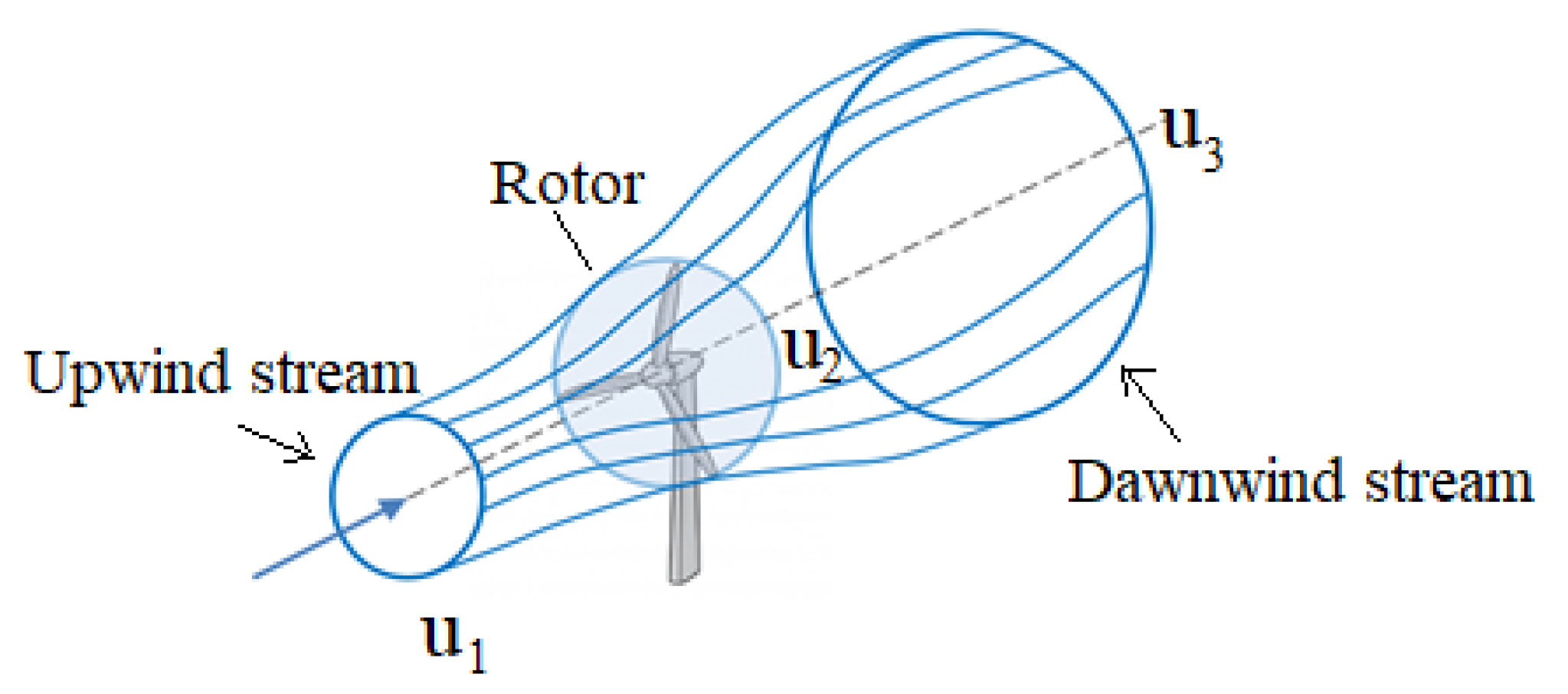
According to Steiger [31], in Figure 1, the upwind stream approaching the turbine flows undisturbed with velocity , and the downwind stream transited through the turbine and flowing with velocity is substantially slowed. Considering that at the disk, the flow velocity is the average of the upstream and downstream velocities and , it can be expressed as follows:
Due to the reduction in momentum, the force F on the turbine resulting from the air mass flow can be expressed as follows:
where
—is the air mass flow rate [kg/s];
—is the upstream wind speed [m/s];
—is the downstream wind speed [m/s].
Assuming that the airflow speed at the turbine is uniform, the power extracted by the turbine can be expressed as
where
—is the air mass flow rate [kg/s];
—is the upstream wind speed [m/s];
—is the wind speed at the turbine [m/s];
—is the downstream wind speed [m/s].
The difference in energy between the upstream and downstream air mass represents the energy extracted from the wind, and therefore,
where
—is the air mass flow rate [kg/s];
—is the upstream wind speed [m/s];
—is the downstream wind speed [m/s].
Considering the energy extracted by the turbine equal to the difference of the upstream and downstream energy of the air mass one can write the following:
The rate at which mass streams across the swept area of the rotor is
where
—is the mass flow density [kg/m3];
A—is the swept area of the blades [m2];
—is the wind speed in the turbine [m/s];
The power extracted by the turbine can be rewritten as follows:
where
—is the mass flow density [kg/m3];
A—is the swept area of the blades [m2];
—is the upstream wind speed [m/s];
—is the wind speed at the turbine [m/s];
—is the downstream wind speed [m/s].
From Equation (1),
Additionally, this results in
where
—is the mass flow density [kg/m3];
A—is the swept area of the blades [m2];
—is the upstream wind speed [m/s];
—is the wind speed at the turbine [m/s].
Taking into account the interference factor, it can be expressed as follows:
where
—is the upstream wind speed [m/s];
—is the wind speed at the turbine [m/s].
Rearranging the interference factor as per Equation (1) results in the following:
where
—is the upstream wind speed [m/s];
—is the downstream wind speed [m/s].
Reorganising Equation (9) and incorporating the interference factor results in the following:
where
—is the mass flow density [kg/m3];
A—is the swept area of the blades [m2];
—is the upstream wind speed [m/s];
—is the interference factor.
Equation (12) consists of two parts: P1, which is the power of the undisturbed upstream air mass and expressed as follows:
where
—is the mass flow density [kg/m3];
A—is the swept area of the blades [m2];
—is the upstream wind speed [m/s].
Additionally, Cp which is the fraction of the extracted power is expressed as follows:
where
—is the interference factor.
The maximum value of Cp occurs when b = 1/3 or the far downstream velocity is one-third of that of the undisturbed wind velocity , and therefore,
Wind velocity usually varies from one location to another and fluctuates over time in an unpredictable way, affecting the performance of wind technology, and thus, an accurate evaluation of wind conditions at the site represents a key step in the placement of wind projects [19]. The Betz criterion provides the accepted standard of 59% for the maximum extractable power and represents the power coefficient, .
Analogous to the power coefficient, the thrust coefficient (CT) is also a vital parameter and illustrates the way the fluid streamlines diverge as a result of deceleration of the fluid and supports measuring the axial static load induced by the wind [30]. In a horizontal axis wind turbine, increasing the thrust load may cause blade deflection. Therefore, understanding the multi-physics phenomena related to blade dynamics which represents is also a key aspect for the continuous improvement of wind turbine efficiency, and thus, thrust force should be controlled. The wind power density at the site can be converted by the wind turbine and also assessed using a probability density function such as Weibull, Rayleigh, and Lognormal [4,15]. Using the Weibull distribution, Wind power density can be estimated as a function of wind speed , shape factor , and scale factor c.
3. Namaacha District Renewable Power Potential Overview
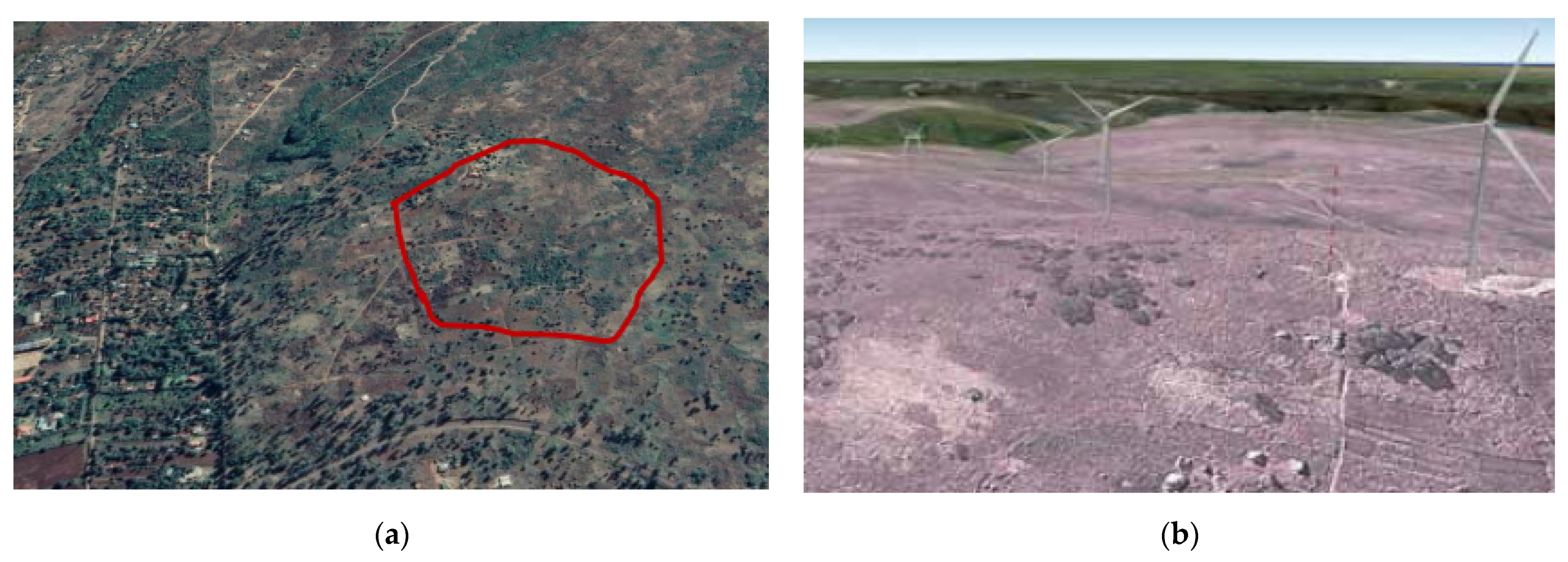
In many studies on Mozambique’s renewable power potential, Namaacha District has been singled out as one of the most prominent districts in terms of wind energy [32,33,34]. The district has a combination of reliefs from hills and mountains landscapes to plains and depressions landscapes and extensive lands favourable to the implementation of wind farms. Taking into account the weather conditions and landscape features in the Namaacha District, the National Energy Fund (FUNAE) held a mapping process and estimated the average wind speed and wind power generation potential of promising wind sites. Figure 2a represents the proposed wind site with an estimated area of 14.0 km2 (approximately 4.0 km wide and 3.5 km long), and Figure 2b illustrates the wind farm’s landscape area.
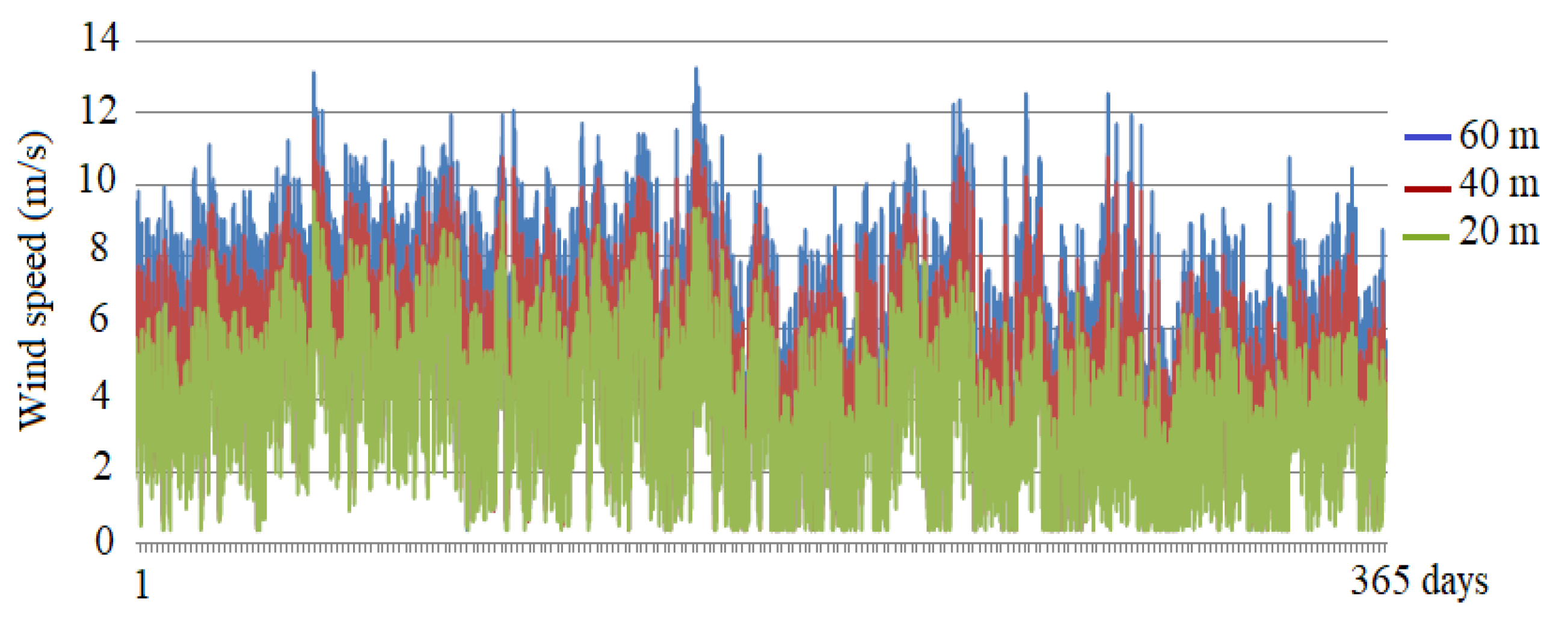
Three different wind farm layouts that differ in terms of distance between turbines, the row orientation angle, and spacing between rows were placed in the area, and the total energy production of the turbines was evaluated. In order to take full advantage of the Namaacha wind potential, FUNAE [32] recommends the installation of a wind tower with a height of about 60 m. Figure 3 shows the annual fluctuation of the wind speed with the height in Namaacha. As it is observed, the district´s average wind speed is estimated at 7.5 m/s.
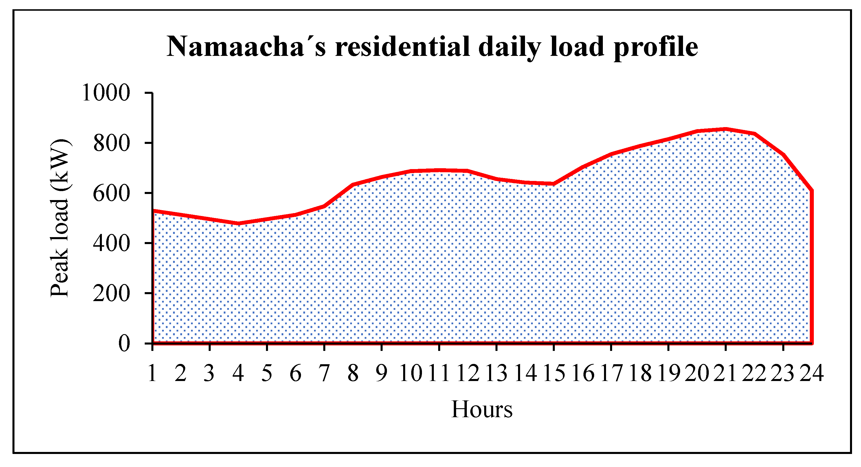
Although the daily load curve of the Namaacha power system has not changed its shape in the last years, there has been a considerable increase in terms of peak demand for electricity in the last decade. Figure 4 illustrates the typical daily load profile shape of the system.
4. Model Application and Assessment of Wake Effect on Turbine Performance
In this project, HOMER and SAM were used to size a wind system and to examine the wake effect on the farm. In HOMER, the determination of wind turbine power output entails three steps, namely, wind speed calculation at the hub height of the wind turbine, the estimation of power generated by the wind turbine at the wind speed standard air density, and finally, the adjustment of that power output value for the actual air density. The wind speed at the hub height of the wind turbine is calculated through the computing of the wind resource data provided. HOMER applies two distinct methods to estimate wind speed: the logarithm law and the power law. The first method is expressed as follows:
where
—is the wind speed at the hub height of the turbine [m/s];
—is the wind speed at the anemometer height [m/s];
—is the hub height of the turbine [m];
—is the anemometer height [m];
—is the surface roughness length [m].
By applying the second method, the wind speed at the hub height of the wind turbine is expressed as follows:
where
—is the wind speed at the hub height of the turbine [m/s];
—is the wind speed at the anemometer height [m/s];
—is the hub height of the wind turbine [m];
—is the anemometer height [m];
—is the power-law exponent.
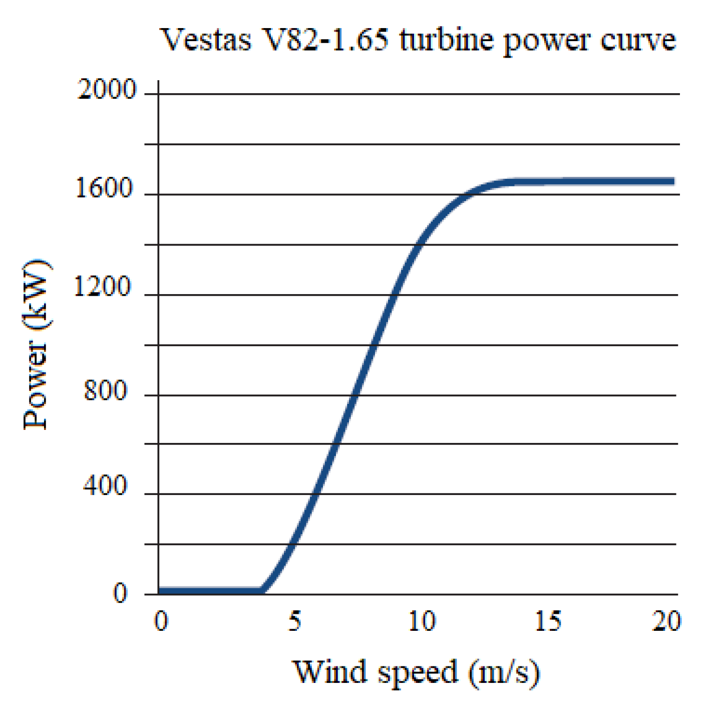
Once the hub height wind speed is calculated, with the help of the wind turbine power curve, the expected power of the wind turbine at this wind speed under normal temperature and pressure conditions is calculated. If the wind speed at the turbine hub height is not within the range defined in the power curve, the turbine will not generate power. Wind power technology fundaments the state that wind turbines will not produce power at wind speeds below the minimum cut-off or above the maximum cut-out wind speeds. Power curves typically specify wind turbine performance under normal temperature and pressure conditions.
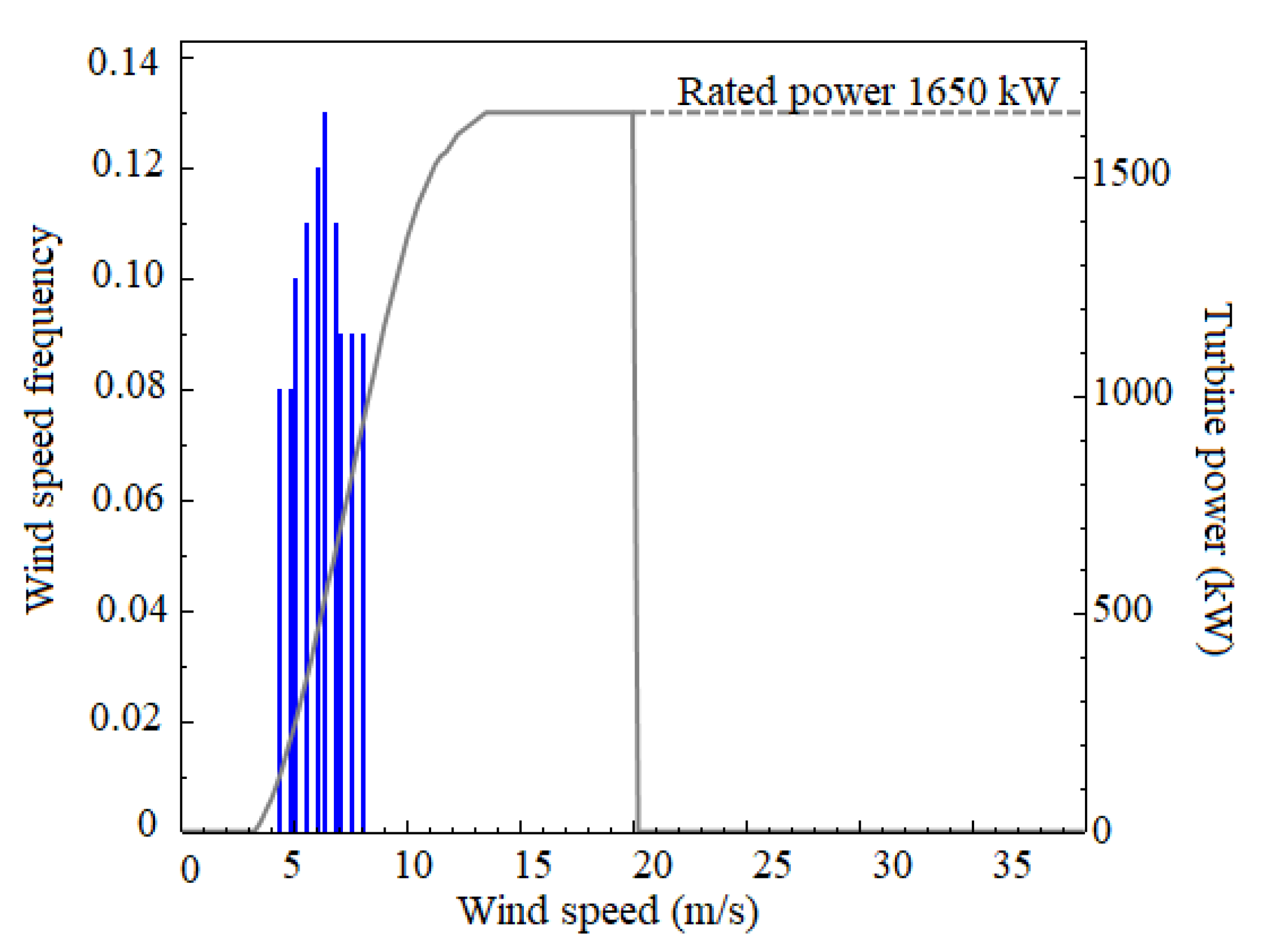
Figure 5 presents the power curve of the selected turbine Vestas V82-1.65 under varying wind conditions. Table 1 presents the turbine’s operating range of wind speed. According to Chaouachi et al. and Veena et al. [36,37], the selection of wind turbine follows three criteria: (1) reliability objective, which is related to the impact of the wind system on the electricity network security of supply; (2) the cost objective associated with the technology’s investment costs and the electricity tariff charged; (3) the performance, which is linked to the expected energy production and the correlation of wind profile patterns with corresponding load demand.
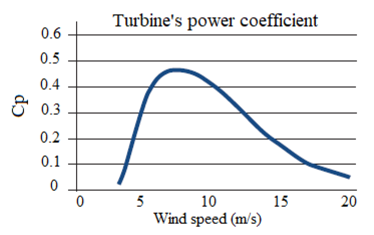
Taking into account the Namaacha wind profile, it is expected that the selected turbine will operate above its average power capacity for most of the year, with maximum production in periods of extreme wind speed. Regarding the efficiency of the turbine, it can be perceived from Figure 6 that the district’s wind speed profile allows the turbine to operate at its maximum power coefficient.
To adjust to real conditions, HOMER multiplies the power output predicted by the power curve by the air density ratio, according to the following equation:
where
—is the wind turbine power output [W];
—is the wind turbine power output at standard temperature and pressure conditions [W];
—is the actual air density [kg/m3];
—is the air density at standard temperature and pressure conditions [kg/m3].
In a real wind farm, the wind energy density experienced by individual wind turbines can differ significantly. In that context, the power output of a wind turbine may be affected by the wake effect of other wind turbines, and thus, in the design of wind farms, it is recommended to give an appropriate distance between two consecutive turbines to avoid disturbances in the performance of the downstream turbine [38]. Features of the wind farm that needs to be considered include fluctuations of wind speed, wind direction, and average wind speed [5]. Wind turbine farm models investigate the profile of the wind speed deficit downstream of the rotor that is captured by the subsequent turbine. A precise wake model is critical for the mathematical modelling of a wind farm and the optimal placement of wind turbines [27]. Considering the configuration of the wake, three types of models are presented: one-dimensional wake model, two-dimensional wake model, and three-dimensional wake model. The one-dimensional wake model is the well-known Jensen’s model, the two-dimensional wake model is the Gaussian variation of Jensen’s model, named Jensen–Gaussian model, and the three-dimensional wake model is the Gaussian wake model [27].
Given the thrust coefficient curve of the wind turbine and the wind farm design, the wake effect models can estimate the wake losses for each turbine. Apart from a reduction of the turbine’s power generated, the wake effect also leads to a dynamic load on the downstream turbine [25]. SAM presents three different wake effect methods to estimate the effect of upwind turbines in downwind turbine performance as follows:
- ▪
- Simple wake model—applies a thrust coefficient to calculate the wind speed deficit in each turbine due to the wake effect of the upwind turbines;
- ▪
- Wind resources assessment, siting, and energy model (WAsP model)—uses a decline constant to estimate the wind speed deficit behind each turbine and computes the overlap of that wake profile with the downwind turbine to calculate the wind speed at the downwind turbine;
- ▪
- Eddy–viscosity—is analogous to the WAsP model, and besides that, the wind speed shortage behind each turbine is presumed to have a Gaussian shape;
- ▪
- Constant loss—estimates wake loss as a constant percentage reduction in the wind farm output.
According to Shao et al. and Dhiman et al. [39,40], in the simple wake model, the wind speed in the wake is a function of the thrust coefficient (CT), and wake decline and is computed as follows:
where
—is the inflow velocity [m/s];
—is the thrust coefficient;
—is the downwind distance behind two consecutive wind turbines [m2];
—is the rotor radius [m];
—is the decay coefficient (φ = 0.075 for onshore wind farms) and (φ = 0.05 for offshore wind farms).
The difference in wind speed () between an upwind and downwind turbine is then
where
—is the thrust coefficient;
—is the downwind distance between two consecutive wind turbines [m];
—is the crosswind distance between two consecutive wind turbines [m];
—is the local turbulence coefficient estimated as .
In the WAsP method, the effective wind speed deficit at the downwind turbine is calculated using the following equation:
where
—is the inflow velocity [m/s];
—is the thrust coefficient;
—is the downwind distance behind two consecutive wind turbines [m2];
—is the rotor radius [m];
—is the decay coefficient (k = 0.075 for onshore wind farms) and (k = 0.05 for offshore wind farms);
—is the overlapped area of the swept area of the rotors;
—is the swept area of the upwind turbine’s rotor.
Regarding the Eddy–viscosity wake model which has a Gaussian shape, the studies in [25,27] present the following equation to estimate the wind velocity at the downstream wind turbine:
where
—is the thrust coefficient;
—is the rotor radius [m];
—is the downwind distance between two consecutive wind turbines [m];
—is the wake wide [m].
In this study, the investigation began with the calculation of wind farm capacity by applying HOMER. Considering the daily load profile of the Namaacha District provided by EDM [35], the wind speed profile provided by FUNAE [32], and investment costs per kW power of wind technology presented by IRENA [41,42] and Mazzeo et al. [43], HOMER sized the 33 MW wind farm for the district composed of 20 V82-1.65 MW turbines. Then, by introducing the turbine type and other input data in the SAM, the three distinct wind farm layouts were examined. The Eddy–viscosity model presented by SAM was applied considering the following losses evaluated by SAM: wake losses, availability losses, electrical losses, turbine performance losses, environmental losses, and operational strategies losses. These distinct categories of losses are expressed as a percentage of the total annual system output before losses and are defined to work in parallel with operating system uncertainties. Table 2 presents the assumed percentage of losses.
Losses effectively influence the optimal generation dispatch [44]. During the wind farm evaluation phase, environmental losses due to icing and other atmospheric conditions need to be assessed. The environmental losses estimation incorporates relatively great uncertainties due to the complexity of atmospheric phenomena. From Turkia et al. [45], environmental losses can vary from 4 to 17%. Namaacha does not experiment with severe atmospheric conditions, and therefore, environmental losses are considered to be 2.5%. Electrical losses in power systems are inevitable and occur due to the resistance of the current flowing in the circuit.
In wind farms, annual electrical losses range from 2 to 3% [46], and performance losses can reach 6% [47]. With the assumed losses, the wind farm’s wake losses were examined. Apart from the assumed losses, the wind farm layout was changed, and the effect of the losses on the system’s power output was optimised. The alteration in the layout of the wind farm was based on the arrangement of the erection of the turbines by modifying the distance between turbines and rows as well as the row orientation. With the change in orientation, the scattering of the turbines increases, and some turbines are not positioned behind the others. The desire of reducing the placement of the turbines one behind the other can also be achieved using the offset option of the rows.
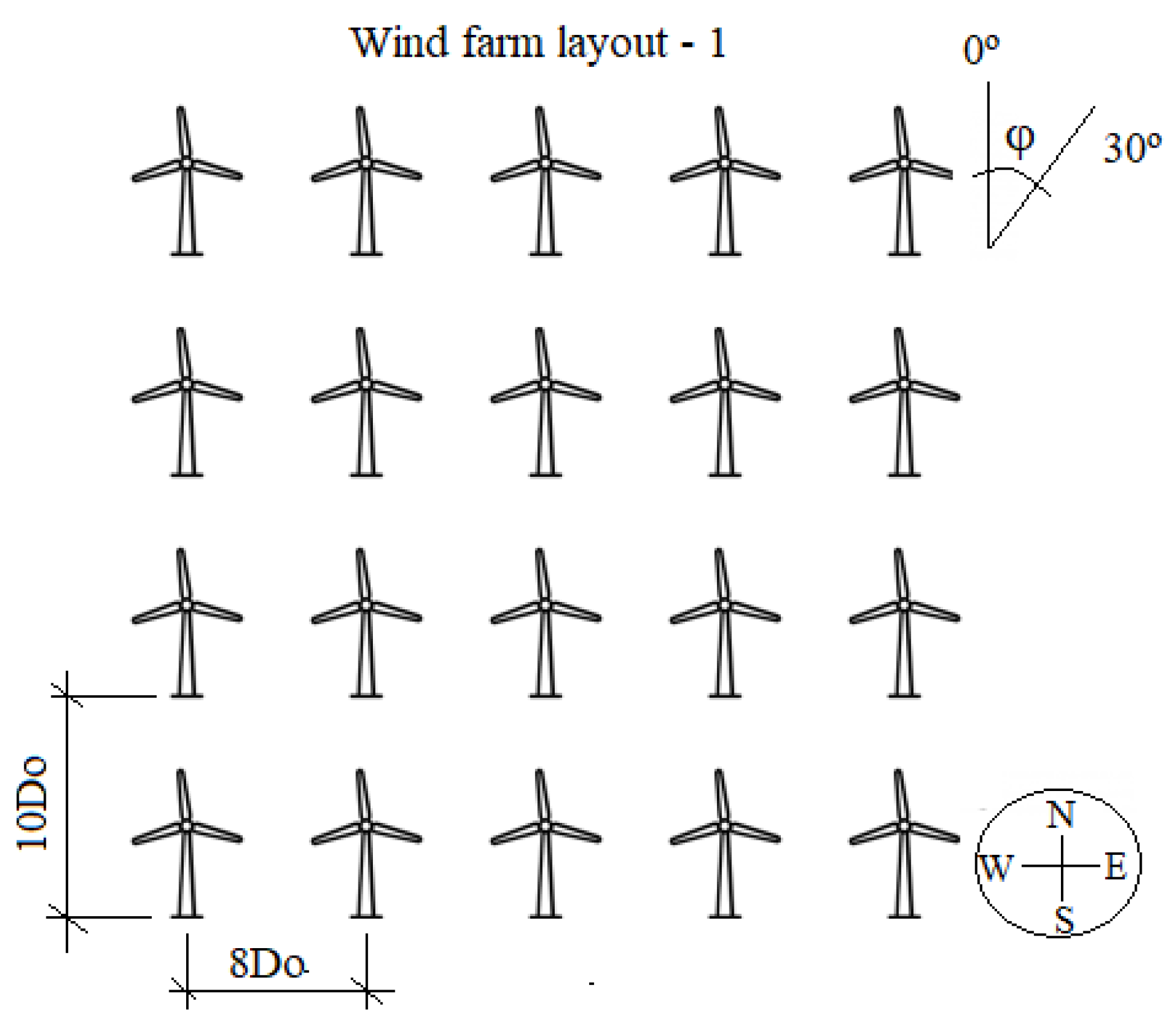
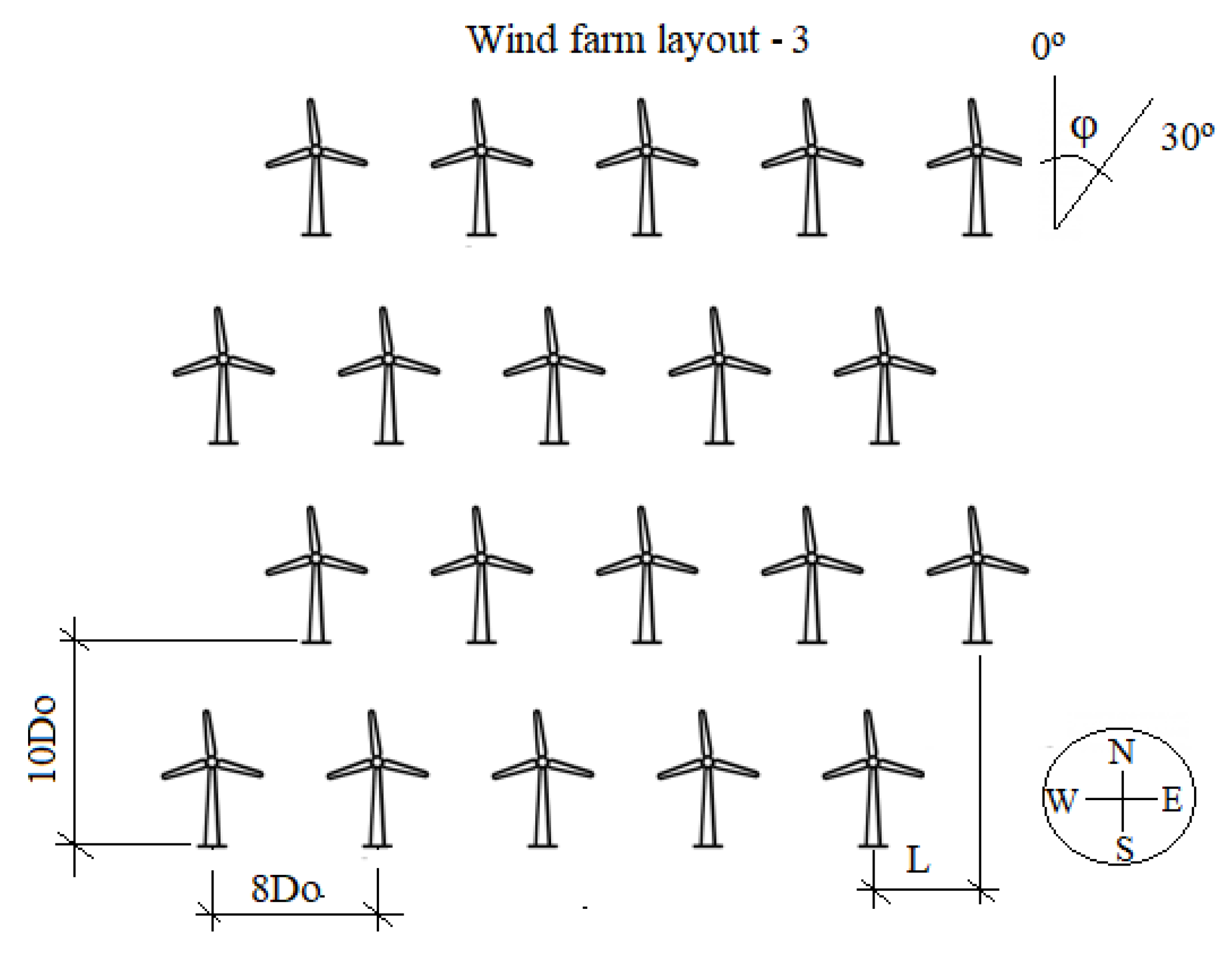
Figure 7 illustrates the primary design of the wind farm composed of 20 turbines; a major disturbance in the performance of the wind farm can occur in the downstream turbines. The primary distance between the turbines in each row and the spacing between rows was demarcated as a function of the rotor diameter Do. The row orientation was defined to be 0°, and thus, the lines are parallel to the equator. Regarding the offset of the rows, the value was set to L = 0 and the wind direction equal to φ = 0°.
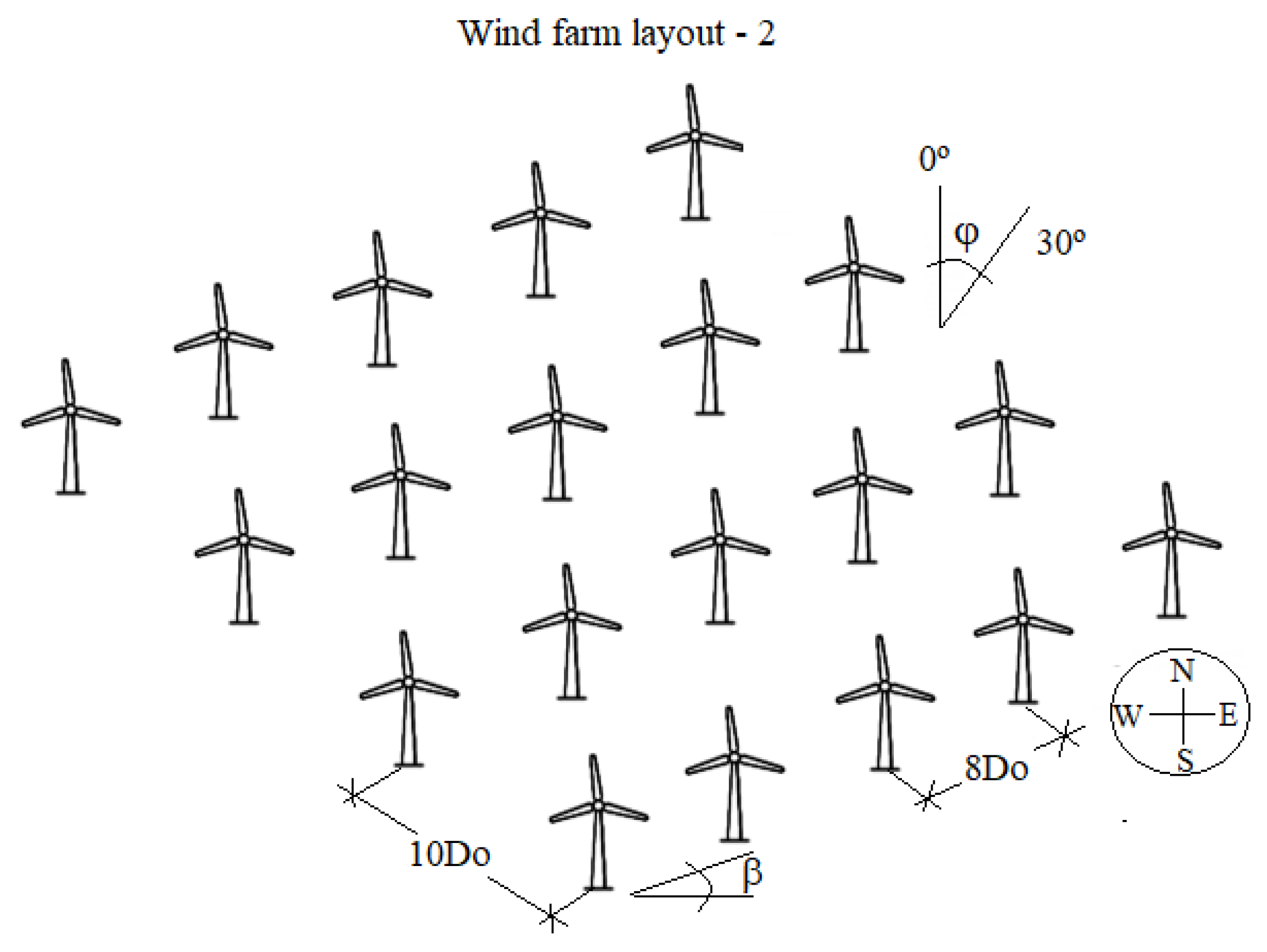
In Figure 8 and Figure 9, it can be observed that with the change in row orientation, the wind farm’s size increases. In a real wind farm, since wind direction continuously changes, the position of downstream turbines varies according to wind direction, and the wake effect in the wind farm also changes [48].
The wind speed in the farm was assumed to vary between 4.4 to 8 m/s; Figure 10 illustrates the distribution of the wind speed’s probability of occurrence. From Figure 6, it is observed that the V82-1.65 turbine presents better values of power for wind speed between 4 to 10 m/s.
In this study, the following three different wind farm layouts were analysed:
- ▪
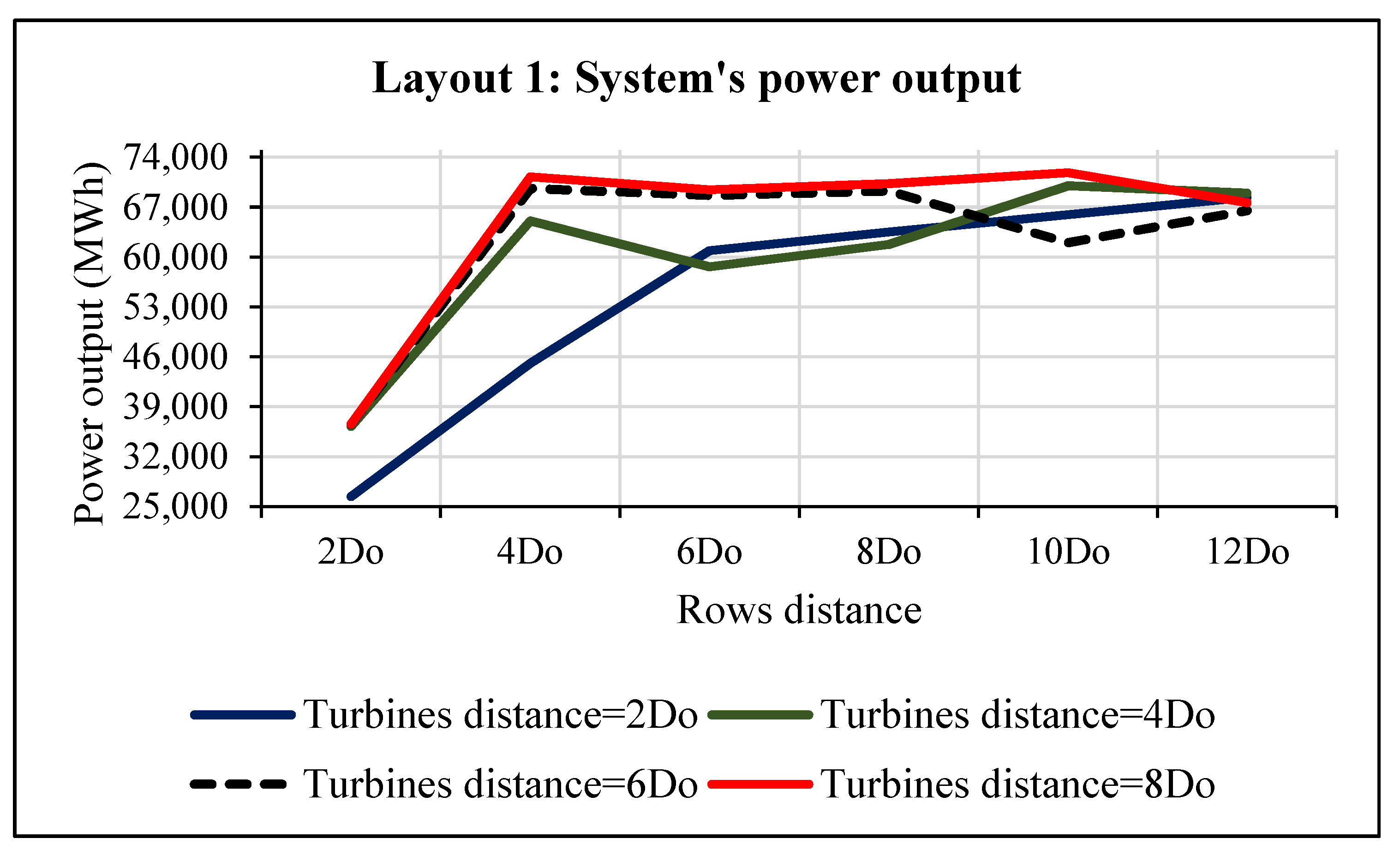
- Layout 1: examined the influence of the increased distance between turbines and the spacing between lines. The distances between turbines used were 2Do, 4Do, 6Do, and 8Do, while the spacing between rows used was 2Do, 4Do, 6Do, 8Do, 10Do, and 12Do. In this layout, in addition to varying the distance between turbines and lines, the wind direction varied from 0° to 60°. SAM considers wind direction equal to 0° when the wind blows from north to south. Row orientation angle and row offset was maintained as β = 0° and L = 0, respectively.
- ▪
- Layout 2: examined the influence of changing the row orientation angle. The following angles were used: 5°, 10°, 15°, 20°, 25°, and 30°. The optimal distance between the turbines and the rows, as well as the wind direction, was maintained at 8Do, 10Do, and 30°, respectively.
- ▪
- Layout 3: examined the influence of increased scattering of the turbines by changing the row offset. The following offset rows were used: 0, 0.5Do, Do 1.5Do, 2Do, 2.5Do, and 3Do. The optimal distance between the turbines and the rows, as well as the wind direction, was maintained at 8Do, 10Do, and 30°, respectively.
5. Results and Discussion
Taking into account the daily variation of energy consumption, the district’s wind energy potential, and costs of the wind technology, HOMER estimated that the necessary capacity of the wind farm is about 33 MW, comprising 20 V82-1.65 MW turbines. Given the thrust coefficient curve of the wind turbine and the wind farm design, wake effect models can estimate the wake losses in the wind farm. Apart from a reduction of turbines power generation, the wake effect also leads to a dynamic load on the downstream turbine [25].
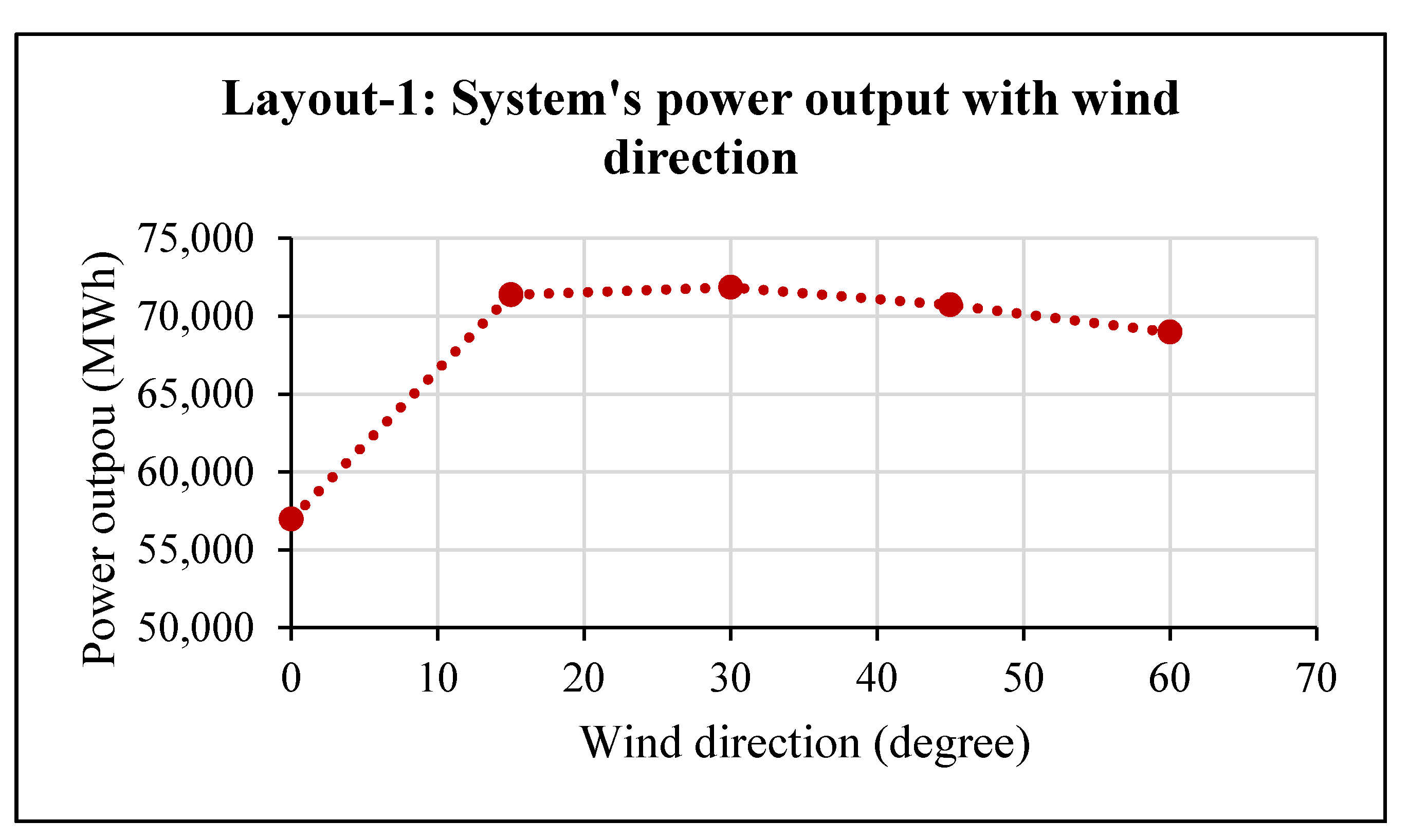
Figure 11 illustrates the wind site’s power generation according to the wind direction. When the wind direction is zero (from north to south), the disturbances in the air masses in the downstream turbines are more intense. Different from traditional energy resources, the wind resource has single features because of its temporal and seasonal variation. Therefore, wind power output technology fluctuates more strongly than traditional fossil fuel energy sources [16]. The change in wind direction creates temporary modifications in the wind farm layout and consequently the variation in power generation. From the analysis, it was observed that the highest rate of energy production occurs from a wind direction of 30°.
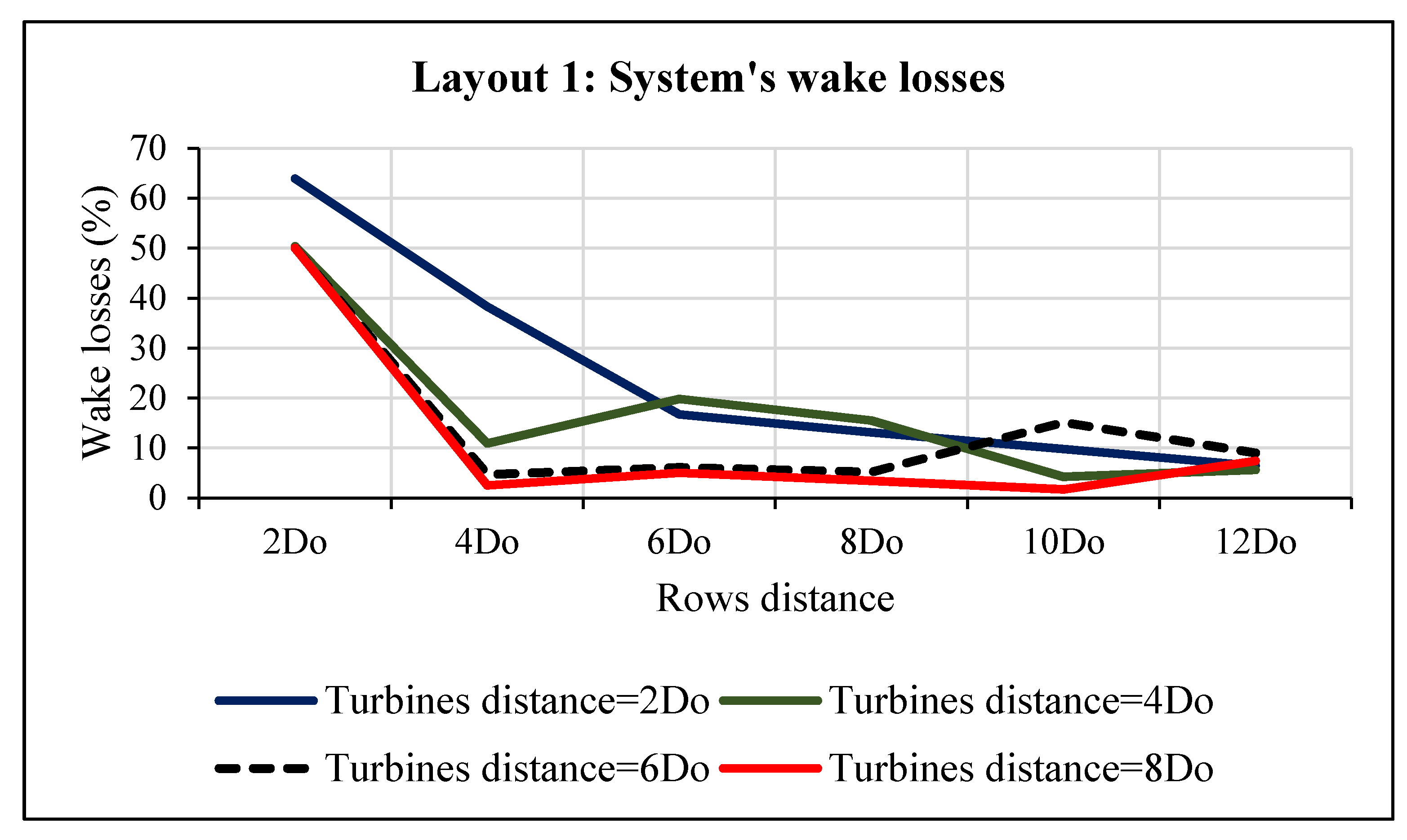
Taking into account the distance between the turbines and the lines assumed in layout 1 of the wind farm, Figure 12 and Figure 13 illustrate the system’s power output and wake losses, respectively. As can be perceived, by increasing the distance, the power can be improved and wake losses reduced, but an excessive increase in the distance between lines can cause a decline in power generation since, in a real wind farm, the decline in power generation is due to both the wake effect and the decrease of the wind mass load. On the other hand, although there is a marked gain in power generation and reduction of wake effect with the distance between turbines from 2Do to 4Do, in contrast to that, with the distance between turbines from 4Do to 8Do, the power generated remains practically constant.
For row spacing of 2Do and distance between turbines of 8Do, maximum wake loss is about 50%. A similar study [7] found a maximum wind deficit of approximately 45%, at a downstream distance of 2.5Do, and 35% at 3.5Do. Therefore, it is assumed that the optimal distance between turbines is 8Do, and the optimal spacing between rows is 10Do since this combination presents the highest energy production (71,844.0 MWh) and the lowest wake loss (1.7%). In terms of surface, layout 1 occupies approximately 6. 46 km2 (46.1%) of the available land.
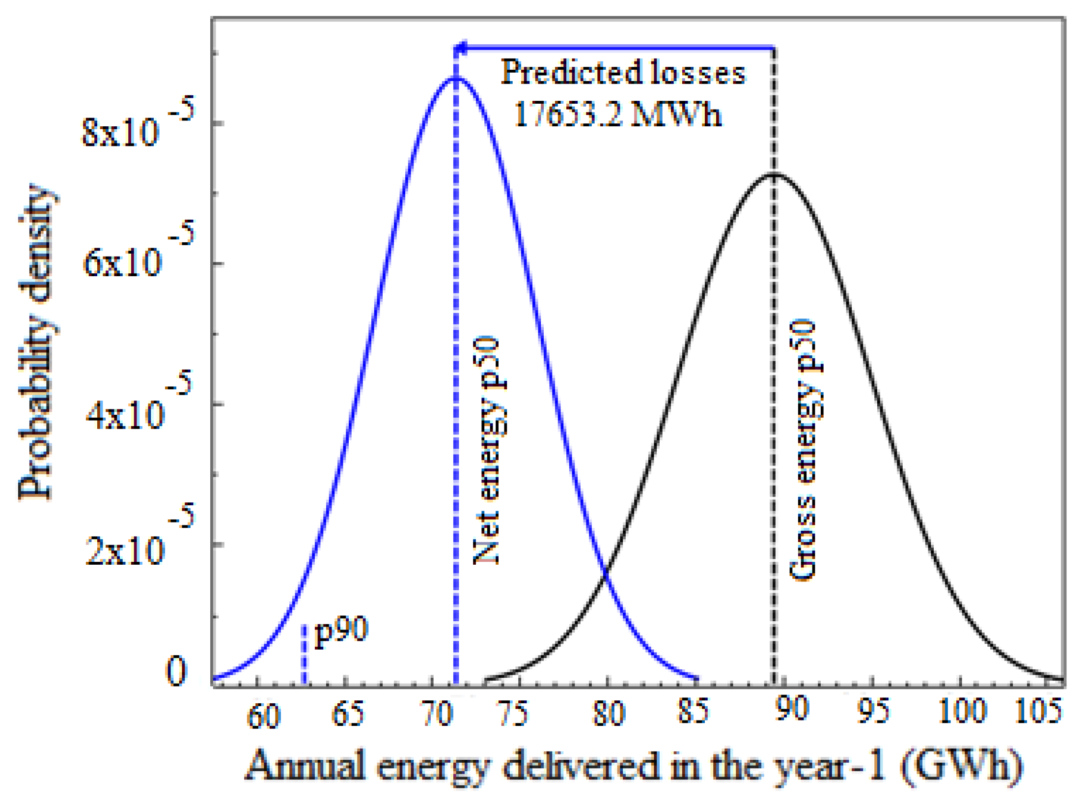
Taking into account all the variable assumed losses, Figure 14 specifies the probability density function of the annual energy delivered and estimates the predicted losses. In this layout, considering p50 probability, annual gross energy is about 89.49 GWh, and predicted losses are around 17,653.2 MWh.
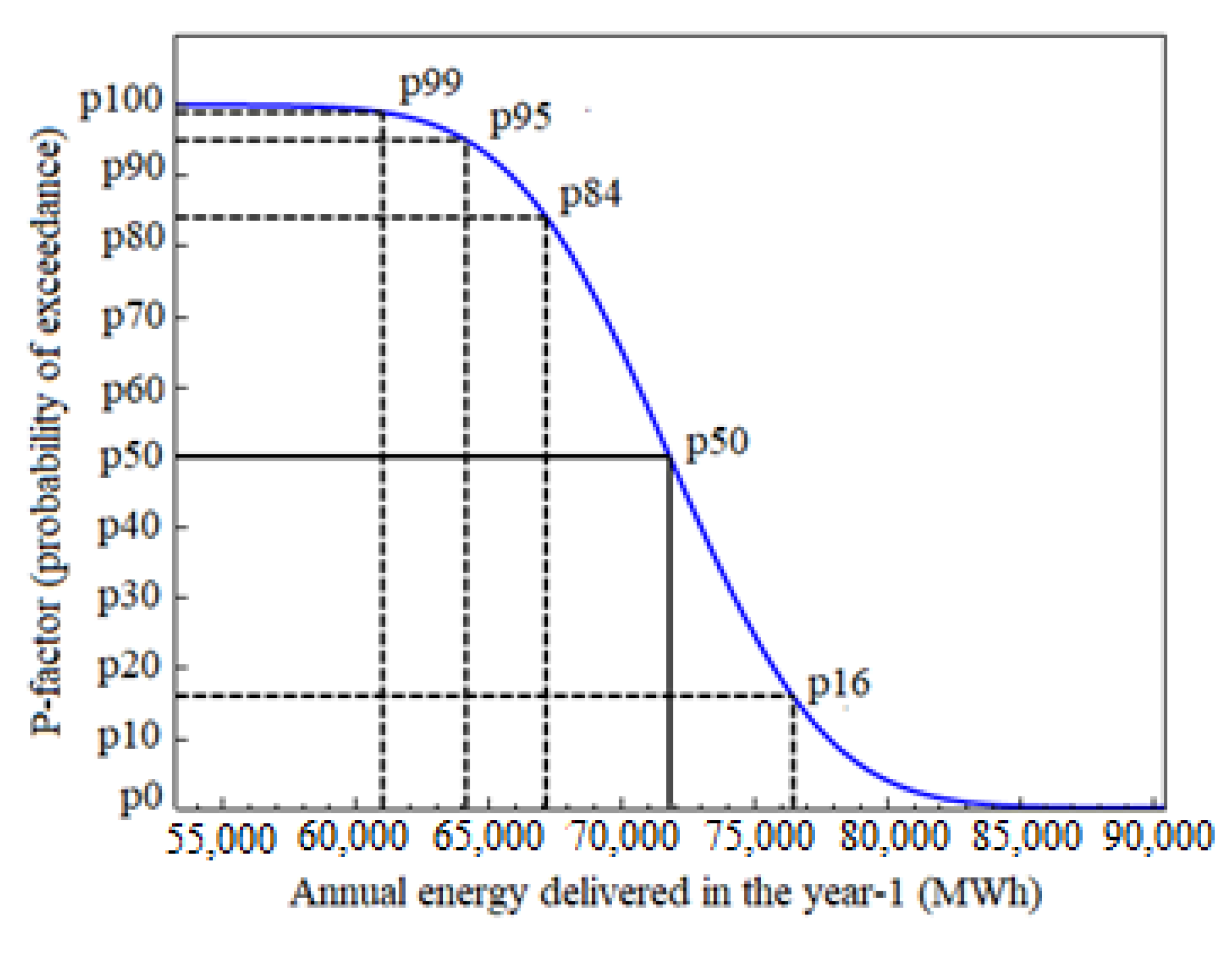
The performance of wind turbines is governed by both external conditions and turbine operation parameters, and thus, wind farm design uncertainties result in distinct factors such as wind speed measurement process, wake effects, terrain effects, extreme events, aerodynamics, and control [49]. Figure 15 displays year 1 probability distribution for the wind farm. In the wake losses analysis, the P50 energy production level is the mean energy production estimation, assuming a 50% probability of achieving annual power generation. A probability factor greater than 50, such as p95, represents more uncertainties presumed and therefore high predicted losses. On the contrary, probability factor minor than 50 such as p16 represents slight uncertainties presumed and therefore small predicted losses.
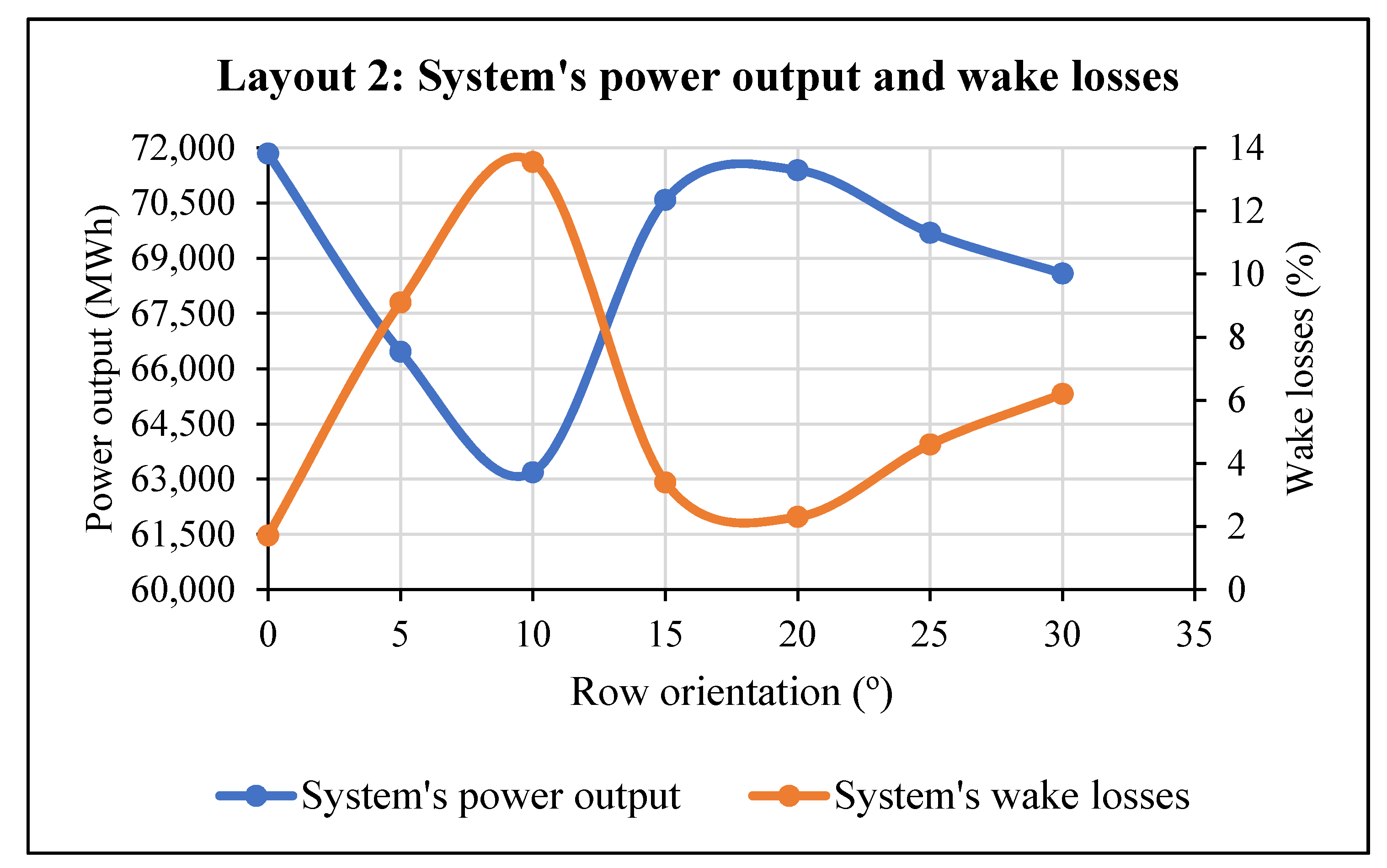
Figure 16 presents the fluctuation of the power output system and wake losses with row orientation. The analysis was performed to compare the wake losses in layout 1 and layout 2. From the analysis, it is observed that the minimum losses verified with modification of row orientation are of a higher magnitude than the minimum losses in layout 1. With rows orientation angle β = 0°, layout 1 predicted losses in the order of 1.7%, and with the variation of the row’s orientation, the angle β = 20° presented losses in the order of 2.3%.
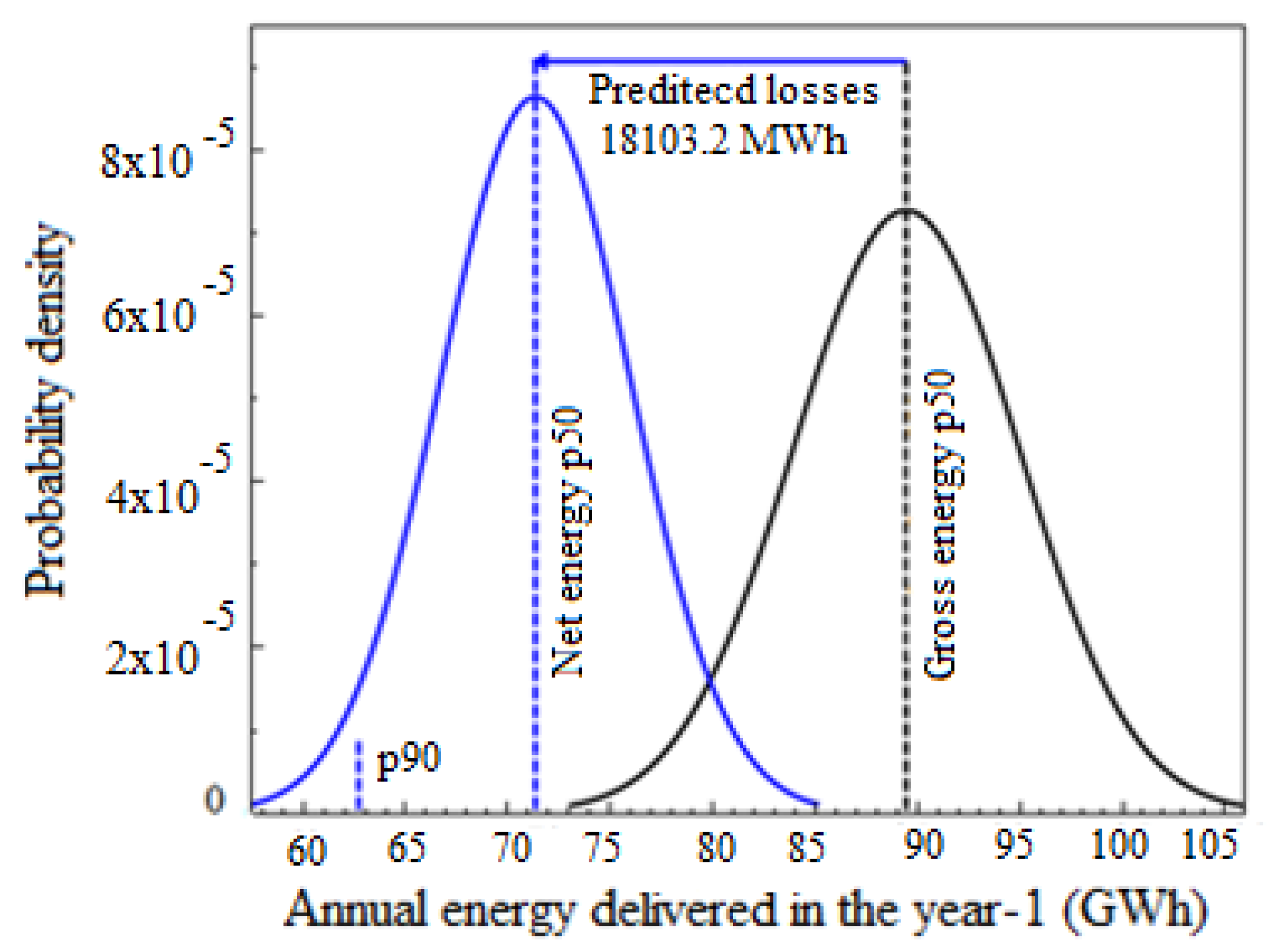
Taking into account all the assumed variables, layout 2 presented an annual predicted loss of about 18103.2 MWh (see Figure 17). In this layout, annual power production in year 1 is estimated as 71.39 GWh, and in terms of surface, layout 2 occupies approximately 11.12 km2 (79.4%) of the available land.
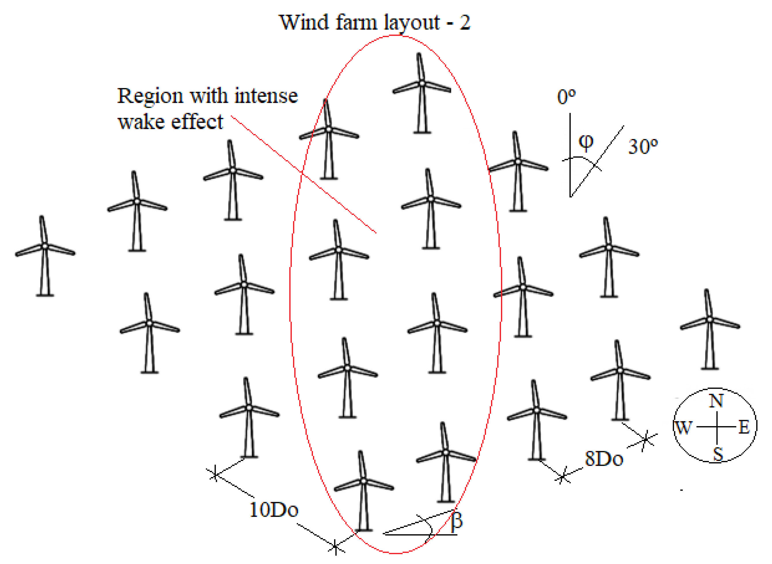
Wake losses in layout 2 are significant when the wind direction coincides with the direction comprising the largest number of turbines, as presented in Figure 18.
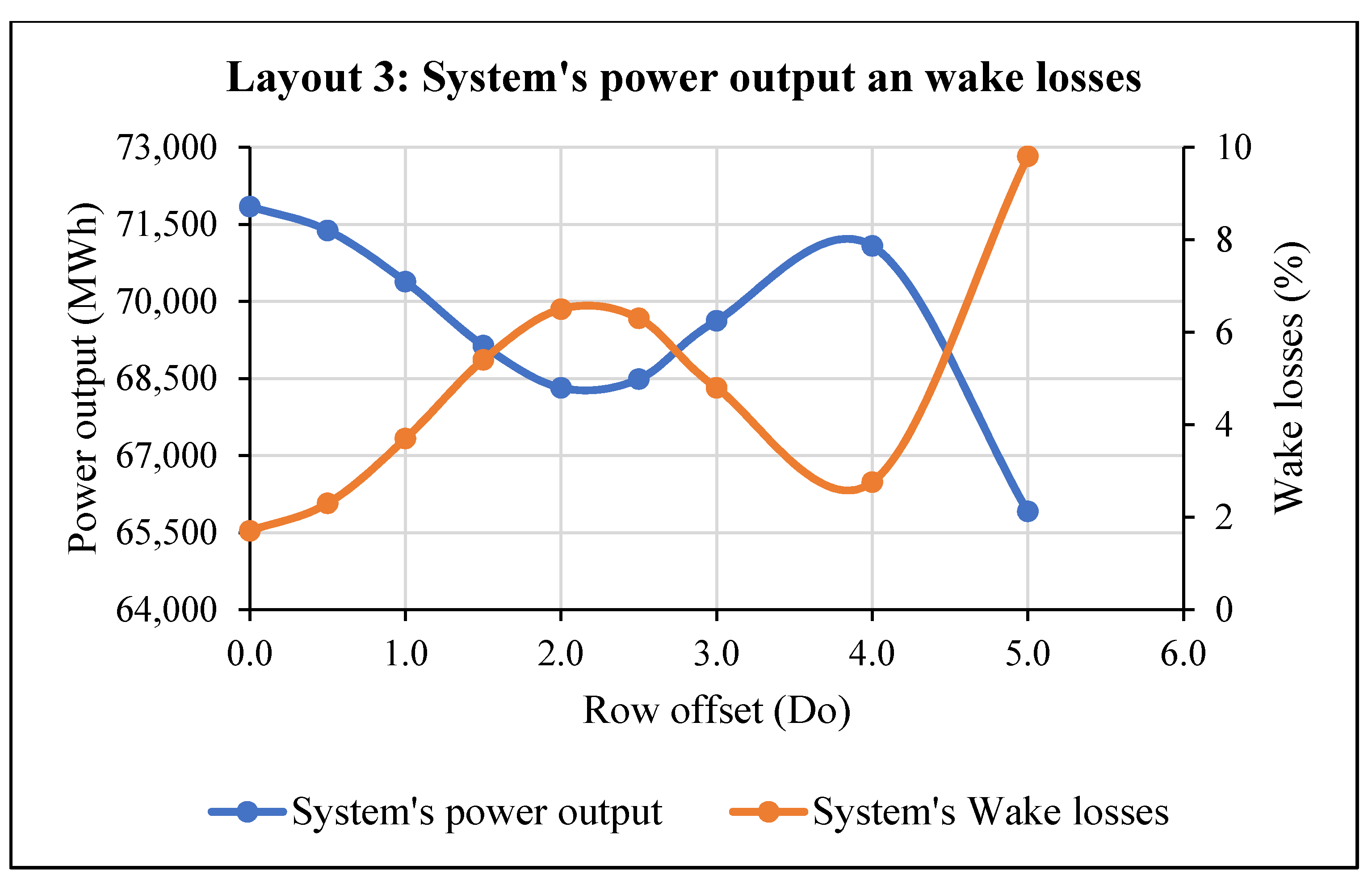
Regarding layout 3, Figure 19 displays the variation of the power output system and wake losses with row offset. The analysis aims to compare the system’s performance in layout 1 and layout 3. From the results, it is observed that the minimum losses verified with row offset are of a higher magnitude than the minimum losses in layout 1 with rows offset L = 0. Applying the strategy of row offset, the minimum losses are achieved with L = 0.5Do and represent 2.3%. However, this percentage is above the minimal losses obtained in layout 1. In terms of surface, layout 3 occupies approximately 6.82 km2 (48.7%) of the available land.
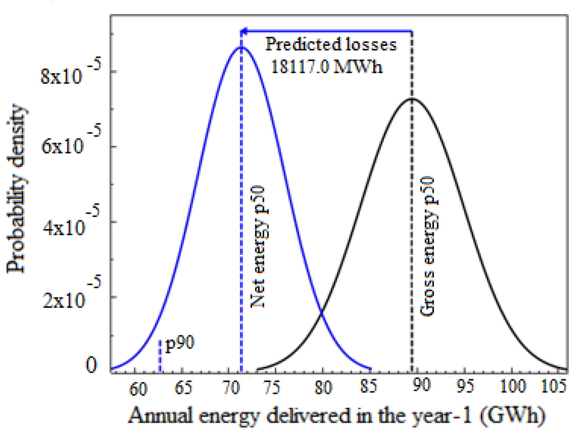
Considering the variable assumed, layout 3 presented an annual predicted loss of about 18,117.0 MWh, as illustrated in Figure 20. In this layout, annual power production in year 1 is estimated as 71.37 GWh.
6. Conclusions
The study investigated the wake effect in the wind farm in the District of Namaacha due to the wind farm’s layout. Considering the constraint of land availability, three different dispositions of the turbines in the wind farm were studied in order to find out the placement that would minimise wake losses with efficient utilisation of land. From the results, it was concluded that the influence of the wake effect is unpredictable but can be minimised with an adequate disposition of the turbines and optimal distancing. Regarding the spacing between turbines, layout 1 demonstrated that the optimal distance between turbines is about 8Do and the optimal distance between rows is around 10Do. The examination of the longitudinal distance between the turbines showed that the wake effect begins to decline from 4Do, and the tendency continues until 10Do. After 10Do, the energy losses due to the wake effect begin to increase again. In relation to the transversal distance between the turbines, the wake effect would start to reduce from 6Do, but the optimal transversal distance being about 8Do. The increment of the transversal distance above 8Do brings a slight gain of power production associated with high use of land, and therefore, it is not recommended. It is noted that layout 1, compared with layout 2, shows a minor percentage of loss (1.7%) and also lower use of available land (46%). In layout 2, due to the rotation of the rows, in the diagonal line of the wind farm, the wind mass crosses a greater number of turbines, and consequently, there is an increase in power losses as a result of the wake effect. The wake losses in layout 2 are around 2.3%, and therefore, the study proves that in real wind farms, when the wind direction coincides with the line comprising the largest number of turbines, wake losses can be significant, and this usually occurs in the diagonal lines of the wind farm. On the other hand, in the diagonal line, in addition to the superior number of turbines, the spacing between two consecutive turbines exceeds the optimum distance of 10Do, and thus, in addition to the increase in losses, there is an inefficient use of land. With respect to the comparison between layout 1 and layout 3, the results emphasise the robustness of layout 1, since the layout continues to present minor wake losses and percentage of used land. Note that layout 3 presents losses in the order of 2.3%, as well as layout 2, but land occupation is 48.7%. However, in terms of preference between layout 2 and layout 3, the last one presents less land occupation which is an advantage.
Author Contributions
Conceptualisation, P.M.J.R., S.P.C. and Z.H.; Methodology, P.M.J.R. and S.P.C.; Validation, P.M.J.R., S.P.C. and Z.H.; formal analysis, P.M.J.R., S.P.C. and Z.H.; investigation, P.M.J.R., S.P.C. and Z.H.; resources, P.M.J.R.; data curation, P.M.J.R., S.P.C. and Z.H.; writing—original draft preparation, P.M.J.R. and S.P.C.; writing—review and editing, P.M.J.R., S.P.C. and Z.H.; visualisation, P.M.J.R., S.P.C. and Z.H. All authors have read and agreed to the published version of the manuscript.
Funding
This research received no external funding.
Informed Consent Statement
The authors hereby agree to publish this paper as Co-Authors in the sequence of Names as above on the basis of our (1) contributions and participations in formulating the research problem, or analysing and interpreting the data or have made other substantial scholarly effort or a combination of these; and/or (2) participations in writing the paper; and (3) approvals of the final version for publication and preparedness to defend the publication against criticisms.
Data Availability Statement
Data collected from FUNAE, Mozambique with permission.
Acknowledgments
The authors would like to acknowledge the Tshwane University of Technology, Departments of Electrical and Mechanical and Mechatronics Engineering, Pretoria, South Africa, for all the conditions provided in order to conduct the research and writing of this paper.
Conflicts of Interest
The authors declare no conflict of interest.
Nomenclature
| Upstream wind speed approaching the turbine [m/s] | |
| Wind speed at the rotor [m/s] | |
| Downstream wind speed [m/s] | |
| Air mass flow rate [kg/s] | |
| Force on the turbine resulting from the air mass flow [N] | |
| Power extracted by the turbine [W] | |
| Energy extracted from the wind [W] | |
| Air density [kg/m3] | |
| Swept area of the blades [m2] | |
| Overlapped area of the swept area of the rotors [m2] | |
| Interference factor | |
| Power of the undisturbed upstream air mass | |
| Power coefficient | |
| Shape factor | |
| Scale factor | |
| Wind speed at the hub height of the turbine [m/s] | |
| Wind speed at the anemometer height [m/s] | |
| Hub height of the turbine [m] | |
| Anemometer height [m] | |
| Surface roughness length [m] | |
| Power law exponent | |
| Turbine power output at standard temperature and pressure conditions [W] | |
| Air density at standard temperature and pressure conditions [kg/m3] | |
| Thrust coefficient | |
| Rotor radius [m] | |
| Decay coefficient | |
| Downwind distance between two consecutive wind turbines [m] | |
| Crosswind distance between two consecutive wind turbines [m] | |
| Local turbulence coefficient | |
| Wake wide [m] | |
| Wind direction [°] | |
| Turbines row orientation angle [°] | |
| Rotor diameter [m] | |
| Row offset distance [m] |
References
- Moussa, M.O. Experimental and numerical performances analysis of a small three blades wind turbine. Energy 2020, 203, 117807. [Google Scholar] [CrossRef]
- Wilkie, D.; Galasso, C. Impact of climate-change scenarios on offshore wind turbine structural performance. Renew. Sustain. Energy Rev. 2020, 134, 110323. [Google Scholar] [CrossRef]
- Nazir, M.S.; Alturise, F.; Alshmrany, S.; Nazir, H.M.J.; Bilal, M.; Abdalla, A.N.; Sanjeevikumar, P.; Ali, Z.M. Wind generation forecasting methods and proliferation of artificial neural network: A review of five years research trend. Sustainability 2020, 12, 3778. [Google Scholar] [CrossRef]
- Ulazia, A.; Ibarra-Berastegi, G.; Sáenz, J.; Carreno-Madinabeitia, S.; González-Rojí, S.J. Seasonal Correction of Offshore Wind Energy Potential due to Air Density: Case of the Iberian Peninsula. Sustainability 2019, 11, 3648. [Google Scholar] [CrossRef] [Green Version]
- Guo, P.; Chen, S.; Chu, J.; Infield, D. Wind direction fluctuation analysis for wind turbines. Renew. Energy 2020, 162, 1026–1035. [Google Scholar] [CrossRef]
- Urabe, C.T.; Saitou, T.; Kataoka, K.; Ikegami, T.; Ogimoto, K. Positive Correlations between Short-Term and Average Long-Term Fluctuations in Wind Power Output. Energies 2021, 14, 1861. [Google Scholar] [CrossRef]
- Sun, H.; Gao, X.; Yang, H. A review of full-scale wind-field measurements of the wind-turbine wake effect and a measurement of the wake-interaction effect. Renew. Sustain. Energy Rev. 2020, 132, 110042. [Google Scholar] [CrossRef]
- Veludurthi, A.; Bolleddu, V. Experimental buckling analysis of NACA 63415 aerofoil wind turbine blade. Mater. Today Proc. 2021, 46, 205–211. [Google Scholar] [CrossRef]
- Rahgozar, S.; Pourrajabian, A.; Kazmi, S.A.A. Performance analysis of a small horizontal axis wind turbine under the use of linear/nonlinear distributions for the chord and twist angle. Energy Sustain. Dev. 2020, 58, 42–49. [Google Scholar] [CrossRef]
- Fant, C.; Gunturu, B.; Schlosser, A. Characterizing wind power resource reliability in southern Africa. Appl. Energy 2016, 161, 565–573. [Google Scholar] [CrossRef] [Green Version]
- Jin, G.; Zong, Z.; Jiang, Y.; Zou, L. Aerodynamic analysis of side-by-side placed twin vertical-axis wind turbines. Ocean Eng. 2020, 209, 107296. [Google Scholar] [CrossRef]
- Leelakrishnan, E.; Kumar, M.S.; Selvaraj, S.D.; Vignesh, N.S.; Raja, T.A. Numerical evaluation of optimum tip speed ratio for darrieus type vertical axis wind turbine. Mater. Today Proc. 2020, 33, 4719–4722. [Google Scholar] [CrossRef]
- Vergaerde, A.; De Troyer, T.; Muggiasca, S.; Bayati, I.; Belloli, M.; Kluczewska-Bordier, J.; Parneix, N.; Silvert, F.; Runacres, M.C. Experimental characterisation of the wake behind paired vertical-axis wind turbines. J. Wind. Eng. Ind. Aerodyn. 2020, 206, 104353. [Google Scholar] [CrossRef]
- Boudounit, H.; Tarfaoui, M.; Saifaoui, D. Modal analysis for optimal design of offshore wind turbine blades. Mater. Today Proc. 2020, 30, 998–1004. [Google Scholar] [CrossRef]
- Ouammi, A.; Dagdougui, H.; Sacile, R.; Mimet, A. Monthly and seasonal assessment of wind energy characteristics at four monitored locations in Liguria region (Italy). Renew. Sustain. Energy Rev. 2010, 14, 1959–1968. [Google Scholar] [CrossRef]
- Feroz, R.M.A.; Javed, A.; Syed, A.H.; Kazmi, S.A.A.; Uddin, E. Wind speed and power forecasting of a utility-scale wind farm with inter-farm wake interference and seasonal variation. Sustain. Energy Technol. Assess. 2020, 42, 100882. [Google Scholar] [CrossRef]
- Longo, R.; Nicastro, P.; Natalini, M.; Schito, P.; Mereu, R.; Parente, A. Impact of urban environment on Savonius wind turbine performance: A numerical perspective. Renew. Energy 2020, 156, 407–422. [Google Scholar] [CrossRef]
- Regodeseves, P.G.; Morros, C.S. Unsteady numerical investigation of the full geometry of a horizontal axis wind turbine: Flow through the rotor and wake. Energy 2020, 202, 117674. [Google Scholar] [CrossRef]
- Ali, Q.S.; Kim, M.H. Unsteady aerodynamic performance analysis of an airborne wind turbine under load varying conditions at high altitude. Energy Convers. Manag. 2020, 210, 112696. [Google Scholar] [CrossRef]
- Hohman, T.; Martinelli, L.; Smits, A. The effect of blade geometry on the structure of vertical axis wind turbine wakes. J. Wind. Eng. Ind. Aerodyn. 2020, 207, 104328. [Google Scholar] [CrossRef]
- Pallotta, A.; Pietrogiacomi, D.; Romano, G. HYBRI—A combined Savonius-Darrieus wind turbine: Performances and flow fields. Energy 2020, 191, 116433. [Google Scholar] [CrossRef]
- Wang, Z.; Wang, S.; Ren, J.; Meng, X.; Wu, Y. Model experiment study for ventilation performance improvement of the Wind Energy Fan system by optimizing wind turbines. Sustain. Cities Soc. 2020, 60, 102212. [Google Scholar] [CrossRef]
- Fei, Z.; Tengyuan, W.; Xiaoxia, G.; Haiying, S.; Hongxing, Y.; Zhonghe, H.; Yu, W.; Xiaoxun, Z. Experimental study on wake interactions and performance of the turbines with different rotor-diameters in adjacent area of large-scale wind farm. Energy 2020, 199, 117416. [Google Scholar] [CrossRef]
- Abraham, A.; Hong, J. Dynamic wake modulation induced by utility-scale wind turbine operation. Appl. Energy 2020, 257, 114003. [Google Scholar] [CrossRef]
- Dhiman, H.S.; Deb, D.; Foley, A.M. Bilateral Gaussian Wake Model Formulation for Wind Farms: A Forecasting Based Approach. Renew. Sustain. Energy Rev. 2020, 127, 109873. [Google Scholar] [CrossRef]
- Ge, M.; Zhang, S.; Meng, H.; Ma, H. Study on interaction between the wind-turbine wake and the urban district model by large eddy simulation. Renew. Energy 2020, 157, 941–950. [Google Scholar] [CrossRef]
- Tao, S.; Xu, Q.; Feijóo, A.; Zheng, G.; Zhou, J. Wind farm layout optimization with a three-dimensional Gaussian wake model. Renew. Energy 2020, 159, 553–569. [Google Scholar] [CrossRef]
- Saad, A.S.; El-Sharkawy, I.I.; Ookawara, S.; Ahmed, M. Performance enhancement of twisted-bladed Savonius vertical axis wind turbines. Energy Convers. Manag. 2020, 209, 112673. [Google Scholar] [CrossRef]
- Dorel, S.F.; Mihai, G.A.; Nicusor, D. Review of Specific Performance Parameters of Vertical Wind Turbine Rotors Based on the SAVONIUS Type. Energies 2021, 14, 1962. [Google Scholar] [CrossRef]
- Sedighi, H.; Akbarzadeh, P.; Salavatipour, A. Aerodynamic performance enhancement of horizontal axis wind turbines by dimples on blades: Numerical investigation. Energy 2020, 195, 117056. [Google Scholar] [CrossRef]
- Twidell, J.; Weir, T. Renewable Energy Resources, 2nd ed.; Renewable Energy Resources in ASEAN; Taylor and Francis: 2018. pp. 4–10. Available online: http://www.uobabylon.edu.iq/eprints/publication_4_10679_78.pdf (accessed on 14 July 2020).
- Fundo Nacional de Energia. Renewable Energy Atlas of Mozambique; Gesto Energia S.A.: Maputo, Mozambique, 2014. [Google Scholar]
- Minister of Energy Mozambique, Riso National Laboratoty-Denmark. Support for Wind Power Development in Mozambique Final Report (Draft) June 2008; DNER Risø Danida: Copenhagen, Denmark, 2008. [Google Scholar]
- Mokveld, K.; von Eije, S. Final Energy Report Mozambique; Netherlands Enterprise Agency: Assen, The Netherlands, 2018; pp. 1–43. [Google Scholar]
- EDM. Annual Statistical Report 2016; EDM: Maputo, Mozambique, 2016. [Google Scholar]
- Chaouachi, A.; Covrig, C.F.; Ardelean, M. Multi-criteria selection of offshore wind farms: Case study for the Baltic States. Energy Policy 2017, 103, 179–192. [Google Scholar] [CrossRef]
- Veena, R.; Manuel, S.; Mathew, S.; Petra, I. Parametric Models for Predicting the Performance of Wind Turbines. Mater. Today Proc. 2020, 24, 1795–1803. [Google Scholar] [CrossRef]
- Sun, H.; Yang, H. Numerical investigation of the average wind speed of a single wind turbine and development of a novel three-dimensional multiple wind turbine wake model. Renew. Energy 2020, 147, 192–203. [Google Scholar] [CrossRef]
- Shao, Z.; Wu, Y.; Li, L.; Han, S.; Liu, Y. Multiple Wind Turbine Wakes Modeling Considering the Faster Wake Recovery in Overlapped Wakes. Energies 2019, 12, 680. [Google Scholar] [CrossRef] [Green Version]
- Dhiman, H.S.; Deb, D.; Balas, V.E. Supervised learning for forecasting in presence of wind wakes. In Supervised Machine Learning in Wind Forecasting and Ramp Event Prediction; Academic Press: Cambridge, MA, USA, 2020; pp. 141–169. [Google Scholar]
- International Renewable Energy Agency. Renewable Power Generation Costs in 2017; IRENA: Abu Dhabi, United Arab Emirates, 2018. [Google Scholar]
- International Renewable Energy Agency. Electricity Storage and Renewables: Costs and Markets to 2030; IRENA: Abu Dhabi, United Arab Emirates, 2017. [Google Scholar]
- DMazzeo, D.; Baglivo, C.; Matera, N.; De Luca, P.; Congedo, P.M.; Oliveti, G. Energy and economic dataset of the worldwide optimal photovoltaic-wind hybrid renewable energy systems. Data Brief 2020, 33, 106476. [Google Scholar] [CrossRef]
- Farahmand, H.; Warland, L.; Huertas-Hernando, D. The Impact of Active Power Losses on the Wind Energy Exploitation of the North Sea. Energy Procedia 2014, 53, 70–85. [Google Scholar] [CrossRef] [Green Version]
- Turkia, V.; Huttunen, S.; Wallenius, T. Method for Estimating Wind Turbine Production Losses due to Icing; VTT Technical Research Centre of Finland: Espoo, Finland, 2013. [Google Scholar]
- Colmenar-Santos, A.; Campíñez-Romero, S.; Enríquez-Garcia, L.A.; Pérez-Molina, C. Simplified analysis of the electric power losses for on-shore wind farms considering weibull distribution parameters. Energies 2014, 7, 6856–6885. [Google Scholar] [CrossRef] [Green Version]
- Byrne, R.; Astolfi, D.; Castellani, F.; Hewitt, N.J. A Study of Wind Turbine Performance Decline with Age through Operation Data Analysis. Energies 2020, 13, 2086. [Google Scholar] [CrossRef] [Green Version]
- Ge, X.; Chen, Q.; Fu, Y.; Chung, C.Y.; Mi, Y. Optimization of maintenance scheduling for offshore wind turbines considering the wake effect of arbitrary wind direction. Electr. Power Syst. Res. 2020, 184, 106298. [Google Scholar] [CrossRef]
- Premkumar, P.S.; Nadaraja P., S.; Arunvinthan, S.; Sivaraja, S.; Vinayagamurthy, G.V.; Peradotto, E.; Panunzio, A.M.; Salles, L.; Schwingshackl, C.; Bacharoudis, K.C.; et al. Uncertainty and Risk Assessment in the Design Process for Wind. J. Adv. Res. Dyn. Control Syst. 2015, 9, V07AT30A013. [Google Scholar]
Figure 1.
Representation of upwind and downwind stream for wind turbines.

Figure 2.
(a) Proposed site for Namaacha wind farm. Courtesy of Google Earth, land for wind farm allocation (25°58′19″ S, 32°01′56″ E, elevation 497M); (b) Overview of the wind farm’s landscape. Courtesy of FUNAE [32].
Figure 2.
(a) Proposed site for Namaacha wind farm. Courtesy of Google Earth, land for wind farm allocation (25°58′19″ S, 32°01′56″ E, elevation 497M); (b) Overview of the wind farm’s landscape. Courtesy of FUNAE [32].

Figure 3.
Namaacha’s annual wind speed profile. Courtesy of FUNAE [32].
Figure 3.
Namaacha’s annual wind speed profile. Courtesy of FUNAE [32].

Figure 4.
Namaacha′s typical residential daily load profile on 15 January. Courtesy of Mozambique Power Company (EDM) [35].
Figure 4.
Namaacha′s typical residential daily load profile on 15 January. Courtesy of Mozambique Power Company (EDM) [35].

Figure 5.
Vestas V82-1.65 turbine power curve. Courtesy of Vestas Wind System.

Figure 6.
Vestas V82-1.65 turbine power curve. Courtesy Vestas Wind System.

Figure 7.
Optimal wind farm (layout 1) with the distance between turbines equal to 8D0, the distance between rows equal to 10D0, and wind direction angle equal to 30°.
Figure 7.
Optimal wind farm (layout 1) with the distance between turbines equal to 8D0, the distance between rows equal to 10D0, and wind direction angle equal to 30°.

Figure 8.
Modified wind farm (layout 2), considering row orientation angle.

Figure 9.
Modified wind farm (layout 3) considering row offset.

Figure 10.
Distribution of the wind speed’s probability of occurrence.

Figure 11.
System’s power output for different wind directions.

Figure 12.
System’s power output for different distances between turbines and rows.

Figure 13.
System’s wake losses for different distances between turbines and rows.

Figure 14.
System’s predicted losses considering wake losses (layout 1).

Figure 15.
System’s P16, P50, P84, P95, P99 probability of annual energy production (layout 1).

Figure 16.
System’s power output for different rows orientation angles.

Figure 17.
System’s predicted losses considering wake losses (layout 2).

Figure 18.
The region with intense wake effect in the layout 2.

Figure 19.
System’s power output for different row offset.

Figure 20.
System’s predicted losses considering wake losses (layout 3).


Table 1.
Turbine operation parameters. Courtesy of Vestas Wind System.
| Parameter | Value |
|---|---|
| Cut-in wind speed: | 3.5 m/s |
| Nominal wind speed: | 13 m/s |
| Cut-out wind speed | 20 m/s |
| Hub height (50 Hz, 230 V) | 78 m |
Table 2.
System’s estimated losses and operating uncertainties.
| Designation | Estimated Value (%) |
|---|---|
| Turbine’s availability losses | 5.0 |
| Electrical losses | 3.0 |
| Turbine performance losses | 4.0 |
| Environmental losses | 2.5 |
| Operational strategies losses | 2.0 |
| Operating system uncertainties | 7.5 |
Publisher’s Note: MDPI stays neutral with regard to jurisdictional claims in published maps and institutional affiliations. |
© 2021 by the authors. Licensee MDPI, Basel, Switzerland. This article is an open access article distributed under the terms and conditions of the Creative Commons Attribution (CC BY) license (https://creativecommons.org/licenses/by/4.0/).
Share and Cite
MDPI and ACS Style
Roque, P.M.J.; Chowdhury, S.P.; Huan, Z. Performance Enhancement of Proposed Namaacha Wind Farm by Minimising Losses Due to the Wake Effect: A Mozambican Case Study. Energies 2021, 14, 4291. https://doi.org/10.3390/en14144291
AMA Style
Roque PMJ, Chowdhury SP, Huan Z. Performance Enhancement of Proposed Namaacha Wind Farm by Minimising Losses Due to the Wake Effect: A Mozambican Case Study. Energies. 2021; 14(14):4291. https://doi.org/10.3390/en14144291
Chicago/Turabian StyleRoque, Paxis Marques João, Shyama Pada Chowdhury, and Zhongjie Huan. 2021. "Performance Enhancement of Proposed Namaacha Wind Farm by Minimising Losses Due to the Wake Effect: A Mozambican Case Study" Energies 14, no. 14: 4291. https://doi.org/10.3390/en14144291
Note that from the first issue of 2016, this journal uses article numbers instead of page numbers. See further details here.