
Automated Diagnosis of Prostate Cancer Using mpMRI Images: A Deep Learning Approach for Clinical Decision Support
 , ,
, ,
Abstract
:1. Introduction
2. Related Work
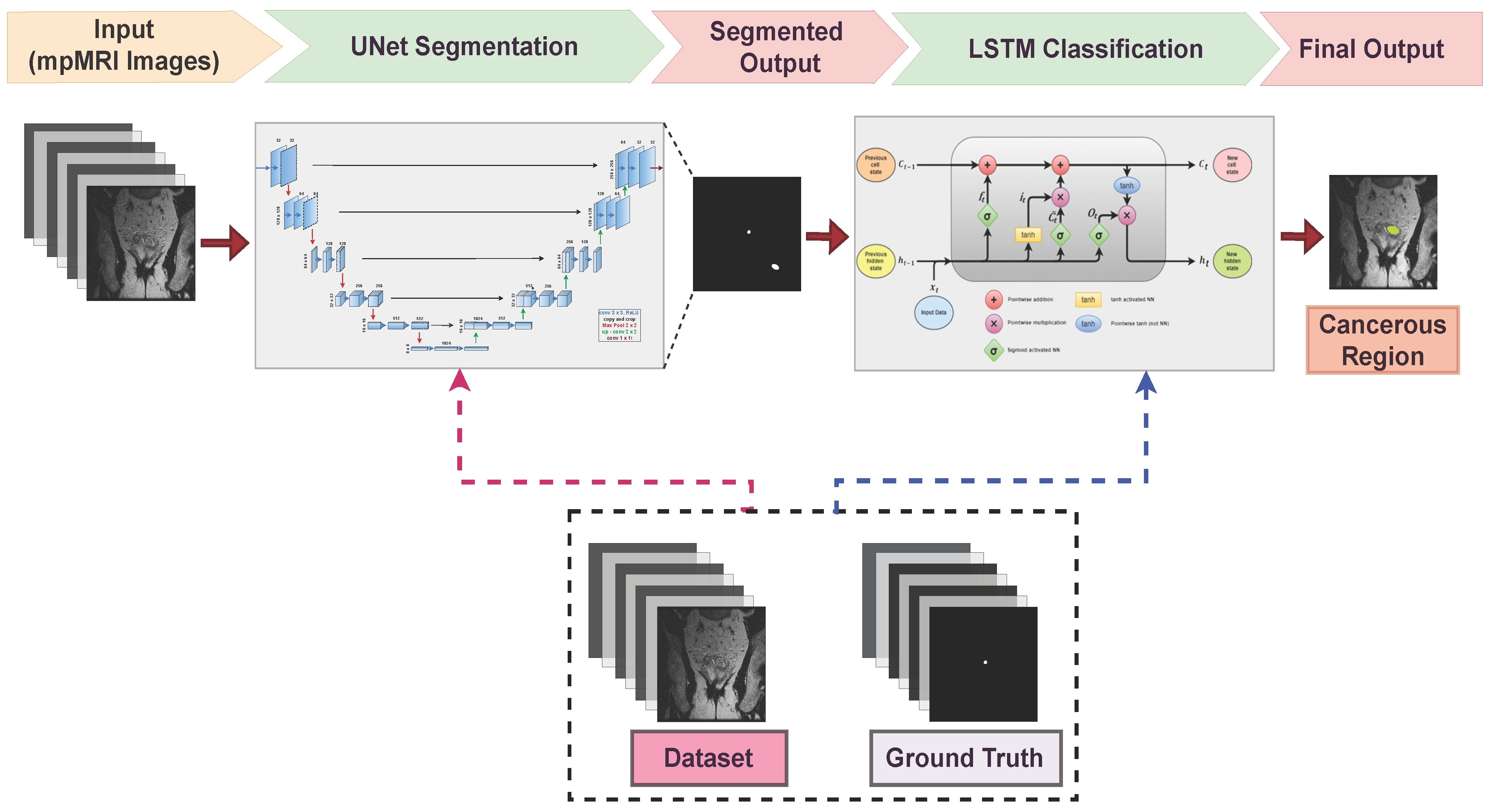
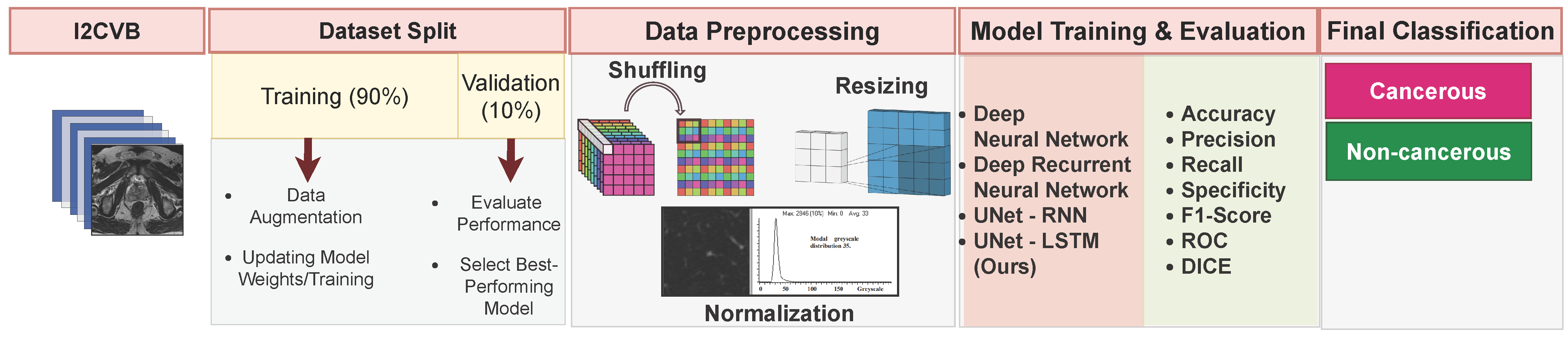
3. Materials and Methods
3.1. Dataset
3.2. Preprocessing
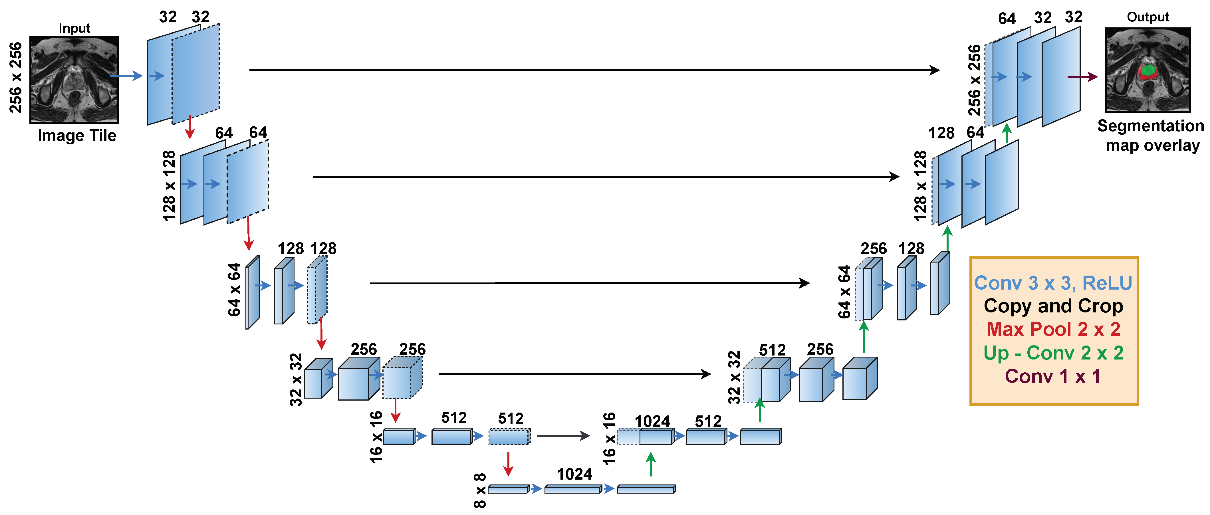
3.3. Segmentation
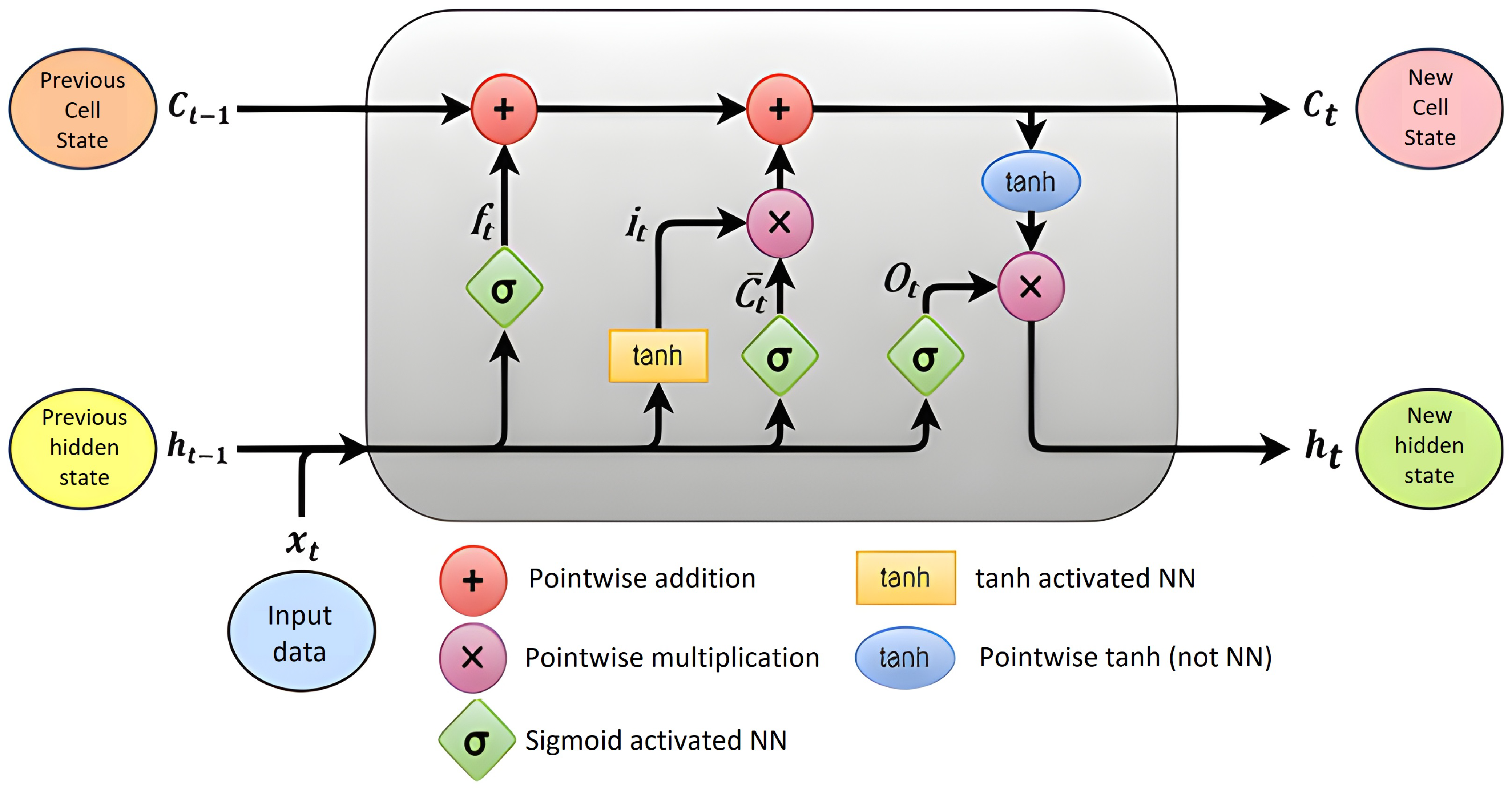
3.4. Classification
3.5. Implementation and Experimental Setup
| Algorithm 1 Training PCa detection from mpMRI. |
|
3.6. Evaluation Metrics
- Precision: Precision is the ratio of TP predictions to the total number of positive predictions. In other words, it measures how many predicted positive cases are positive. A high precision value indicates that the model has a low rate of false positives.
- Recall: Recall, also referred to as sensitivity or true positive rate (TPR), quantifies the ratio of correctly predicted TP cases to the overall number of positive cases. Essentially, it evaluates the accuracy of identifying actual positive cases as positive. In the context of prostate cancer diagnosis, a high recall/sensitivity signifies the algorithm’s capability to accurately detect cancerous tissue.
- F1 score: The harmonic means of precision and recall. In prostate cancer diagnosis, a high F1 score indicates that the algorithm is able to accurately identify cancerous tissue with few false positives and false negatives.
- Accuracy: The accuracy is the proportion of correct predictions made by the algorithm. In prostate cancer diagnosis, high accuracy indicates that the algorithm is able to identify both cancerous and healthy tissue accurately. Accuracy is .
- Specificity: The specificity, also known as the false positive rate (FPR), is the proportion of actual negative cases correctly identified by the algorithm. In prostate cancer diagnosis, high specificity indicates that the algorithm is able to identify healthy tissue accurately.
- Receiver operating characteristic (ROC): The ROC plot illustrates the trade-off between sensitivity and specificity for varying threshold values. To assess the algorithm’s overall performance, the area under the ROC curve, known as AUC, is commonly employed as a metric. The AUC captures the algorithm’s ability to discriminate between positive and negative cases, providing a comprehensive evaluation of its performance.
- Dice similarity coefficient (DSC): The Dice index, also referred to as the Dice coefficient, serves as a commonly used metric for evaluating the performance of a segmentation model. It quantifies the degree of overlap between the predicted segmentation and the ground truth, with values ranging from 0 to 1. A value of 1 signifies a perfect agreement between the predicted and ground truth segmentation. A higher Dice coefficient indicates improved segmentation accuracy, which is particularly valuable when working with imbalanced data or when dealing with segmented objects of varying sizes.
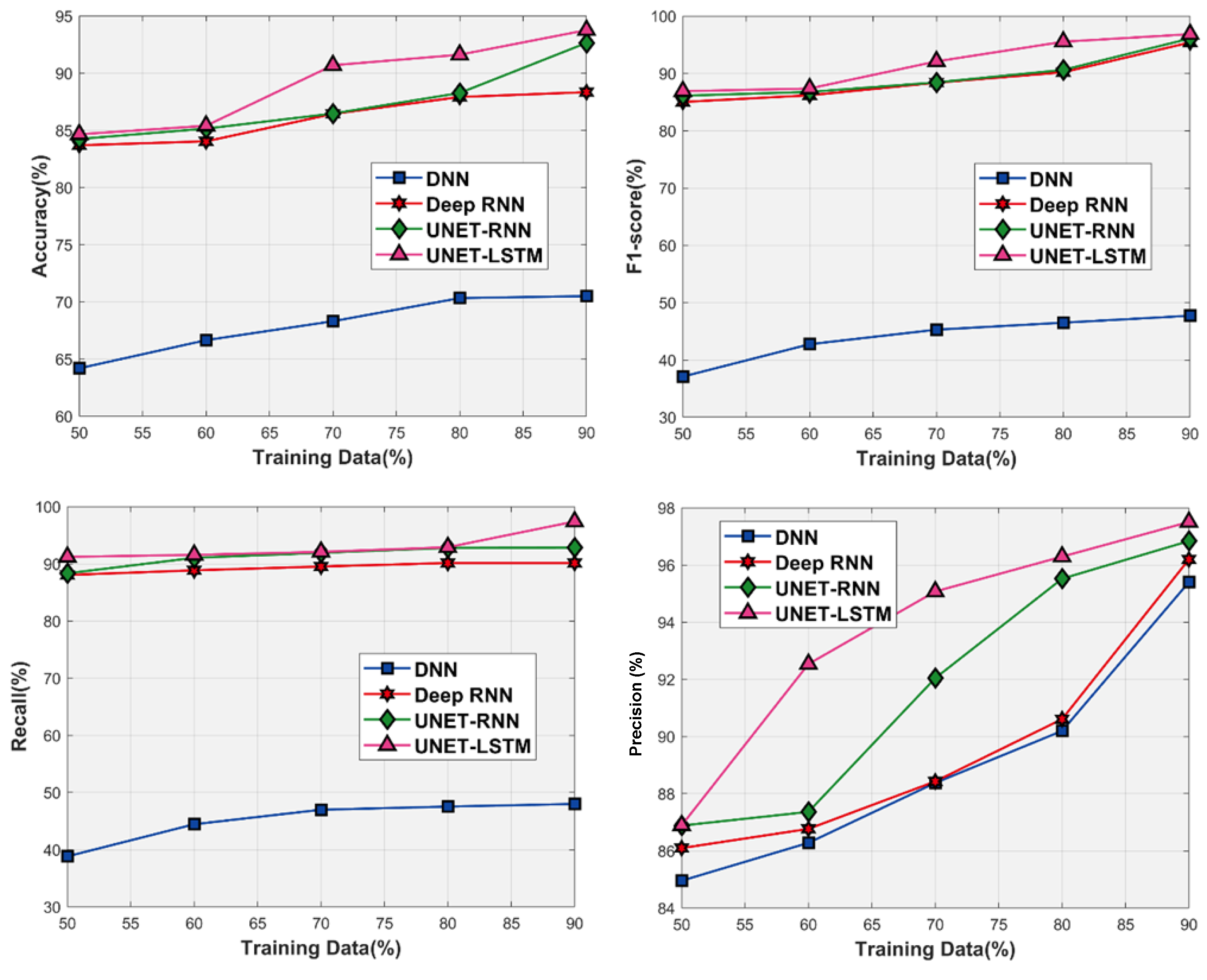
4. Results and Discussion
5. Conclusions
6. Limitations and Future Work
Author Contributions
Funding
Data Availability Statement
Conflicts of Interest
References
- Stephen, W.L.; Larry, E.S.; Hussain, S.; R, I.A.; Taylor, S.S. Prostate Cancer; U.S. National Library of Medicine: Bethesda, MD, USA, 2022.
- Survival Rates for Prostate Cancer; American Cancer Society: Atlanta, GA, USA, 2023.
- Tabatabaei, Z.; Colomer, A.; Engan, K.; Oliver, J.; Naranjo, V. Residual block convolutional auto encoder in content-based medical image retrieval. In Proceedings of the 2022 IEEE 14th Image, Video, and Multidimensional Signal Processing Workshop (IVMSP), Nafplio, Greece, 26–29 June 2022; IEEE: Piscataway, NJ, USA, 2022; pp. 1–5. [Google Scholar]
- Kanwal, N.; Eftestøl, T.; Khoraminia, F.; Zuiverloon, T.C.; Engan, K. Vision Transformers for Small Histological Datasets Learned Through Knowledge Distillation. In Proceedings of the Pacific-Asia Conference on Knowledge Discovery and Data Mining, Osaka, Japan, 25–28 May 2023; Springer: Cham, Switzerland, 2023; pp. 167–179. [Google Scholar]
- Liu, X.; Langer, D.L.; Haider, M.A.; Yang, Y.; Wernick, M.N.; Yetik, I.S. Prostate cancer segmentation with simultaneous estimation of Markov random field parameters and class. IEEE Trans. Med. Imaging 2009, 28, 906–915. [Google Scholar] [CrossRef] [PubMed]
- Kanwal, N.; Amundsen, R.; Hardardottir, H.; Janssen, E.A.; Engan, K. Detection and Localization of Melanoma Skin Cancer in Histopathological Whole Slide Images. arXiv 2023, arXiv:2302.03014. [Google Scholar]
- Kanwal, N.; Pérez-Bueno, F.; Schmidt, A.; Engan, K.; Molina, R. The Devil is in the Details: Whole Slide Image Acquisition and Processing for Artifacts Detection, Color Variation, and Data Augmentation: A Review. IEEE Access 2022, 10, 58821–58844. [Google Scholar] [CrossRef]
- Sunoqrot, M.R.; Selnæs, K.M.; Sandsmark, E.; Langørgen, S.; Bertilsson, H.; Bathen, T.F.; Elschot, M. The reproducibility of deep learning-based segmentation of the prostate gland and zones on T2-weighted MR images. Diagnostics 2021, 11, 1690. [Google Scholar] [CrossRef]
- Cao, R.; Bajgiran, A.M.; Mirak, S.A.; Shakeri, S.; Zhong, X.; Enzmann, D.; Raman, S.; Sung, K. Joint prostate cancer detection and Gleason score prediction in mp-MRI via FocalNet. IEEE Trans. Med. Imaging 2019, 38, 2496–2506. [Google Scholar] [CrossRef] [Green Version]
- Gavade, A.B.; Nerli, R.B.; Ghagane, S.; Gavade, P.A.; Bhagavatula, V.S.P. Cancer Cell Detection and Classification from Digital Whole Slide Image. In Smart Technologies in Data Science and Communication: Proceedings of SMART-DSC 2022; Springer: Singapore, 2023; pp. 289–299. [Google Scholar]
- Tabatabaei, Z.; Engan, K.; Oliver, J.; Naranjo, V. Self-supervised learning of a tailored Convolutional Auto Encoder for histopathological prostate grading. arXiv 2023, arXiv:2303.11837. [Google Scholar]
- Li, H.; Lee, C.H.; Chia, D.; Lin, Z.; Huang, W.; Tan, C.H. Machine learning in prostate MRI for prostate cancer: Current status and future opportunities. Diagnostics 2022, 12, 289. [Google Scholar] [CrossRef]
- Zhang, L.; Li, L.; Tang, M.; Huan, Y.; Zhang, X.; Zhe, X. A new approach to diagnosing prostate cancer through magnetic resonance imaging. Alex. Eng. J. 2021, 60, 897–904. [Google Scholar] [CrossRef]
- Peng, Y.; Jiang, Y.; Yang, C.; Brown, J.B.; Antic, T.; Sethi, I.; Schmid-Tannwald, C.; Giger, M.L.; Eggener, S.E.; Oto, A. Quantitative analysis of multiparametric prostate MR images: Differentiation between prostate cancer and normal tissue and correlation with Gleason score—A computer-aided diagnosis development study. Radiology 2013, 267, 787–796. [Google Scholar] [CrossRef]
- Zhong, X.; Cao, R.; Shakeri, S.; Scalzo, F.; Lee, Y.; Enzmann, D.R.; Wu, H.H.; Raman, S.S.; Sung, K. Deep transfer learning-based prostate cancer classification using 3 Tesla multi-parametric MRI. Abdom. Radiol. 2019, 44, 2030–2039. [Google Scholar] [CrossRef]
- Mehta, P.; Antonelli, M.; Ahmed, H.U.; Emberton, M.; Punwani, S.; Ourselin, S. Computer-aided diagnosis of prostate cancer using multiparametric MRI and clinical features: A patient-level classification framework. Med. Image Anal. 2021, 73, 102153. [Google Scholar] [CrossRef]
- Mehta, P.; Antonelli, M.; Singh, S.; Grondecka, N.; Johnston, E.W.; Ahmed, H.U.; Emberton, M.; Punwani, S.; Ourselin, S. AutoProstate: Towards automated reporting of prostate MRI for prostate cancer assessment using deep learning. Cancers 2021, 13, 6138. [Google Scholar] [CrossRef]
- Brosch, T.; Peters, J.; Groth, A.; Stehle, T.; Weese, J. Deep learning-based boundary detection for model-based segmentation with application to MR prostate segmentation. In Proceedings of the Medical Image Computing and Computer Assisted Intervention–MICCAI 2018: 21st International Conference, Granada, Spain, 16–20 September 2018; Proceedings, Part IV 11. Springer: Cham, Switzerland, 2018; pp. 515–522. [Google Scholar]
- Litjens, G.; Debats, O.; Barentsz, J.; Karssemeijer, N.; Huisman, H. Computer-aided detection of prostate cancer in MRI. IEEE Trans. Med. Imaging 2014, 33, 1083–1092. [Google Scholar] [CrossRef]
- Aldoj, N.; Biavati, F.; Michallek, F.; Stober, S.; Dewey, M. Automatic prostate and prostate zones segmentation of magnetic resonance images using DenseNet-like U-net. Sci. Rep. 2020, 10, 14315. [Google Scholar] [CrossRef]
- Artan, Y.; Haider, M.A.; Langer, D.L.; Van der Kwast, T.H.; Evans, A.J.; Yang, Y.; Wernick, M.N.; Trachtenberg, J.; Yetik, I.S. Prostate cancer localization with multispectral MRI using cost-sensitive support vector machines and conditional random fields. IEEE Trans. Image Process. 2010, 19, 2444–2455. [Google Scholar] [CrossRef]
- Karimi, D.; Samei, G.; Kesch, C.; Nir, G.; Salcudean, S.E. Prostate segmentation in MRI using a convolutional neural network architecture and training strategy based on statistical shape models. Int. J. Comput. Assist. Radiol. Surg. 2018, 13, 1211–1219. [Google Scholar] [CrossRef]
- Tian, Z.; Liu, L.; Zhang, Z.; Fei, B. PSNet: Prostate segmentation on MRI based on a convolutional neural network. J. Med. Imaging 2018, 5, 021208. [Google Scholar] [CrossRef] [PubMed]
- Abraham, B.; Nair, M.S. Automated grading of prostate cancer using convolutional neural network and ordinal class classifier. Inform. Med. Unlocked 2019, 17, 100256. [Google Scholar] [CrossRef]
- Duran, A.; Dussert, G.; Rouvière, O.; Jaouen, T.; Jodoin, P.M.; Lartizien, C. ProstAttention-Net: A deep attention model for prostate cancer segmentation by aggressiveness in MRI scans. Med. Image Anal. 2022, 77, 102347. [Google Scholar] [CrossRef] [PubMed]
- Mahapatra, D.; Buhmann, J.M. Visual saliency-based active learning for prostate magnetic resonance imaging segmentation. J. Med. Imaging 2016, 3, 014003. [Google Scholar] [CrossRef] [Green Version]
- Liu, X.; Samil Yetik, I. Iterative normalization method for improved prostate cancer localization with multispectral magnetic resonance imaging. J. Electron. Imaging 2012, 21, 023008. [Google Scholar] [CrossRef]
- Sun, Z.; Wu, P.; Cui, Y.; Liu, X.; Wang, K.; Gao, G.; Wang, H.; Zhang, X.; Wang, X. Deep-Learning Models for Detection and Localization of Visible Clinically Significant Prostate Cancer on Multi-Parametric MRI. J. Magn. Reson. Imaging 2023. [Google Scholar] [CrossRef]
- Hasan, A.M.; Qasim, A.F.; Jalab, H.A.; Ibrahim, R.W. Breast Cancer MRI Classification Based on Fractional Entropy Image Enhancement and Deep Feature Extraction. Baghdad Sci. J. 2023, 20, 0221. [Google Scholar] [CrossRef]
- Agnes, S.A.; Anitha, J.; Solomon, A.A. Two-stage lung nodule detection framework using enhanced UNet and convolutional LSTM networks in CT images. Comput. Biol. Med. 2022, 149, 106059. [Google Scholar] [CrossRef] [PubMed]
- Lemaître, G.; Martí, R.; Freixenet, J.; Vilanova, J.C.; Walker, P.M.; Meriaudeau, F. Computer-aided detection and diagnosis for prostate cancer based on mono and multi-parametric MRI: A review. Comput. Biol. Med. 2015, 60, 8–31. [Google Scholar] [CrossRef] [PubMed] [Green Version]
- Ronneberger, O.; Fischer, P.; Brox, T. U-net: Convolutional networks for biomedical image segmentation. In Proceedings of the Medical Image Computing and Computer-Assisted Intervention–MICCAI 2015: 18th International Conference, Munich, Germany, 5–9 October 2015; Proceedings, Part III 18. Springer: Cham, Switzerland, 2015; pp. 234–241. [Google Scholar]
- Staudemeyer, R.C.; Morris, E.R. Understanding LSTM—A tutorial into long short-term memory recurrent neural networks. arXiv 2019, arXiv:1909.09586. [Google Scholar]
- Armato, S., III; Huisman, H.; Drukker, K.; Hadjiiski, L.; Kirby, J.; Petrick, N.; Redmond, G.; Giger, M.; Cha, K.; Mamonov, A.; et al. PROSTATEx Challenges for computerized classification of prostate lesions from multiparametric magnetic resonance images. J. Med. Imaging 2018, 5, 044501. [Google Scholar] [CrossRef] [PubMed]
- Simmons, L.A.; Kanthabalan, A.; Arya, M.; Briggs, T.; Barratt, D.; Charman, S.C.; Freeman, A.; Gelister, J.; Hawkes, D.; Hu, Y.; et al. The PICTURE study: Diagnostic accuracy of multiparametric MRI in men requiring a repeat prostate biopsy. Br. J. Cancer 2017, 116, 1159–1165. [Google Scholar] [CrossRef] [PubMed]
- Kanwal, N.; Rizzo, G. Attention-based clinical note summarization. In Proceedings of the 37th ACM/SIGAPP Symposium on Applied Computing, Virtual, 25–29 April 2022; pp. 813–820. [Google Scholar]


| Architectures | Accuracy (%) | F1 (%) | Precision | Recall (Sens. (%)) | RoC | Spec. (%) | Dice |
|---|---|---|---|---|---|---|---|
| Liu et al. [5] | 89.38 | - | - | 87.5 | - | 89.5 | 0.62 |
| Artan et al. [21] | - | - | - | 85.0 | - | 50.0 | 0.34 |
| Zhang et al. [13] | 80.97 | - | 76.69 | - | 0.77 | - | - |
| PCF-SEL-MR [16] | - | - | 63.0 | 75.0 | 0.86 | 55.0 | - |
| FocalNet [9] | - | - | - | 89.7 | - | - | - |
| DNN | 68.31 | 45.28 | 88.38 | 46.98 | 0.719 | 89.53 | 0.59 |
| Deep RNN | 86.43 | 88.37 | 88.43 | 89.53 | 0.787 | 91.81 | 0.64 |
| U-Net RNN | 86.47 | 88.43 | 92.04 | 91.92 | 0.814 | 90.09 | 0.65 |
| U-Net LSTM (Ours) | 90.69 | 92.09 | 95.17 | 92.09 | 0.953 | 96.88 | 0.67 |
Disclaimer/Publisher’s Note: The statements, opinions and data contained in all publications are solely those of the individual author(s) and contributor(s) and not of MDPI and/or the editor(s). MDPI and/or the editor(s) disclaim responsibility for any injury to people or property resulting from any ideas, methods, instructions or products referred to in the content. |
© 2023 by the authors. Licensee MDPI, Basel, Switzerland. This article is an open access article distributed under the terms and conditions of the Creative Commons Attribution (CC BY) license (https://creativecommons.org/licenses/by/4.0/).
Share and Cite
Gavade, A.B.; Nerli, R.; Kanwal, N.; Gavade, P.A.; Pol, S.S.; Rizvi, S.T.H. Automated Diagnosis of Prostate Cancer Using mpMRI Images: A Deep Learning Approach for Clinical Decision Support. Computers 2023, 12, 152. https://doi.org/10.3390/computers12080152
Gavade AB, Nerli R, Kanwal N, Gavade PA, Pol SS, Rizvi STH. Automated Diagnosis of Prostate Cancer Using mpMRI Images: A Deep Learning Approach for Clinical Decision Support. Computers. 2023; 12(8):152. https://doi.org/10.3390/computers12080152
Chicago/Turabian StyleGavade, Anil B., Rajendra Nerli, Neel Kanwal, Priyanka A. Gavade, Shridhar Sunilkumar Pol, and Syed Tahir Hussain Rizvi. 2023. "Automated Diagnosis of Prostate Cancer Using mpMRI Images: A Deep Learning Approach for Clinical Decision Support" Computers 12, no. 8: 152. https://doi.org/10.3390/computers12080152