
Spatiotemporal Dynamics of a Diffusive Immunosuppressive Infection Model with Nonlocal Competition and Crowley–Martin Functional Response

Department of Mathematics, Northeast Forestry University, Harbin 150040, China
*
Author to whom correspondence should be addressed.
Axioms 2023, 12(12), 1085; https://doi.org/10.3390/axioms12121085
Submission received: 23 October 2023
/
Revised: 23 November 2023
/
Accepted: 24 November 2023
/
Published: 27 November 2023
(This article belongs to the Special Issue Recent Advances in Applied Mathematics and Artificial Intelligence)
Abstract
:In this paper, we introduce the Crowley–Martin functional response and nonlocal competition into a reaction–diffusion immunosuppressive infection model. First, we analyze the existence and stability of the positive constant steady states of the systems with nonlocal competition and local competition, respectively. Second, we deduce the conditions for the occurrence of Turing, Hopf, and Turing–Hopf bifurcations of the system with nonlocal competition, as well as the conditions for the occurrence of Hopf bifurcations of the system with local competition. Furthermore, we employ the multiple time scales method to derive the normal forms of the Hopf bifurcations reduced on the center manifold for both systems. Finally, we conduct numerical simulations for both systems under the same parameter settings, compare the impact of nonlocal competition, and find that the nonlocal term can induce spatially inhomogeneous stable periodic solutions. We also provide corresponding biological explanations for the simulation results.
Keywords:
immunosuppressive infection model; Crowley–Martin functional response; nonlocal competition; Hopf bifurcation; delayMSC:
37G05; 37N25; 35R101. Introduction
Continued infection with certain human pathogens can lead to the development of chronic diseases, such as Hepatitis B Virus (HBV), Hepatitis C Virus (HCV), and Human Immunodeficiency Virus (HIV) [1]. Although specific antiviral treatments are essential for managing these infections, the complete eradication of these pathogens remains an elusive goal due to the high genetic variability of these viruses and their ability to evade the host immune system. In recent years, a few HIV-infected individuals, known as elite controllers, have been discovered [2,3]. They can maintain low or undetectable viral loads without treatment, possibly due to their robust immune responses [4,5,6]. Enhancing virus-specific immune responses is now a key research focus.
Mathematical models have been used to model the dynamic behavior of immune suppression infections between viruses and the immune system [7,8,9]. Komarova et al. [1] proposed a basic immunosuppressive infection model in which the proliferation term of immune cells is considered to be influenced by both viruses and immune cells, expressed as , where c is the immune intensity, stands for the inhibitory effects of the virus on the proliferation of immune cells, and u and v represent the density of viruses and immune cells at time t, respectively.
Following this, many scholars continuously modified the immunosuppressive infection model [10,11,12]. Due to the immune system requiring a time lag to generate new immune cells through a series of events [13], Shu et al. [10] proposed an assumption that the activation rate of immune cells at time t is dependent on both the virus load and the number of immune cells at time . They investigated the immune expansion function described as . In this way, the time delay can be seen as the period during which the immune cells undergo activation or maturation. In other words, these immune cells are produced at time but do not work until t. Subsequently, Li et al. [12] made further modification to the immune expansion function; they proposed that the expansion of immune response is achieved through the stimulation of the virus on the immune cells. This process involves the processing and presentation of viral antigens by antigen-presenting cells for recognition and activation of effector cells [14]. This implies that it takes a certain amount of time for the virus to effectively stimulate the immune cells, which is known as the viral stimulation delay, denoted by . In this way, the immune cells at time t are activated by the virus that stimulated them at time . They investigated the immune expansion function described as . The latest advancements in this model involve the work of Chen et al. [15], where they replaced the immune expansion function with the Beddington–DeAngelis (B-D) functional response given by:
where s represents the competition intensity among immune responses. Additionally, Xue et al. [16] introduced diffusion into the model proposed by Chen et al. [15].
In this paper, we consider replacing the Beddington–DeAngelis functional response with the Crowley–Martin (C-M) functional response:
The Crowley–Martin functional response was first introduced by Crowley and Martin [17]. Like the B-D functional response, it was initially used to describe interactions and competitive relationships in predator–prey models [18,19,20]. Skalski et al. [21] analyzed an important distinction between the B-D functional response and the C-M functional response in predator–prey models through mathematical formulas; they suggested using the B-D functional response when the predator’s consumption rate is no longer correlated with predator density at high prey densities, whereas they advised employing the C-M functional response when the predator’s consumption rate continues to be influenced by higher predator densities at high prey densities.
Now, revisiting the immunosuppressive infection model, when the viral quantity is sufficiently high, the B-D functional response can be expressed mathematically as:
while the C-M functional response can be expressed as:
From this, it can be observed that as the density of viruses (denoted as u) increases, in the B-D functional response, the competition among immune cells (represented by s) has almost no effect on their proliferation rate. However, in the C-M functional response, competition among immune cells still affects their proliferation rate. In reality, as viral quantity rises, it can harm the immune system, leading to immune exhaustion. This exhaustion makes it challenging for immune cells to efficiently clear the virus, resulting in a weakened immune response (as mentioned in [22]). Even when only a small fraction of immune cells are actively responding to the viruses, some level of competition among them can influence their proliferation rate, functionality, and lifespan, thus affecting the overall immune response (as mentioned in [23]). This implies that even though the viral quantity reaches a certain threshold, competition s among immune cells still influences the proliferation term of immune cells, aligning more closely with the description of the C-M functional response. Therefore, it is reasonable to replace the B-D functional response with the C-M functional response. In fact, many scholars have incorporated the C-M functional response into virus infection models [24,25,26,27], primarily to simulate the infection rate. To the best of our knowledge, there have been relatively few instances of utilizing the C-M functional response to simulate the proliferation term of immune cells in these models.
In this paper, we will consider the following system:
where . The variables and represent the density of viruses and immune cells at the spatial location x and time t, respectively. The parameters a and b correspond to the natural mortality rates of the viruses and immune cells, respectively. Meanwhile, r and K describe the viral replication rate and viral load, respectively. Additionally, we use the parameters c, s, and to represent the immune intensity, the competition intensity among immune responses, and the inhibitory effects of the viruses on the proliferation of immune cells. The parameter characterizes the viral stimulation delay, which means the immune cells at time t are activated by the virus that stimulated them at time . It is postulated that immune cells eliminate viruses at a rate of , while viruses suppress immune cells at a rate of . The diffusion rates for the viruses and immune cells are denoted as and , respectively. It is crucial to emphasize that all parameters in system (1) must remain nonnegative.
Nonlocal competition was first proposed by Furter and Grinfeld in their research in 1989 [28]. They introduced nonlocal interactions into a population dynamics model of a single species to describe how species interact when competing for a shared resource. In recent years, many reaction–diffusion equations with nonlocal competition have been used in ecological system modeling [29,30,31,32]. Research indicates that introducing nonlocal effects may lead to the emergence of multi-peaked population density distributions [32,33,34]. In system (1), the viral replication rate follows logistic growth, . That implies that there is an implicit one-to-one correspondence between viral and infected cell, while Bessonov et al. [35] and Banerjee et al. [36] mentioned that, in biomedical applications, viral cells can also compete for resources, with the possibility of different types of viral cells infecting the same cell. In this case, the viral reproduction rate is described by the expression , where is some reasonable kernel which characterizes the efficacy of host cell infection. The integral corresponds to nonlocal resource consumption at a particular spatial point x [31]. In this paper, we choose . In order to investigate the influence of nonlocal competition on the dynamic behavior of system (1), we also consider the following system with nonlocal competition:
where all the parameters are consistent with those in system (1).
The remaining sections of the paper are structured as follows. In Section 2, we separately discuss the stability of positive constant steady states and the existence of possible bifurcations for systems with and without nonlocal competition. Section 3 presents the normal forms of Hopf bifurcations in both systems and analyzes the stability of bifurcating periodic solutions, along with their respective bifurcation directions. In Section 4, we conduct numerical simulations for the two systems to compare the distinct spatiotemporal dynamics arising from the introduction of nonlocal competition. Finally, conclusions are given in Section 5.
2. Stability and Bifurcation
2.1. Stability and Bifurcation of the System with Nonlocal Competition
Considering the biological aspect, we focus on the positive constant steady state of system (2). Then we have:
Suppose
Then by direct calculation, we can deduce the form of as follows:
Denote
For the sake of discussing the existence of positive constant steady states, we make the following assumptions:
Theorem 1.
Assume that (H0) holds; then for the positive constant steady state of system (2), the following statements hold true.
Proof.
Note that and is a quadratic equation. Then we will analyze the monotonicity of based on the direction of and the presence of the positive roots of to determine the number of positive roots of .
If , then the parabola of opens downward and has two positive roots and . That means is monotonically increasing when , and monotonically decreasing when . At this time, we have the following results.
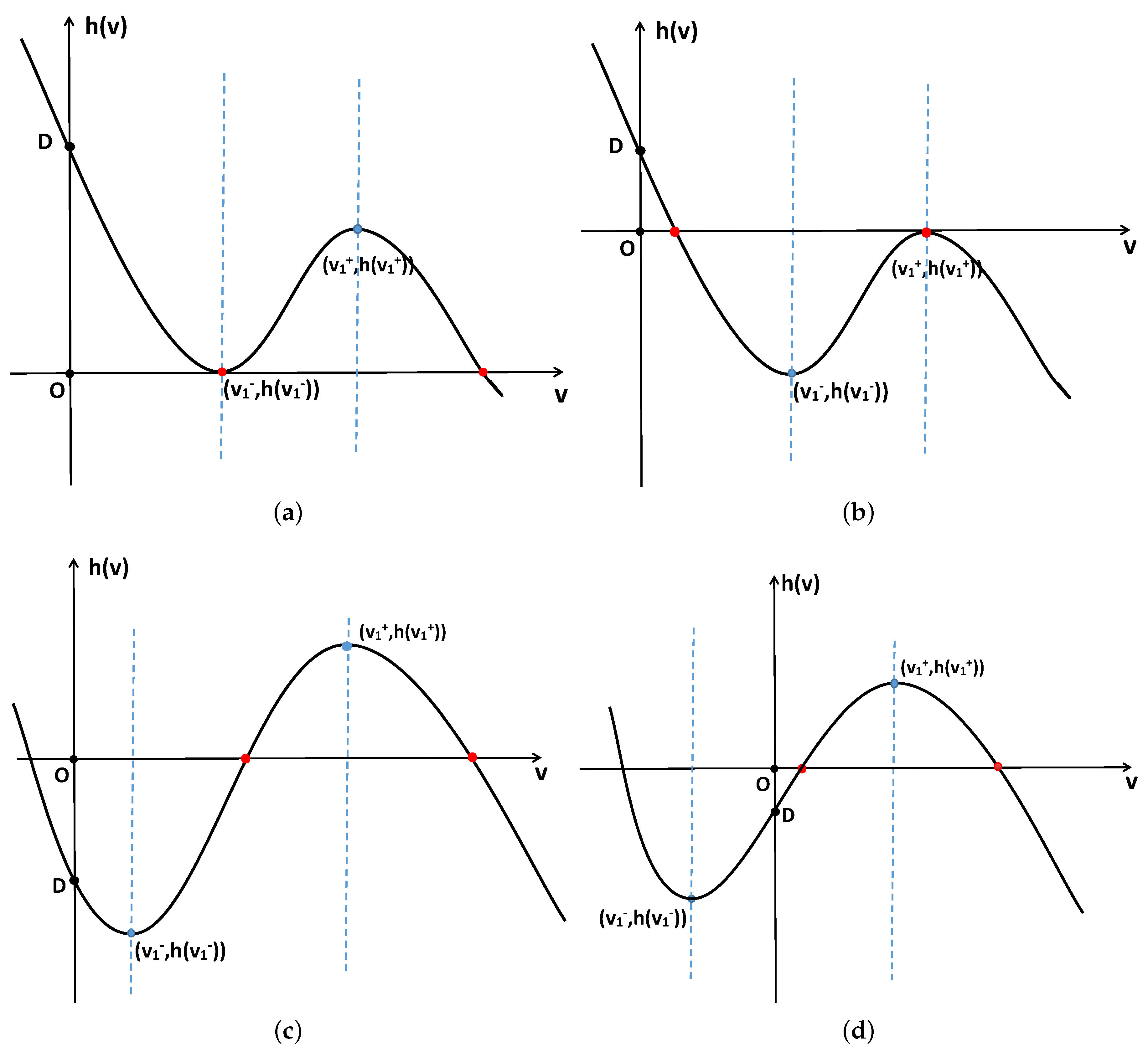
If , no matter the sign of B, the parabola of always opens downward, and has one positive root and one negative root . That means is monotonically increasing when , and monotonically decreasing when . Combining this with , we can conclude that has two positive roots (see Figure 2d).
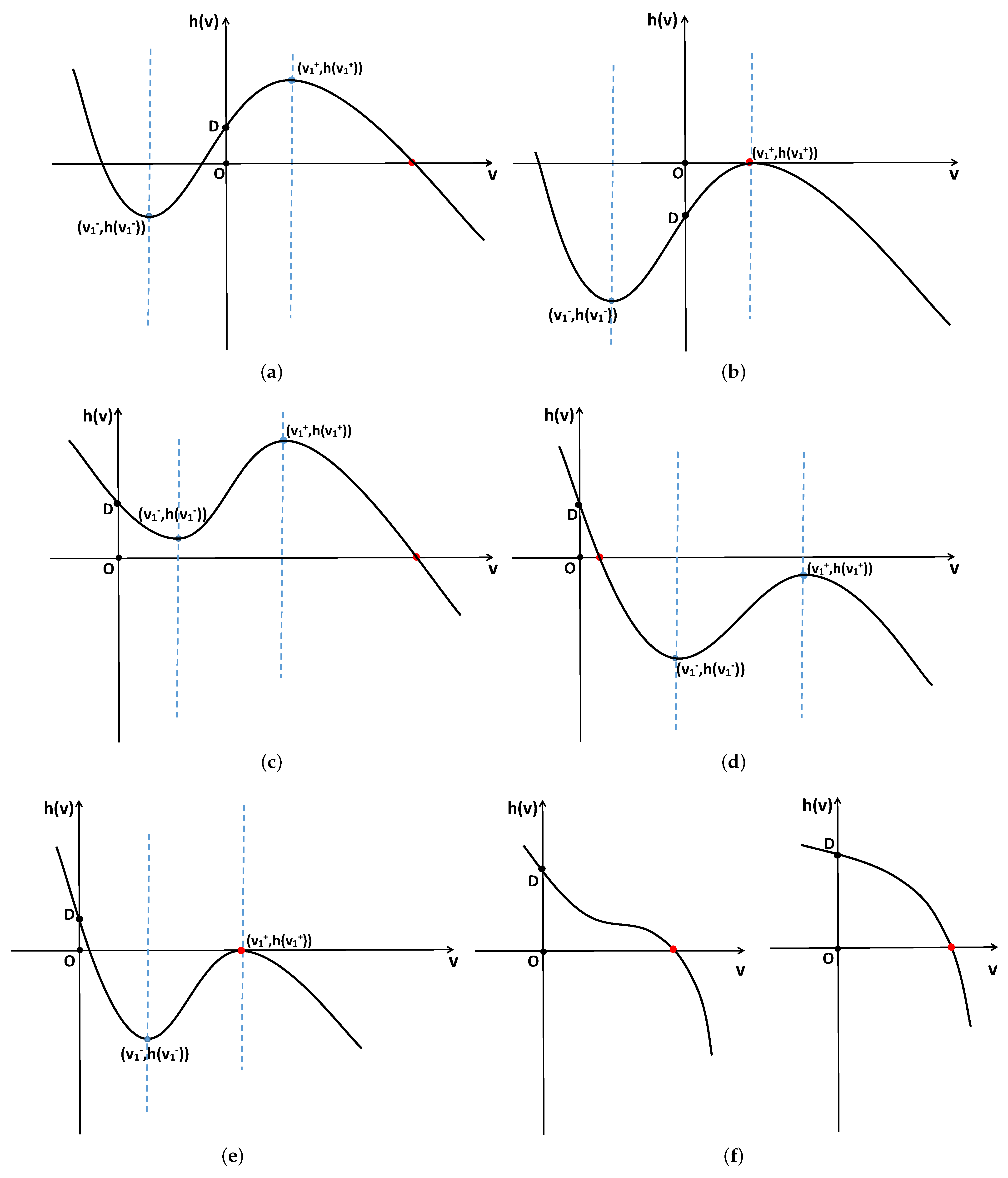
This proves (i) and (ii). Similarly, we conclude (iii), the remaining proof process is omitted, and we only provide graphs for one positive root (see Figure 3). □
Denote the positive constant steady states of system (2) as . Therefore, when the parameters of system (2) satisfy any one of conditions (i)–(iii) of Theorem 1, the positive constant steady state exists.
Clearly, , and are all positive numbers.
Therefore, the associated characteristic equations at are
with
and
Case 1
When , Equation (9) becomes
Suppose that there exists such that for ; then the characteristic Equation (10) has a zero root for . Futhermore, note that is monotonically increasing with respect to n, so if and only if . Take K as a bifurcation parameter, and assume that the transversality condition for the occurrence of 0-mode Turing bifurcation is satisfied. Then we have the following results.
Theorem 2.
If holds, and , then we have the following statements.
- (i)
- (ii)
- (iii)
Case 2
Set as a root of Equation (9); then we have
Futhermore, we define
By squaring both equations in Equation (11) and adding them together, then denoting , we can obtain
Lemma 1.
Proof.
By simple calculation, we can obtain
and
Then we conclude that, for , there always exist and . Futhermore, if holds, we can obtain .
The results mentioned above suggest that there is a unique positive root satisfying Equation (13), then Equation (9) has a unique pair of purely imaginary roots , where . Furthermore, due to , we have . From Equation (12), we can derive the form of as shown in Equation (14). This completes the proof. □
Remark 1.
We can deduce from Equation (14) that for a fixed value of , attains its minimum at . Define this smallest critical value as:
Lemma 2.
For system (2), the transversality condition for the occurrence of -mode Hopf bifurcation is satisfied, that is, , for
Proof.
Differentiating both sides of Equation (9) with respect to the time delay results in
From Equation (9) we can obtain that, for all , there always exists . Then substituting it into the above formula, we can obtain
This completes the proof. □
Theorem 3.
Assuming that and are satisfied, for system (2), we have the following statements.
- (i)
- When and , the positive constant steady state is locally asymptotically stable for and unstable for . Additionally, system (2) undergoes -mode Hopf bifurcation at when ;
- (ii)
- When , the positive constant steady state is unstable for ;
- (iii)
- When , then system (2) undergoes -mode Turing–Hopf bifurcation at ,
where is defined in Equation (15), and satisfies .
2.2. Stability and Bifurcation of the System without Nonlocal Competition
In fact, the positive constant steady states of system (2) with nonlocal competition are identical to those of system (1) without nonlocal competition; they all align with the description provided in Theorem 1. Then, the characteristic equation of the linearization of system (1) at is
where
where are defined as in Equation (8).
By the same approach as in Section 2.1, we have the following results:
Theorem 4.
The specific proof process is omitted.
3. Stability and Direction of Hopf Bifurcation
In this section, we will use the method of multiple time scales to analyze the stability and direction of Hopf bifurcation for the two systems.
Denote
and
Expand by using a Taylor series around , leading to
3.1. Stability and Direction of Hopf Bifurcation of the System with Nonlocal Competition
We have obtained that when , the characteristic equation (9) of the linearization of system (2) has a unique pair of purely imaginary roots , where is defined in (15). At this time, system (2) undergoes -mode Hopf bifurcation at .
Choose the delay as a bifurcation parameter, by setting and translating the equilibrium points of system (2) to the origin; we can express the truncation up to the third-order form of system (2) as follows:
where and are defined as Equation (18).
Denote the eigenvector of the characteristic matrix of system (20) at corresponding to the eigenvalue as , and the eigenvector of the adjoint matrix corresponding to the eigenvalue as ; they satisfy the inner product
Then we have
Set , where represents the critical point for the Hopf bifurcation, as defined in Equation (15). Here, serves as a small perturbation parameter, and is the characteristic scale used for non-dimensionalization. Next, we only present the main results regarding the computation of the normal form for Hopf bifurcation. The specific computational process is detailed in Appendix A.
By the method of multiple time scales, we deduce the normal form of the -mode Hopf bifurcation for system (2) reduced on the center manifold as follows:
where M and are given in Equation (A11) and Equation (A17) in Appendix A.
Now introduce and substitute it into the normal form Equation (22). This yields:
Regarding the stability of the bifurcating periodic solutions of system (2), the following result can be established:
Theorem 5.
When , system (2) has periodic solutions near the positive constant steady state . Moreover:
- (i)
- If , the bifurcating periodic solutions reduced on the center manifold are unstable, and when ( ), the direction of bifurcation is forward (backward);
- (ii)
- If , the bifurcating periodic solutions reduced on the center manifold are stable, and when ( ), the direction of bifurcation is forward (backward).
3.2. Stability and Bifurcation of the System without Nonlocal Competition
Similar to the analysis in reference [16], we can also obtain the normal form of the -mode Hopf bifurcation for system (1) reduced on the center manifold:
where
with
and
The remaining parameters can be found in Appendix A and Equation (17).
4. Numerical Simulations
In this section, we will conduct numerical simulations to demonstrate the theoretical findings we have obtained in the preceding sections. For both system (2) and system (1), we select the same set of parameters as follows:
4.1. Numerical Simulations of the System with Nonlocal Competition
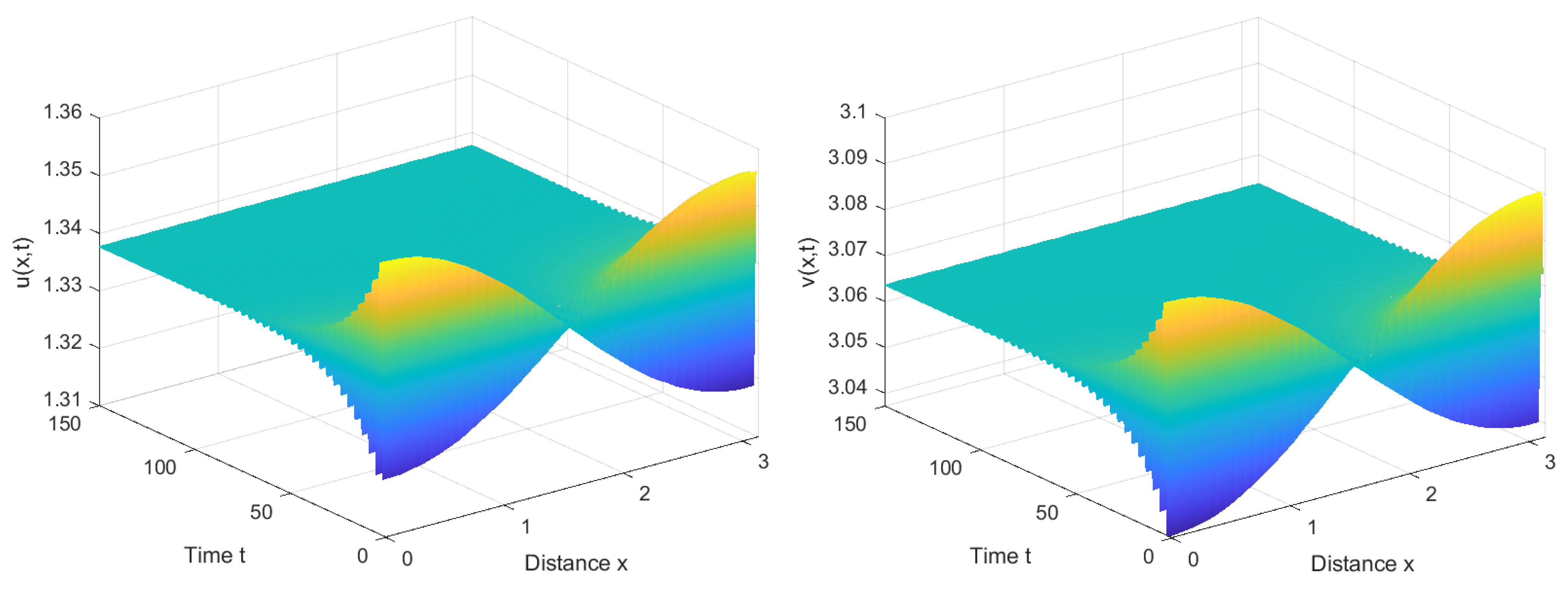
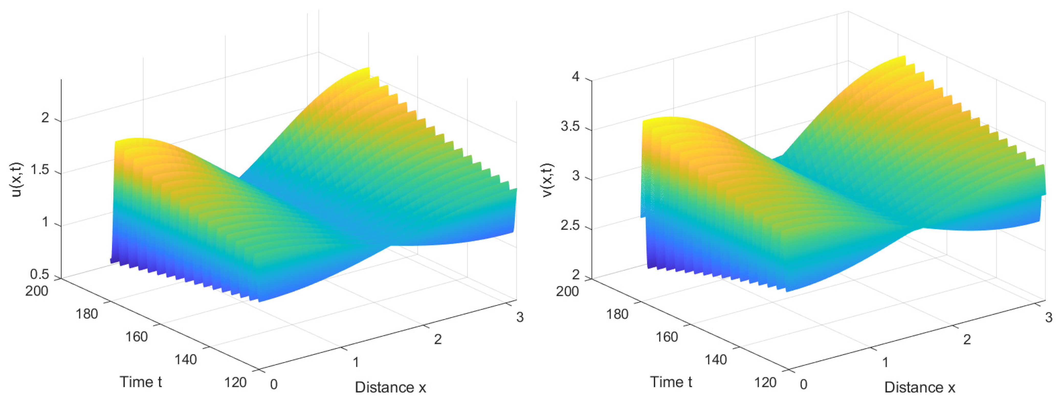
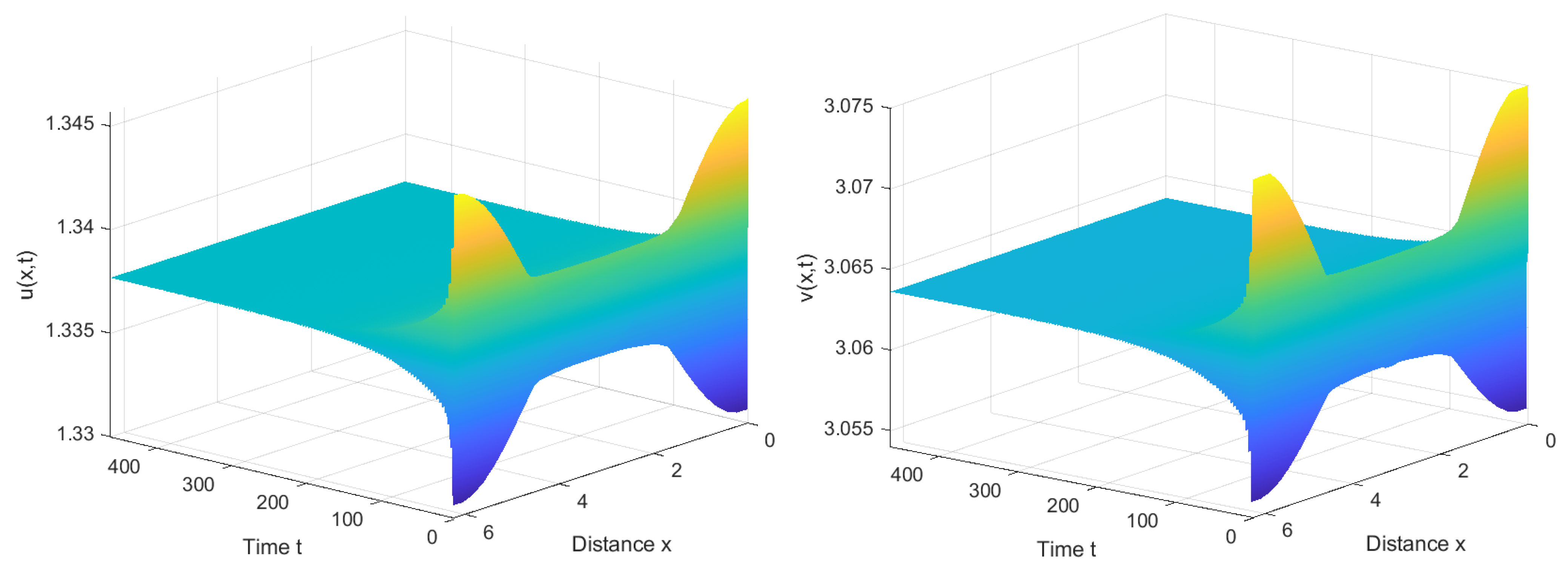
According to Lemma 1 and (15), we can obtain that , , . And the critical point for the Hopf bifurcation is . Furthermore, according to (A11) and (A17), we can calculate that . Hence, when , we can deduce from Theorem 3 that is locally asymptotically stable, as shown in Figure 4; when , we can infer from Theorems 3 and 5 that is unstable and system (2) has stable forward bifurcating periodic solutions near , as shown in Figure 5. When significantly exceeds the critical value , system (2) no longer exhibits stable periodic solutions and will undergo substantial oscillations, as shown in Figure 6.
Remark 2.
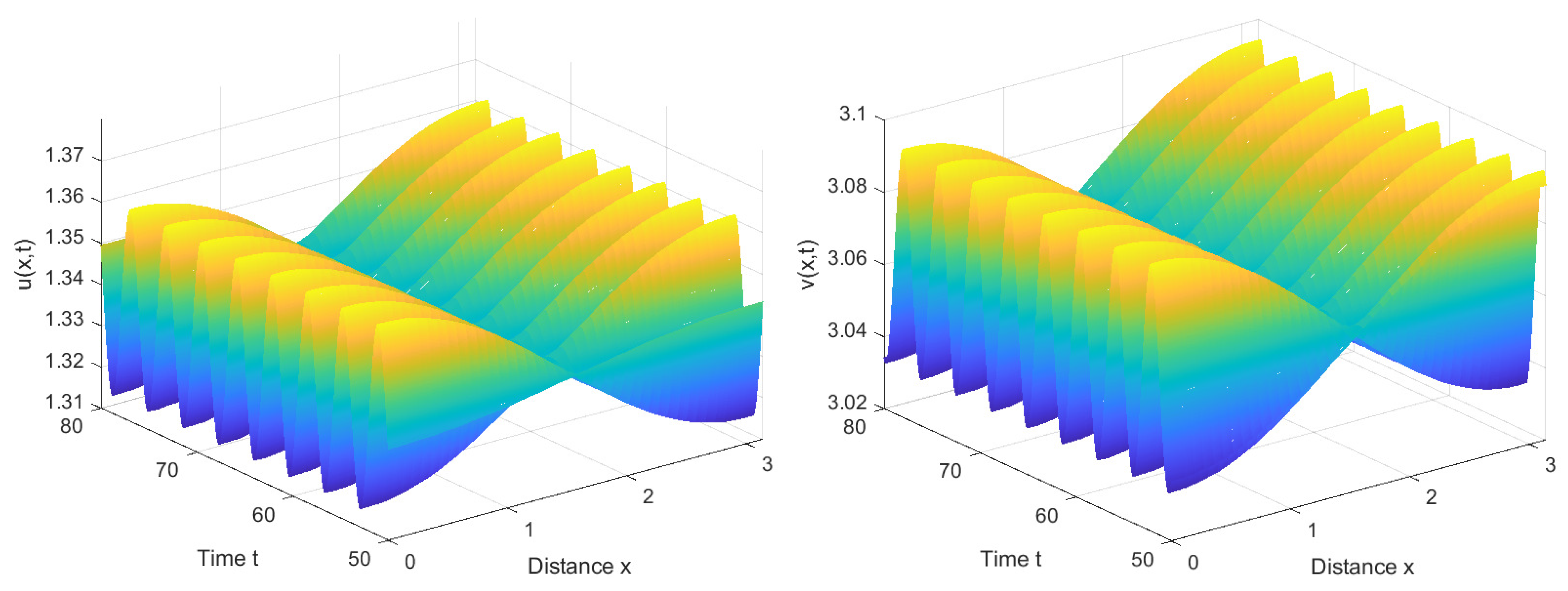
From Figure 4, it can be observed that when the time delay τ required for immune cells to generate an immune response is less than the critical value , system (2) undergoes a period of oscillations before eventually converging to a stable state. This implies that when the immune system is stimulated by the virus, it takes some time to mount an immune response, but eventually manages to control the number of viruses within a certain range. In this scenario, the disease is brought under control, and the quantities of viruses and immune cells no longer exhibit significant fluctuations.
Remark 3.
From Figure 5, it can be observed that when the delay τ required for immune cells to generate an immune response is slightly greater than the critical value , system (2) loses its original stable state and generates spatially inhomogeneous periodic solutions. This occurrence encapsulates the intricate dynamics between viruses and the immune system. When viruses trigger an immune response, immune cells swiftly localize and eliminate local viruses, leading to a decline in the local virus population. However, the nonlocal effect implies that the immune system has a certain sensing range and can perceive the density of viruses in distant areas. This results in the immune system generating a stronger immune response when it senses areas with a high density of viruses in other locations, to combat viruses at a distance. Consequently, the dynamism in viruses and immune cells across the system becomes non-uniform, exhibiting periodic spatial fluctuations. This results in varying dominance; in some regions, the immune system prevails, effectively clearing viruses, while in others, viruses regain dominance. These spatially driven periodic oscillations stem from the intricate interplay between the immune system and viruses, underscoring the complex dynamics of their interaction. The detailed mathematical analysis emphasizes the crucial role played by nonlocal competition in the emergence of spatial inhomogeneity, highlighting its impact on the system’s dynamics.
We have also observed a stable number of cells in the central space, while the cell count on both sides exhibits periodic fluctuations. This phenomenon may be related to the boundary conditions. When immune cells localize to areas with higher virus density, they congregate at the boundary due to the inability to traverse it. As the virus density decreases at the boundary, the nonlocal competition suggests that the immune cells might hypothetically move in the opposite direction, resulting in periodic variations in the number of immune cells on both sides of the boundary. With nearly equivalent counts of immune cells in both forward and backward diffusion trends, the number of immune cells in the central space tends to stabilize.
4.2. Numerical Simulations of the System without Nonlocal Competition
Based on the parameters in (26), the positive constant steady states in system (1) equal the positive constant steady state in system (2), indicating that
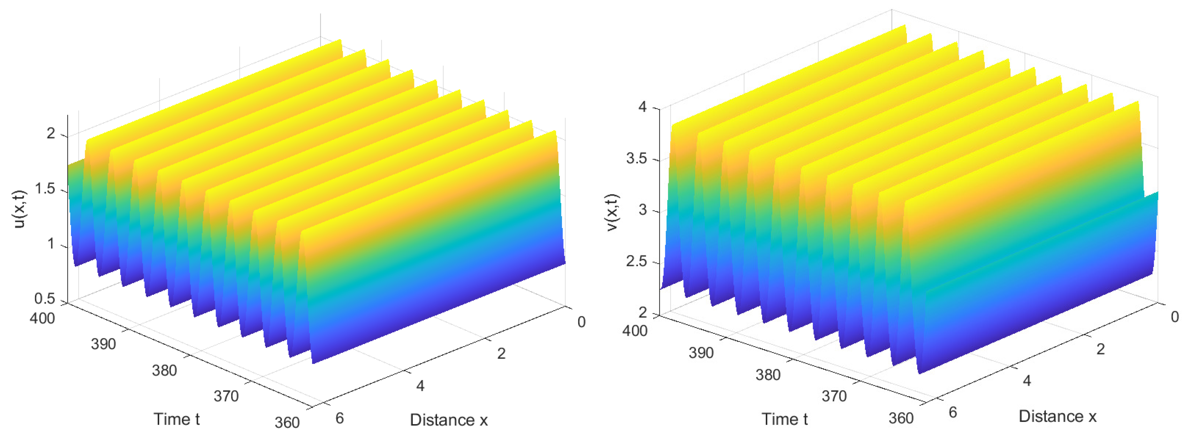
Similarly, by calculation, we find . Therefore, is locally asymptotically stable when , as shown in Figure 7, and unstable when . Furthermore, system (1) also has stable bifurcating periodic solutions and the direction of the Hopf bifurcation is also forward, as shown in Figure 8.
Remark 5.
Under the identical parameter settings, a noticeable difference is observed between the reaction–diffusion system (1) without nonlocal competition and system (2) incorporating nonlocal competition terms. Specifically, in the former case, the critical value is comparatively larger, whereas, in contrast, system (2), with nonlocal competition, exhibits a smaller critical value. Furthermore, Figure 8 demonstrates that system (1) also exhibits periodic and steady state solutions. However, a pivotal disparity emerges regarding the nature of these solutions.
In the context of system (1), the solutions appear spatially homogeneous, indicating an independence of the interaction between the immune system and viruses from spatial variables. This suggests that in the absence of nonlocal competition, the dynamics of the immune response to viruses remain consistent throughout space.
However, a more realistic scenario warrants consideration, suggesting that the interaction between the immune system and viruses should be influenced by spatial variables. In systems where nonlocal competition terms are present, the smaller critical value implies that spatial influences significantly impact the dynamics of the immune system–virus interaction. This signifies a spatial dependency, wherein the behavior of the immune system in response to viruses may vary across different spatial regions, emphasizing the importance of spatial considerations in understanding the dynamics of virus–immune system interactions.
5. Conclusions
This paper introduced the Crowley–Martin functional response into an immunosuppressive infection model and conducted a comparative analysis of the dynamic behavior between a delayed reaction–diffusion system with nonlocal viral competition and a delayed reaction–diffusion system without nonlocal viral competition. The nonlocal term represents the space-time weighted average of the viral population. We derived the normal forms of the Hopf bifurcations reduced on the center manifold for both systems, one with nonlocal competition and the other without, and performed numerical simulations. The results indicated that the introduction of nonlocal competition causes a reduction in the stability region, i.e., , and the system with nonlocal competition generated spatially inhomogeneous periodic solutions, whereas the reaction–diffusion system without nonlocal competition terms yielded spatially homogeneous solutions. This suggested that systems with nonlocal effects exhibited more diverse dynamic behaviors, highlighting the special biological significance of spatiotemporal nonlocality.
Author Contributions
Writing—original draft preparation, Y.X.; funding acquisition, J.X.; methodology, J.X.; supervision, Y.D. All authors have read and agreed to the published version of the manuscript.
Funding
This study was funded by Fundamental Research Funds for the Central Universities of China (Grant No. 2572022DJ07).
Data Availability Statement
No new data were created in this study. Data sharing is not applicable to this article.
Conflicts of Interest
The authors declare no conflict of interest.
Appendix A
The time derivative is now transformed into
with
Set
where . Then we have
To handle the delayed terms, we can approximate as ; thus, we obtain:
with .
Substituting Equations (A1)–(A6) into system (20) results in a set of perturbation equations. Extract the coefficients of the terms:
where are given by Equation (18). Hence, the solution to Equation (A7) can be represented in the following form:
where are defined by Equation (21), and denotes the complex conjugate of the preceding term. Next, collecting the coefficient of , we can obtain
where and are determined by Equation (18). After substituting solution (A8) into the right side of Equation (A9) and simplifying, we define the coefficient vector of as . It is important to note that must satisfy the solvability condition:
Then one has
where
with
Assume that the solution of Equation (A9) takes the form
To facilitate the determination of the coefficients for the second-order solution (A12), we denote
After substituting Equations (A8) and (A12) into Equation (A9) and simplifying, we take the inner product with on both sides of the resulting equation, where . By summing up the obtained results, we can then compare the coefficients in front of the terms and , leading to
where
By calculating, we discover that for , if and only if . Therefore, we can deduce the specific form of solution (A12):
Collecting the coefficient of , we can obtain
where and are determined by Equation (18). Substitute solutions (A8) and (A12) into the right side of Equation (A16) and simplify the equation. Next, we define the coefficient vector associated with as . It is worth noting that satisfies the solvability condition presented as
Given that is regarded as the disturbance parameter, and has a negligible impact on the outcome, we can ignore the terms containing . Then we obtain
where
with
Thus we deduce the normal form of the -mode Hopf bifurcation for system (2) reduced on the center manifold:
References
- Komarova, N.L.; Barnes, E.; Klenerman, P.; Wodarz, D. Boosting immunity by antiviral drug therapy: A simple relationship among timing, efficacy, and success. Proc. Natl. Acad. Sci. USA 2003, 100, 1855–1860. [Google Scholar] [CrossRef]
- Sheppard, H.W.; Celum, C.; Michael, N.L.; O’Brien, S.; Dean, M.; Carrington, M.; Dondero, D.; Buchbinder, S.P. HIV-1 infection in individuals with the CCR5-Δ32/32/Δ32 genotype: Acquisition of syncytium-inducing virus at seroconversion. J. Acquir. Immune Defic. Syndr. 2002, 29, 307–313. [Google Scholar] [CrossRef]
- Walker, B.D. Elite control of HIV Infection: Implications for vaccines and treatment. Top. HIV Med. 2007, 15, 134–136. [Google Scholar]
- Hersperger, A.R.; Martin, J.N.; Shin, L.Y.; Sheth, P.M.; Kovacs, C.M.; Cosma, G.L.; Betts, M.R. Increased HIV-specific CD8+ T-cell cytotoxic potential in HIV elite controllers is associated with T-bet expression. Blood 2011, 117, 3799–3808. [Google Scholar] [CrossRef]
- Saag, M.; Deeks, S.G. How do HIV elite controllers do what they do? Clin. Infect. Dis. 2010, 51, 239–241. [Google Scholar] [CrossRef]
- Deeks, S.G.; Walker, B.D. Human immunodeficiency virus controllers: Mechanisms of durable virus control in the absence of antiretroviral therapy. Immunity 2007, 27, 406–416. [Google Scholar] [CrossRef]
- Funk, G.A.; Jansen, V.A.; Bonhoeffer, S.; Killingback, T. Spatial models of virus-immune dynamics. J. Theor. Biol. 2005, 233, 221–236. [Google Scholar] [CrossRef]
- Browne, C.J.; Smith, H.L. Dynamics of virus and immune response in multi-epitope network. J. Math. Biol. 2018, 77, 1833–1870. [Google Scholar] [CrossRef]
- Wodarz, D.; Nowak, M.A. Mathematical models of HIV pathogenesis and treatment. Bioessays 2002, 24, 1178–1187. [Google Scholar] [CrossRef]
- Shu, H.; Wang, L.; Watmough, J. Sustained and transient oscillations and chaos induced by delayed antiviral immune response in an immunosuppressive infection model. J. Math. Biol. 2014, 68, 477–503. [Google Scholar] [CrossRef]
- Tian, C.; Gan, W.; Zhu, P. Stability analysis in a diffusional immunosuppressive infection model with delayed antiviral immune response. Math. Methods Appl. Sci. 2017, 40, 4001–4013. [Google Scholar] [CrossRef]
- Li, J.; Ma, X.; Li, J.; Zhang, D. Dynamics of a chronic virus infection model with viral stimulation delay. Appl. Math. Lett. 2021, 122, 107547. [Google Scholar] [CrossRef]
- Fenton, A.; Lello, J.; Bonsall, M.B. Pathogen responses to host immunity: The impact of time delays and memory on the evolution of virulence. Proc. R. Soc. B 2006, 273, 2083–2090. [Google Scholar] [CrossRef]
- Johansen, P.; Storni, T.; Rettig, L.; Manolova, V.; Lang, K.S.; Qiu, Z. Antigen kinetics determines immune reactivity. Swiss Med. Wkly. 2007, 137, 23S. [Google Scholar] [CrossRef]
- Chen, Y.; Wang, L.; Liu, Z.; Wang, Y. Complex dynamics for an immunosuppressive infection model with virus stimulation delay and nonlinear immune expansion. Qual. Theory Dyn. Syst. 2023, 22, 118. [Google Scholar] [CrossRef]
- Xue, Y.; Xu, J.; Ding, Y. Dynamics analysis of a diffusional immunosuppressive infection model with Beddington-DeAngelis functional response. Electron. Res. Arch. 2023, 31, 6071–6088. [Google Scholar] [CrossRef]
- Crowley, P.H.; Martin, E.K. Functional responses and interference within and between year classes of a dragonfly population. J. N. Am. Benthol. Soc. 1989, 8, 211–221. [Google Scholar] [CrossRef]
- Hossain, S.; Haque, M.M.; Kabir, M.H.; Gani, M.O.; Sarwardi, S. Complex spatiotemporal dynamics of a harvested prey-predator model with Crowley-Martin response function. Results Control Optim. 2021, 5, 100059. [Google Scholar] [CrossRef]
- Chen, S.; Wei, J.; Yu, J. Stationary patterns of a diffusive predator-prey model with Crowley-Martin functional response. Nonlinear Anal. Real World Appl. 2018, 39, 33–57. [Google Scholar] [CrossRef]
- Upadhyay, R.K.; Raw, S.N.; Rai, V. Dynamical complexities in a tri-trophic hybrid food chain model with Holling type II and Crowley-Martin functional responses. Nonlinear Anal. Model. Control. 2010, 15, 361–375. [Google Scholar] [CrossRef]
- Skalski, G.T.; Gilliam, J.F. Functional responses with predator interference: Viable alternatives to the holling type II model. Ecology 2001, 82, 3083–3092. [Google Scholar] [CrossRef]
- Bocharov, G.A. Modelling the dynamics of LCMV infection in mice: Conventional and exhaustive CTL responses. J. Theor. Biol. 1998, 192, 283–308. [Google Scholar] [CrossRef]
- Keşmir, C.; De Boer, R.J. Clonal exhaustion as a result of immune deviation. Bull. Math. Biol. 2003, 65, 359–374. [Google Scholar] [CrossRef]
- Naik, P.A.; Zu, J.; Ghoreishi, M. Stability analysis and approximate solution of SIR epidemic model with Crowley-Martin type functional response and Holling type-II treatment rate by using homotopy analysis method. J. Appl. Anal. Comput. 2020, 10, 1482–1515. [Google Scholar] [CrossRef]
- Jan, M.N.; Ali, N.; Zaman, G.; Ahmad, I.; Shah, Z.; Kumam, P. HIV-1 infection dynamics and optimal control with Crowley-Martin function response. Comput. Methods Programs Biomed. 2020, 193, 105503. [Google Scholar] [CrossRef]
- Roomi, V.; Afshari, H.; Gharahasanlou, T.K. Global Stability of an HIV Dynamical Model with Crowley-Martin Functional Response. Lett. Nonlinear Anal. Appl. 2023, 1, 39–46. [Google Scholar]
- Li, X.; Fu, S. Global stability of a virus dynamics model with intracellular delay and CTL immune response. Math. Methods Appl. Sci. 2015, 38, 420–430. [Google Scholar] [CrossRef]
- Furter, J.; Grinfeld, M. Local vs. non-local interactions in population dynamics. J. Math. Biol. 1989, 27, 65–80. [Google Scholar] [CrossRef]
- Geng, D.; Jiang, W.; Lou, Y.; Wang, H. Spatiotemporal patterns in a diffusive predator-prey system with nonlocal intraspecific prey competition. Stud. Appl. Math. 2022, 148, 396–432. [Google Scholar] [CrossRef]
- Wu, S.; Song, Y. Spatiotemporal dynamics of a diffusive predator-prey model with nonlocal effect and delay. Commun. Nonlinear Sci. Numer. Simul. 2020, 89, 105310. [Google Scholar] [CrossRef]
- Liu, Y.; Duan, D.; Niu, B. Spatiotemporal dynamics in a diffusive predator-prey model with group defense and nonlocal competition. Appl. Math. Lett. 2020, 103, 106175. [Google Scholar] [CrossRef]
- Doebeli, M.; Killingback, T. Metapopulation dynamics with quasi-local competition. Theor. Popul. Biol. 2003, 64, 397–416. [Google Scholar] [CrossRef] [PubMed]
- Yang, R.; Nie, C.; Jin, D. Spatiotemporal dynamics induced by nonlocal competition in a diffusive predator-prey system with habitat complexity. Nonlinear Dyn. 2022, 110, 879–900. [Google Scholar] [CrossRef]
- Yang, R.; Wang, F.; Jin, D. Spatially inhomogeneous bifurcating periodic solutions induced by nonlocal competition in a predator–prey system with additional food. Math. Meth. Appl. Sci. 2022, 45, 9967–9978. [Google Scholar] [CrossRef]
- Bessonov, N.; Bocharov, G.; Meyerhans, A.; Popov, V.; Volpert, V. Nonlocal reaction-diffusion model of viral evolution: Emergence of virus strains. Math 2020, 8, 117. [Google Scholar] [CrossRef]
- Banerjee, M.; Kuznetsov, M.; Udovenko, O.; Volpert, V. Nonlocal Reaction-Diffusion Equations in Biomedical Applications. Acta Biotheor. 2022, 70, 12. [Google Scholar] [CrossRef]
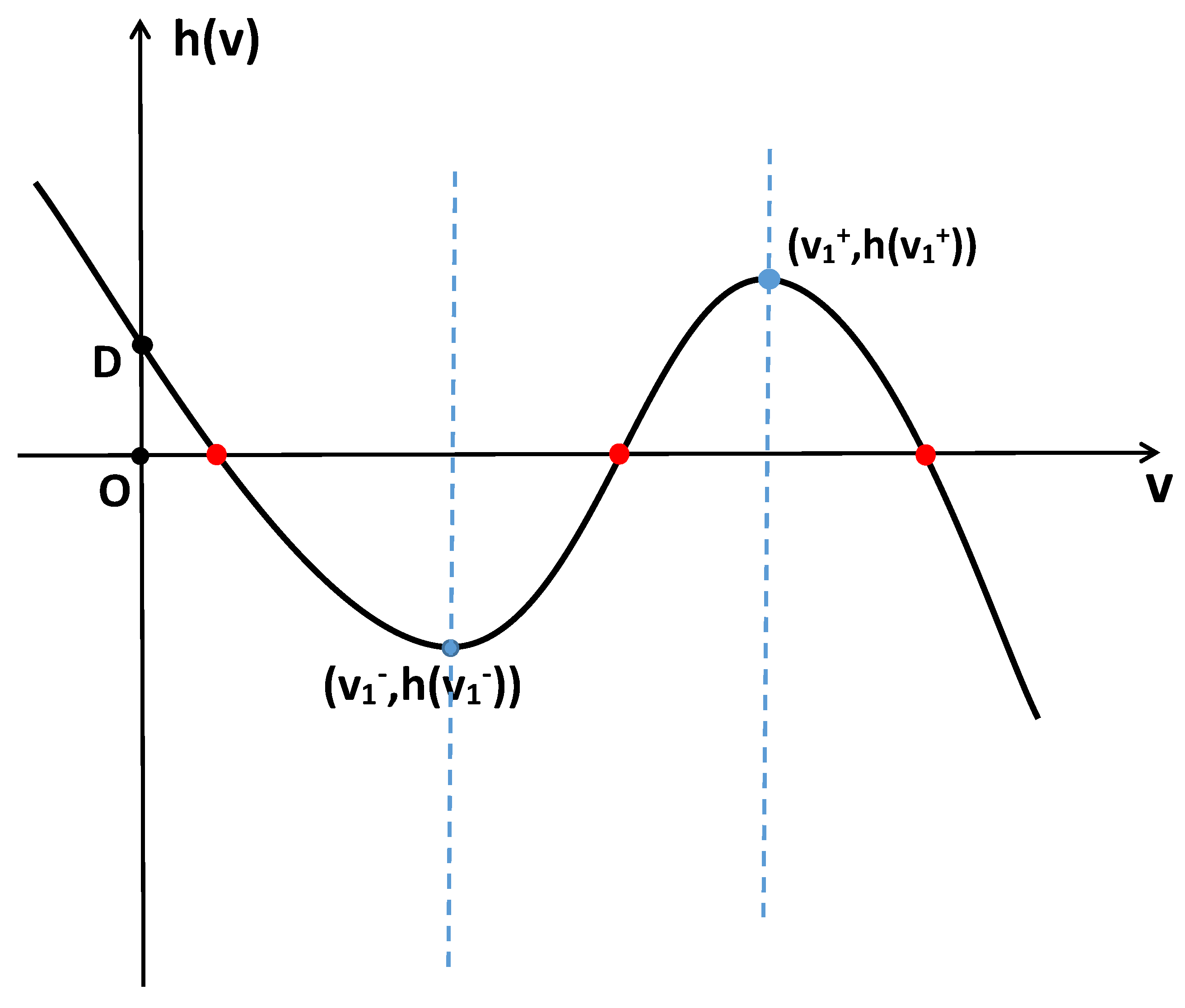
Figure 1.
If holds, then system (2) has three positive constant steady states.
Figure 1.
If holds, then system (2) has three positive constant steady states.

Figure 2.
System (2) has two positive constant steady states under various conditions. (a,b) Correspond to when holds. (c) Corresponds to when holds. (d) Corresponds to when holds.
Figure 2.
System (2) has two positive constant steady states under various conditions. (a,b) Correspond to when holds. (c) Corresponds to when holds. (d) Corresponds to when holds.

Figure 3.
System (2) has one positive constant steady state under various conditions. (a,b) Correspond to when holds. (c,d) Correspond to when holds. (e) Corresponds to when holds. (f) Left corresponds to when holds, and right corresponds to when holds.
Figure 3.
System (2) has one positive constant steady state under various conditions. (a,b) Correspond to when holds. (c,d) Correspond to when holds. (e) Corresponds to when holds. (f) Left corresponds to when holds, and right corresponds to when holds.

Figure 4.
Choose and the initial function is (). Then the positive constant steady state of system (2) is locally asymptotically stable.
Figure 4.
Choose and the initial function is (). Then the positive constant steady state of system (2) is locally asymptotically stable.

Figure 5.
Choose and consider the initial function as (, ). Then system (2) exhibits a spatially inhomogeneous stable periodic solution.
Figure 5.
Choose and consider the initial function as (, ). Then system (2) exhibits a spatially inhomogeneous stable periodic solution.

Figure 6.
Choose and consider the initial function as (, ). The constant steady state solution of system (2) is unstable.
Figure 6.
Choose and consider the initial function as (, ). The constant steady state solution of system (2) is unstable.

Figure 7.
Choose and the initial function is (, ). Then the constant steady state of system (1) is locally asymptotically stable.
Figure 7.
Choose and the initial function is (, ). Then the constant steady state of system (1) is locally asymptotically stable.

Figure 8.
Choose , and consider the initial function as (), then system (1) exhibits a spatially homogeneous stable periodic solution.
Figure 8.
Choose , and consider the initial function as (), then system (1) exhibits a spatially homogeneous stable periodic solution.

Disclaimer/Publisher’s Note: The statements, opinions and data contained in all publications are solely those of the individual author(s) and contributor(s) and not of MDPI and/or the editor(s). MDPI and/or the editor(s) disclaim responsibility for any injury to people or property resulting from any ideas, methods, instructions or products referred to in the content. |
© 2023 by the authors. Licensee MDPI, Basel, Switzerland. This article is an open access article distributed under the terms and conditions of the Creative Commons Attribution (CC BY) license (https://creativecommons.org/licenses/by/4.0/).
Share and Cite
MDPI and ACS Style
Xue, Y.; Xu, J.; Ding, Y. Spatiotemporal Dynamics of a Diffusive Immunosuppressive Infection Model with Nonlocal Competition and Crowley–Martin Functional Response. Axioms 2023, 12, 1085. https://doi.org/10.3390/axioms12121085
AMA Style
Xue Y, Xu J, Ding Y. Spatiotemporal Dynamics of a Diffusive Immunosuppressive Infection Model with Nonlocal Competition and Crowley–Martin Functional Response. Axioms. 2023; 12(12):1085. https://doi.org/10.3390/axioms12121085
Chicago/Turabian StyleXue, Yuan, Jinli Xu, and Yuting Ding. 2023. "Spatiotemporal Dynamics of a Diffusive Immunosuppressive Infection Model with Nonlocal Competition and Crowley–Martin Functional Response" Axioms 12, no. 12: 1085. https://doi.org/10.3390/axioms12121085
Note that from the first issue of 2016, this journal uses article numbers instead of page numbers. See further details here.