

Multi-Scale Reconstruction of Turbulent Rotating Flows with Generative Diffusion Models
by
 ,
,
Tianyi Li
1,
Alessandra S. Lanotte
2,*,
Michele Buzzicotti
1,
Fabio Bonaccorso
1 and
Luca Biferale
1 1
Department of Physics and INFN, University of Rome “Tor Vergata”, Via della Ricerca Scientifica 1, 00133 Rome, Italy
2
Istituto di Nanotecnologia, CNR NANOTEC and INFN, Via per Monteroni, 73100 Lecce, Italy
*
Author to whom correspondence should be addressed.
Atmosphere 2024, 15(1), 60; https://doi.org/10.3390/atmos15010060
Submission received: 29 November 2023
/
Revised: 27 December 2023
/
Accepted: 30 December 2023
/
Published: 31 December 2023
(This article belongs to the Special Issue Turbulence from Earth to Planets, Stars and Galaxies—Commemorative Issue Dedicated to the Memory of Jackson Rea Herring)
Abstract
:We address the problem of data augmentation in a rotating turbulence set-up, a paradigmatic challenge in geophysical applications. The goal is to reconstruct information in two-dimensional (2D) cuts of the three-dimensional flow fields, imagining spatial gaps present within each 2D observed slice. We evaluate the effectiveness of different data-driven tools, based on diffusion models (DMs), a state-of-the-art generative machine learning protocol, and generative adversarial networks (GANs), previously considered as the best-performing method both in terms of point-wise reconstruction and the statistical properties of the inferred velocity fields. We focus on two different DMs recently proposed in the specialized literature: (i) RePaint, based on a heuristic strategy to guide an unconditional DM for flow generation by using partial measurements data, and (ii) Palette, a conditional DM trained for the reconstruction task with paired measured and missing data. Systematic comparison shows that (i) DMs outperform the GAN in terms of the mean squared error and/or the statistical accuracy; (ii) Palette DM emerges as the most promising tool in terms of both point-wise and statistical metrics. An important property of DMs is their capacity for probabilistic reconstructions, providing a range of predictions based on the same measurements, enabling uncertainty quantification and risk assessment.
1. Introduction
In atmospheric and oceanic forecasting, the accurate estimation of systems from incomplete observations is a challenging task [1,2,3,4,5]. These environments, often characterized by turbulent dynamics, require effective reconstruction techniques to overcome the common problem of temporally or spatially gappy measurements. The challenge arises from factors such as instrument sensitivity, the natural sparsity of observational data, and the absence of direct information, for example, in the case of deeper ocean layers [6,7,8,9,10]. Established data assimilation techniques, such as variational methods [11,12] and ensemble Kalman filters [13,14], effectively merge time-series observations with model dynamics to attack the inverse problem. When measurements are limited to a single time point, gappy proper orthogonal decomposition (POD) [15] and extended POD [16] deal with spatially incomplete data by exploiting pretrained statistical relationships between measurements and missing information for the data augmentation goal. These POD-based methods are widely used in fluid mechanics [17,18,19] and geophysical fluid dynamics [20,21] to reconstruct flow fields.
POD-based methods are fundamentally linear, yielding reconstructions with smooth flow properties, associated with few leading POD modes. In the context of turbulent flows, this implies that POD-like methods primarily emphasize large-scale structures [22,23]. In recent years, machine learning has led to an increasing number of successful applications in reconstruction tasks for simple and idealized fluid mechanics problems (see [24] for a brief review). We refer to super-resolution applications (i.e., finding high-resolution flow fields from low-resolution data) [25,26,27], inpainting (i.e., reconstructing flow fields having spatial damages) [23,28], and inferring volumetric flows from surface or two-dimensional (2D)-section measurements [29,30,31]. However, much remains to be clarified concerning benchmarks and challenges, and this is even more important for realistic turbulent set-up and at increasing flow complexity, e.g., for increasing Reynolds numbers. When dealing with turbulent systems, the quality of reconstruction tasks must be judged according to two different objectives: (i) the point-wise error, given by the success in filling gappy or damaged regions of the instantaneous fields with data close to the ground truth configuration by configuration; (ii) statistical error, by reproducing statistical multi-scale and multi-point properties, such as the probability distribution functions (PDFs), spectra, etc., of the system.
To move from proof-of-concept to quantitative benchmarks, in a previous work [23], we systematically compared POD-based methods with generative adversarial networks (GANs) [32] using both point-wise and statistical reconstruction objectives for fully developed rotating turbulent flows, accounting for different gap sizes and geometries. GANs belong to the large family of generative models, i.e., machine learning algorithms that produce data according to a probability distribution optimized to resemble that of the data used in the training. The learning task is produced by two networks that compete with each other: First, a generative network is used to predict the data in the gap from the input measurement to obtain a good point-wise reconstruction. Second, to overcome the lack of expressiveness in the multi-scale (with low energetic content) flow structures, a second adversarial network, called the discriminator, is used to optimize the statistical properties of the generated data. Contrary to expectations, despite their non-linearity, GANs only matched the best linear POD techniques in point-wise reconstruction. However, GANs showed superior performance in capturing the statistical multi-scale non-Gaussian fluctuation characteristics of three-dimensional (3D) turbulent flow [23].
From our previous comparative study, we also observed that GANs pose many challenges in the training processes, due to the presence of instability and the necessity for hyper-parameter fine-tuning to achieve a suitable compromise in the multi-objective task. Furthermore, a common limitation of our GANs and POD-based methods is that they provide only a deterministic reconstruction solution. This singular output contrasts with the intrinsic nature of turbulence reconstruction, which is a one-to-many problem with multiple plausible solutions. The ability to generate an ensemble of possible reconstructions is critical for practical atmospheric and oceanic forecasting, e.g., in relation to uncertainty quantification and the risk assessment of rare, high-impact events [33,34,35].
More recently, diffusion models (DMs) [36] have emerged as a powerful generative tool, showing exceptional success in domains such as computer vision [36,37,38], audio synthesis [39], and natural language processing [40], particularly outperforming GANs in image synthesis [38]. Their applications have also extended to fluid dynamics for super-resolution [41], flow prediction [42], and Lagrangian trajectory generation [43]. By introducing Markov chains to effectively generate data samples (see Section 2.2), the implementation of DMs eliminates the need to resort to the less stable adversarial training of GANs, making DMs generally more stable in the training stage. Another characteristic of DMs is their inherent stochasticity in the generation process, which allows them to produce multiple outputs that adhere to the learned distribution conditioned on the same input.
This study is the first attempt to use state-of-the-art generative DMs for the reconstruction of 2D velocity fields of rotating turbulence, a complex system characterized by both large-scale vortices and highly non-Gaussian and intermittent small-scale fluctuations [44,45,46,47,48]. This novel application of DMs provides a quantitative estimation of their effectiveness in the context of turbulent flows. Our objectives are twofold: first, we aim to make comprehensive comparisons with the best-performing GAN methods from our previous research, and second, we aim to investigate the effectiveness of DMs in probabilistic reconstruction tasks. The statistical description of rotating and/or stratified turbulence is a fundamental problem for atmospheric and oceanic flows, particularly when the rotation is strong enough and the quasi-geostrophic approximation can be applied. Jack Herring made key contributions in this field, by pioneering not only the application of closure theories to understand the behavior of turbulent motions in the two ranges of scales smaller and larger than those of the energy source [49,50], but also numerical simulations where the inverse energy transfer towards large scales was observed [51]. Our study deals with the complex description and reconstruction of the interplay of 3D almost-isotropic small-scale fluctuations with an approximate 2D large-scale flow.
The paper is organized as follows: In Section 2, we introduce the system under consideration and the two adopted strategies for flow reconstruction using DMs. The first is a heuristic conditioning method applied to an unconditional DM designed for flow generation, as demonstrated by RePaint [52]. The second strategy uses a supervised approach, training a DM conditioned on measurements, similar to the Palette method [53,54]. In Section 3, we discuss the performance of the two DMs in point-wise and statistical property reconstruction, in comparison with the previously analyzed GAN method [22]. In Section 4, we study the probabilistic reconstruction capacity of the DMs. We end with some comments in Section 5.
2. Methods
2.1. Problem Setup and Data Preparation
In this study, we focus on rotating turbulence [55,56], which is of considerable physical interest to geophysical and astrophysical problems [57,58]. Under strong rotation, the flow tends to become quasi-2D, characterized by the formation of large-scale coherent vortical structures parallel to the rotation axis [47]. We adopt the same experimental framework as our previous work [23], and explore possible improvements from DMs. We set up a mock field-measurement, anticipating being able to obtain data from a gappy 2D slice of the original 3D volume of rotating turbulence, orthogonal to the axis of rotation. The full 2D image is denoted as , the support of the measured domain as , and the support of the gap where we miss the data as . Here, represents a centrally located square gap of variable size, as shown in Figure 1a. We use the TURB-Rot database [59] obtained from direct numerical simulation (DNS) of the incompressible Navier–Stokes equations for rotating fluid in a 3D periodic domain, which can be written as
where is the incompressible velocity, is the rotation vector, and represents the pressure modified by a centrifugal term. The regular, cubic grid has points. The statistically homogeneous and isotropic forcing acts at large scales around , and it is the solution of a second-order Ornstein–Uhlenbeck process [60,61]. In the stationary state, with , the Rossby number is , where represents the kinetic energy. The viscous dissipation is replaced by a hyperviscous term to increase the inertial range, while a large-scale linear friction term is added to the r.h.s. of Equation (1) to reduce the formation of a large-scale condensate [46], associated with the inverse energy cascade well-developed at this Rossby number. The Kolmogorov dissipative wavenumber, , is chosen as the scale at which the energy spectrum begins to decay exponentially. An effective Reynolds number is defined as , with the smallest wavenumber . The integral length scale is , where is the domain length, and the integral time scale is . For further details of DNS, see [59]; a sketch of the original 2D spectrum is also shown in Figure 1b.
Data were extracted from the DNS by sampling the full 3D velocity field (Figure 1a) during the stationary stage at intervals of to reduce temporal correlation. We collected 600 early snapshots for training and 160 later snapshots for testing, with the two collections separated by over to ensure independence. To manage the data volume while preserving complexity, the resolution of the sampled fields was reduced from to using Galerkin truncation in Fourier space, with the truncation wavenumber set to . We then selected - planes at different -levels and augmented them by random shifts with the periodic boundary conditions, resulting in a train/test split of 84,480/20,480 samples.
For a baseline comparison, we use the best-performing GAN tailored for this setup in [23], which showed point-wise error close to the best POD-based method and good multi-scale statistical properties. In our analyses, we focus only on the velocity magnitude, . Briefly, the GAN framework consists of two competing convolutional neural networks: the first network is a generator that transforms input measurements into predictions for the missing or damaged data; the second is a discriminator that works to discriminate between generated data and real fields. The training of the generator minimizes a loss function consisting of the mean squared error (MSE) and an adversarial loss provided by the discriminator, optimizing point-wise accuracy and statistical fidelity, respectively. A more detailed description of the GAN can be found in [23].
2.2. DM Framework for Flow Field Generation
Before moving to the more difficult task to inpaint a gap conditioned on some partial measurements of each given image, we need to define how to generate unconditional flow realizations. Unlike GANs, which map input noise to outputs in a single step, DMs use a Markov chain to incrementally denoise and generate information through a neural network (see Figure 1c for a qualitative visual example of one generation event). This finer-grained framework, coupled with an explicit log-likelihood training objective, tends to yield more stable training than the tailored loss functions of GANs, but still has the capability of generating realistic samples. Another feature of DMs is their inherent stochasticity in the generation process, which allows them to produce multiple outputs that adhere to the learned distribution conditioned on the same input.
In this section, we introduce the DM framework for flow field generation. The velocity magnitude field on the full 2D domain is denoted by , and the distribution of this field is represented as . In order to train the model, we need first to produce a set of images with larger and larger noise. To do that, the DM framework defines a forward process or diffusion process that incrementally adds Gaussian noise to the data until they become indistinguishable from white noise after N diffusion steps (Figure 2).
This set of diffused images is used for training a network to perform a backward denoising process, starting from the set of pure i.i.d. Gaussian-noise 2D realizations and seeking to reproduce the set of images in the training dataset. Once the training is accomplished, the parameters of the network are frozen and used to generate brand new images by sampling from any realization of pure random images in the input (see Figure 3a for a sketch summary). The forward diffusion process is expressed in terms of a sequence of N steps, conditioned on the original set of images, i.e., for each image in the training dataset, we produce N noisy copies with an increasing amount of diffusion:
where is the initial magnitude field and represents the final white-noise state, an ensemble of Gaussian images made of uncorrelated pixels with zero mean and unit variance. The notation is used to denote the entire sequence of generated noisy fields, .
Each step, , of the forward process can be directly obtained as
which implies sampling from a Gaussian distribution where the mean of is given by and the variance is . The variance schedule is predefined to allow a continuous transition to the pure Gaussian state. For more details on the variance schedule and other aspects of the DMs used in this study, see Appendix B.
The DM trains a neural network to approximate the reverse process of Equation (3), denoted as . This approximation allows the generation of new velocity magnitude fields from Gaussian noise, , through a backward process (see Figure 3a) described by
where it is important to notice that the stochasticity in the process allows for the production of different final images even when starting from the same noise. In the continuous diffusion limit, characterized by sequences of small values of , the backward process has a functional form identical to that of the forward process, as discussed in [63,64]. Consequently, the neural network is tasked with predicting the mean and covariance of a Gaussian distribution:
The neural network is optimized to minimize an upper bound of the negative log likelihood,
This training objective tends to result in more stable training compared to the tailored loss functions used in GANs. For a detailed derivation of the loss function and insights into the training details, please refer to Appendix A.
2.3. Flow Field Data Augmentation with DMs: RePaint and Palette Strategies
RePaint. The RePaint approach aims to reconstruct missing information in the flow field using a DM that has been trained to generate the full 2D flow field from Gaussian noise, as described in the section above, without any conditioning on the measured data, and without relying on any further model training. To achieve the correct reconstruction, RePaint aims to ensure the conditioning on the measurements only by redesigning an ad hoc generation protocol [52]. As discussed above, during training, DM learns to approximate the backward transition probability to step on a sample , only from the knowledge of the sample obtained in the previous step ; hence, DM models the one-step backward transition probability, . The goal of RePaint is to set up a generative process where this backward probability is also conditioned on some measured data, denoted as . In this way, each new sample in the backward direction is generated from the one-step backward conditioned probability, defined as . To achieve this goal, RePaint substitutes the DM model input, , with another 2D field, , which is given by the union of projected only to have support inside the gap and the measured data on the support propagated at step n according to the forward process, namely, . In summary, at any generic backward step n, RePaint approximates the conditional backward probability as follows:
Here, represents the projection of the sample generated by the backward process at step n projected inside the gap region (the central square), while is the noisy version of the measured data (outside the square gap) that are obtained by a forward propagation up to step n of the measurements. At this point, , replacing , is given as input to the model and it is used to obtain the next sample at step , (see Figure 3c).
The propagation of information from the measurements into the gap happens thanks to the application of the non-linear (and non-local) function approximated by the U-Net employed in the DM. Hence, the output of the U-Net, describing the probability of moving from step n to , is the result of non-local convolutions mixing information in the two regions and . In this way, the model mitigates the discontinuities generated across the gap by merging the generated and the measured data. Furthermore, to allow a deeper propagation of information, improving correlations between the measurements and the generated data, RePaint employs a resampling strategy [52]. The idea of resampling, as shown schematically in Figure 3d, is that each sample at step , extracted from the conditioned probability, , is not directly used as input to move backward at step , but, instead, it is first propagated forward for j steps (by adding more noise) before returning according to the conditioned backward process at step . This operation gives the U-Net model the opportunity to iterate the propagation of information from the measured region inside the gap. Resampling can be applied at different steps multiple times, resulting in a back-and-forth progression during the generation process, as opposed to a monotonic backward progression from to . Further details, such as the network architecture and other parameters, can be found in Appendix B. As demonstrated in computer vision applications [52,65,66,67], this strategy has the advantage of being easily generalizable to diverse tasks, such as free-form inpainting with arbitrary mask shapes. However, this introduces several new challenges in the design of such a convoluted generation protocol, which is neither trivial in its optimization nor in its implementation.
Palette. An alternative approach to perform flow field reconstruction is to train the DM directly to learn the backward probability distribution conditioned on the measured data, previously introduced as . This method, called Palette, has been successfully used in various computer vision applications, such as image-to-image translation tasks [53,54]. The idea is to train a U-Net using the same strategy as any unconditioned DM, but giving the network as input the additional information coming from the measurements, at any step during the diffusion process. This allows the model to learn during training how to use information from the available data to achieve optimal reconstruction inside the gap. In addition, unlike the RePaint method, Palette always uses the measured data without adding noise. In this way, the forward process can be defined as for the pure generation case, but it takes place only within the gap region, while the data on the support, , are frozen throughout the diffusion process and serve as an additional input to the model. A schematic summary of the Palette approach is shown in Figure 4. Once the DM model is trained, since the reconstruction process is Markovian as in the standard generative DM, the conditional probability of the reconstructed field, , can be determined through the following iterative process:
starting from any Gaussian noise . To facilitate the comparison with the GAN model implemented in our previous works [23,28], we trained a separate Palette model for each fixed mask size. Let us stress that both methods are capable of training on a free-form mask [68]. More details on Palette are provided in Appendix B.
3. Comparative Analysis of DMs and the GAN in Flow Reconstruction
To provide a systematic comparison between DMs and the GAN in flow reconstruction, we focus on cases where the 2D velocity magnitude fields have a central square gap of variable size, spanning , where is the size of the whole flow domain. In this section, only one reconstruction realization is performed for all the image data in the testing ensemble, i.e., we do not further explore the possibility of assessing the robustness of the prediction by sampling over the ensemble of predicted images (see next section). The initial evaluation focuses on the reconstructed single-point velocity magnitude, which is strongly influenced by large-scale coherent structures. Then, we analyze the reconstruction process from a multi-scale perspective by examining the statistical properties of the gradient of the reconstructed velocity magnitude and by looking at other scale-dependent statistics in both real and Fourier space.
3.1. Large-Scale Information
To quantify the reconstruction error between the predicted velocity magnitude, , and the true velocity magnitude, , within the gap region, we introduce the normalized MSE as follows:
Here, represents the spatially averaged error in the central, gappy region for a single-flow configuration, and it is calculated as
where denotes the area of the gap. Averaging is performed over the test dataset. The normalization factor, , is defined as the product of the standard deviations of the predicted and true velocity magnitudes within the gap:
where
and is similarly defined. This choice for the normalization term, , ensures that predictions with significantly low or high energy levels will result in a large MSE.
In our analysis, we use the Jensen–Shannon (JS) divergence to assess the distance between the PDF of a predicted quantity and the PDF of the true data. Specifically, the JS divergence applied to two distributions and defined on the same sample space is
where and
is the Kullback–Leibler (KL) divergence. As the two distributions get closer, the value of the JS divergence becomes smaller, with a value of zero indicating that P and Q are identical.
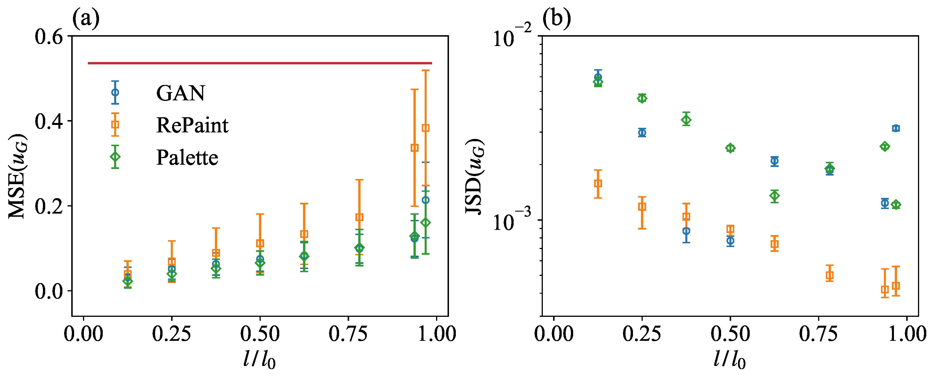
Figure 5a shows the as a function of the normalized gap size, . It shows that Palette achieves a comparable MSE with respect to GAN for most gap sizes. Only for the largest gap size, , is the MSE of Palette significantly better than that of GAN. On the other hand, RePaint has a larger MSE for all sizes compared to the other two methods, demonstrating the limitations of the RePaint approach in enforcing correlations between the measurements and generated data without being specifically trained on a reconstruction problem, as in the other two approaches. The red baseline, derived from predictions using randomly shuffled test data, represents the case where the predictions guess the exact statistical properties, and , but lose all correlation with the measurements, .
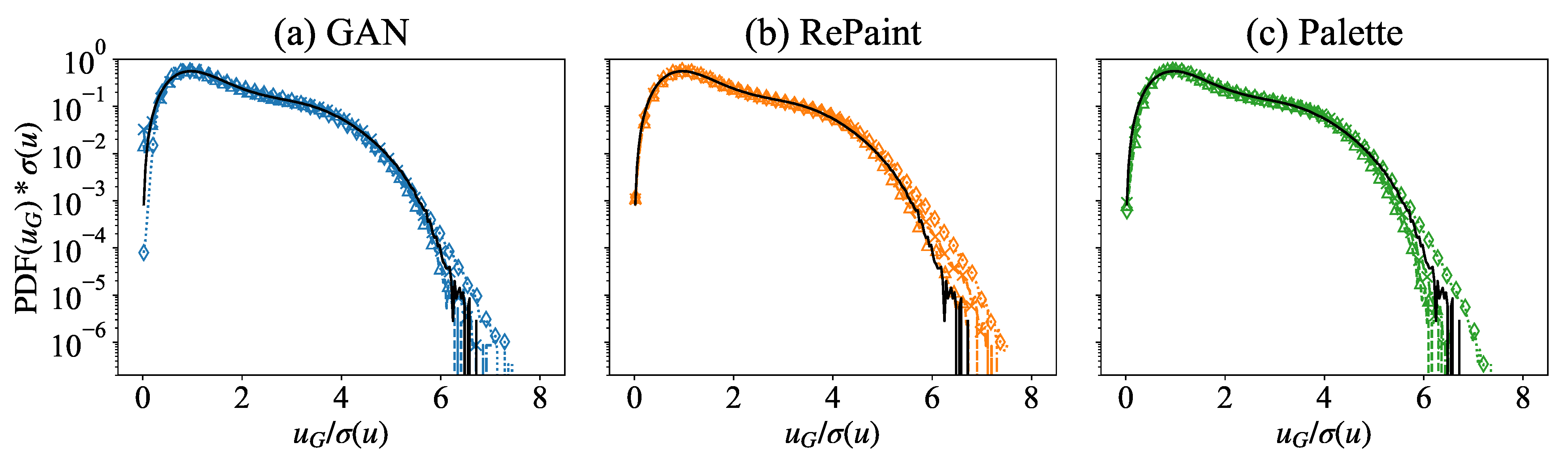
We now examine the velocity magnitude PDFs as predicted by the different methods and compare them with the true data. In Figure 5b, we present the JS divergence between the predicted and true velocity magnitudes, denoted as . First of all, it is important to highlight that all the values are well below , suggesting that there is always a close match between the PDFs of the reconstructed and of the true velocity magnitude. The agreement between the different PDFs is also shown in Figure 6, where one can see the extremely good performance of all models in closely matching the PDFs of the generated velocity magnitude with the ground truth one. Going back to the results presented in Figure 5b, it is possible to note that in the small gap region, , there is a monotonic behavior of the JS divergence, which tends to decrease as the gap increases. This can be interpreted by the fact that the main contribution to the JS divergence is due to statistical fluctuations in the PDF tails which are less accurately estimated when the gap is small. This behavior is clearly visible in the results of the RePaint approach, which shows a monotonic decrease in the JS divergence over the whole range of gaps analyzed. The same effect is not visible in the other approaches in the range above . The reason is probably that both GAN and Palette rely on different training to reconstruct different gap sizes, and the fluctuations due to the training convergence could be underestimated. The non-monotonicity is much more pronounced in the GAN results as this approach is known to be less stable during training. The analysis shows that, compared to the other two approaches, RePaint trained on the pure generation without any conditioning is the best method to obtain a statistical representation of the true data.
In Figure 7, we compare the PDFs of the spatially averaged error, , for different flow configurations. For small and medium gap sizes (Figure 7a,b), the PDFs of GAN and Palette closely match, whereas the PDF of RePaint, although similar in shape, exhibits a range with larger errors. For the largest gap size (Figure 7c), Palette is clearly the most accurate, predicting the smallest errors. Again, RePaint performs the worst, characterized by a peak at high error values and a broad error range.
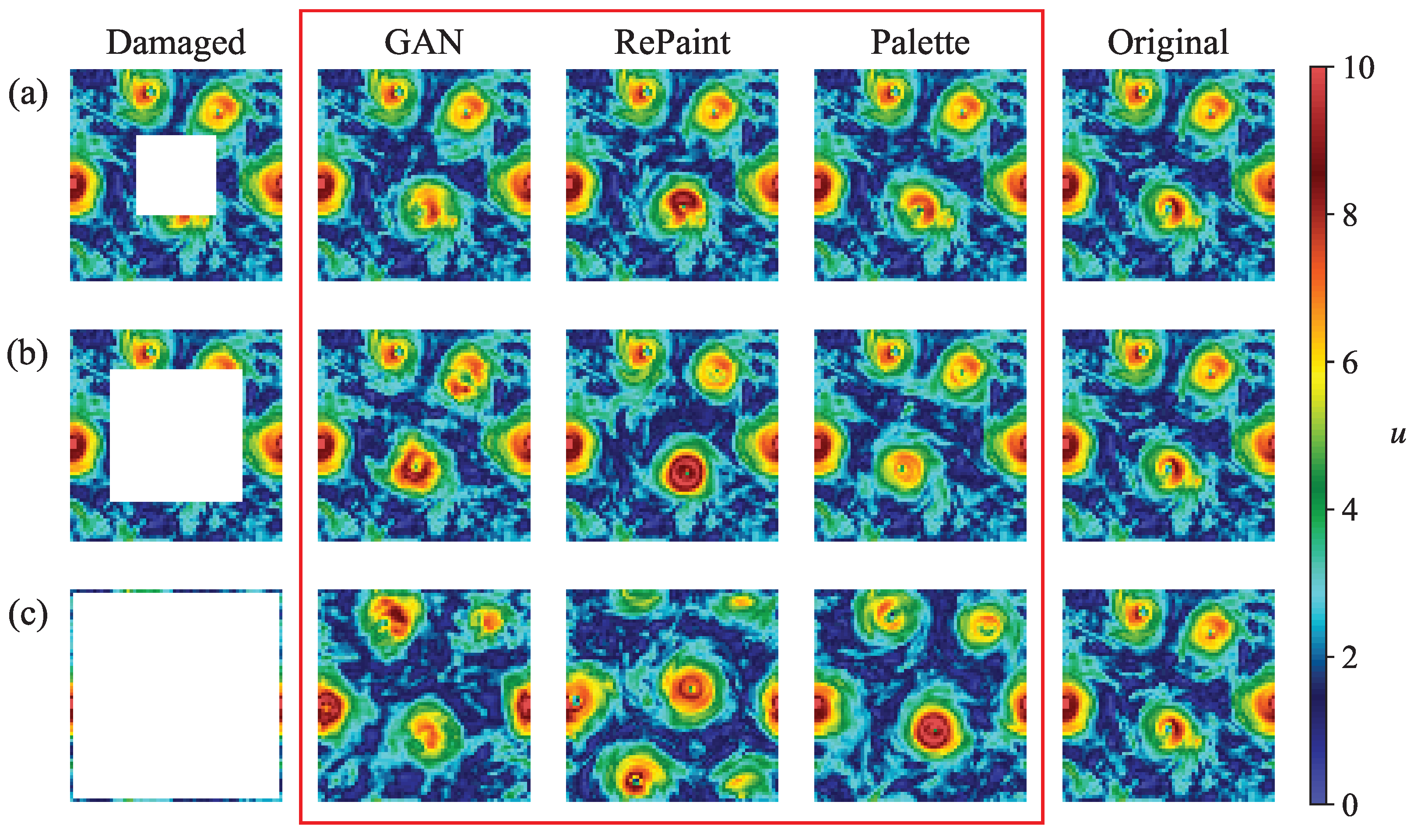
Finally, Figure 8 provides a visual qualitative idea of the reconstruction capabilities of the instantaneous velocity magnitude field using the three adopted models. While all methods generally perform well in locating vortex structures within smaller gaps and produce realistic turbulent reconstructions, RePaint is a notable exception. In particular, for the largest gap (in Figure 8c), RePaint’s performance lags significantly behind the other two methods, failing to accurately predict vortex positions and resulting in a significantly larger MSE.
3.2. Multi-Scale Information
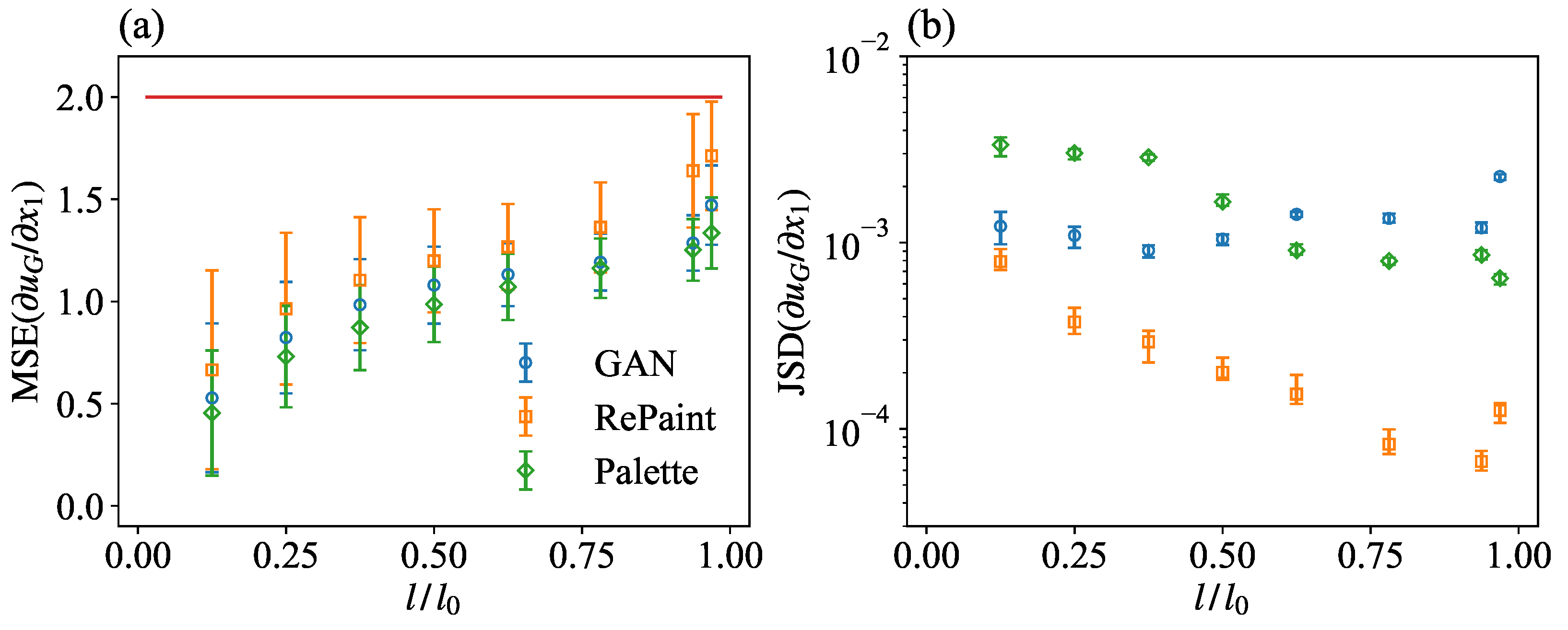
This section presents a quantitative analysis of the multi-scale information reconstructed by the different methods. We begin by examining the gradient of the reconstructed velocity magnitude in the missing region, denoted as . Figure 9a shows the MSE of this gradient, , defined similarly to Equation (9). The results show that Palette consistently achieves the lowest MSE. GAN’s performance is comparable for most gap sizes, but deteriorates significantly at the extremely large gap size. In contrast, while RePaint has larger point-wise reconstruction errors for the gradient, it maintains the smallest JS divergence, , as shown in Figure 9b, indicating its robust statistical properties.
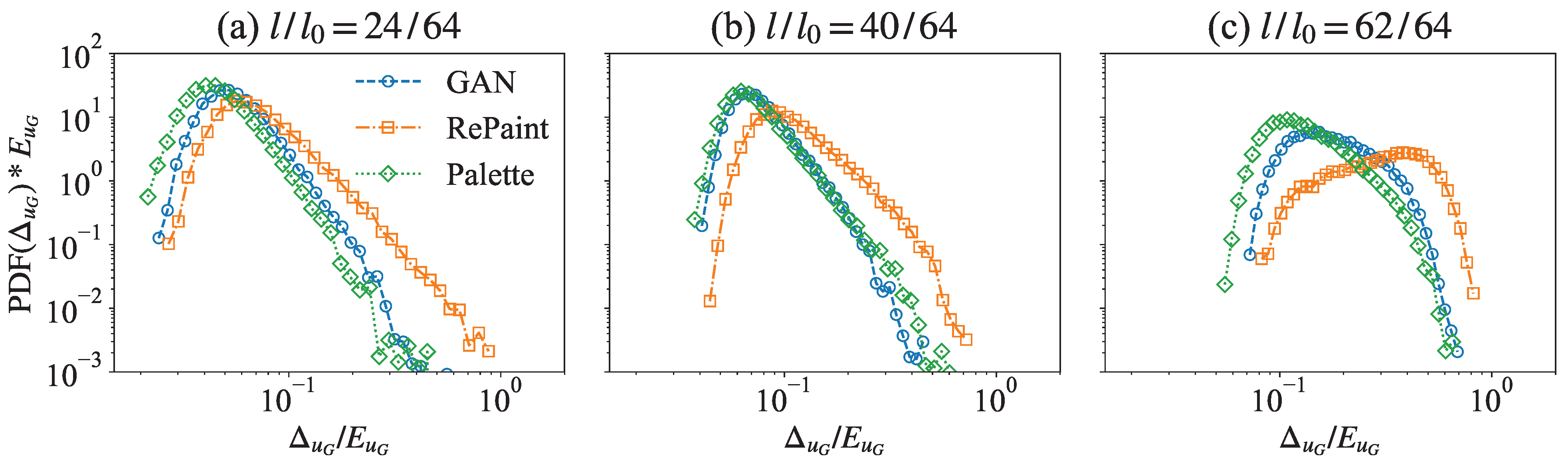
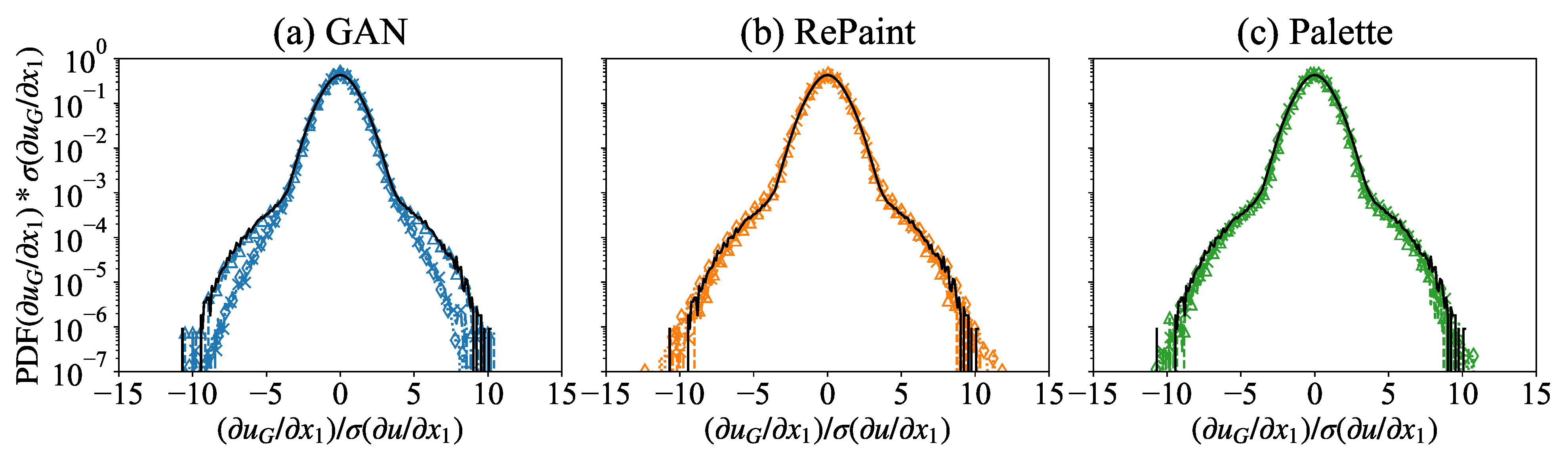
For small gap sizes, Palette has larger JS divergence than GAN, while the situation is reversed at higher gap values (Figure 9b). It is worth noting that, like the velocity module PDFs, the reconstructed gradient PDFs are very well matched by all three methods. In contrast to velocity, the GAN reconstruction is less accurate for very large gaps in the case of gradient statistics, as can be seen by comparing the PDFs in the different panels of Figure 10. This last observation limits the applications of the GAN to the modeling of small-scale turbulent observables.
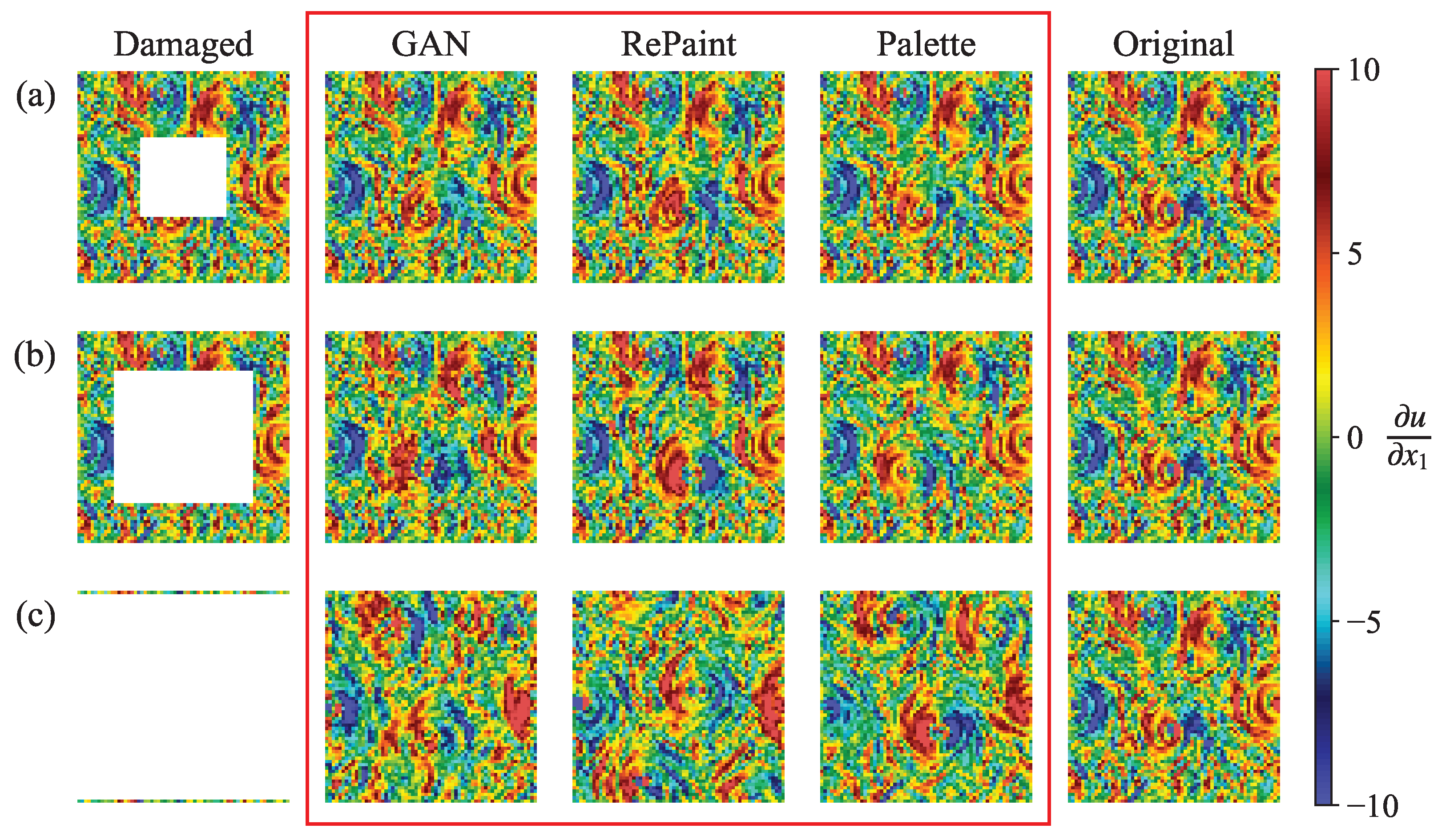
The results of these methods can be more directly visualized by examining the gradient of the reconstruction samples, as shown in Figure 11. For small gap sizes (Figure 11a), all three methods produce realistic predictions that correlate well with the original structure. However, for medium and large gap sizes (Figure 11b,c), only Palette is able to generate gradient structures that are well correlated with the ground truth.
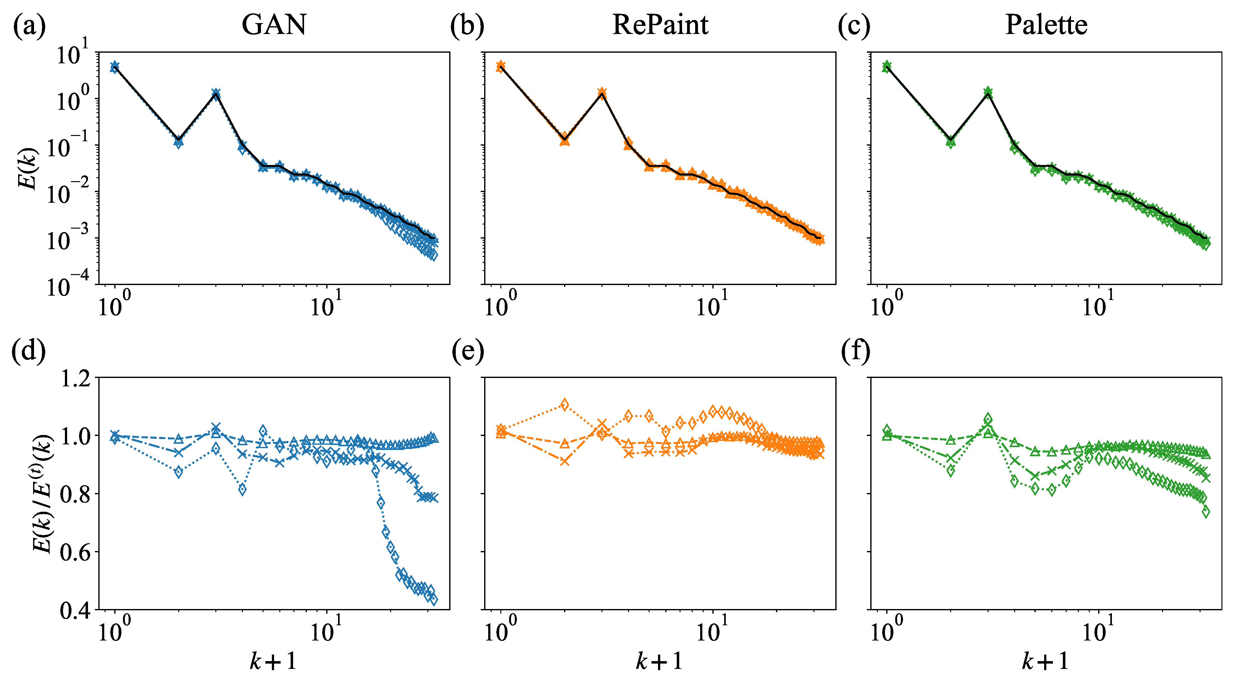
The better performance of DMs in capturing the statistical properties is further demonstrated by a scale-by-scale analysis of the 2D energy spectrum obtained from the reconstructed fields,
Here, denotes the horizontal wavenumber, is the Fourier transform of the velocity magnitude, and is its complex conjugate. Direct comparison of the spectra are shown in Figure 12a–c, for three gap sizes. In Figure 12d–f, we plot the ratio of the reconstructed to the original spectra, denoted as . Deviations from unity in this ratio better highlight the wavenumber regions where the reconstruction is less accurate. While all the methods produce satisfactory energy spectra, a closer examination of the ratio to the original energy spectrum shows that RePaint and Palette maintain uniformly good correspondence across all scales and for all gap sizes. Conversely, GAN performs well at small gap sizes, but exhibits poorer performance at large wavenumbers for medium and large gap sizes.
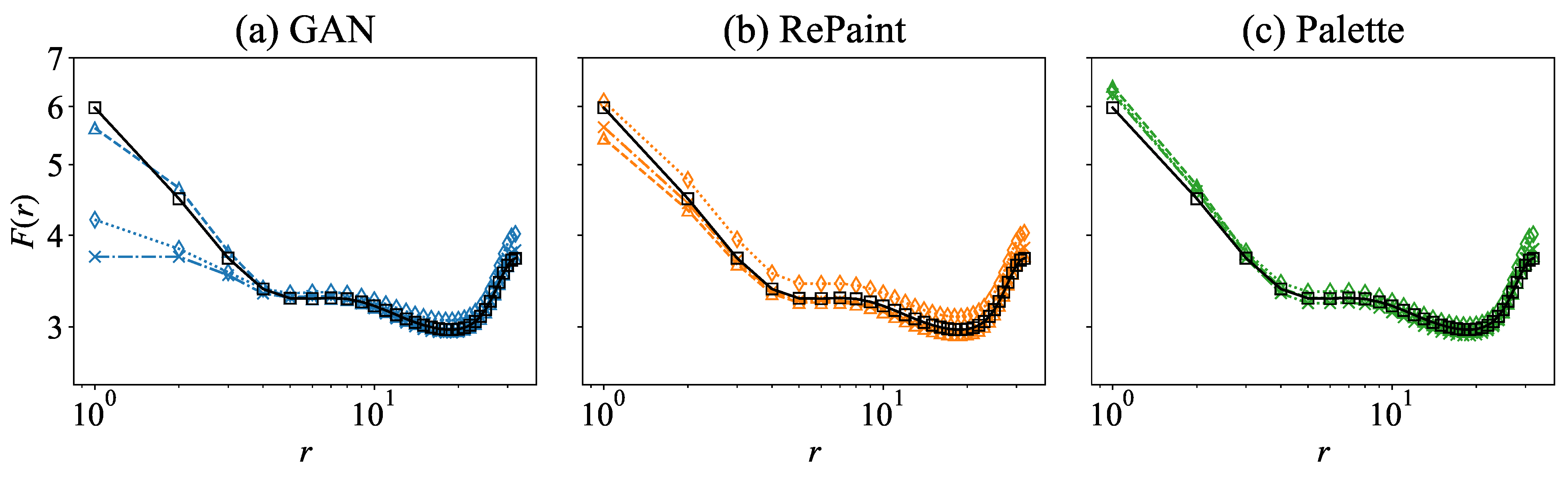
Consistent results are observed when examining the flatness of the velocity magnitude increments:
where and , with denoting the average over the test data and over , for points and , where only one, or both of them, are within the gap. The flatness calculated over the entire region of the original field is also shown for comparison. In Figure 13, the flatness results further confirm that RePaint and Palette consistently maintain their high-quality performance across all scales. In contrast, while GAN is effective at small gap sizes, it faces challenges in maintaining similar standards at small scales for medium and large gap sizes.
4. Probabilistic Reconstructions with DMs
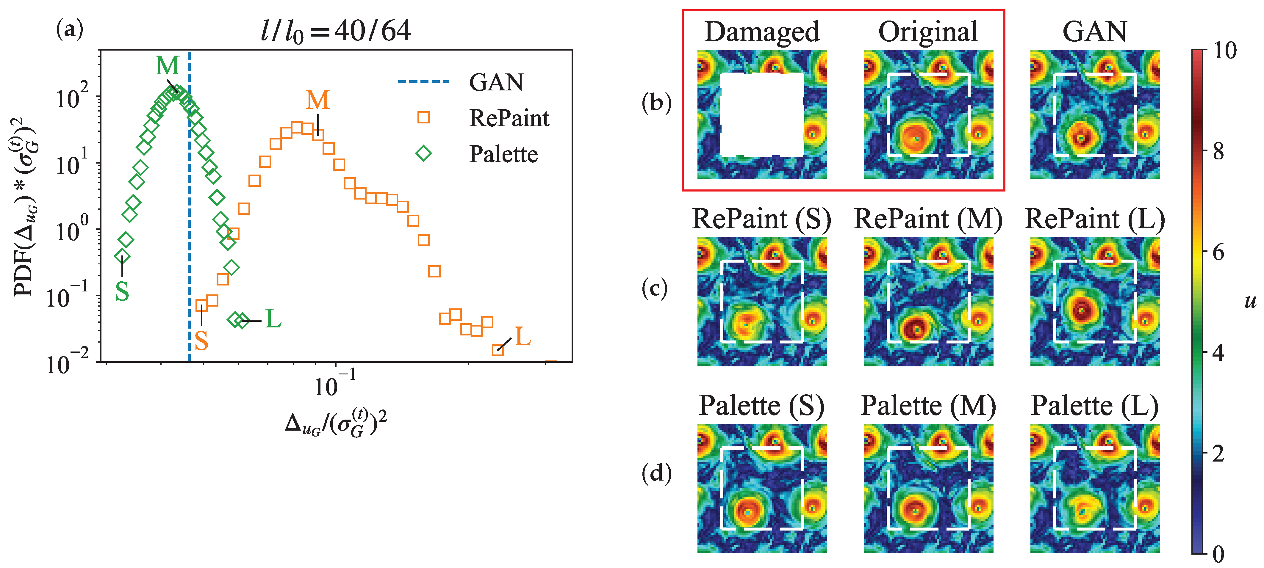
So far, we have analyzed the performances of the three models in the reconstruction of the velocity magnitude itself and its statistical properties. In this section, we explore the probabilistic reconstruction capabilities of DMs, i.e., the fact that DMs provide us with many possible reconstructions that we can quantify in terms of a mean error and a variance. This is a significant advantage over the GAN architecture we have used in this work. It is worth noting that the implementation of stochastic GANs is also possible, although not of interest for our analysis. Focusing on a specific gap size, we select two flow configurations: the first is a configuration for which the discrepancy between the reconstructed fields and the true data–as quantified by the mean error—is small and comparable across GAN, Palette, and RePaint; the second is a more complex situation for reconstruction, as all models display large discrepancies from the true data. For each of these two configurations, we performed 20,480 reconstructions using RePaint and Palette.
Figure 14a displays the PDFs of the spatially averaged errors across different reconstruction realizations, compared to GAN’s unique reconstruction error indicated by a blue dashed line. The comparison shows that Palette achieves a lower mean error than GAN, along with a smaller variance, indicating high model confidence for this case. In contrast, RePaint tends to produce higher errors with a wider variance. The comparison is more evident in Figure 14b, where it appears that GAN provides a realistic reconstruction with accurate vortex positioning. As for RePaint, it sometimes inaccurately predicts the vortex positions (Figure 14c (L)) or fails to accurately represent the energy distribution, even when the position is correct (Figure 14c (S) and (M)), leading to larger errors. Conversely, Figure 14d shows that Palette consistently predicts the correct position of vortex structures, with variations in vortex shape or energy distribution being the primary factors affecting the narrow reconstruction error distribution.
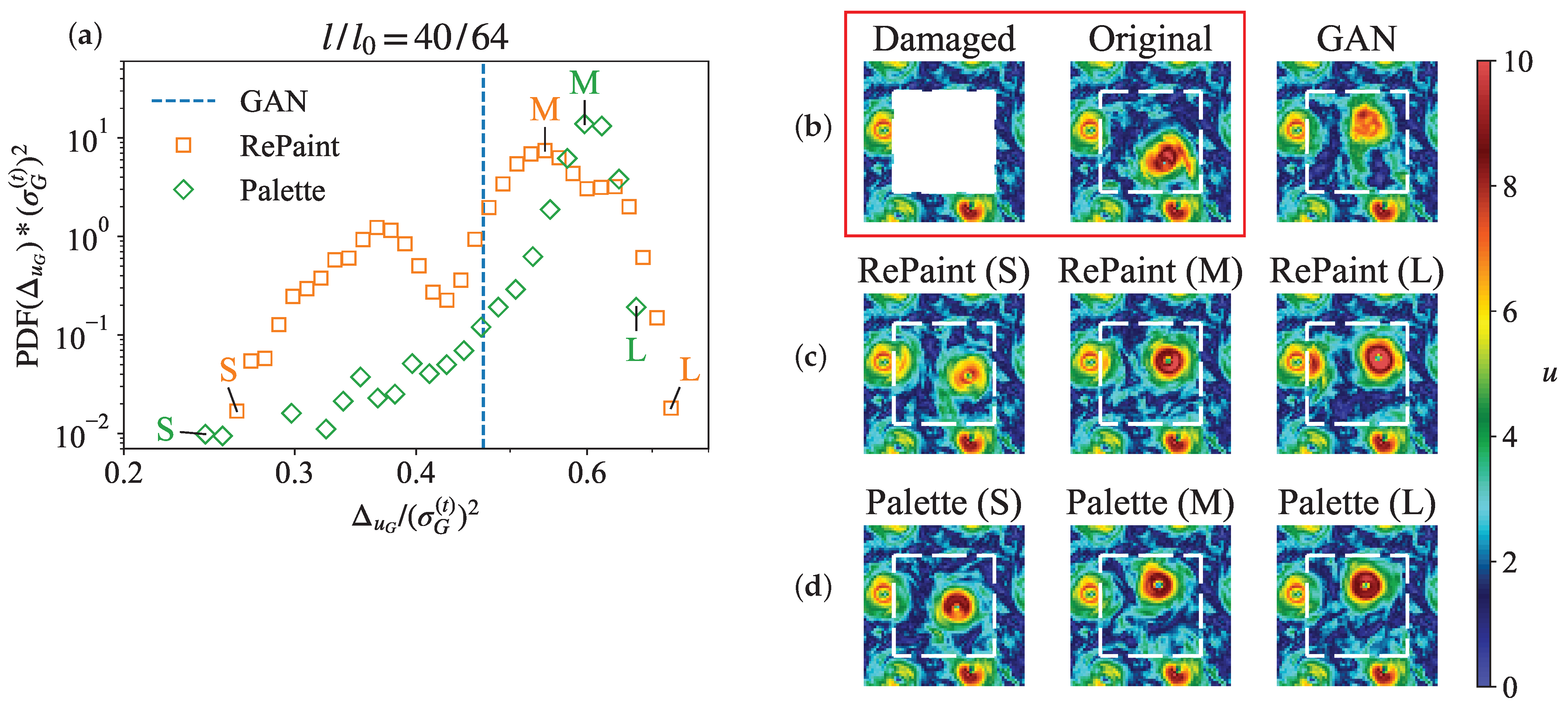
Figure 15 presents the same evaluations for the configuration where all models produce large errors. As shown in Figure 15a, both RePaint and Palette show significant variance in errors, with their mean errors exceeding that of GAN. The ground truth, examined in Figure 15b, highlights the inherent difficulty of this reconstruction scenario. In particular, an entire vortex structure is missing, and the proximity of two strong vortices suggests a potential transient state, possibly involving vortex merging or vortex breakdown. These situations may be rare in the training data, leading to a complete failure of GAN to accurately predict the correct vortex position, as shown in Figure 15b. For RePaint, the challenge of this reconstruction is reflected in the different predictions of the vortex positions. While some of these predictions are more accurate than GAN’s, RePaint also tends to produce incoherence around the gap boundaries (Figure 15c). Conversely, Figure 15d shows that Palette’s predictions are not only more consistent with the measurements, but also provide a range of reconstructions with different vortex positions.
5. Conclusions and Discussion
In this study, we investigated the data augmentation ability of DMs for damaged measurements of 2D snapshots of a 3D rotating turbulence at moderate Reynolds numbers. The Rossby number is chosen such as to produce a bidirectional energy cascade at both large and small scales. Two DM reconstruction methods are investigated: RePaint, which uses a heuristic strategy to guide an unconditional DM in the flow generation, and Palette, a conditional DM trained with paired measurements and missing information. As a benchmark, we compared these two DMs with the best-performing GAN method on the same dataset. We showed that there exists a trade-off between obtaining a reliable error and good statistical reconstruction properties. Typically, models that are very good for the former are less accurate for the latter. Overall, according to our analysis, Palette seems to be the most promising tool considering both metrics. Indeed, our comparative study shows that while RePaint consistently exhibits superior statistical reconstruction properties, it does not achieve small errors. Conversely, Palette achieves the smallest errors along with very good statistical results. Moreover, we observe that GAN fails to provide statistical properties that are as accurate as the DMs at small scales for medium and large gaps.
Concerning probabilistic reconstructions, a crucial feature for turbulent studies and uncertainty quantification for both theoretical and practical applications, we evaluated the effectiveness of the two DM methods on two specific configurations of different complexity. For the configuration with sufficient information in the measurement, Palette shows errors that tend to be smaller than GAN and exhibits a small variance, indicating high model confidence. However, RePaint faces challenges in accurately predicting large-scale vortex positions and struggles to achieve an accurate energy distribution. This difficulty partly stems from RePaint’s heuristic conditioning strategy, which cannot effectively guide the generative process using the measurement. In a more complex scenario characterized by the presence in the gappy region of an entire large-scale structure, GAN completely fails to predict the correct vortex position, while both DMs can localize it with higher precision by taking advantage of multiple predictions, although RePaint shows incoherence around the gap boundaries.
In summary, this study establishes a new state-of-the-art method for the 2D snapshot reconstruction of 3D rotating turbulence using conditional DMs, surpassing the previous GAN-based approach. The better performance of DMs over GANs stems from their iterative, denoising construction process, which builds up the prediction scale-by-scale, resulting in better performance across all scales. The inherent stochasticity of this iterative process yields a probabilistic set of predictions conditioned on the measurement, in contrast to the unique prediction of the GAN implemented here. Our study opens the way to further applications for risk assessment of extreme events and in support of various data assimilation methods. It is important to note that DMs are significantly more computationally expensive than GANs due to the iterative inference steps. Despite this, many efforts in the computer vision field have been devoted to accelerating this process [69,70].
A promising avenue for future studies could focus on flows at higher Reynolds numbers and Rossby numbers, close to the critical transition, leading to the inverse energy cascade, a very complex turbulent situation where both 3D and 2D physics coexist in a multi-scale environment. In addition, it would be interesting to test our method in practical scenarios, such as wind farm flows [71,72,73], where it could potentially help to synthesize inflow conditions and reconstruct the associated dynamics. The present work focuses on cases where only instantaneous measurements are available, without temporal sequences. In the future, machine learning methods, such as long short-term memory (LSTM) [74] and transformer [75], could be used to exploit temporal correlations.
Author Contributions
All authors contributed to the conceptualization and to the writing of the results. T.L. and M.B. contributed to the development of the methodology, A.S.L. and L.B. to the formal analysis, and F.B. to the curation of the data and software. All authors have read and agreed to the published version of the manuscript.
Funding
This research was funded by the European Research Council (ERC) under the European Union’s Horizon 2020 research and innovation programme, grant agreement number 882340 and by the EHPC-REG-2021R0049 grant. ASL received partial financial support from ICSC—Centro Nazionale di Ricerca in High Performance Computing, Big Data, and Quantum Computing, funded by the European Union—NextGenerationEU. LB and MB received partial funding from the program FARE-MUR R2045J8XAW. MB acknowledges the hospitality of the Eindhoven University of Technology TUe, where part of this work was carried out.
Institutional Review Board Statement
Not applicable.
Informed Consent Statement
Not applicable.
Data Availability Statement
The 2D snapshots of velocity data from rotating turbulence used in this study are openly available on the open-access Smart-TURB portal (http://smart-turb.roma2.infn.it) (access date: 14 June 2020), under the TURB-Rot repository [59]. The codebase for the two DM reconstruction methods, RePaint and Palette, is available at https://github.com/SmartTURB/repaint-turb (access date: 23 November 2023) and https://github.com/SmartTURB/palette-turb (access date: 16 November 2023), respectively.
Conflicts of Interest
The authors declare no conflicts of interest.
Abbreviations
The following abbreviations are used in this manuscript:
| 2D | Two-dimensional |
| DM | Diffusion model |
| GAN | Generative adversarial network |
| POD | Proper orthogonal decomposition |
| Probability density function | |
| 3D | Three-dimensional |
| DNS | Direct numerical simulation |
| MSE | Mean squared error |
| JS | Jensen–Shannon |
| KL | Kullback–Leibler |
Appendix A. Training Objective of DM for Flow Field Generation
A notable property of the forward process is that it allows closed-form sampling of at any given diffusion step n [76]. With definitions of and , we have
Specifically, for any real flow field , we can directly evaluate its state after n diffusion steps using
where .
To optimize the negative log likelihood, , which is numerically intractable, we focus on optimizing its usual variational bound:
The objective can be further reformulated as a combination of KL divergences, denoted as , plus an additional entropy term [36,64]:
The first term, , has no learnable parameters as is a Gaussian distribution, and can, therefore, be ignored during training. The terms within the second part of the summation, , represent the KL divergence between and the posteriors of the forward process conditioned on , which are tractable using Bayes’ theorem [43,76]:
where
and
By setting to untrained constants, where can be either or , as discussed in [36], the KL divergence between the two Gaussians in Equations (3) and (5) can be expressed as
Given the Gaussian form of as presented in Equation (5), the term also results in the same form as Equation (A8). Substituting Equation (A2) into Equation (A6), we can express the mean of the conditioned posteriors as
Given that is available as input to the model, the parameterization can be chosen as
where is the predicted cumulative noise added to the current intermediate . This re-parameterization simplifies Equation (A8) as
In practice, we ignore the weighting term and optimize the following simplified variant of the variational bound:
where n is uniformly distributed between 1 and N. As demonstrated in [36], this approach improves the sample quality and simplifies implementation.
Appendix B. Implementation Details of DMs for Flow Field Reconstruction
During the training of both the RePaint and Palette models, we set the total number of diffusion steps . A linear variance schedule is used, where the variances increase linearly from to . Each model employs a U-Net architecture [62] characterized by two primary components: a downsampling stack and an upsampling stack, as shown in Figure 3a and Figure 4a. The configuration of the upsampling stack mirrors that of the downsampling stack, creating a symmetrical structure. Each stack performs four steps of downsampling or upsampling, respectively. These steps consist of several residual blocks; some steps also include attention blocks. The two stacks are connected by an intermediate module, which consists of two residual blocks sandwiching an attention block [75]. Both DMs are trained with a batch size of 256 on four NVIDIA A100 GPUs for approximately 24 h.
For the RePaint model, the U-Net stages from the highest to lowest resolution ( to ) are configured with channels, where C equals 128. Three residual blocks are used at each stage. Attention mechanisms, specifically multi-head attention with four heads, are implemented after each residual block at the and resolution stages, and also within the intermediate module (Figure 3a). The model is trained using the AdamW optimizer [77] with a learning rate of over iterations. In addition, an exponential moving average (EMA) strategy with a decay rate of is applied over the model parameters. During the reconstruction phase with a total of diffusion steps, the resampling technique is initiated at and continues down to . In this approach, resampling is applied at every 10th step within this range, resulting in its application at 100 different points. At each point, the resampling involves a jump size of and this procedure is iterated 9 times for each resampling point.
For the Palette model, the U-Net configuration uses channels across its stages, with C set to 64. Each stage has two residual blocks. Attention mechanisms are uniquely implemented in the intermediate module, with multi-head attention using 32 channels per head, as shown in Figure 4b. The model also incorporates a dropout rate of for regularization. Following the approach in [39,53,54], we train Palette by conditioning the model on the continuous noise level , instead of the discrete step index n. As a result, the loss function originally formulated in Equation (A12) is modified to
In this process, we first uniformly sample n from 1 to N, and then uniformly sample in the range from to . This approach allows Palette to use different noise schedules and total backward steps during inference. In fact during reconstruction, we use a total of 1000 backward steps with a linear noise schedule ranging from to . The Adam optimizer [78] is used with a learning rate of , training the model for approximately 720 to 750 epochs.
References
- Le Dimet, F.X.; Talagrand, O. Variational algorithms for analysis and assimilation of meteorological observations: Theoretical aspects. Tellus A Dyn. Meteorol. Oceanogr. 1986, 38, 97–110. [Google Scholar] [CrossRef]
- BEll, M.J.; Lefèbvre, M.; Le Traon, P.Y.; Smith, N.; Wilmer-Becker, K. GODAE: The global ocean data assimilation experiment. Oceanography 2009, 22, 14–21. [Google Scholar] [CrossRef]
- Edwards, C.A.; Moore, A.M.; Hoteit, I.; Cornuelle, B.D. Regional ocean data assimilation. Annu. Rev. Mar. Sci. 2015, 7, 21–42. [Google Scholar] [CrossRef] [PubMed]
- Wang, M.; Zaki, T.A. State estimation in turbulent channel flow from limited observations. J. Fluid Mech. 2021, 917, A9. [Google Scholar] [CrossRef]
- Storer, B.A.; Buzzicotti, M.; Khatri, H.; Griffies, S.M.; Aluie, H. Global energy spectrum of the general oceanic circulation. Nat. Commun. 2022, 13, 5314. [Google Scholar] [CrossRef] [PubMed]
- Shen, H.; Li, X.; Cheng, Q.; Zeng, C.; Yang, G.; Li, H.; Zhang, L. Missing information reconstruction of remote sensing data: A technical review. IEEE Geosci. Remote Sens. Mag. 2015, 3, 61–85. [Google Scholar] [CrossRef]
- Zhang, Q.; Yuan, Q.; Zeng, C.; Li, X.; Wei, Y. Missing data reconstruction in remote sensing image with a unified spatial–temporal–spectral deep convolutional neural network. IEEE Trans. Geosci. Remote Sens. 2018, 56, 4274–4288. [Google Scholar] [CrossRef]
- Merchant, C.J.; Embury, O.; Bulgin, C.E.; Block, T.; Corlett, G.K.; Fiedler, E.; Good, S.A.; Mittaz, J.; Rayner, N.A.; Berry, D.; et al. Satellite-based time-series of sea-surface temperature since 1981 for climate applications. Sci. Data 2019, 6, 223. [Google Scholar] [CrossRef]
- Wang, Y.; Zhou, X.; Ao, Z.; Xiao, K.; Yan, C.; Xin, Q. Gap-Filling and Missing Information Recovery for Time Series of MODIS Data Using Deep Learning-Based Methods. Remote Sens. 2022, 14, 4692. [Google Scholar] [CrossRef]
- Sammartino, M.; Buongiorno Nardelli, B.; Marullo, S.; Santoleri, R. An Artificial Neural Network to Infer the Mediterranean 3D Chlorophyll-a and Temperature Fields from Remote Sensing Observations. Remote Sens. 2020, 12, 4123. [Google Scholar] [CrossRef]
- Courtier, P.; Thépaut, J.N.; Hollingsworth, A. A strategy for operational implementation of 4D-Var, using an incremental approach. Q. J. R. Meteorol. Soc. 1994, 120, 1367–1387. [Google Scholar]
- Yuan, Z.; Wang, Y.; Wang, X.; Wang, J. Adjoint-based variational optimal mixed models for large-eddy simulation of turbulence. arXiv 2023, arXiv:2301.08423. [Google Scholar]
- Houtekamer, P.L.; Mitchell, H.L. A sequential ensemble Kalman filter for atmospheric data assimilation. Mon. Weather Rev. 2001, 129, 123–137. [Google Scholar] [CrossRef]
- Mons, V.; Du, Y.; Zaki, T.A. Ensemble-variational assimilation of statistical data in large-eddy simulation. Phys. Rev. Fluids 2021, 6, 104607. [Google Scholar] [CrossRef]
- Everson, R.; Sirovich, L. Karhunen–Loeve procedure for gappy data. JOSA A 1995, 12, 1657–1664. [Google Scholar] [CrossRef]
- Borée, J. Extended proper orthogonal decomposition: A tool to analyse correlated events in turbulent flows. Exp. Fluids 2003, 35, 188–192. [Google Scholar] [CrossRef]
- Venturi, D.; Karniadakis, G.E. Gappy data and reconstruction procedures for flow past a cylinder. J. Fluid Mech. 2004, 519, 315–336. [Google Scholar] [CrossRef]
- Tinney, C.; Ukeiley, L.; Glauser, M.N. Low-dimensional characteristics of a transonic jet. Part 2. Estimate and far-field prediction. J. Fluid Mech. 2008, 615, 53–92. [Google Scholar] [CrossRef]
- Discetti, S.; Bellani, G.; Örlü, R.; Serpieri, J.; Vila, C.S.; Raiola, M.; Zheng, X.; Mascotelli, L.; Talamelli, A.; Ianiro, A. Characterization of very-large-scale motions in high-Re pipe flows. Exp. Therm. Fluid Sci. 2019, 104, 1–8. [Google Scholar] [CrossRef]
- Yildirim, B.; Chryssostomidis, C.; Karniadakis, G. Efficient sensor placement for ocean measurements using low-dimensional concepts. Ocean Model. 2009, 27, 160–173. [Google Scholar] [CrossRef]
- Güemes, A.; Sanmiguel Vila, C.; Discetti, S. Super-resolution generative adversarial networks of randomly-seeded fields. Nat. Mach. Intell. 2022, 4, 1165–1173. [Google Scholar] [CrossRef]
- Li, T.; Buzzicotti, M.; Biferale, L.; Bonaccorso, F. Generative adversarial networks to infer velocity components in rotating turbulent flows. Eur. Phys. J. E 2023, 46, 31. [Google Scholar] [CrossRef] [PubMed]
- Li, T.; Buzzicotti, M.; Biferale, L.; Bonaccorso, F.; Chen, S.; Wan, M. Multi-scale reconstruction of turbulent rotating flows with proper orthogonal decomposition and generative adversarial networks. J. Fluid Mech. 2023, 971, A3. [Google Scholar] [CrossRef]
- Buzzicotti, M. Data reconstruction for complex flows using AI: Recent progress, obstacles, and perspectives. Europhys. Lett. 2023, 142, 23001. [Google Scholar] [CrossRef]
- Fukami, K.; Fukagata, K.; Taira, K. Super-resolution reconstruction of turbulent flows with machine learning. J. Fluid Mech. 2019, 870, 106–120. [Google Scholar] [CrossRef]
- Liu, B.; Tang, J.; Huang, H.; Lu, X.Y. Deep learning methods for super-resolution reconstruction of turbulent flows. Phys. Fluids 2020, 32, 025105. [Google Scholar] [CrossRef]
- Kim, H.; Kim, J.; Won, S.; Lee, C. Unsupervised deep learning for super-resolution reconstruction of turbulence. J. Fluid Mech. 2021, 910, A29. [Google Scholar] [CrossRef]
- Buzzicotti, M.; Bonaccorso, F.; Di Leoni, P.C.; Biferale, L. Reconstruction of turbulent data with deep generative models for semantic inpainting from TURB-Rot database. Phys. Rev. Fluids 2021, 6, 050503. [Google Scholar] [CrossRef]
- Guastoni, L.; Güemes, A.; Ianiro, A.; Discetti, S.; Schlatter, P.; Azizpour, H.; Vinuesa, R. Convolutional-network models to predict wall-bounded turbulence from wall quantities. J. Fluid Mech. 2021, 928, A27. [Google Scholar] [CrossRef]
- Matsuo, M.; Nakamura, T.; Morimoto, M.; Fukami, K.; Fukagata, K. Supervised convolutional network for three-dimensional fluid data reconstruction from sectional flow fields with adaptive super-resolution assistance. arXiv 2021, arXiv:2103.09020. [Google Scholar]
- Yousif, M.Z.; Yu, L.; Hoyas, S.; Vinuesa, R.; Lim, H. A deep-learning approach for reconstructing 3D turbulent flows from 2D observation data. Sci. Rep. 2023, 13, 2529. [Google Scholar] [CrossRef] [PubMed]
- Goodfellow, I.; Pouget-Abadie, J.; Mirza, M.; Xu, B.; Warde-Farley, D.; Ozair, S.; Courville, A.; Bengio, Y. Generative adversarial nets. Adv. Neural Inf. Process. Syst. 2014, 27. [Google Scholar]
- Smith, R.C. Uncertainty Quantification: Theory, Implementation, and Applications; Siam: Philadelphia, PA, USA, 2013; Volume 12. [Google Scholar]
- Hatanaka, Y.; Glaser, Y.; Galgon, G.; Torri, G.; Sadowski, P. Diffusion Models for High-Resolution Solar Forecasts. arXiv 2023, arXiv:2302.00170. [Google Scholar]
- Asahi, Y.; Hasegawa, Y.; Onodera, N.; Shimokawabe, T.; Shiba, H.; Idomura, Y. Generating observation guided ensembles for data assimilation with denoising diffusion probabilistic model. arXiv 2023, arXiv:2308.06708. [Google Scholar]
- Ho, J.; Jain, A.; Abbeel, P. Denoising diffusion probabilistic models. Adv. Neural Inf. Process. Syst. 2020, 33, 6840–6851. [Google Scholar]
- Nichol, A.Q.; Dhariwal, P. Improved denoising diffusion probabilistic models. In Proceedings of the International Conference on Machine Learning, PMLR, Virtual, 18–24 July 2021; pp. 8162–8171. [Google Scholar]
- Dhariwal, P.; Nichol, A. Diffusion models beat gans on image synthesis. Adv. Neural Inf. Process. Syst. 2021, 34, 8780–8794. [Google Scholar]
- Chen, N.; Zhang, Y.; Zen, H.; Weiss, R.J.; Norouzi, M.; Chan, W. Wavegrad: Estimating gradients for waveform generation. arXiv 2020, arXiv:2009.00713. [Google Scholar]
- Brown, T.; Mann, B.; Ryder, N.; Subbiah, M.; Kaplan, J.D.; Dhariwal, P.; Neelakantan, A.; Shyam, P.; Sastry, G.; Askell, A.; et al. Language models are few-shot learners. Adv. Neural Inf. Process. Syst. 2020, 33, 1877–1901. [Google Scholar]
- Shu, D.; Li, Z.; Farimani, A.B. A physics-informed diffusion model for high-fidelity flow field reconstruction. J. Comput. Phys. 2023, 478, 111972. [Google Scholar] [CrossRef]
- Yang, G.; Sommer, S. A Denoising Diffusion Model for Fluid Field Prediction. arXiv 2023, arXiv:2301.11661. [Google Scholar]
- Li, T.; Biferale, L.; Bonaccorso, F.; Scarpolini, M.A.; Buzzicotti, M. Synthetic lagrangian turbulence by generative diffusion models. arXiv 2023, arXiv:2307.08529. [Google Scholar]
- Pouquet, A.; Sen, A.; Rosenberg, D.; Mininni, P.D.; Baerenzung, J. Inverse cascades in turbulence and the case of rotating flows. Phys. Scr. 2013, 2013, 014032. [Google Scholar] [CrossRef]
- Oks, D.; Mininni, P.D.; Marino, R.; Pouquet, A. Inverse cascades and resonant triads in rotating and stratified turbulence. Phys. Fluids 2017, 29, 111109. [Google Scholar] [CrossRef]
- Alexakis, A.; Biferale, L. Cascades and transitions in turbulent flows. Phys. Rep. 2018, 767, 1–101. [Google Scholar] [CrossRef]
- Buzzicotti, M.; Aluie, H.; Biferale, L.; Linkmann, M. Energy transfer in turbulence under rotation. Phys. Rev. Fluids 2018, 3, 034802. [Google Scholar] [CrossRef]
- Li, T.; Wan, M.; Wang, J.; Chen, S. Flow structures and kinetic-potential exchange in forced rotating stratified turbulence. Phys. Rev. Fluids 2020, 5, 014802. [Google Scholar] [CrossRef]
- Herring, J.R. Statistical theory of quasi-geostrophic turbulence. J. Atmos. Sci. 1980, 37, 969–977. [Google Scholar] [CrossRef]
- Herring, J. The inverse cascade range of quasi-geostrophic turbulence. Meteorol. Atmos. Phys. 1988, 38, 106–115. [Google Scholar] [CrossRef]
- Herring, J.R.; Métais, O. Numerical experiments in forced stably stratified turbulence. J. Fluid Mech. 1989, 202, 97–115. [Google Scholar] [CrossRef]
- Lugmayr, A.; Danelljan, M.; Romero, A.; Yu, F.; Timofte, R.; Van Gool, L. Repaint: Inpainting using denoising diffusion probabilistic models. In Proceedings of the IEEE/CVF Conference on Computer Vision and Pattern Recognition, New Orleans, LA, USA, 18–24 June 2022; pp. 11461–11471. [Google Scholar]
- Saharia, C.; Ho, J.; Chan, W.; Salimans, T.; Fleet, D.J.; Norouzi, M. Image super-resolution via iterative refinement. IEEE Trans. Pattern Anal. Mach. Intell. 2022, 45, 4713–4726. [Google Scholar] [CrossRef]
- Saharia, C.; Chan, W.; Chang, H.; Lee, C.; Ho, J.; Salimans, T.; Fleet, D.; Norouzi, M. Palette: Image-to-image diffusion models. In Proceedings of the ACM SIGGRAPH 2022 Conference Proceedings, Vancouver, BC, Canada, 7–11 August 2022; pp. 1–10. [Google Scholar]
- Cambon, C.; Mansour, N.N.; Goderferd, F. Energy transfer in rotating turbulence. J. Fluid Mech. 1997, 337, 303–332. [Google Scholar] [CrossRef]
- Goderferd, F.; Moisy, F. Structure and Dynamics of Rotating Turbulence: A Review of Recent Experimental and Numerical Results. Appl. Mech. Rev. 2015, 67, 030802. [Google Scholar] [CrossRef]
- McWilliams, J.C. Fundamentals of Geophysical Fluid Dynamics; Cambridge University Press: Cambridge, UK, 2006. [Google Scholar]
- Brandenburg, A.; Svedin, A.; Vasil, G.M. Turbulent diffusion with rotation or magnetic fields. Mon. Not. R. Astron. Soc. 2009, 395, 1599. [Google Scholar] [CrossRef]
- Biferale, L.; Bonaccorso, F.; Buzzicotti, M.; Di Leoni, P.C. TURB-Rot. A large database of 3D and 2D snapshots from turbulent rotating flows. arXiv 2020, arXiv:2006.07469. [Google Scholar]
- Sawford, B. Reynolds number effects in Lagrangian stochastic models of turbulent dispersion. Phys. Fluids A Fluid Dyn. 1991, 3, 1577–1586. [Google Scholar] [CrossRef]
- Buzzicotti, M.; Bhatnagar, A.; Biferale, L.; Lanotte, A.S.; Ray, S.S. Lagrangian statistics for Navier–Stokes turbulence under Fourier-mode reduction: Fractal and homogeneous decimations. New J. Phys. 2016, 18, 113047. [Google Scholar] [CrossRef]
- Ronneberger, O.; Fischer, P.; Brox, T. U-net: Convolutional networks for biomedical image segmentation. In Medical Image Computing and Computer-Assisted Intervention–MICCAI 2015, Proceedings of the 18th International Conference, Munich, Germany, 5–9 October 2015; Proceedings, Part III 18; Springer: Berlin/Heidelberg, Germany, 2015; pp. 234–241. [Google Scholar]
- Feller, W. On the theory of stochastic processes, with particular reference to applications. In Selected Papers I; Springer: Berlin/Heidelberg, Germany, 2015; pp. 769–798. [Google Scholar]
- Sohl-Dickstein, J.; Weiss, E.; Maheswaranathan, N.; Ganguli, S. Deep unsupervised learning using nonequilibrium thermodynamics. In Proceedings of the International Conference on Machine Learning, PMLR, Lille, France, 7–9 July 2015; pp. 2256–2265. [Google Scholar]
- Richardson, E.; Alaluf, Y.; Patashnik, O.; Nitzan, Y.; Azar, Y.; Shapiro, S.; Cohen-Or, D. Encoding in style: A stylegan encoder for image-to-image translation. In Proceedings of the IEEE/CVF Conference on Computer Vision and Pattern Recognition, Virtual, 19–25 June 2021; pp. 2287–2296. [Google Scholar]
- Chung, H.; Kim, J.; Mccann, M.T.; Klasky, M.L.; Ye, J.C. Diffusion posterior sampling for general noisy inverse problems. arXiv 2022, arXiv:2209.14687. [Google Scholar]
- Zhang, G.; Ji, J.; Zhang, Y.; Yu, M.; Jaakkola, T.S.; Chang, S. Towards Coherent Image Inpainting Using Denoising Diffusion Implicit Models. In Proceedings of the 40th International Conference on Machine Learning, Honolulu, HI, USA, 23–29 July 2023. [Google Scholar]
- Yu, J.; Lin, Z.; Yang, J.; Shen, X.; Lu, X.; Huang, T.S. Free-form image inpainting with gated convolution. In Proceedings of the IEEE/CVF International Conference on Computer Vision, Seoul, Republic of Korea, 27 October–2 November 2019; pp. 4471–4480. [Google Scholar]
- Song, J.; Meng, C.; Ermon, S. Denoising diffusion implicit models. arXiv 2020, arXiv:2010.02502. [Google Scholar]
- Salimans, T.; Ho, J. Progressive distillation for fast sampling of diffusion models. arXiv 2022, arXiv:2202.00512. [Google Scholar]
- Stevens, R.J.; Meneveau, C. Flow structure and turbulence in wind farms. Annu. Rev. Fluid Mech. 2017, 49, 311–339. [Google Scholar] [CrossRef]
- Gharaati, M.; Xiao, S.; Wei, N.J.; Martínez-Tossas, L.A.; Dabiri, J.O.; Yang, D. Large-eddy simulation of helical-and straight-bladed vertical-axis wind turbines in boundary layer turbulence. J. Renew. Sustain. Energy 2022, 14, 053301. [Google Scholar] [CrossRef]
- Potisomporn, P.; Vogel, C.R. Spatial and temporal variability characteristics of offshore wind energy in the United Kingdom. Wind Energy 2022, 25, 537–552. [Google Scholar] [CrossRef]
- Hochreiter, S.; Schmidhuber, J. Long short-term memory. Neural Comput. 1997, 9, 1735–1780. [Google Scholar] [CrossRef] [PubMed]
- Vaswani, A.; Shazeer, N.; Parmar, N.; Uszkoreit, J.; Jones, L.; Gomez, A.N.; Kaiser, Ł.; Polosukhin, I. Attention is all you need. In Advances in Neural Information Processing Systems; Curran Associates, Inc.: Red Hook, NY, USA, 2017; Volume 30. [Google Scholar]
- Weng, L. What Are Diffusion Models? 2021. Available online: lilianweng.github.io (accessed on 15 November 2023).
- Loshchilov, I.; Hutter, F. Decoupled weight decay regularization. arXiv 2017, arXiv:1711.05101. [Google Scholar]
- Kingma, D.P.; Ba, J. Adam: A method for stochastic optimization. arXiv 2014, arXiv:1412.6980. [Google Scholar]
Figure 1.
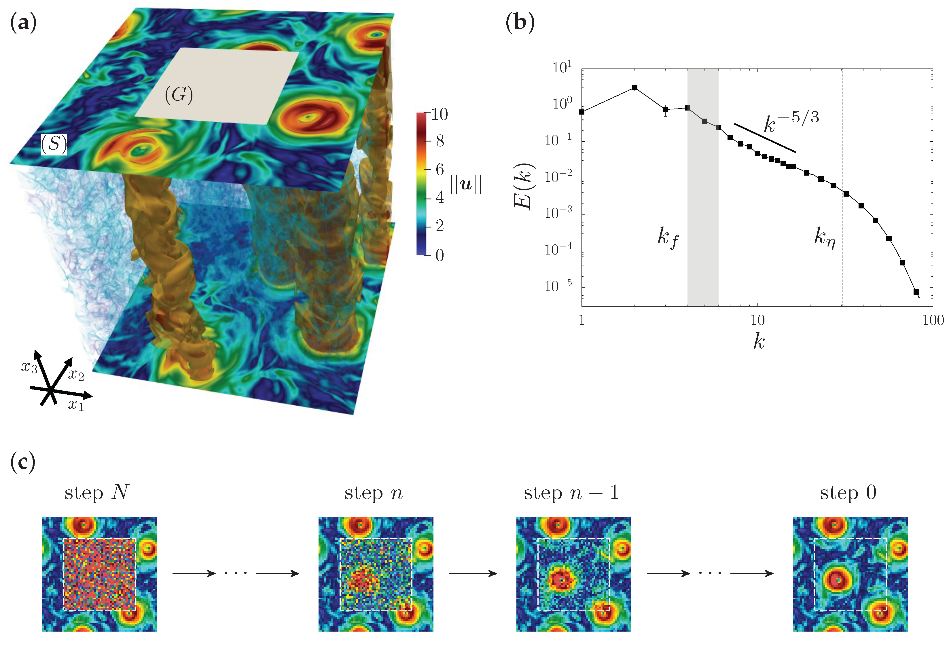
(a) Visualization of the velocity magnitude from a three-dimensional (3D) snapshot extracted from our numerical simulations. The two velocity planes (in the - directions) at the top and bottom of the integration domain show the velocity magnitude. In the 3D volume, we visualize a rendering of the small-scale velocity filaments developed by the 3D dynamics. The gray square on the top level is an example of the damaged gap area, denoted as , while the support where we assume to have the measurements is denoted as , and their union defines the full 2D image, . A velocity contour around the most intense regions () highlights the presence of the quasi-2D columnar structures (almost constant along -axis), due to the effect of the Coriolis force induced by the frame rotation. (b) Energy spectra averaged over time. The range of scales where forcing is active is indicated by the gray band. The dashed vertical line denotes the Kolmogorov dissipative wavenumber. The reconstruction of the gappy area is based on a downsized image on a grid of collocation points, which corresponds to a resolution of the order of . (c) Sketch illustration of the reconstruction protocol of a diffusion model (DM) in the backward phase (see later), which uses a Markov chain to progressively generate information through a neural network.
Figure 1.
(a) Visualization of the velocity magnitude from a three-dimensional (3D) snapshot extracted from our numerical simulations. The two velocity planes (in the - directions) at the top and bottom of the integration domain show the velocity magnitude. In the 3D volume, we visualize a rendering of the small-scale velocity filaments developed by the 3D dynamics. The gray square on the top level is an example of the damaged gap area, denoted as , while the support where we assume to have the measurements is denoted as , and their union defines the full 2D image, . A velocity contour around the most intense regions () highlights the presence of the quasi-2D columnar structures (almost constant along -axis), due to the effect of the Coriolis force induced by the frame rotation. (b) Energy spectra averaged over time. The range of scales where forcing is active is indicated by the gray band. The dashed vertical line denotes the Kolmogorov dissipative wavenumber. The reconstruction of the gappy area is based on a downsized image on a grid of collocation points, which corresponds to a resolution of the order of . (c) Sketch illustration of the reconstruction protocol of a diffusion model (DM) in the backward phase (see later), which uses a Markov chain to progressively generate information through a neural network.

Figure 2.
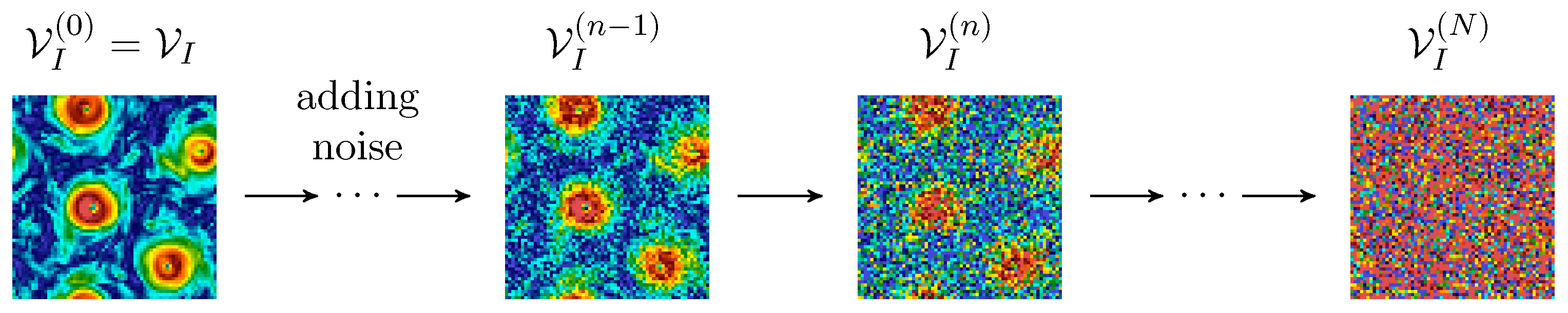
Diagram of the forward process in the DM framework. Starting with the original field , Gaussian noise is incrementally added over N diffusion steps, transforming the original image into white noise on the same resolution grid, .
Figure 2.
Diagram of the forward process in the DM framework. Starting with the original field , Gaussian noise is incrementally added over N diffusion steps, transforming the original image into white noise on the same resolution grid, .

Figure 3.
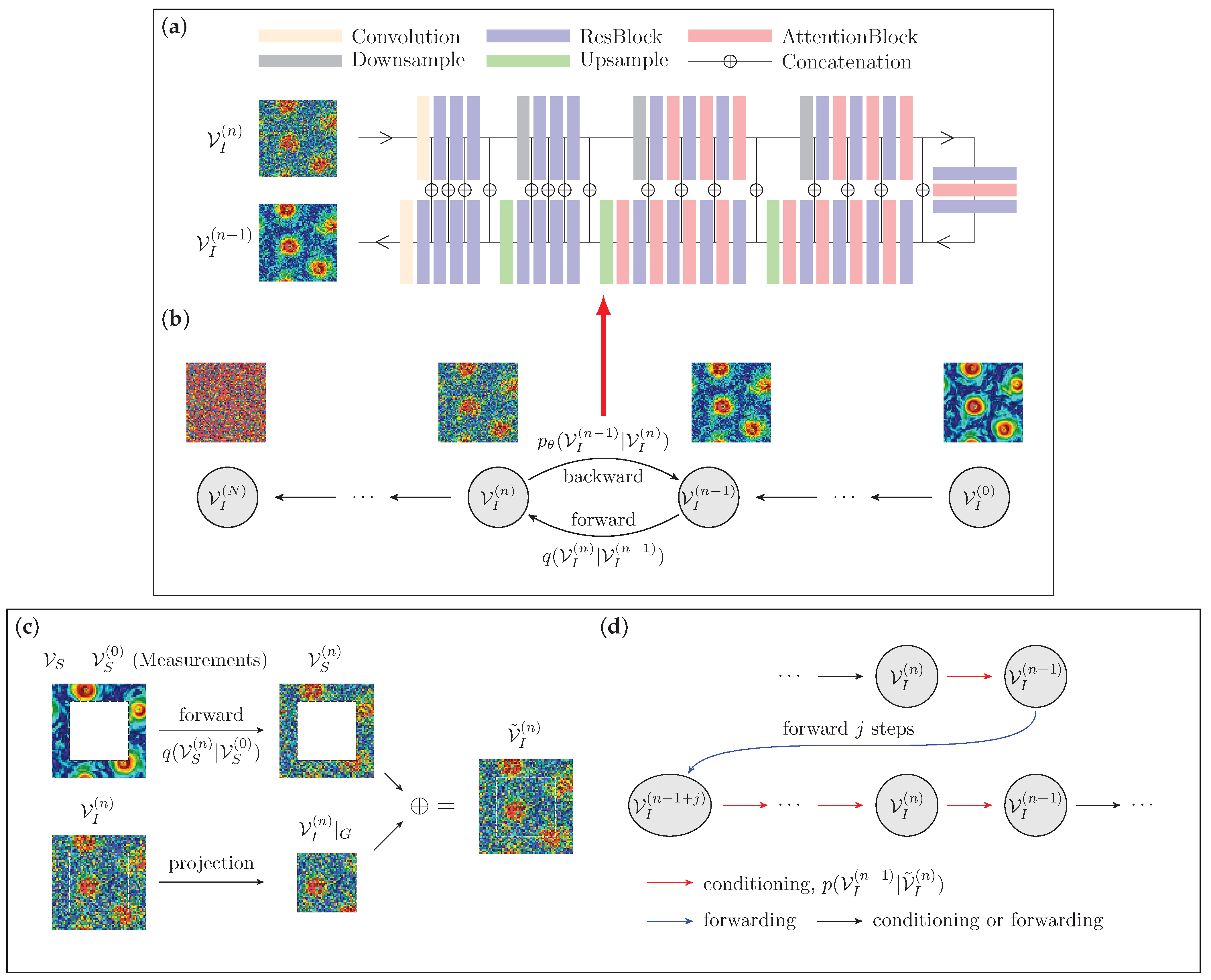
Schematic representation of the DM flow field generation framework used by RePaint for flow reconstruction. (a,b) Training stage: (a) the neural network architecture, U-Net [62], that takes a noisy flow field as input at step n and predicts a denoised field at step ; (b) The scheme of the forward and backward diffusion Markov processes. The forward process (from right to left) incrementally adds noise over N steps, while the backward process (from left to right), modeled by the U-Net, iteratively reconstructs the flow field by denoising the noisy data. More details on the network architecture can be found in Appendix B. (c,d) Reconstruction stage starting from a damaged field with a square mask. (c) Conditioning the backward process with the measurement, , involves projecting the noisy state of the entire 2D field, , onto the gap region, , and combining it with the noisy measurement, , obtained from the forward process up to the corresponding step. In this way, we obtain and then enforce the conditioning by inputting it into a backward step. (d) A resampling approach is used to deal with the incoherence in introduced by the ‘rigid’ concatenation. First, we perform a backward step to obtain , and then some noise is added by j forward steps (blue arrow). Finally, the field is resampled backwards by the same number of iterations, going back to the original step.
Figure 3.
Schematic representation of the DM flow field generation framework used by RePaint for flow reconstruction. (a,b) Training stage: (a) the neural network architecture, U-Net [62], that takes a noisy flow field as input at step n and predicts a denoised field at step ; (b) The scheme of the forward and backward diffusion Markov processes. The forward process (from right to left) incrementally adds noise over N steps, while the backward process (from left to right), modeled by the U-Net, iteratively reconstructs the flow field by denoising the noisy data. More details on the network architecture can be found in Appendix B. (c,d) Reconstruction stage starting from a damaged field with a square mask. (c) Conditioning the backward process with the measurement, , involves projecting the noisy state of the entire 2D field, , onto the gap region, , and combining it with the noisy measurement, , obtained from the forward process up to the corresponding step. In this way, we obtain and then enforce the conditioning by inputting it into a backward step. (d) A resampling approach is used to deal with the incoherence in introduced by the ‘rigid’ concatenation. First, we perform a backward step to obtain , and then some noise is added by j forward steps (blue arrow). Finally, the field is resampled backwards by the same number of iterations, going back to the original step.

Figure 4.
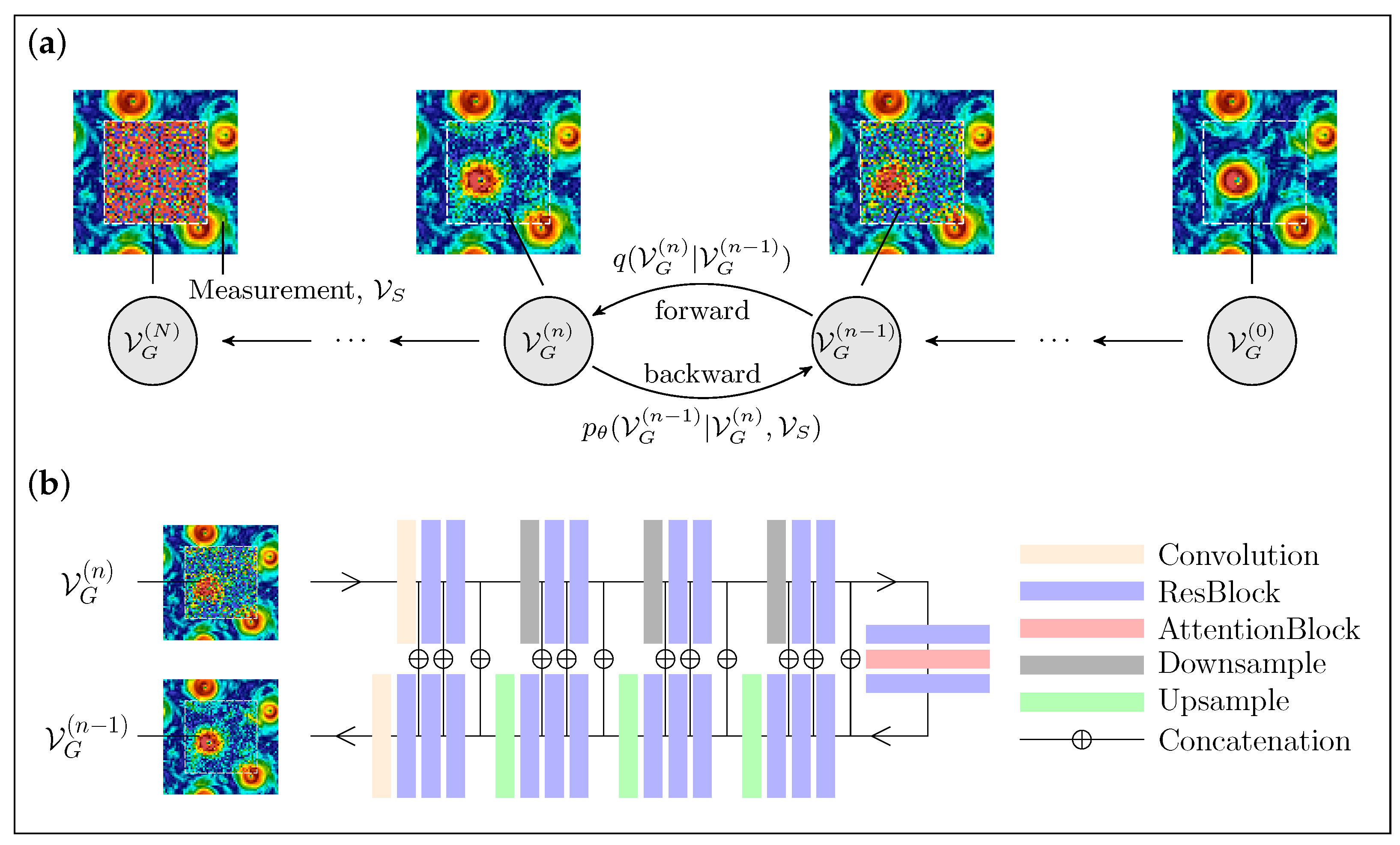
Schematic of the DM Palette protocol. (a) In the backward process (from left to right), we start from pure noise in the gap, , combined with the measurements in the frame, , to progressively denoise the missing information using the U-Net architecture described in (b). (b) A sketch of the U-Net integrating the measurement, , and the noisy data within the gap, , for a backward step.
Figure 4.
Schematic of the DM Palette protocol. (a) In the backward process (from left to right), we start from pure noise in the gap, , combined with the measurements in the frame, , to progressively denoise the missing information using the U-Net architecture described in (b). (b) A sketch of the U-Net integrating the measurement, , and the noisy data within the gap, , for a backward step.

Figure 5.
(a) The mean squared error (MSE) between the true and the generated velocity magnitude, as obtained from GAN, RePaint, and Palette, for a square gap with variable size. Error bars indicate the standard deviation. The red horizontal line represents the uncorrelated baseline MSE, . (b) The Jensen–Shannon (JS) divergence between the probability density functions (PDFs) for the true and generated velocity magnitude. The mean and error bars represent the average and range of variation of the JS divergence across 10 batches, each with 2048 samples.

Figure 6.
PDFs of the velocity magnitude in the missing region obtained from (a) GAN, (b) RePaint, and (c) Palette for a square gap of variable size (triangle), (cross), and (diamond). The PDF of the true data over the whole region is plotted for reference (solid black line) and is the standard deviation of the original data over the full domain.

Figure 7.
The PDFs of the spatially averaged error for a single flow configuration obtained from GAN, RePaint, and Palette models. The gap size changes from (a) , to (b) and (c) .
Figure 7.
The PDFs of the spatially averaged error for a single flow configuration obtained from GAN, RePaint, and Palette models. The gap size changes from (a) , to (b) and (c) .

Figure 8.
Examples of reconstruction of an instantaneous field (velocity magnitude) for a square gap of size (a) , (b) and (c) . The damaged fields are shown in the first column, while the second to fourth columns, circled by a red rectangle, show the reconstructed fields obtained from GAN, RePaint, and Palette. The ground truth is shown in the fifth column.

Figure 9.
(a) MSE and (b) JS divergence between the PDFs for the gradient of the original and generated velocity magnitude, as obtained from GAN, RePaint, and Palette, for a square gap with variable size. The red horizontal line in (a) represents the uncorrelated baseline, equal to 2. Error bars are obtained in the same way as in Figure 5.

Figure 10.
The PDFs of the gradient of the reconstructed velocity magnitude in the missing region obtained from (a) GAN, (b) RePaint, and (c) Palette, for a square gap of variable size (triangle), (cross), and (diamond). The PDF of the true data over the whole region is plotted for reference (solid black line) and is the standard deviation of the original data over the full domain.

Figure 11.
The gradient of the velocity magnitude fields shown in Figure 8. The first column shows the damaged fields with a square gap of size (a) , (b) and (c) . Note that for the case , the gap extends almost to the borders, leaving only a single vertical velocity line on both the left and right sides, where the original gradient field is missing. The gradient of the reconstructions from GAN, RePaint, and Palette, shown in the second to fourth columns, is surrounded by a red rectangle for emphasis, while the fifth column shows the ground truth.

Figure 12.
Energy spectra of the original velocity magnitude (solid black line) and the reconstructions obtained from (a) GAN, (b) RePaint, and (c) Palette for a square gap of sizes (triangle), (cross), and (diamond). The corresponding is shown in (d–f), where and are the spectra of the reconstructed fields and the ground truth, respectively.

Figure 13.
The flatness of the original field (solid black line) and the reconstructions obtained from (a) GAN, (b) RePaint, and (c) Palette for a square gap of sizes (triangle), (cross), and (diamond).
Figure 13.
The flatness of the original field (solid black line) and the reconstructions obtained from (a) GAN, (b) RePaint, and (c) Palette for a square gap of sizes (triangle), (cross), and (diamond).

Figure 14.
Probabilistic reconstructions from DMs for a fixed measurement outside a square gap with size for a configuration where all models give quite small reconstruction errors. (a) PDFs of the spatially averaged error over different reconstructions obtained from RePaint and Palette. The blue vertical dashed line indicates the error for the GAN case. (b) The damaged measurement and ground truth, inside a red box, and the prediction from GAN. (c) The reconstructions from RePaint with a small error (S), the mean error (M), and with a large error (L). (d) The reconstructions from Palette corresponding to a small error (S), the mean error (M), and a large error (L).

Figure 15.
Similar to Figure 14, but for a flow configuration chosen for its large reconstruction errors from GAN, RePaint, and Palette. The red box contains the damaged measurement and ground truth.
Figure 15.
Similar to Figure 14, but for a flow configuration chosen for its large reconstruction errors from GAN, RePaint, and Palette. The red box contains the damaged measurement and ground truth.

Disclaimer/Publisher’s Note: The statements, opinions and data contained in all publications are solely those of the individual author(s) and contributor(s) and not of MDPI and/or the editor(s). MDPI and/or the editor(s) disclaim responsibility for any injury to people or property resulting from any ideas, methods, instructions or products referred to in the content. |
© 2023 by the authors. Licensee MDPI, Basel, Switzerland. This article is an open access article distributed under the terms and conditions of the Creative Commons Attribution (CC BY) license (https://creativecommons.org/licenses/by/4.0/).
Share and Cite
MDPI and ACS Style
Li, T.; Lanotte, A.S.; Buzzicotti, M.; Bonaccorso, F.; Biferale, L. Multi-Scale Reconstruction of Turbulent Rotating Flows with Generative Diffusion Models. Atmosphere 2024, 15, 60. https://doi.org/10.3390/atmos15010060
AMA Style
Li T, Lanotte AS, Buzzicotti M, Bonaccorso F, Biferale L. Multi-Scale Reconstruction of Turbulent Rotating Flows with Generative Diffusion Models. Atmosphere. 2024; 15(1):60. https://doi.org/10.3390/atmos15010060
Chicago/Turabian StyleLi, Tianyi, Alessandra S. Lanotte, Michele Buzzicotti, Fabio Bonaccorso, and Luca Biferale. 2024. "Multi-Scale Reconstruction of Turbulent Rotating Flows with Generative Diffusion Models" Atmosphere 15, no. 1: 60. https://doi.org/10.3390/atmos15010060
Note that from the first issue of 2016, this journal uses article numbers instead of page numbers. See further details here.