Gap-Filling and Missing Information Recovery for Time Series of MODIS Data Using Deep Learning-Based Methods


1
School of Geography and Planning, Sun Yat-sen University, Guangzhou 510275, China
2
School of Atmospheric Sciences, Sun Yat-sen University, Zhuhai 519082, China
3
Beidou Research Institute, Faculty of Engineering, South China Normal University, Foshan 528000, China
*
Author to whom correspondence should be addressed.
Remote Sens. 2022, 14(19), 4692; https://doi.org/10.3390/rs14194692
Submission received: 16 August 2022
/
Revised: 11 September 2022
/
Accepted: 15 September 2022
/
Published: 20 September 2022
Abstract
:Sensors onboard satellite platforms with short revisiting periods acquire frequent earth observation data. One limitation to the utility of satellite-based data is missing information in the time series of images due to cloud contamination and sensor malfunction. Most studies on gap-filling and cloud removal process individual images, and existing multi-temporal image restoration methods still have problems in dealing with images that have large areas with frequent cloud contamination. Considering these issues, we proposed a deep learning-based method named content-sequence-texture generation (CSTG) network to generate gap-filled time series of images. The method uses deep neural networks to restore remote sensing images with missing information by accounting for image contents, textures and temporal sequences. We designed a content generation network to preliminarily fill in the missing parts and a sequence-texture generation network to optimize the gap-filling outputs. We used time series of Moderate-resolution Imaging Spectroradiometer (MODIS) data in different regions, which include various surface characteristics in North America, Europe and Asia to train and test the proposed model. Compared to the reference images, the CSTG achieved structural similarity (SSIM) of 0.953 and mean absolute errors (MAE) of 0.016 on average for the restored time series of images in artificial experiments. The developed method could restore time series of images with detailed texture and generally performed better than the other comparative methods, especially with large or overlapped missing areas in time series. Our study provides an available method to gap-fill time series of remote sensing images and highlights the power of the deep learning methods in reconstructing remote sensing images.
1. Introduction
The rapid development of remote sensing technology provides abundant earth observation images at varied spectral, spatial, and temporal resolutions and promotes a broad range of applications, such as land cover and land use classification [1,2], map vectorization [3], land surface phenology monitoring [4,5], and natural disaster modeling [6,7]. Multispectral imaging sensors that typically operate in a few spectral bands ranging from visible, near infrared, and shortwave infrared wavelengths are common among a variety of remote sensing sensors, as the multispectral imaging system acquires the images of the earth’s surface by detecting solar radiation reflected from targets on the ground. The utility of multispectral images is limited by large amounts of missing information in the remote sensing data due to cloud contamination and sensor malfunction [8]. Restoring missing information and gap-filling for remote sensing images help provide continuous and consistent data for downstream applications.
A number of methods for image gap-filling have been developed in studies. One approach is to apply image inpainting techniques to individual remote sensing images with gaps. Studies have developed image inpainting techniques, such as homomorphic filtering [9], linear histogram matching [10], and other transformation methods, to enhance the weak information in the images due to cloud contamination. These methods are useful to recover land surface information influenced by thin clouds, but they encounter difficulties in areas covered by thick clouds and often generate blurred images. There are also image inpainting techniques that aim to recover missing pixels in the images by accounting for contextual information [11], such as similar pixel interpolator [12], ordinary kriging and co-kriging techniques [13,14], Markov random field model [15], and total variational method [16]. Recently, Wang et al. [17] developed an interpolation method based on space-spectral radial basis function to recover missing band information in Landsat ETM+ images. These techniques are able to reconstruct the images influenced by thick clouds in a relatively small area but often have difficulties in images with considerable missing data.
Another approach is to use supplementary information such as multi-spectral and/or multi-temporal information for image gap-filling [18]. The idea underlying the multispectral-based methods is to develop a model that reflects the relationship between contaminated band data and supplementary data from cloud-insensitive bands in multi-spectral images or from cloud-free images acquired at a similar time by the other sensors. For example, the cirrus band in Landsat 8 has been widely used to remove noise, such as haze and clouds [19,20]. Zhang et al. [21] developed the algorithm of haze optimized transformation to account for different band sensitivities to clouds and then removed cloud noise using a virtual cloud point method. Gladkova et al. [22] combined the histogram matching method and the local least square method to reconstruct the missing band 6 data from the band 7 data in MODIS-Aqua images. In recent years, the approaches of multi-sensor data fusion have been developed for image recovery [23,24]. Remote sensing images from sensors such as MODIS, Landsat 8, and Sentinel have been used in data fusion to fill the missing data in Landsat ETM+ images. Roy et al. [25] proposed a semi-physical fusion method that combined MODIS and Landsat images to remove the effects of cloud contamination from the Landsat ETM+ images. Moreno-Martínez et al. [26] developed a time-adaptive reflection fusion model by using a bias-corrected Kalman filter method to fuse Landsat with MODIS data. By comparison, the multi-temporal-based methods utilize images acquired by the same sensor but at different times as supplementary information to restore images with gaps or cloud [27]. There are a variety of techniques to replace cloudy pixels in images with cloud-free pixels from multi-temporal images [28]. The algorithm of neighborhood similar pixel interpolator [29] used images acquired at similar dates to search for pixels with similar reflectance and make predictions of the missing data. The multi-temporal weighted linear regression model [30] combined multi-temporal reference information and the non-reference regularization algorithms to predict missing values in Landsat ETM+ images. Although both multispectral-based and multi-temporal-based methods could achieve image gap-filling and remove thick clouds, both rely on supplementary images, which are often not available.
Accompanying the rapid development in computer sciences, the deep learning-based methods based on sophisticated neural networks have been developed and widely applied to reconstruct images with missing data. Goodfellow et al. [31] proposed the Generative Adversarial Nets (GAN) based on a game learning strategy for reconstructing natural images, where the generative networks randomly generate the missing parts in an image and the discriminant networks evaluate the generated results. GAN is widely used for reconstructing face pictures and landscape images [32,33]. As the models for reconstructing natural images continued to blossom, scholars used the deep learning methods to reconstruct remote sensing images. Chen et al. [34] combined multi-temporal methods with convolutional neural networks (CNN) to remove thick clouds in ZiYuan-3 satellite data. Zhang et al. [35] proposed a progressive spatiotemporal patch group learning framework that is able to recover several multi-temporal images at the same time. Li et al. [36] developed the Convolutional-Mapping-Deconvolutional Network using both optical and SAR images to realize thick cloud removal. Although the proposed framework made progress in restoring multi-temporal remote sensing images using deep learning approaches, there is room for improvements as the restored images are prone to blurring and become inaccurate when large areas have thick cloud covers or when multi-temporal images have large overlapping areas with missing data.
Aiming at addressing the above-mentioned limitations, we propose a content-sequence-texture generation (CSTG) network, which is based on a deep learning reconstruction method that accounts for restoring the content, temporal sequence, and spatial texture of images. The goal of this study is to design and evaluate the method that consists of two networks (i.e., a content generation network and a sequence-texture generation network) for recovering time series of remote sensing images with missing data. Different from most recovery methods that rely on multi-temporal information, we aim to develop a method that allows for reconstructing time series of remote sensing images simultaneously, even if there are no completely cloud-free images in the time series. The idea for the proposed deep learning network is to consider content consistency, texture details, and sequential trend information and apply both spectral loss and structure similarity loss to improve the accuracy of image reconstruction. Compared to existing methods, we aim to develop robust methods to process time series of images even with large missing areas and/or overlapped clouds on multi-temporal images.
2. Study Materials
Moderate resolution Imaging Spectroradiometer (MODIS) onboard the Terra and Aqua satellite platform provides near-daily global coverage of land surface observations. Due to cloud contamination and weather conditions, daily MODIS data have serious quality issues, and thus the MODIS science team develops and offers 8-day or 16-day composite MODIS products, which largely reduce low-quality data. There are still considerable gaps and missing data in the time series of MODIS products, making it an ideal case for gap-filling and missing information recovery studies. We used both the 500-m 8-day composite surface reflectance data of MOD09A1 and the 250-m 16-day composite vegetation index data of MOD13Q1 for studies. We used surface reflectance data in the red, blue, and near-infrared bands from both products.
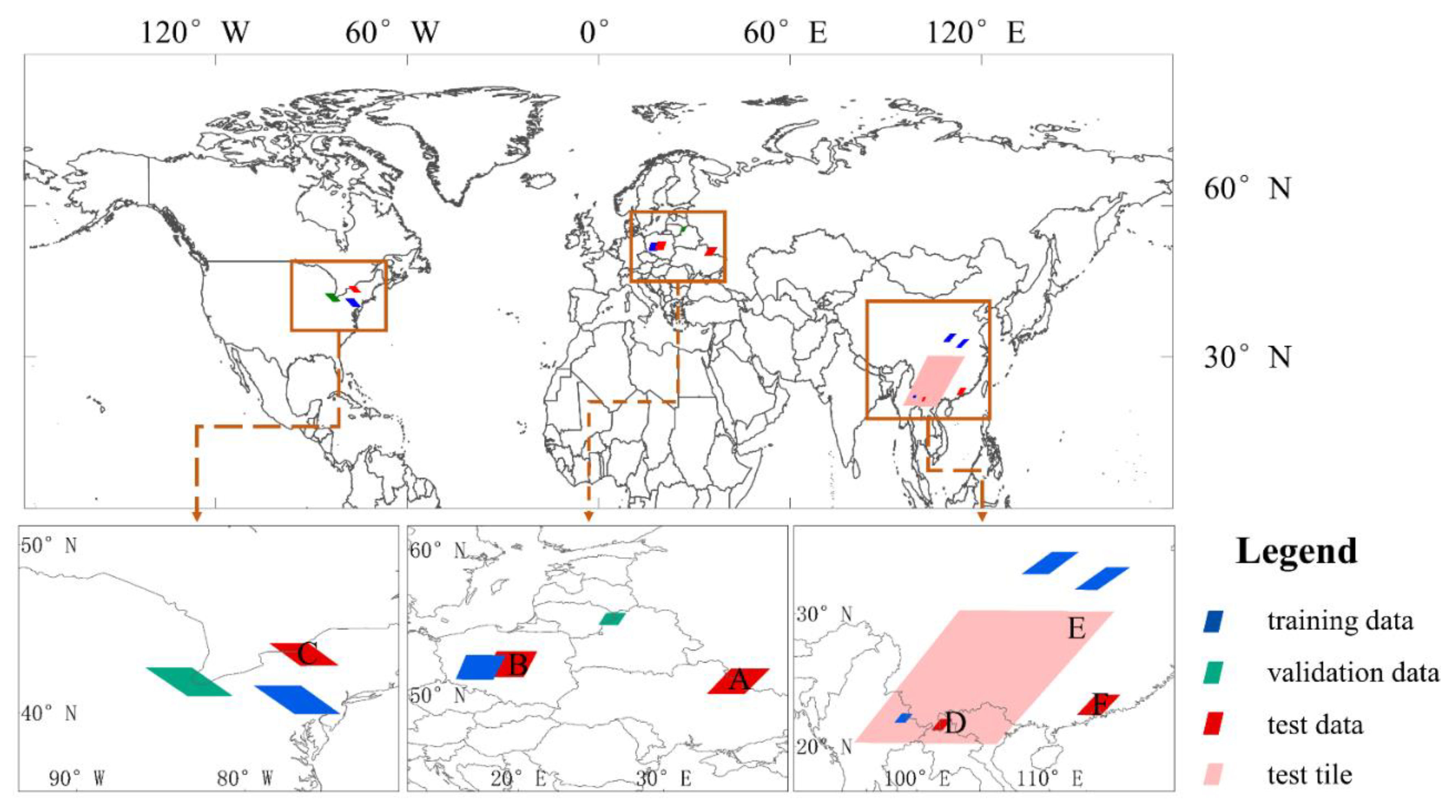
The gap-filling methods were conducted to training, validate, and test at the areas of Asia, Europe, and North America in the northern hemisphere (Figure 1). Each study dataset has an image size of 400 × 400 and the images have high-quality observations in the time series. The data with blue segments were applied to train the model and the data with green segments were used for model validation. We used the data with red segments of A–F and a whole tile image with a pink segment for model testing.
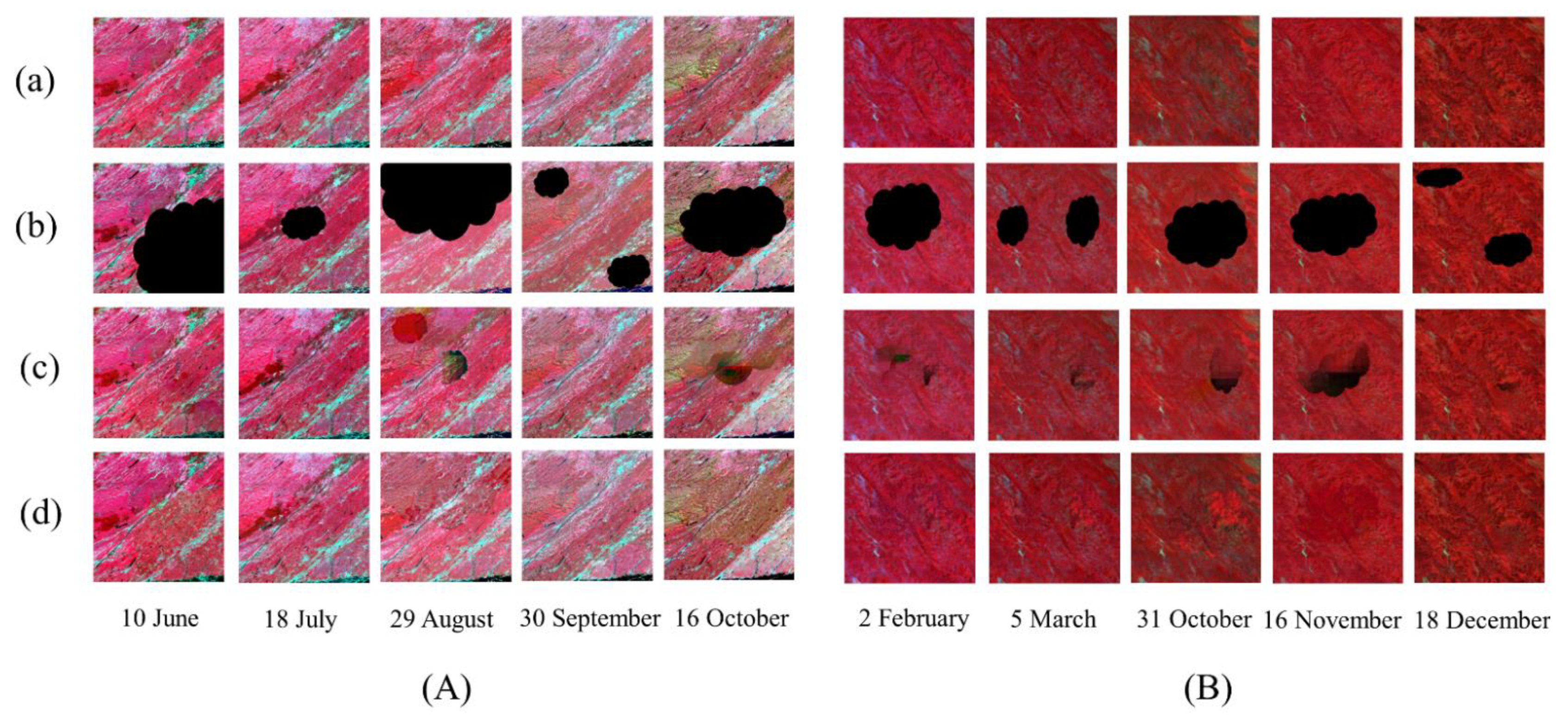
Study area A crosses the borders of Russia and Ukraine. It has a temperate continental climate with distinctive seasonal surface changes. The images used from MOD09A1 were acquired on 30 September and 8 October in 2020. Study area B is situated in the central part of Poland. The area contains several land cover types such as buildings, rivers, and vegetation. The images from MOD09A1 were acquired on 26 February and 29 August in 2019. Study area C is located along the Atlantic coast in the northeastern United States. The data from MOD09A1 were acquired on 26 February, 22 March, 23 April, and 17 November in 2016. Study area D crosses the border between China and Myanmar. Most of the study areas are located in Yunnan in China with a small area that covers the northeastern portion of Myanmar. The data from MOD13Q1 were acquired on 2 February, 5 March, 31 October, 16 November, and 18 December in 2019. Study area E comes from the entire tile (4800 × 4800) of H27V06 in MOD13Q1 acquired on 25 June in 2019. The H27V06 tile covers southwestern China, Hanoi, Laos, Thailand, and northern Myanmar. The remote sensing images in this area are prone to cloud contamination in summer due to the influence of monsoon climate. The area with cloud contamination in the study image exceeds two-third of the entire image, representing a challenging case for gap-filling. Study area F is located near the Pearl River estuary. The study images from MOD09A1 were acquired on 18 February, 21 March, 22 April, 15 October, and 24 November in 2020. There are lush vegetation and a wide variety of species in the study area with a subtropical monsoon climate. The climate is hot and humid, making it suitable for testing the ability of the models. All the products we used in this research are listed in Table 1.
We divided the test data into two categories (artificial dataset and observed dataset) to assess the performance of the developed network. The artificial dataset is the cloud data derived from original cloud-free images preprocessed by artificial masks and is used to compare the reconstruction results with the original images quantitatively to assess the model’s accuracy. The observed dataset is original images contaminated by clouds, for demonstrating the practical ability of the model. Each category was applied to two time steps: individual image and time series of images at regional or large-scale missing area, respectively.
3. Methodology
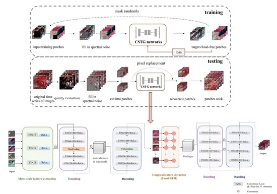
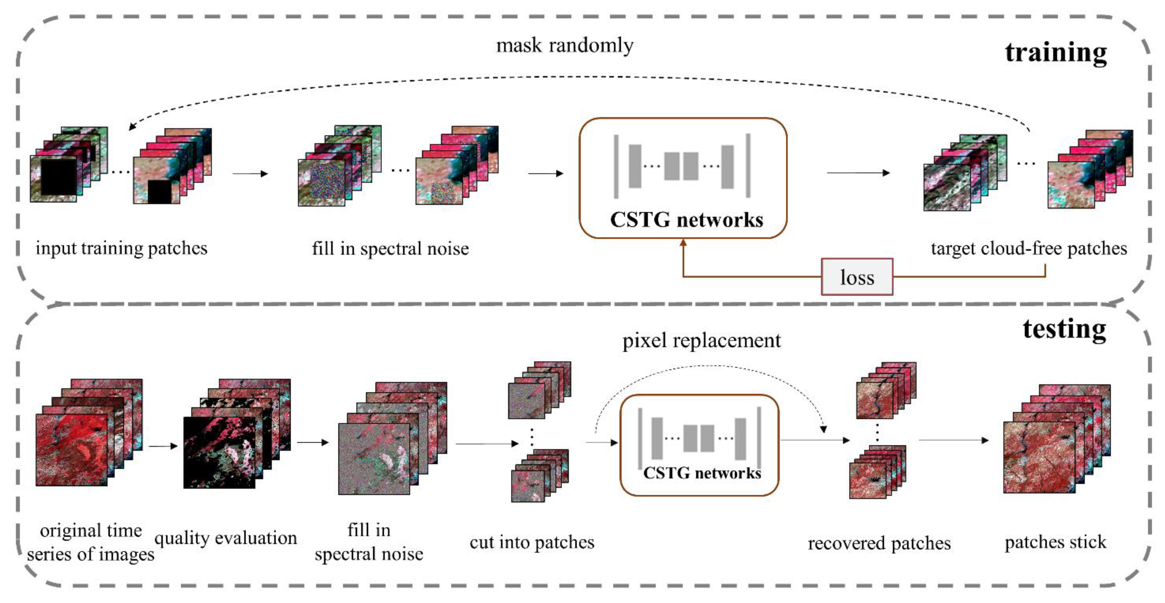
To address the limitations associated with methods in previous research, we proposed a gap-filling and image recovery method for a time series of images based on a network of content-sequence-texture generation. The overall flowchart of the proposed method is shown in Figure 2. In the training process, we chose several cloud-free images with time series information and cut them into patches, which were considered as target data. We added masks with random positions and sizes into the cloud-free patches and filled in the mask areas with random spectral noise as the network input. When conducting model testing, we stacked the time series images for restoration and excluded pixels with clouds and/or poor qualities in the images based on quality control data. Time series images were then split into smaller patches. The image patches were put into a content generation network to fill gaps initially and obtain general content. And a sequence-texture generation network was used to refine the texture details in order to reduce the texture and spectral differences. After mosaicking gap-filled patches into the generated maps, the corresponding pixels in the generated maps were selected to replace the mask areas in the original images. The high-quality, gap-filled images are generated as follows:
where denotes the final high-quality result, denotes feature maps generated by CSTG network and represents the original image after poor-pixel masking. denotes the corresponding quality map of . In the quality map , zero represents poor quality and one represents high quality. denotes the point multiplication operation between two matrices.
3.1. Data Quality Evaluation and Preprocessing
To fill gaps in remote sensing images, it is necessary to determine the pixels and areas that are contaminated by clouds or have low quality. There are various methods for detecting low-quality data in the products derived from different sensors. For instance, FMask [37] and MSCFF [38] algorithms have been used to extract the masks of clouds from Landsat and Sentinel data, respectively. The MODIS products provide a layer of state flags, which consists of binary codes to represent the quality of observations for each pixel. Although the quality control data in the MODIS products are helpful to extract pixels with poor qualities, there are often cloudy pixels that are missed in the quality control data. As the reflectance of clouds in visible bands is much higher than that of other objects, we conservatively masked out the pixels with reflectance more than 0.25 in the visible bands. To reduce speckle noise, we expanded the masks using the method of 5-pixel morphological dilation. Then we filled in masked areas with random noise, which follows normal distribution with the same mean value and variance as high-quality surrounding areas. The random noise helps enhance spectral information in the original image and can be written as:
where denotes a set of random variables for filling in masked areas; and are the mean value and the variance of the normal distribution, respectively, and can be calculated as:
where denotes the surface reflectance of the pixel located at the coordinates ; and denote the weight and the height of the image, respectively; denotes the aggregation of all masked pixels, and denotes the total number of masked pixels.
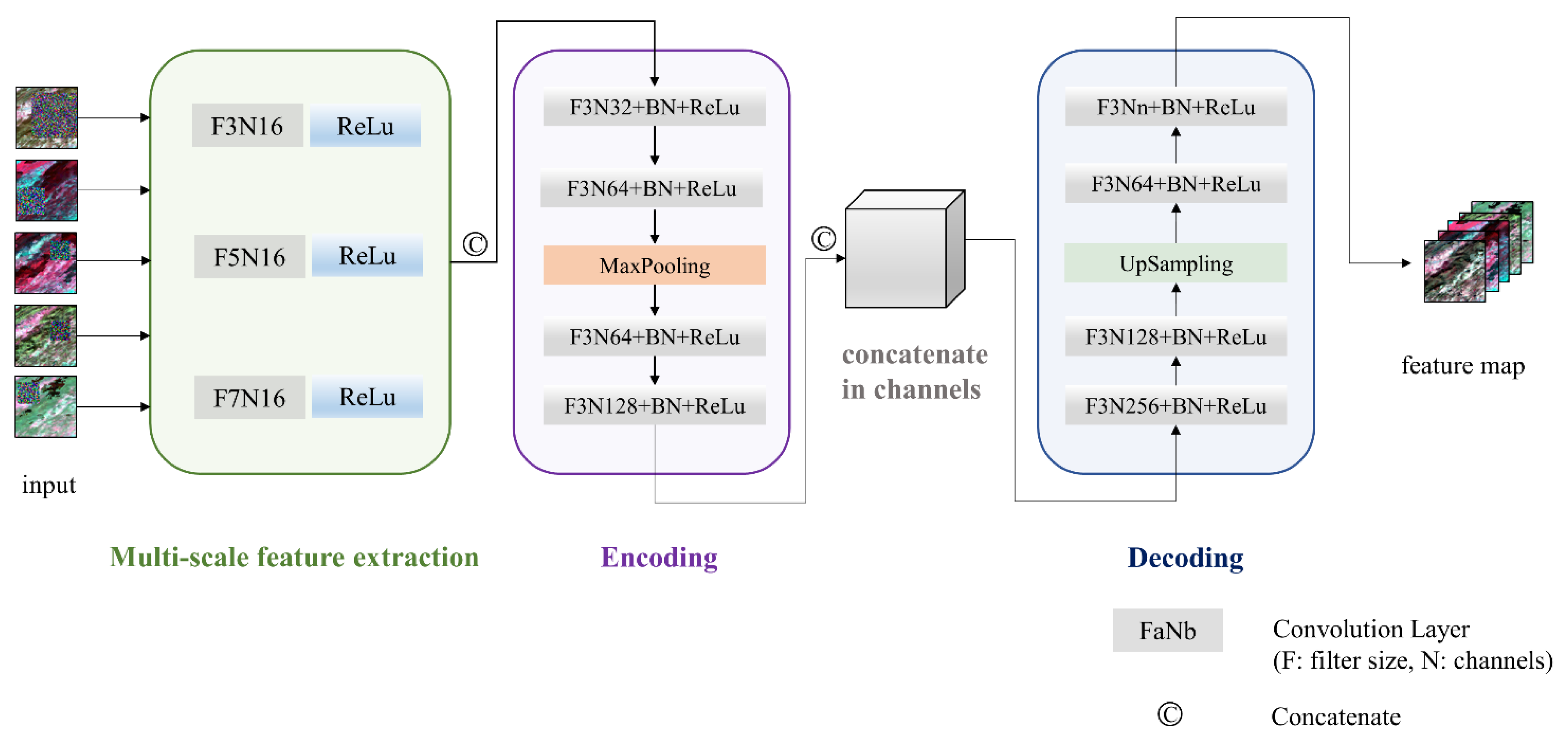
3.2. The Content Generation Network
The content generation network as shown in Figure 3 is used to initially fill the gaps in the images based on supplementary information from the other images in the time series. It consists of three components: multi-scale feature extraction module, feature encoding module, and decoding module. Typically, the convolution kernel sizes are small. Odd integer values make them convenient for use as a padding strategy and make it easy to locate the output pixels. We set the kernel sizes of three, five and seven, respectively, to perform the multi-scale feature extraction for each image in the time series. After concatenating extracted features, a network structure that is similar to the auto-encoder was constructed to fill in the missing area of the images. We encoded multi-scale features using a MaxPooling layer to compress the input size and increase the receptive field while retaining as many detailed features as possible. Several convolution blocks, of which each was composed of a convolution layer, a batch normalization layer (BN), and a rectified linear unit (ReLU), were designed to extract features. Then we concatenated features from each time step in the channel dimension. We employed decoding with several convolution blocks and an UpSampling layer to ensure that the feature maps have the same size as the input maps. All the features were compressed into a feature group with a series of feature maps, and the number of feature maps was equal to the summary of the bands in the input time series. Studies have proved that loss functions with considerations on both global and local scales may have good performance on cloud removal [35]. The loss function of the content generation network is defined based on root mean squared errors (RMSEs) between the output feature maps and the target maps, which refer to the high-quality input data before masking randomly.
The loss function consists of both global loss and local loss as follows:
Global loss refers to RMSEs calculated for the entire image patches, and local loss refers to RMSEs calculated for the masked areas in the image patches. Global loss helps improve global consistency of the generated feature map and local loss helps improve local consistency of the recovered area. The equations for global and local losses are as follows:
where denotes the total loss of the content generation network; and denote global loss and local loss, respectively; and denote the weight and the height of an image patch, respectively; m denotes the total number of the mask pixels; denotes the set of mask pixels; denotes the predicted surface reflectance in the output feature maps of the pixel located at the coordinates and ; and denotes the observed surface reflectance in the target maps of the pixel located at the coordinates and .
3.3. The Sequence-Texture Generation Network
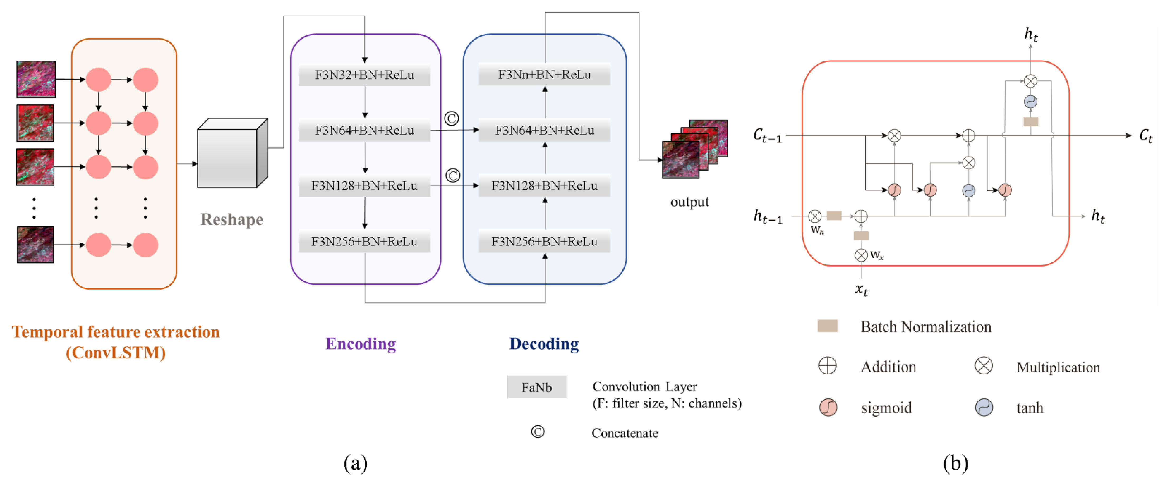
The sequence-texture generation network accounts for changes in the time series of images at the same position and the texture characteristics of neighbor pixels for missing information recovery. The core idea of the network is to learn spectral change information in the time series with recurrent neural networks (RNN) and contextual information from the neighboring cloud-free areas with convolutional neural networks (CNN) and further enrich the spatiotemporal information in the feature map obtained by content generation. LSTM-CNN is used as the model structure (Figure 4a). In the model structure, ConvLSTM [39] is used to extract time series features of the input images. LSTM is a deep learning network that is suitable for tackling sequential problems with regular time intervals [40]. ConvLSTM inherits the long-term memory functions and sequence modeling advantages of LSTM which could catch information from previous time steps. The main difference between ConvLSTM and LSTM is the dimension of the input data. The input of LSTM is one-dimension data, which makes it difficult to deal with spatial-temporal images or videos, while ConvLSTM expands the dimension of the input data into three to solve this problem. Another improvement is that ConvLSTM uses convolution operation to calculate the cell output and the hidden layer state, instead of single matrix multiplication used in LSTM. Figure 4b illustrates the internal structure of a ConvLSTM cell at a given time step. The cell runs through three self-parameterized controlling gates, i.e., input gate (), forget gate (), and output gate (), and these are calculated as follows:
The cell output and the hidden state can be calculated as:
where denotes the input at time step ; denotes the output of the past cell; denotes the past hidden states; and are the different weights and bias in the input gate, the forget gate, the output gate, and the cell output; and denote the convolution operator and the Hadamard product, respectively. In general, the unit at time step receives both cell status and outputs from the unit at the previous time step, and passes both the cell status and outputs to the unit at the next time step, thereby forming a time sequence memory.
A CNN with a residual connection structure was used for texture generation. The residual connection structure breaks the symmetry of CNN and helps pass detailed information to the decoding layers such that it improves the representation of the deep network. The networks described above are able to generate gap-filled maps with continuous spectral reflectance and detailed texture.
The loss function for the sequence-texture generation network consists of both spectrum (SPE) loss and structural similarity (SSIM) loss, which is calculated as:
where , , and denote the overall loss, spectrum loss, and structural similarity loss, respectively. is a balanced parameter that is empirically set to 0.01. The SPE loss is defined based on RMSE as the sum of global loss and local loss:
SSIM accounts for the similarity of brightness, contrast, and structure of two images, whereas the loss function is defined as follows:
where and denote the mean values of the output feature maps and the target maps, respectively; , , and denote the variance of the output, the variance of the target, and their covariance, respectively; and and denote two different equilibrium parameters.
4. Experiment Design
4.1. Model Training and Setup
We normalized each group of training datasets and cut them into small patches with a window size of 32 × 32. The cropping stride was set to 20, such that the patches overlapped. The generated patches were augmented in five directions, i.e., the patches were rotated 90°, 180°, and 270°, respectively and flipped both vertically and horizontally. We obtained 24,000 groups of training patches and 4800 validation patches for the content generation network training. Holdout validation was used to evaluate the model performance during the training process. Different from cross validation, hold out procedure means the training set and the validation set are independent and have no intersection with each other. In our study, we chose seven different study areas, five for making a training set and two for a validation set. In each epoch, we added masks with random positions and sizes to multi-temporal patches and filled with spectral noise. When we finished each training epoch and obtained the model, the validation data is fed into the model to evaluate the model performance on the data set that is completely different from the training data.
We generated 20 sets of cloud masks with random positions and radiuses and added the masks to sequential patches. After filling gaps using the content generation network, we obtained 20 sets of data for sequence-texture generation, of which 16 were used as the training datasets, and the remaining four were used as the validation sets. We cut the training datasets into 32 × 32 patches and augmented the data by rotating and flipping. Finally, 38,400 groups of training patches and 9600 groups of validation patches were generated for the sequence-texture generation network.
The networks were implemented based on the Tensorflow framework using the Adam [41] adaptive optimization method for training, which were conducted on the Ubuntu 18.04.2 system (published by Canonical in 26 April 2018 in London, England) equipped with NVIDIA RTX 2080Ti GPUs. The initial learning rate for the content generation network and the sequence-texture generation network were set as 0.0005 and 0.001, respectively, and the attenuation coefficients were both set as 0.8 at the intervals of 500 epochs. We trained each network with 1000 epochs and eventually selected the model with the lowest validation loss as the final model for testing.
4.2. Model Comparisons
We also introduced several existing methods designed for other remote sensing products to compare the results, including weighted linear regression (WLR) proposed by Zeng et al. [30], spatial-temporal-spectral (STS) joint CNN developed by Zhang et al. [42], Chen’s method [34], and Zhang’s method [35]. Among these methods, WLR is designed for Landsat ETM+ SLC-off imagery; STS and Zhang’s method are generally applied in Landsat and Sentinel-2 data; and Chen’s method is for ZY-3 image reconstruction. All of them were applied in this research to restore artificial missing areas and conduct gap-filling for individual images.
The WLR used a linear relationship to derive missing values from locally similar pixels. It selected similar pixels according to a searching window and accounted for both spatial and spectral differences to calculate the weights of each similar pixel. The WLR also used a regularization method to deal with the situation when available reference images were not sufficient. The method has been packaged into executable software (http://sendimage.whu.edu.cn/send-resource-download/ (accessed on 3 November 2016)) and has proven its performance on artificial and observed Landsat SLC-off ETM+ images.
The STS combines spatial-temporal-spectral joint information to construct a deep CNN and applies multi-scale feature extraction units to obtain context information. Dilated convolutional layers were used to enlarge the receptive field, and skip connections were used to transfer the information from the previous layer. Studies have found the method could perform well on reconstructing both SLC-off ETM+ and Terra MODIS band 6 data.
The method developed by Chen et al. used one CNN to detect and mask cloudy areas and another CNN to fill gaps based on content, texture, and spectral generation. The idea was successfully used to recover ZY-3 multispectral and panchromatic images.
Zhang et al. took four steps to recover missing information in images, including multi-temporal cloud detection, patch group stacking and sorting, deep learning recovering model, and weighted aggregation and progressive iteration. The method developed by Zhang et al. that combines both deep learning models and mathematical models performed well on reconstructing the Landsat-8 and Sentinel-2 data.
As among above-mentioned methods, the WLR method focuses on recovering images on the basis of statistics, and the other three comparison methods are mainly based on deep learning. We retrained and predicted reconstruction results from three deep-learning-based models using the MODIS data. As WLR, STS and Chen’s method are designed for individual image reconstruction, we chose a high-quality image as a reference to recover cloudy images. As only Zhang’s method and the CSTG method can reconstruct multi-temporal images simultaneously, we further compared them in reconstruction time series of images.
4.3. Evaluation Metrics
To evaluate the method’s performance, we compared the surface reflectance in both visible and near-infrared bands. Three evaluation metrics were used, i.e., the coefficient of determination (), mean absolute error (), and structural similarity index method (). MAE is one of the most evaluative indexes that can explain the difference between model simulation and ground truth value. SSIM is widely used to measure the similarity between two images and can be regarded as an index to measure the quality of distorted images. The metrics mentioned above are calculated as follows:
where and denote the weight and the height of the image patch for testing, respectively; denotes the set of mask pixels and denotes the total number of the mask pixels; and denote predicted and observed surface reflectance for pixels located at the coordinates and , respectively; and denote the mean values of the predicted data and the observed data, respectively; , , and denote the variance of prediction, the variance of observation, and their covariance, respectively; and are equilibrium parameters.
5. Results
5.1. Experiments Based on Artificial Datasets
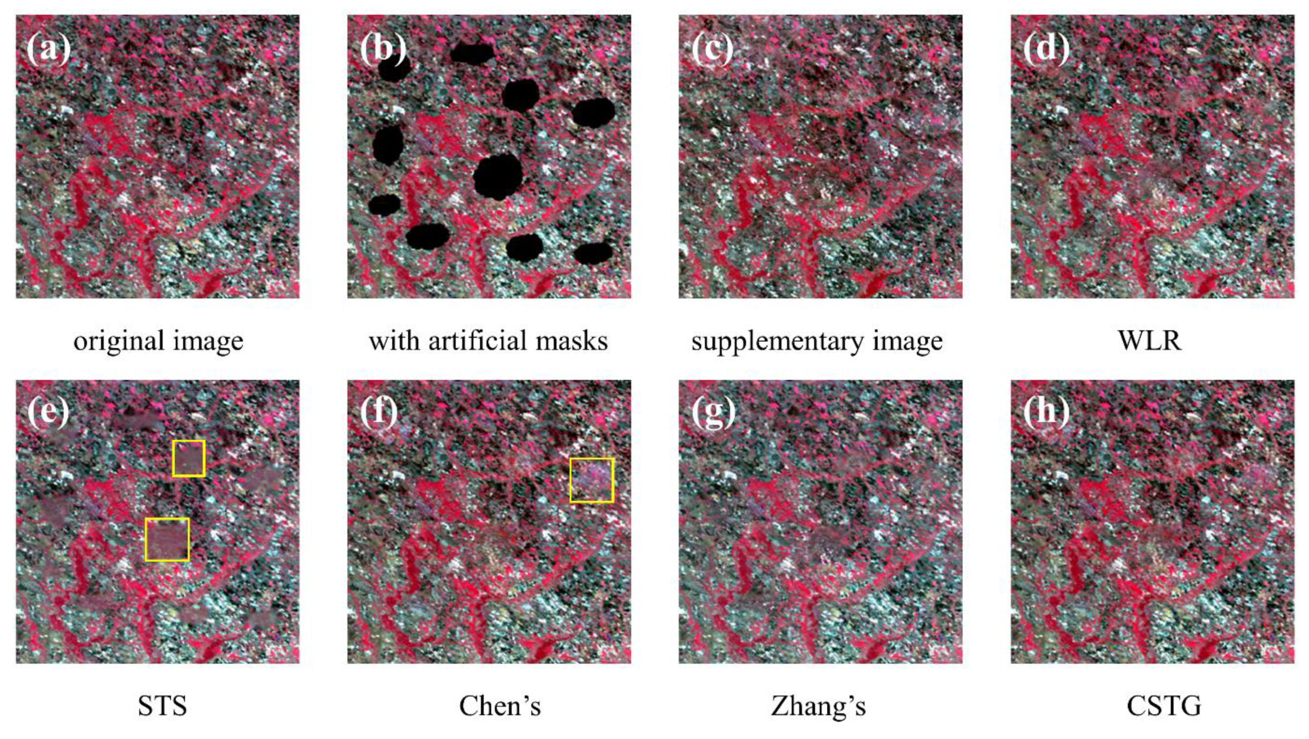
Figure 5 presents the recovery results of individual images using five different methods when applying local and dispersive masks. Visually, the images recovered based on WLR, Zhang’s method and our proposed CSTG method captured spectral and spatial characteristics of the original image well (Figure 5d,g,h). There are no obvious boundaries between the masked areas and their surroundings in the recovered images, and their results are closer to the original image than the results derived from the other methods. STS has the problem of texture blurring (e.g., the areas marked using yellow boxes in Figure 5e) and Chen’s method suffers from the problem of spectrum inconsistency (e.g., the areas marked by the yellow box in Figure 5f).
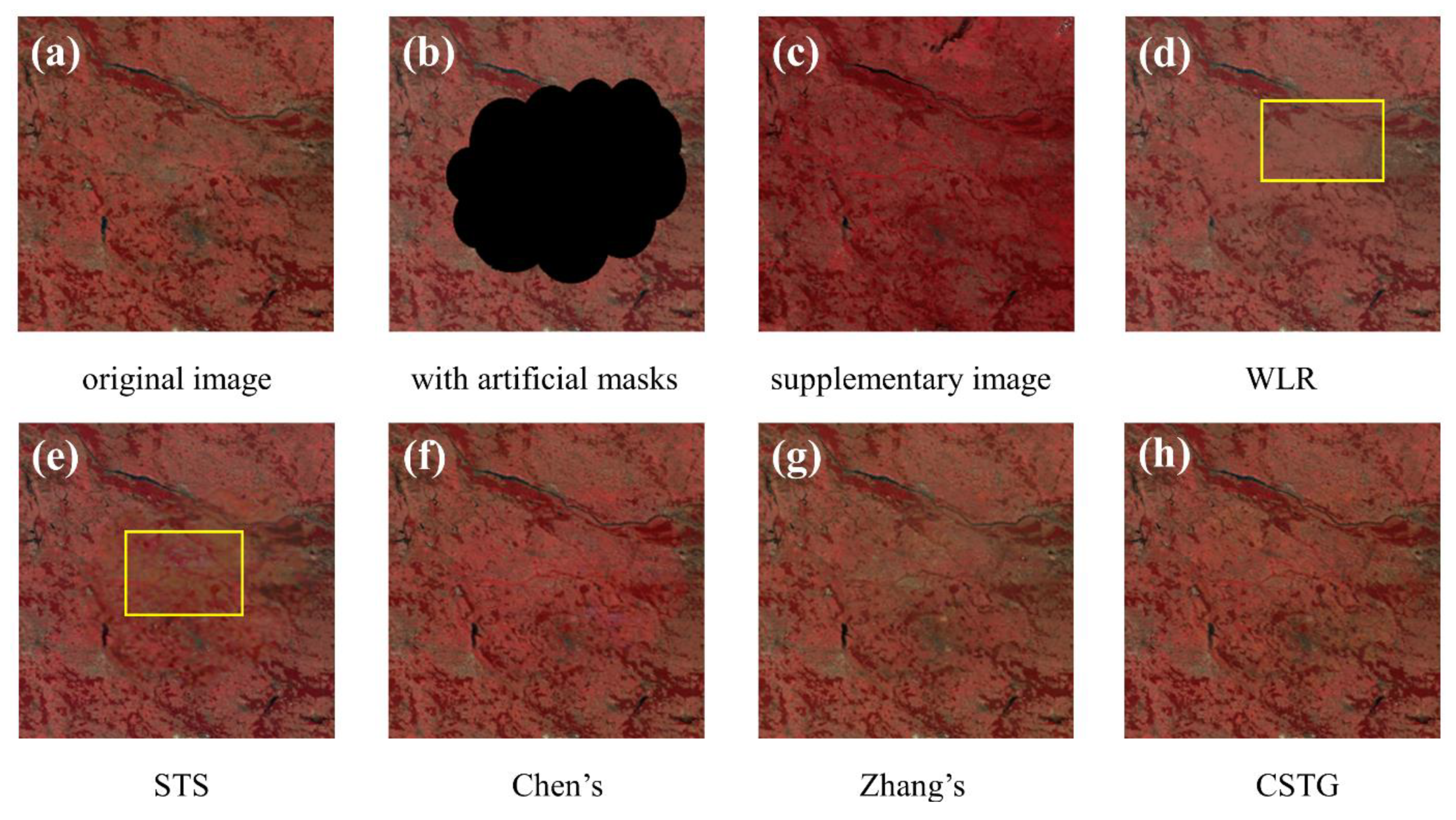
Figure 6 exhibits the recovery results of individual temporal images using five different methods when applying a large and intensive mask. The images recovered by Zhang’s method and CSTG (Figure 6g,h) are more consistent with original images than other methods. Although WLR performs well at a small scale, it has the problems of over-smoothing and missing texture details at a large scale (e.g., the yellow box in Figure 6d). Both STS and Chen’s method appear to have the same problems as those in Figure 5.
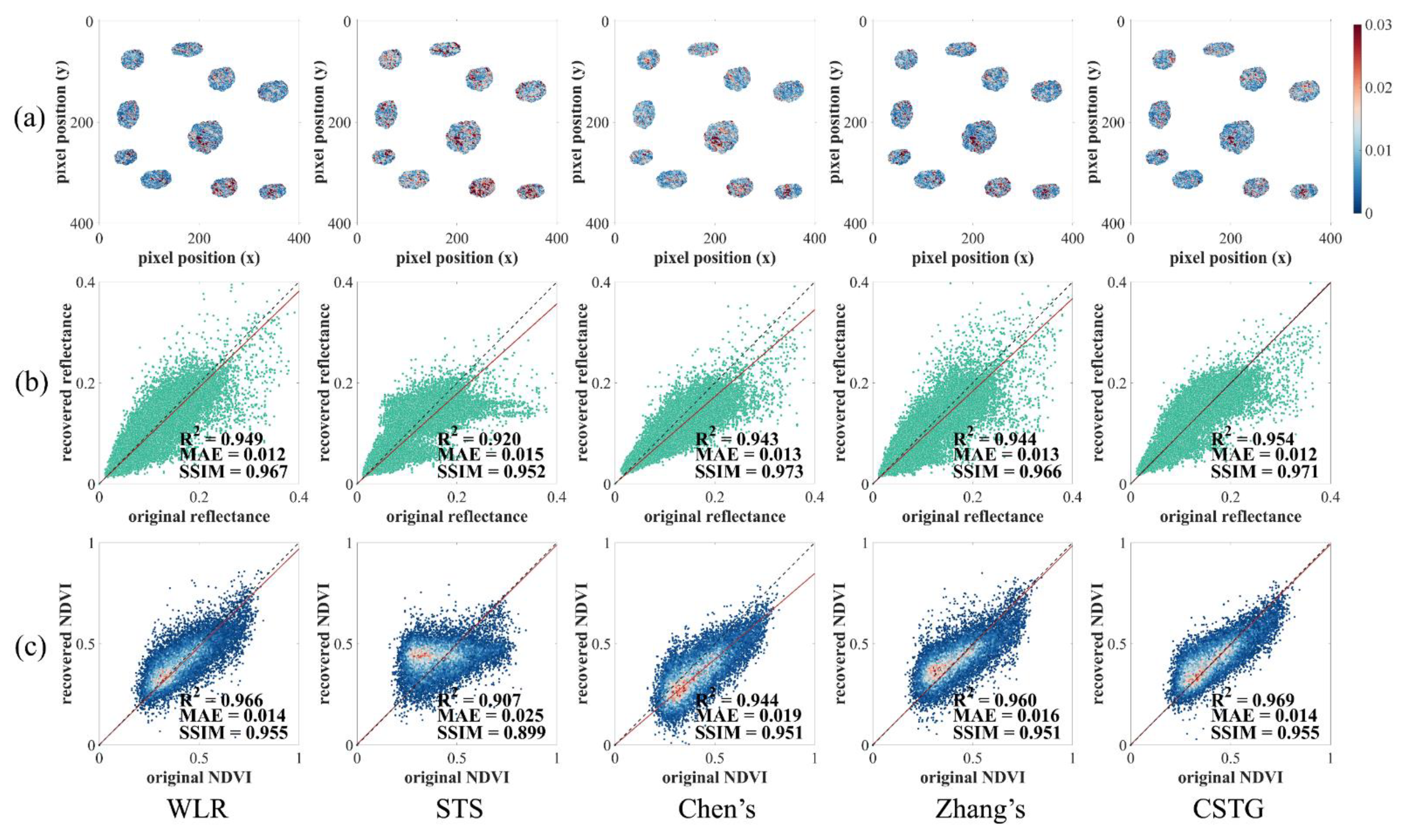
Figure 7a shows the pixel-level error maps, which can reflect the mean reflectance difference of each pixel between the reconstructed maps and the original images of each band. According to the error maps, different methods tend to show miscalculation in similar locations. In addition, there are less areas whose mean errors are over 0.02 (red spots in Figure 7a) in WLR, Zhang’s method and CTSG compared with the other two methods. Scatter plots related to both surface reflectance and normalized difference vegetation index (NDVI) were also derived for the masked areas between the recovered images and the original images. For the surface reflectance in four bands (Figure 7b), WLR, Zhang’s method, and CSTG generated results that are consistent with the original images, where the values range from 0.944 to 0.954, the MAE values range from 0.012 to 0.025, and the SSIM values range from 0.966 to 0.971, respectively. When comparing the NDVI values between the original images and the images recovered using WLR, Zhang’s method, and CSTG (Figure 7c), the values range from 0.960 to 0.969, the MAE values range from 0.014 to 0.016, and the SSIM values range from 0.951 to 0.955, respectively. Both STS and Chen’s method produce images that have slightly lower and higher MAE with the original images than the other three methods. When evaluating individual bands as shown in Table 2, CSTG shows the best performance among the tested methods in Band 1, 2 and 4, where ranges from 0.930 to 0.943, SSIM ranges from 0.950 to 0.958, and MAE ranges from 0.008 to 0.024. Chen’s method shows higher SSIM at most bands and has higher accuracy in Band 3 ( = 0.934, MAE = 0.005, and SSIM = 0.953). According to the metrics of MAE, we found that all the methods show lower values in the visible bands (i.e., Band 1, 3, and 4) than in the near-infrared band (Band 2).
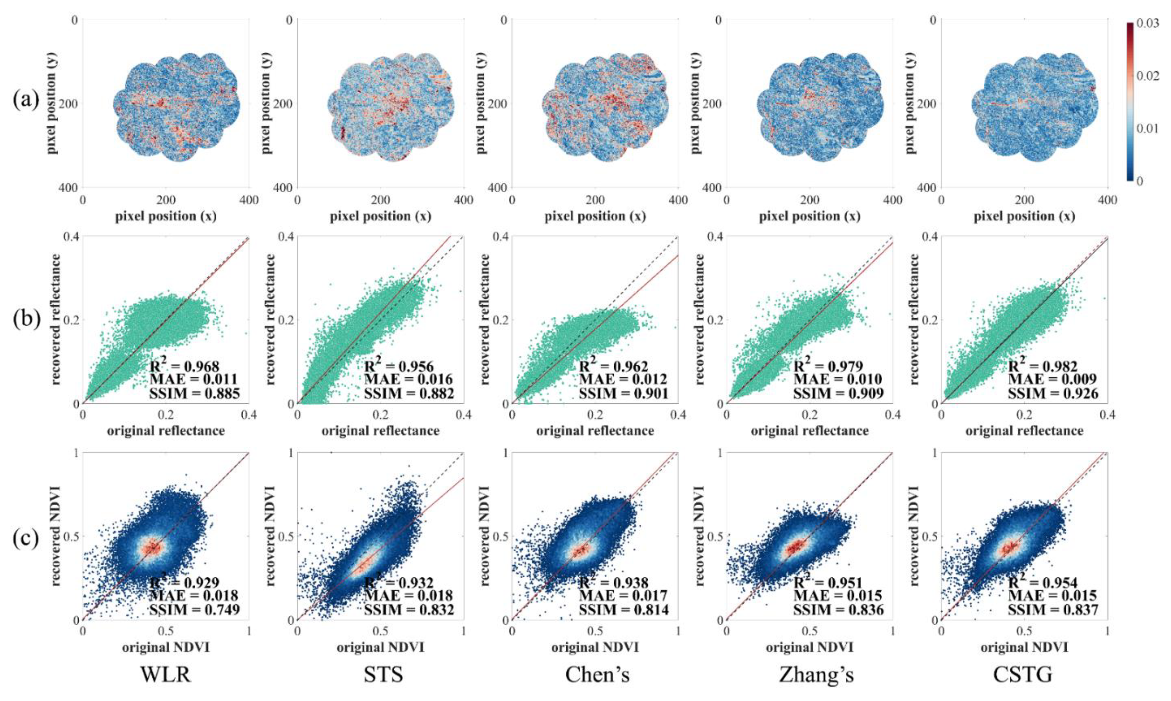
When applying a large and intensive mask, all methods show high similarity in surface reflectance and NDVI between the original images and the recovered images (Figure 8 and Table 3). In addition, it suggests in Figure 8a that Zhang’s method and CSTG provide error maps with lower values in average. In particular, the map derived by CSTG has fewer pixels with values over 0.02 than the other maps, showing a higher accuracy in prediction. For surface reflectance in all bands, Zhang’s method and CSTG exhibit high similarity between the original images and the recovered images, where values are 0.979 and 0.982, MAE values are 0.010 and 0.009, and SSIMs are 0.909 and 0.926, respectively. All models show higher values but lower SSIM values in surface reflectance when applying a large and intensive mask than when applying small and dispersive masks. For individual bands, nearly all models have higher recovery accuracy in the visible bands (Band 1, 3, and 4) than in the near-infrared band (Band 2) as shown in Table 3. The bias in Band 2 reduce the restored accuracy at the large scale. Among all methods, CSTG is able to restore images with consistently high accuracies when applying both large and small masks.
Taking two scenes as examples, Figure 9 displays the recovery results of time series of images with irregularly distributed masks. For images that have few repetitive and overlapped masks in the time series (Figure 9A), both Zhang’s method and CSTG produce reasonably recovered images as compared to the original images in terms of image texture and spectrum in the modestly cloudy areas (Figure 9A, 18 July and 30 September), and Zhang’s method fails to recover some dark shadows in the largely masked areas (Figure 9A, 29 August and 16 October). For images that have considerably repetitive and overlapped masks in time series (Figure 9B), images recovered using Zhang’s method have partial grid-like shades and black shadows after reconstruction, no matter if the masked areas are small (Figure 9B, 5 March and 18 December) or large (Figure 9B, 26 February and 23 April). One possible reason is that Zhang’s method sorts the reference patches according to their integrity. Patches with higher integrity are considered as reliable patches, which are assigned higher weights in calculation. When there are repetitively masked areas in patches that are erroneously considered as reliable, the model will use the masked value as the pixel data for subsequent analysis and generate unsatisfactory results. CSTG improves the performance of image recovery when there are repetitive and overlapped masks in the time series of images and is able to provide reconstructed images reasonably.
Table 4 illustrates the evaluation metrics derived by comparing the surface reflectance in all bands between the original images and the images recovered using different methods. As the and SSIM are designed to evaluate the similarity of the whole images, they are largely affected by the area of the missing regions. Therefore, a decrease in and SSIM shows in both methods when the missing areas extend. Considering the images with small missing areas (scenario A, Image 2 and Image 4), Zhang’s method and CSTG have similar performance according to different metrics. While in larger missing areas (scenario A, Image 1, Image 3 and Image 5), CSTG shows obvious lower MAE, higher and SSIM. According to scenario B, although both Zhang’s method and CSTG have low MAE values when comparing the original images with the recovered images, Zhang’s method has lower (decreased from 0.974 to 0.805) and SSIM values (decreased from 0.965 to 0.911) as the overlap of the masks increases. CSTG still has over 0.94 and SSIM over 0.93 when comparing the recovered images with the original images. The mean values for the evaluation metrics indicate that CSTG generally performs better than Zhang’s method in the two simulated circumstances, and it demonstrates that CSTG is robust for restoring time series of images.
5.2. Experiments Based on Observed Datasets
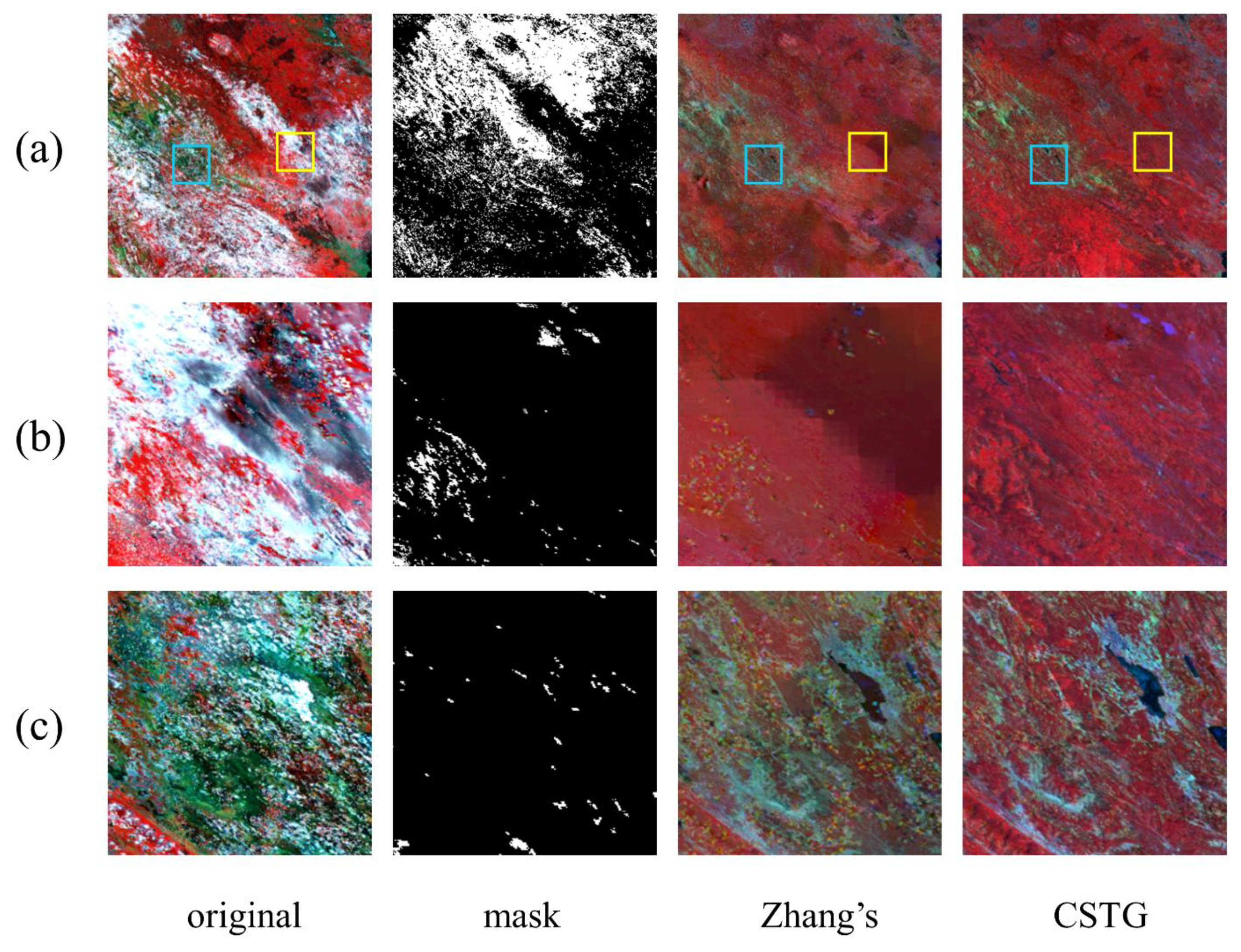
Figure 10 illustrates the images recovered from individual MOD13Q1 images using different methods. Both Zhang’s method and CSTG could remove clouds and restore cloud-free images as compared to the original images. For two zoomed areas as shown in Figure 10b,c, CSTG effectively reduced the spectral noise of the cloudy image and captured the texture details well; however, images recovered using Zhang’s method have jagged grids and missed some texture details.
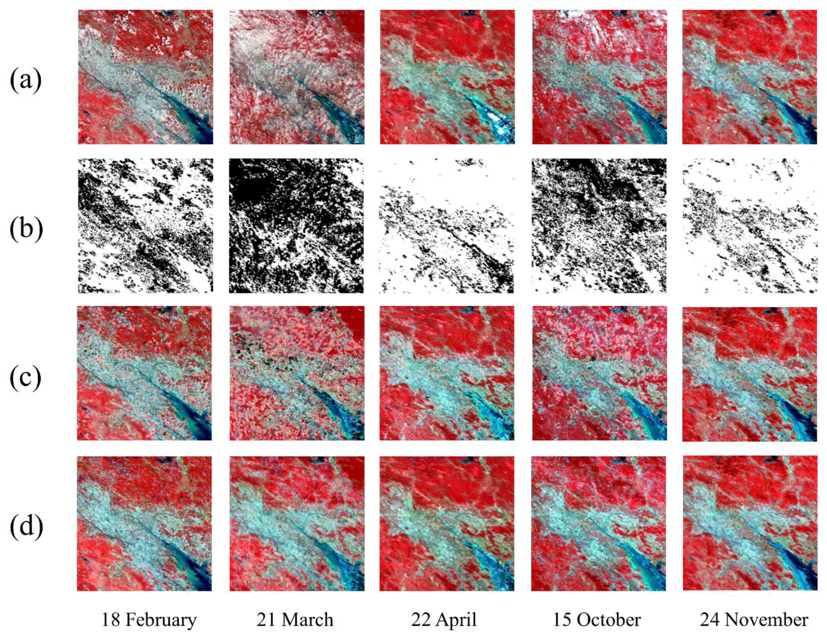
Figure 11 shows the recovery results for time series of images acquired in 2020. Both methods could remove most clouds and restore the contents of the land surface in the time series of images. In areas with little cloud noise, two methods produce relatively consistent recovery results (e.g., 22 April and 24 November). In areas with considerable cloud contamination, CSTG largely reduced the speckle noise in the repetitively cloudy areas and the image fragmentation due to spectral differences (18 February, 21 March, and 15 October) as compared to Zhang’s method. Overall, CSTG performs well on removing clouds and filling image gaps and provides high-quality images in a time series.
5.3. Ablation Study of Sequence-Texture Generation Network
To understand the role of sequence-texture network as proposed in this research, we took the first image in Figure 9B as an example and compared the feature maps generated with and without the sequence-texture generation network. Table 5 shows quantitative metrics evaluated by the model with and without a sequence-generation network. Without a sequence-texture generation network, reduced from 0.959 and 0.962 to 0.870 and 0.896 in image 3 and image 4, respectively, and MAE raised to 0.033 in image 4. This suggests a significant improvement in each image with the sequence-texture generation network according to quantitative metrics, especially in image 1, image 3, and image 4, where missing areas are large and overlapping.
6. Discussion
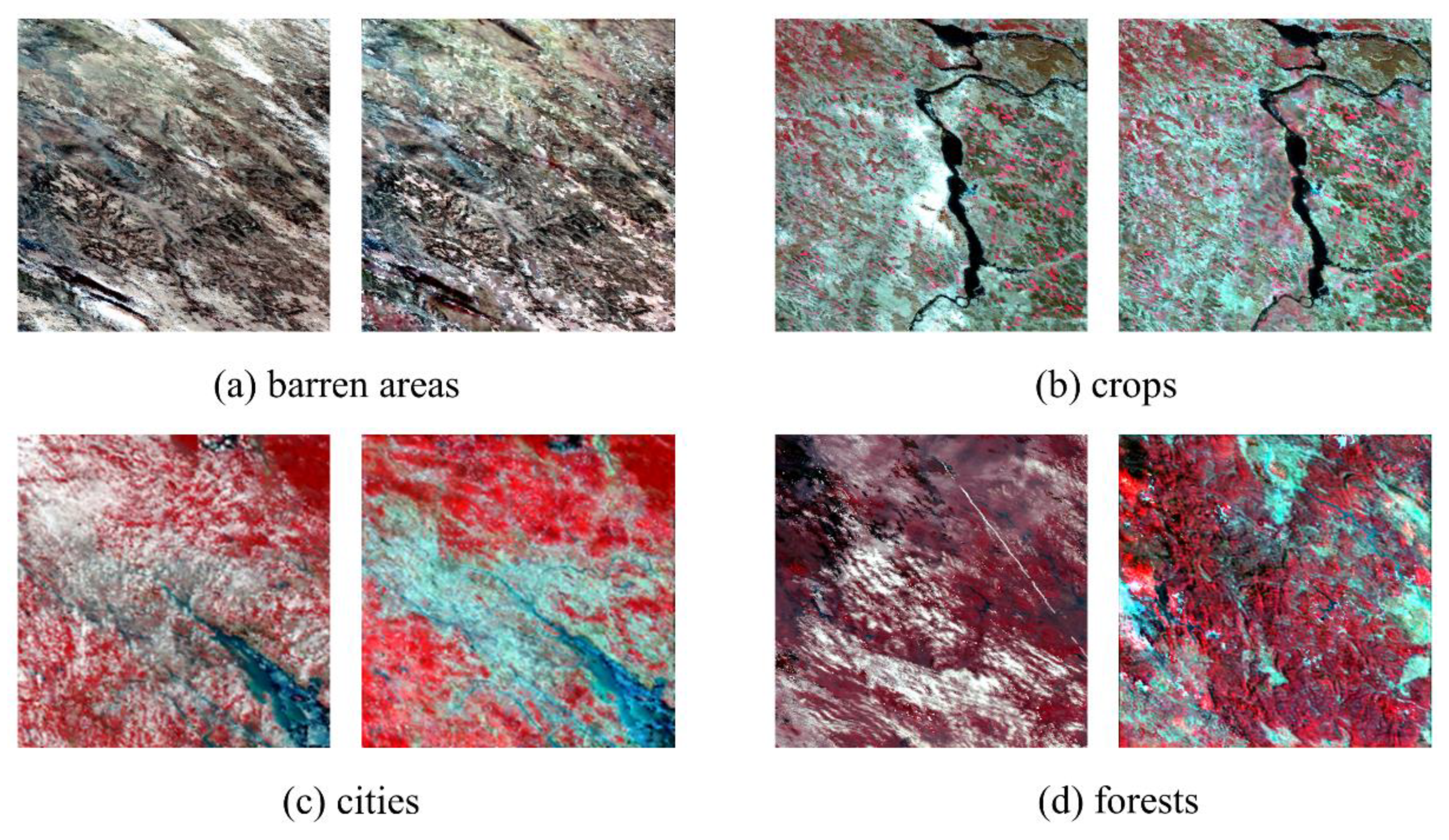
To demonstrate the spatial transferability of CSTG, Figure 12 shows the results of different land surface characteristics with thick clouds recovered by CSTG. It is notable that although the surface characteristics that we did not include in our training data (such as barren areas in Figure 12a) are generated with slight flaws, the results are still acceptable. It also shows that our method could finish gap filling tasks both in vegetation regions (Figure 12b,d) and non-vegetation regions (Figure 12a,c). Even when the cloud cover in the patch window extends to a large area (Figure 12c,d), our method could also reconstruct them and help to get clear textures.
The method proposed in this study can obtain higher accuracy in recovery of both individual images and time series of images, which is predominantly due to abundant temporal information extracted in the networks. Compared to comparison models for individual image reconstruction that can only obtain one temporal image from another time, such as WLR, STS and Chen’s method, our method may obtain more temporal information and the change tendency in time series. WLR considers local similar pixels in spectra and could always obtain recovery results with high spectral similarity with the original images. Some non-local information, such as textures and structures are ignored, so the texture details may be blurred when recovering large missing areas of images. In CSTG, sequence-texture generation network and the structural similarity loss are designed to improve this problem. Additionally, prior spectral noise added in CSTG make sense as it helps the network to obtain more global spectral information than the other deep learning methods. Moreover, compared with the multi-temporal image recovery method, our model can deal with overlapped clouds, as we included this type of situation when we generate random masks in model training. Sequence-texture generation network can also reduce spectral discrepancy caused by overlapping masks. It avoids the situation that mask pixels are also calculated as supplementary data, thus reducing grid-like shades and black shadows.
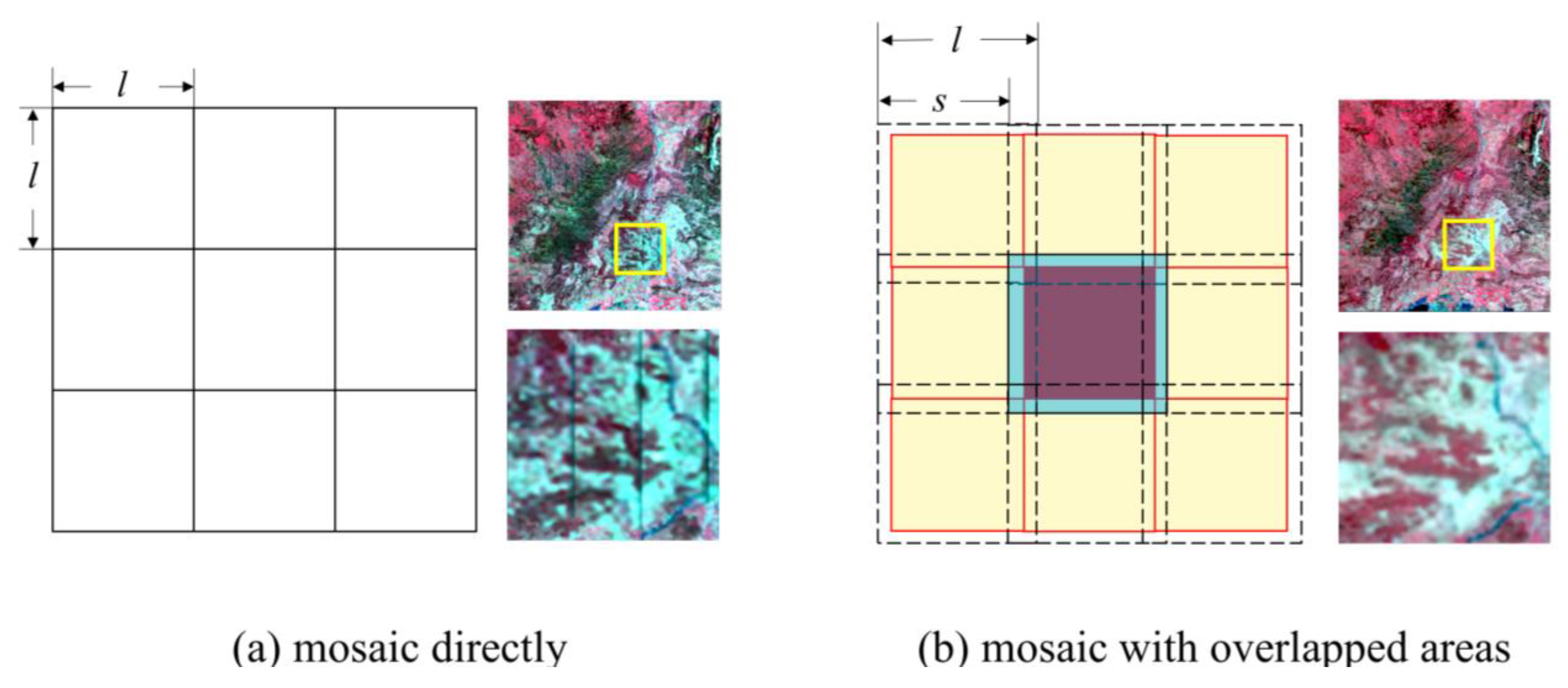
When we perform model prediction, we need to clip large images into smaller patches for recovery and mosaic the recovered patches. As shown in Figure 13, if we splice patches directly without overlap, it may lead to inaccurate predictions in the edge areas (Figure 13a) due to the padding strategy in convolution. To solve this problem, we might clip a patch of size l with stride s (s < l) to make sure there is overlap between adjacent images. By abandoning the edge areas with a size of (l − s)/2 in each patch, we are able to reconstruct a large image without block effects as shown in Figure 13b.
As the proposed framework includes two parts of networks, our experiments take a slightly longer time to train and test the model than Zhang’s method. It took 25 h to train the model and 117.9 s to predict the final results of Figure 9A. In comparison, for Zhang’s method, it only took 21 h for fitting the model and 72.2 s for prediction. It is also notable that the prediction time efficiency of the proposed method only depends on the size of the testing images and the performance of GPU. The prediction time of Zhang’s method is also influenced by the mask areas of each image. This suggests that the proposed model is more applicable for the situation where the missing areas are large and a higher accuracy is needed. We will learn further about the existing reconstruction models with high time efficiency and try to shorten the running time of our model in the future.
The method proposed in this study aims to restore long time series of MODIS data that often have repetitive and overlapping clouds. The method needs high-quality images for the training sets and it is difficult to find an area that has completely cloud-free MODIS data throughout the entire time series, thus it is still challenging to restore long time series images. To overcome the above-mentioned problem, we might first train a model with a relatively short time sequence and use the model repetitively to recover the cloudy areas for a given year, and further use the recovered yearly data as a training set to recover the cloudy data in the long time series. In this way, the method proposed in this study has the potential to reconstruct long time series of remote sensing data. The experiments for a broad application of the developed method are beyond the scope of this study and we will conduct them in further studies. Additionally, we screened out poor-quality pixels in the images based on the quality of data provided in the MODIS product, which includes some high-quality pixels and we may miss some useful information. If each image in the time series has a very large proportion of areas with poor-quality observations, the developed method might not perform well as the network does not receive correct information. In addition, the current network structure consists of both the content generation network and the sequence-texture generation network, and we aim to develop an end-to-end network in our future research.
7. Conclusions
As existing studies have difficulty processing time series of remote sensing images with missing data, we proposed a content-sequence-texture generation (CSTG) network to gap-fill time series of satellite images. The method combines a content generation network and a sequence-texture generation network for recovering time series of remote sensing images with missing data. We evaluated the performance of CSTG using time series of MODIS data and compared it with four existing methods. The results indicate that CSTG has higher accuracy when restoring images with large and overlapping masks. Comparing the surface reflectance between the original images and the images recovered using CSTG, , MAE, and SSIM are 0.954, 0.012, and 0.971, respectively, when applying small and dispersive masks, and , MAE, and SSIM are 0.982, 0.009, and 0.926, respectively, when applying a large and intensive mask. The model is robust to time series of images that have overlapping cloudy areas. The method highlights the potential of the deep learning methods on reconstructing remote sensing images to provide high-quality time series data for downstream applications.
Author Contributions
Conceptualization, Y.W., Z.A. and Q.X.; methodology, Y.W., Z.A. and Q.X.; software, Y.W.; validation, Y.W., K.X. and C.Y.; formal analysis, Y.W.; writing—original draft preparation, Y.W. and X.Z.; writing—review and editing, X.Z., Z.A. and Q.X.; visualization, Y.W., K.X. and C.Y.; supervision, Q.X.; funding acquisition, Q.X. All authors have read and agreed to the published version of the manuscript.
Funding
This research is supported by National Natural Science Foundation of China (grant nos. 41875122 and U1811464), National Key R&D Program of China (grant nos. 2017YFA0604300 and 2017YFA0604400), Western Talents (grant no. 2018XBYJRC004), Guangdong Top Young Talents (grant no. 2017TQ04Z359). We thank anonymous reviewers for their constructive comments.
Data Availability Statement
MODIS data used for training, validation, and testing are available at https://ladsweb.modaps.eosdis.nasa.gov/search/order (accessed on 15 October 2020).
Acknowledgments
We sincerely thank the researchers and investigators in the comparison methods for providing available software and codes.
Conflicts of Interest
The authors declare no conflict of interest.
References
- Di Vittorio, C.A.; Georgakakos, A.P. Land cover classification and wetland inundation mapping using modis. Remote Sens. Environ. 2018, 204, 1–17. [Google Scholar] [CrossRef]
- Vali, A.; Comai, S.; Matteucci, M. Deep learning for land use and land cover classification based on hyperspectral and multispectral earth observation data: A review. Remote Sens. 2020, 12, 2495. [Google Scholar] [CrossRef]
- Li, Z.; Xin, Q.; Sun, Y.; Cao, M. A deep learning-based framework for automated extraction of building footprint polygons from very high-resolution aerial imagery. Remote Sens. 2021, 13, 3630. [Google Scholar] [CrossRef]
- Xin, Q.C.; Dai, Y.J.; Liu, X.P. A simple time-stepping scheme to simulate leaf area index, phenology, and gross primary production across deciduous broadleaf forests in the eastern united states. Biogeosciences 2019, 16, 467–484. [Google Scholar] [CrossRef]
- Wu, W.; Sun, Y.; Xiao, K.; Xin, Q. Development of a global annual land surface phenology dataset for 1982–2018 from the avhrr data by implementing multiple phenology retrieving methods. Int. J. Appl. Earth Obs. 2021, 103, 102487. [Google Scholar] [CrossRef]
- Omori, K.; Sakai, T.; Miyamoto, J.; Itou, A.; Oo, A.N.; Hirano, A. Assessment of paddy fields’ damage caused by cyclone nargis using modis time-series images (2004–2013). Paddy Water Environ. 2021, 19, 271–281. [Google Scholar] [CrossRef]
- Yokoya, N.; Yamanoi, K.; He, W.; Baier, G.; Adriano, B.; Miura, H.; Oishi, S. Breaking limits of remote sensing by deep learning from simulated data for flood and debris-flow mapping. IEEE Trans. Geosci. Remote Sens. 2022, 60, 4400115. [Google Scholar] [CrossRef]
- Chen, S.; Chen, X.; Chen, X.; Chen, J.; Cao, X.; Shen, M.; Yang, W.; Cui, X. A novel cloud removal method based on ihot and the cloud trajectories for landsat imagery. Remote Sens. 2018, 10, 1040. [Google Scholar] [CrossRef]
- Shen, H.; Li, H.; Qian, Y.; Zhang, L.; Yuan, Q. An effective thin cloud removal procedure for visible remote sensing images. ISPRS J. Photogramm. Remote Sens. 2014, 96, 224–235. [Google Scholar] [CrossRef]
- Richter, R. Atmospheric correction of satellite data with haze removal including a haze/clear transition region. Comput. Geosci. 1996, 22, 675–681. [Google Scholar] [CrossRef]
- Guillemot, C.; Le Meur, O. Image inpainting: Overview and recent advances. IEEE Signal Proc. Mag. 2014, 31, 127–144. [Google Scholar] [CrossRef]
- Sadiq, A.; Sulong, G.; Edwar, L. Recovering defective landsat 7 enhanced thematic mapper plus images via multiple linear regression model. IET Comput. Vis. 2016, 10, 788–797. [Google Scholar] [CrossRef]
- Pringle, M.J.; Schmidt, M.; Muir, J.S. Geostatistical interpolation of slc-off landsat etm plus images. ISPRS J. Photogramm. Remote Sens. 2009, 64, 654–664. [Google Scholar] [CrossRef]
- Zhang, C.R.; Li, W.D.; Civco, D. Application of geographically weighted regression to fill gaps in slc-off landsat etm plus satellite imagery. Int. J. Remote Sens. 2014, 35, 7650–7672. [Google Scholar] [CrossRef]
- Cheng, Q.; Shen, H.F.; Zhang, L.P.; Yuan, Q.Q.; Zeng, C. Cloud removal for remotely sensed images by similar pixel replacement guided with a spatio-temporal mrf model. ISPRS J. Photogramm. Remote Sens. 2014, 92, 54–68. [Google Scholar] [CrossRef]
- Yang, J.F.; Yin, W.T.; Zhang, Y.; Wang, Y.H. A fast algorithm for edge-preserving variational multichannel image restoration. SIAM J. Imaging Sci. 2009, 2, 569–592. [Google Scholar] [CrossRef]
- Wang, Q.; Wang, L.; Li, Z.; Tong, X.; Atkinson, P.M. Spatial–spectral radial basis function-based interpolation for landsat etm+ slc-off image gap filling. IEEE Trans. Geosci. Remote Sens. 2021, 59, 7901–7917. [Google Scholar] [CrossRef]
- Lin, C.H.; Tsai, P.H.; Lai, K.H.; Chen, J.Y. Cloud removal from multitemporal satellite images using information cloning. IEEE Trans. Geosci. Remote Sens. 2013, 51, 232–241. [Google Scholar] [CrossRef]
- Shen, Y.; Wang, Y.; Lv, H.T.; Qian, J. Removal of thin clouds in landsat-8 oli data with independent component analysis. Remote Sens. 2015, 7, 11481–11500. [Google Scholar] [CrossRef]
- Makarau, A.; Richter, R.; Schlapfer, D.; Reinartz, P. Combined haze and cirrus removal for multispectral imagery. IEEE Geosci. Remote Sens. Lett. 2016, 13, 379–383. [Google Scholar] [CrossRef]
- Zhang, Y.; Guindon, B.; Cihlar, J. An image transform to characterize and compensate for spatial variations in thin cloud contamination of landsat images. Remote Sens. Environ. 2002, 82, 173–187. [Google Scholar] [CrossRef]
- Gladkova, I.; Grossberg, M.D.; Shahriar, F.; Bonev, G.; Romanov, P. Quantitative restoration for modis band 6 on aqua. IEEE Trans. Geosci. Remote Sens. 2012, 50, 2409–2416. [Google Scholar] [CrossRef]
- Xin, Q.C.; Olofsson, P.; Zhu, Z.; Tan, B.; Woodcock, C.E. Toward near real-time monitoring of forest disturbance by fusion of modis and landsat data. Remote Sens. Environ. 2013, 135, 234–247. [Google Scholar] [CrossRef]
- Wang, Y.; Yuan, Q.Q.; Li, T.W.; Shen, H.F.; Zheng, L.; Zhang, L.P. Large-scale modis aod products recovery: Spatial-temporal hybrid fusion considering aerosol variation mitigation. ISPRS J. Photogramm. Remote Sens. 2019, 157, 1–12. [Google Scholar] [CrossRef]
- Roy, D.P.; Ju, J.; Lewis, P.; Schaaf, C.; Gao, F.; Hansen, M.; Lindquist, E. Multi-temporal modis-landsat data fusion for relative radiometric normalization, gap filling, and prediction of landsat data. Remote Sens. Environ. 2008, 112, 3112–3130. [Google Scholar] [CrossRef]
- Moreno-Martínez, Á.; Izquierdo-Verdiguier, E.; Maneta, M.P.; Camps-Valls, G.; Robinson, N.; Muñoz-Marí, J.; Sedano, F.; Clinton, N.; Running, S.W. Multispectral high resolution sensor fusion for smoothing and gap-filling in the cloud. Remote Sens. Environ. 2020, 247, 111901. [Google Scholar] [CrossRef] [PubMed]
- Hu, C.; Huo, L.; Zhang, Z.; Tang, P. Multi-temporal landsat data automatic cloud removal using poisson blending. IEEE Access 2020, 8, 46151–46161. [Google Scholar] [CrossRef]
- Tseng, D.C.; Tseng, H.T.; Chien, C.L. Automatic cloud removal from multi-temporal spot images. Appl. Math. Comput. 2008, 205, 584–600. [Google Scholar] [CrossRef]
- Chen, J.; Zhu, X.L.; Vogelmann, J.E.; Gao, F.; Jin, S.M. A simple and effective method for filling gaps in landsat etm plus slc-off images. Remote Sens. Environ. 2011, 115, 1053–1064. [Google Scholar] [CrossRef]
- Zeng, C.; Shen, H.F.; Zhang, L.P. Recovering missing pixels for landsat etm plus slc-off imagery using multi-temporal regression analysis and a regularization method. Remote Sens. Environ. 2013, 131, 182–194. [Google Scholar] [CrossRef]
- Goodfellow, I.J.; Pouget-Abadie, J.; Mirza, M.; Xu, B.; Warde-Farley, D.; Ozair, S.; Courville, A.; Bengio, Y. Generative adversarial nets. In Proceedings of the 27th International Conference on Neural Information Processing Systems, Montreal, QC, Canada, 8–13 December 2014; MIT Press: Cambridge, MA, USA, 2014; Volume 2, pp. 2672–2680. [Google Scholar]
- Zhang, H.; Xu, T.; Li, H.; Zhang, S.; Wang, X.; Huang, X.; Metaxas, D. Stackgan: Text to photo-realistic image synthesis with stacked generative adversarial networks. In Proceedings of the 2017 IEEE International Conference on Computer Vision (ICCV), Venice, Italy, 22–29 October 2017; pp. 5908–5916. [Google Scholar]
- Zhu, J.; Park, T.; Isola, P.; Efros, A.A. Unpaired image-to-image translation using cycle-consistent adversarial networks. In Proceedings of the 2017 IEEE International Conference on Computer Vision (ICCV), Venice, Italy, 22–29 October 2017; pp. 2242–2251. [Google Scholar]
- Chen, Y.; Tang, L.L.; Yang, X.; Fan, R.S.; Bilal, M.; Li, Q.Q. Thick clouds removal from multitemporal zy-3 satellite images using deep learning. IEEE J. Sel. Topics Appl. Earth Observ. Remote Sens. 2019, 13, 143–153. [Google Scholar] [CrossRef]
- Zhang, Q.; Yuan, Q.Q.; Li, J.; Li, Z.W.; Shen, H.F.; Zhang, L.P. Thick cloud and cloud shadow removal in multitemporal imagery using progressively spatio-temporal patch group deep learning. ISPRS J. Photogramm. Remote Sens. 2020, 162, 148–160. [Google Scholar] [CrossRef]
- Li, W.; Li, Y.; Chan, J.C.W. Thick cloud removal with optical and sar imagery via convolutional-mapping-deconvolutional network. IEEE Trans. Geosci. Remote Sens. 2020, 58, 2865–2879. [Google Scholar] [CrossRef]
- Zhu, Z.; Wang, S.X.; Woodcock, C.E. Improvement and expansion of the fmask algorithm: Cloud, cloud shadow, and snow detection for landsats 4-7, 8, and sentinel 2 images. Remote Sens. Environ. 2015, 159, 269–277. [Google Scholar] [CrossRef]
- Li, Z.W.; Shen, H.F.; Cheng, Q.; Liu, Y.H.; You, S.C.; He, Z.Y. Deep learning based cloud detection for medium and high resolution remote sensing images of different sensors. ISPRS J. Photogramm. Remote Sens. 2019, 150, 197–212. [Google Scholar] [CrossRef]
- Shi, X.; Chen, Z.; Wang, H.; Yeung, D.Y.; Wong, W.K.; Woo, W.C. Convolutional Lstm Network: A Machine Learning Approach for Precipitation Nowcasting; MIT Press: Cambridge, MA, USA, 2015. [Google Scholar]
- Si, C.; Chen, W.; Wang, W.; Wang, L.; Tan, T. An attention enhanced graph convolutional lstm network for skeleton-based action recognition. In Proceedings of the IEEE/CVF Conference on Computer Vision and Pattern Recognition, Long Beach, CA, USA, 15–20 June 2019; pp. 1227–1236. [Google Scholar]
- Kingma, D.; Ba, J. Adam: A method for stochastic optimization. arXiv 2014, arXiv:1412.6980. [Google Scholar]
- Zhang, Q.; Yuan, Q.; Chao, Z.; Li, X.; Wei, Y. Missing data reconstruction in remote sensing image with a unified spatial-temporal-spectral deep convolutional neural network. IEEE Trans. Geosci. Remote Sens. 2018, 56, 4274–4288. [Google Scholar] [CrossRef] [Green Version]
Figure 1.
The spatial distribution of the study areas and the study data.

Figure 2.
The flowchart of the proposed recovery method. The first line shows the model training process, and the second line shows the model testing process.
Figure 2.
The flowchart of the proposed recovery method. The first line shows the model training process, and the second line shows the model testing process.

Figure 3.
The structure of the content generation network proposed in this study.

Figure 4.
The structure of (a) the sequence-texture generation networks proposed in this study, (b) the ConvLSTM cell.
Figure 4.
The structure of (a) the sequence-texture generation networks proposed in this study, (b) the ConvLSTM cell.

Figure 5.
Comparisons of the observed images and the gap-filled images when applying small and dispersive masks are shown for (a) the original image acquired on 30 September 2020, (b) the image with artificial masks, (c) the supplementary image acquired on 8 October 2020, and the images recovered by (d) WLR, (e) STS, (f) Chen’s method, (g) Zhang’s method, and (h) CSTG.

Figure 6.
Comparisons of the observed images and the gap-filled images when applying a large and intensive mask are shown for (a) the original image acquired on 26 February 2019, (b) the image with artificial masks, (c) the supplementary image acquired on 29 August 2019, and the images recovered by (d) WLR, (e) STS, (f) Chen’s method, (g) Zhang’s method, and (h) CSTG.

Figure 7.
Visualization maps of quantitative analysis between recovered and original values using different methods at small and dispersive missing areas: (a) pixel-level error maps; (b) the regression analysis of the normalized reflectance; (c) the regression analysis of the NDVI. In (b,c), the solid red lines denote the regression lines and the dashed black lines denote the 1:1 lines.

Figure 8.
Visualization maps of quantitative analysis between recovered and original values using different methods with a large and intensive mask area: (a) pixel-level error maps; (b) regression analysis of the normalized reflectance; (c) regression analysis of the NDVI. In (b,c), the solid red lines denote the regression lines and the dashed black lines denote the 1:1 lines.

Figure 9.
The time series of images are shown for (a) the original data, (b) the simulated masks, (c) the recovery results using Zhang’s method, and (d) the recovery results using CSTG. (A,B) are two different scenes to simulate large missing areas and overlapped missing areas respectively. The original images were acquired in 2017 and 2020, respectively.

Figure 10.
Recovery results for an individual image using different methods are shown for (a) the entire images, (b) the zoomed-in images as marked by the yellow rectangle in (a), and (c) the zoomed-in images as marked by the blue rectangle in (a). The black parts masks are cloudy areas and the white parts are cloud-free areas.

Figure 11.
Recovery results of time series images based on different methods. (a) Original images. (b) Quality detection (The black parts are cloudy areas and the white parts are cloud-free areas). (c) Results of Zhang’s method. (d) Results of the CSTG method. The original images were acquired in 2020.

Figure 12.
Reconstruction results of CSTG with different surface characteristics.

Figure 13.
The comparison for images to process large images using the methods that (a) mosaic image patches directly, and (b) mosaic image patches with overlapping areas in the edges.
Figure 13.
The comparison for images to process large images using the methods that (a) mosaic image patches directly, and (b) mosaic image patches with overlapping areas in the edges.


Table 1.
MODIS product (MOD09A1 and MOD13Q1) instances in this study.
| Data Usage | Site Location | MODIS Tile ID | Product Type | Longitude and Latitude | Date Ranges |
|---|---|---|---|---|---|
| Training data | North America | H12V04 | MOD09A1 | 74.315°W–79.478°W, 39.927°N–41.615°N | 1 January 2016–31 December 2016 |
| Europe | H19V03 | MOD09A1 | 15.667°E–19.12°E 51.068°N–52.737°N | ||
| Asia | H27V05 | MOD09A1 | 107.888°E–112.234°E 32.985°N–34.674°N | ||
| H27V05 | MOD09A1 | 111.881°E–116.068°E 31.808°N–33.485°N | |||
| H27V06 | MOD13Q1 | 98.310°E–99.71°E 21.793°N–22.476°N | |||
| Validation data | North America | H12V04 | MOD09A1 | 80.721°W–85.922°W 41.004°N–42.686°N | 1 January 2017–31 December 2017 |
| Europe | H19V03 | MOD13Q1 | 25.503°E–27.437°E 54.832°N–55.658°N | ||
| Test data | North America | H12V04 | MOD09A1 | 71.618°W–75.790°W 41.251°N–42.615°N | 10 June 2017, 18 July 2017, 29 August 2017, 30 September 2017, 16 October 2017 |
| Europe | H19V03 | MOD09A1 | 18.404°E–20.379°E 51.252°N–52.915°N | 16 September 2020–14 October 2020 | |
| H20V03 | MOD09A1 | 34.639°E–36.013°E 50.002°N–51.665°N | 12 February 2019–12 March 2019, 29 August 2019 | ||
| Asia | H27V06 | MOD13Q1 | 99.366°E–99.986°E 22.801°N–22.632°N | 2 February 2020, 5 March 2020, 31 October 2020, 16 November 2020, 18 December 2020 | |
| H27V06 | MOD13Q1 | 103.088°E–106.084°E 20.002°N–29.167°N | 11 June 2019–9 July 2019 | ||
| H28V06 | MOD09A1 | 113.367°E–113.775°E 22.152°N–22.632°N | 18 February 2020, 21 March 2020, 22 April 2020, 15 October 2020, 24 November 2020 |
Table 2.
The evaluation metrics for four individual bands in the masked areas between the original images obtained from MOD09A1 and the images recovered using different methods. Small and dispersive masks were applied to the original images. The values in bold are the best values for each metric.
Table 2.
The evaluation metrics for four individual bands in the masked areas between the original images obtained from MOD09A1 and the images recovered using different methods. Small and dispersive masks were applied to the original images. The values in bold are the best values for each metric.
| Methods | Band 1 | Band 2 | Band 3 | Band 4 | ||||||||
|---|---|---|---|---|---|---|---|---|---|---|---|---|
| R2 | MAE | SSIM | R2 | MAE | SSIM | R2 | MAE | SSIM | R2 | MAE | SSIM | |
| WLR | 0.925 | 0.011 | 0.948 | 0.933 | 0.024 | 0.950 | 0.925 | 0.006 | 0.938 | 0.915 | 0.008 | 0.943 |
| STS | 0.894 | 0.014 | 0.924 | 0.890 | 0.032 | 0.913 | 0.907 | 0.006 | 0.919 | 0.894 | 0.009 | 0.922 |
| Chen’s | 0.930 | 0.011 | 0.960 | 0.914 | 0.027 | 0.949 | 0.934 | 0.005 | 0.953 | 0.928 | 0.008 | 0.958 |
| Zhang’s | 0.915 | 0.012 | 0.946 | 0.928 | 0.025 | 0.949 | 0.919 | 0.006 | 0.938 | 0.908 | 0.008 | 0.941 |
| CSTG | 0.943 | 0.010 | 0.958 | 0.938 | 0.024 | 0.951 | 0.932 | 0.006 | 0.950 | 0.930 | 0.008 | 0.952 |
Table 3.
The evaluate metrics between recovered reflectance values using different methods and original reflectance values derived from MOD09A1 for single band at large missing areas. A large and intensive mask was applied to the original images. The values in bold are the best values for each metric.
| Methods | B1 | B2 | B3 | B4 | ||||||||
|---|---|---|---|---|---|---|---|---|---|---|---|---|
| R2 | MAE | SSIM | R2 | MAE | SSIM | R2 | MAE | SSIM | R2 | MAE | SSIM | |
| WLR | 0.861 | 0.009 | 0.871 | 0.681 | 0.025 | 0.740 | 0.855 | 0.005 | 0.917 | 0.889 | 0.006 | 0.912 |
| STS | 0.813 | 0.012 | 0.863 | 0.794 | 0.020 | 0.848 | 0.765 | 0.007 | 0.831 | 0.787 | 0.008 | 0.874 |
| Chen’s | 0.783 | 0.012 | 0.897 | 0.813 | 0.023 | 0.783 | 0.875 | 0.004 | 0.930 | 0.868 | 0.007 | 0.921 |
| Zhang’s | 0.849 | 0.010 | 0.886 | 0.821 | 0.018 | 0.821 | 0.856 | 0.005 | 0.923 | 0.886 | 0.006 | 0.920 |
| CSTG | 0.877 | 0.009 | 0.905 | 0.860 | 0.016 | 0.870 | 0.860 | 0.005 | 0.928 | 0.868 | 0.007 | 0.924 |
Table 4.
The evaluate metrics derived by comparing the surface reflectance in all bands between the original images and the images recovered using different methods. The original images come from MOD09A1 and MOD13Q1, respectively.
Table 4.
The evaluate metrics derived by comparing the surface reflectance in all bands between the original images and the images recovered using different methods. The original images come from MOD09A1 and MOD13Q1, respectively.
| Methods | Zhang’s | CSTG | ||||||||||
|---|---|---|---|---|---|---|---|---|---|---|---|---|
| Scenario A | Scenario B | Scenario A | Scenario B | |||||||||
| R2 | MAE | SSIM | R2 | MAE | SSIM | R2 | MAE | SSIM | R2 | MAE | SSIM | |
| Image 1 | 0.967 | 0.018 | 0.913 | 0.947 | 0.016 | 0.944 | 0.971 | 0.017 | 0.900 | 0.986 | 0.011 | 0.958 |
| Image 2 | 0.982 | 0.013 | 0.986 | 0.974 | 0.015 | 0.965 | 0.987 | 0.013 | 0.986 | 0.978 | 0.014 | 0.970 |
| Image 3 | 0.948 | 0.017 | 0.898 | 0.946 | 0.013 | 0.929 | 0.965 | 0.015 | 0.930 | 0.959 | 0.010 | 0.931 |
| Image 4 | 0.979 | 0.010 | 0.990 | 0.805 | 0.043 | 0.911 | 0.985 | 0.009 | 0.993 | 0.962 | 0.024 | 0.934 |
| Image 5 | 0.937 | 0.013 | 0.934 | 0.959 | 0.020 | 0.968 | 0.968 | 0.010 | 0.950 | 0.947 | 0.023 | 0.970 |
| Mean | 0.963 | 0.014 | 0.944 | 0.926 | 0.021 | 0.943 | 0.975 | 0.013 | 0.952 | 0.966 | 0.016 | 0.953 |
Table 5.
Quantitative results of ablation study of sequence-texture generation network.
| Method | Image 1 R2/MAE/SSIM | Image 2 R2/MAE/SSIM | Image 3 R2/MAE/SSIM | Image 4 R2/MAE/SSIM | Image 5 R2/MAE/SSIM |
|---|---|---|---|---|---|
| Without sequence-texture generation | 0.957/0.016/0.951 | 0.979/0.014/0.968 | 0.870/0.027/0.929 | 0.896/0.033/0.914 | 0.900/0.028/0.967 |
| With sequence-texture generation | 0.986/0.011/0.958 | 0.978/0.014/0.970 | 0.959/0.010/0.931 | 0.962/0.024/0.934 | 0.947/0.023/0.970 |
Publisher’s Note: MDPI stays neutral with regard to jurisdictional claims in published maps and institutional affiliations. |
© 2022 by the authors. Licensee MDPI, Basel, Switzerland. This article is an open access article distributed under the terms and conditions of the Creative Commons Attribution (CC BY) license (https://creativecommons.org/licenses/by/4.0/).
Share and Cite
MDPI and ACS Style
Wang, Y.; Zhou, X.; Ao, Z.; Xiao, K.; Yan, C.; Xin, Q. Gap-Filling and Missing Information Recovery for Time Series of MODIS Data Using Deep Learning-Based Methods. Remote Sens. 2022, 14, 4692. https://doi.org/10.3390/rs14194692
AMA Style
Wang Y, Zhou X, Ao Z, Xiao K, Yan C, Xin Q. Gap-Filling and Missing Information Recovery for Time Series of MODIS Data Using Deep Learning-Based Methods. Remote Sensing. 2022; 14(19):4692. https://doi.org/10.3390/rs14194692
Chicago/Turabian StyleWang, Yidan, Xuewen Zhou, Zurui Ao, Kun Xiao, Chenxi Yan, and Qinchuan Xin. 2022. "Gap-Filling and Missing Information Recovery for Time Series of MODIS Data Using Deep Learning-Based Methods" Remote Sensing 14, no. 19: 4692. https://doi.org/10.3390/rs14194692
Note that from the first issue of 2016, this journal uses article numbers instead of page numbers. See further details here.