Article

Assessing the Performance of the South American Land Data Assimilation System Version 2 (SALDAS-2) Energy Balance across Diverse Biomes

by
Álvaro Vasconcellos Araujo de Ávila
1,*,
Luis Gustavo Gonçalves de Gonçalves
2,*,
Vanessa de Arruda Souza
3,4,
Laurizio Emanuel Ribeiro Alves
1,
Giovanna Deponte Galetti
1,
Bianca Muss Maske
1,
Augusto Getirana
5,
Anderson Ruhoff
3,
Marcelo Sacardi Biudes
6,
Nadja Gomes Machado
7 and
Débora Regina Roberti
4
1
Centro de Previsão de Tempo e Estudos Climáticos (CPTEC), Instituto Nacional de Pesquisas Espaciais (INPE), Cachoeira Paulista 12630-000, Brazil
2
Fondazione Centro Euro-Mediterraneo sui Cambiamenti Climatici (CMCC), 40127 Bologna, Italy
3
Instituto de Pesquisas Hidráulicas, Universidade Federal do Rio Grande do Sul (UFRGS), Porto Alegre 91501-970, Brazil
4
Departamento de Física, Universidade Federal de Santa Maria (UFSM), Santa Maria 97105-900, Brazil
5
Hydrological Sciences Laboratory, NASA Goddard Space Flight Center, Greenbelt, MD 20771, USA
6
Instituto de Física, Universidade Federal de Mato Grosso (UFMT), Cuiabá 78060-900, Brazil
7
Instituto Federal de Educação, Ciência e Tecnologia de Mato Grosso (IFMT), Cuiabá 78005-390, Brazil
*
Authors to whom correspondence should be addressed.
Atmosphere 2023, 14(6), 959; https://doi.org/10.3390/atmos14060959
Submission received: 21 March 2023 / Revised: 19 April 2023 / Accepted: 28 April 2023 / Published: 31 May 2023
(This article belongs to the Special Issue Weather and Climate Extremes: Observations, Modeling, and Impacts)

Abstract

:
Understanding the exchange of energy between the surface and the atmosphere is important in view of the climate scenario. However, it becomes a challenging task due to a sparse network of observations. This study aims to improve the energy balance estimates for the Amazon, Cerrado, and Pampa biomes located in South America using the radiation and precipitation forcing obtained from the Clouds and the Earth’s Radiant Energy System (CERES) and the precipitation CPTEC/MERGE datasets. We employed three surface models—Noah-MP, Community Land Model (CLSM), and Integrated Biosphere Simulator (IBIS)—and conducted modeling experiments, termed South America Land Data Assimilation System (SALDAS-2). The results showed that SALDAS-2 radiation estimates had the smallest errors. Moreover, SALDAS-2 precipitation estimates were better than the Global Land Data Assimilation System (GLDAS) in the Cerrado (MBE = −0.16) and Pampa (MBE = −0.19). Noah-MP presented improvements compared with CLSM and IBIS in 100% of towers located in the Amazon. CLSM tends to overestimate the latent heat flux and underestimate the sensible heat flux in the Amazon. Noah-MP and Ensemble outperformed GLDAS in terms latent and sensible heat fluxes. The potential of SALDAS-2 should be emphasized to provide more accurate estimates of surface energy balance.

1. Introduction

Over the years, the impact of the surface on atmospheric energy fluxes has been strongly observed, through changes either in vegetation or by soil and topography conditions. In recent years, it has been widely noted that variations in vegetation, soil, and topography conditions can significantly impact atmospheric energy fluxes. Climate change studies underscore the necessity of observing and monitoring present atmospheric conditions, particularly in underdeveloped countries, to better comprehend the impact of land on future climate. Due to the under-representation of critical land surface processes, modeling has become increasingly necessary in understanding the climate in those regions. This modeling task has been of extreme necessity, and has been addressed over the past two decades [1,2]. In South America (SA), the lack of observational data on the water and energy balance components on a temporal and spatial scale can cause logistical and economic damage to society, as much of the economy in developing countries depends on this information. Therefore, the use of land surface models and remote sensing information has been crucial in improving long-duration studies with high temporal and spatial resolution about land surface interactions in the atmosphere, hydrology, and ecological applications [3].
Currently, scientists worldwide are observing extreme events that are directly linked to climate change [4]. To aid governments and decision makers in times of need, creating a monitoring network of hydrology and energy variables is essential, and this is where physical modeling of the surface becomes extremely necessary. Brazil, for example, has experienced increasingly extreme events of droughts and fires. In such cases, the use of surface modeling as a monitoring product is one way to follow the developments of each case and detect, in advance, possible events of these magnitudes [5,6,7].
To address the challenge of obtaining accurate fields of land surface states and fluxes, Land Data Assimilation Systems (LDAS) have been developed. These systems aim to combine satellite products and ground-based observational data using advanced land surface modeling and data assimilation techniques to produce high-quality fields of land surface states (e.g., soil moisture, 2 m air temperature) and fluxes (e.g., latent and sensible heat fluxes). The Hydrological Sciences Laboratory at NASA’s Goddard Space Flight Center (GSFC) has developed an LDAS initiative based on the Land Information System (LIS) software framework [8].
One such LDAS is the Global Land Data Assimilation System (GLDAS), developed by NASA, which simulates the variables of the energy and water balance globally, obtaining data close to the reality observed in situ [9]. Other similar products have been developed around the world, such as the North American Land Data Assimilation System (NLDAS) and Canadian Land Data Assimilation System (CaLDAS) [10,11,12,13,14,15].
Empirical hydrological models, such as the MGB-IPH model [16], have been developed and applied to South America to better understand the water balance at the continental scale. However, these models do not incorporate the physics of the environment and rely solely on mathematical equations. To address this limitation, physical-based parameterizations are used in surface models, which incorporate the physical–chemical conditions of the environment in the calculation of transport, sources, or sinks of water and energy [17,18].
The use of physical models is crucial to fill the gap in South America regarding the lack of observational data on a spatial and temporal scale, as well as to create monitoring products for extreme events generated by deforestation and climate change. Moreover, these models enable the assimilation of various data to bring the outputs closer to the observational values.
Although LIS applications in South America can be found in the literature [19,20,21], LDAS using customized meteorological forcings at relatively fine resolutions (i.e., 5 km at the continental scale) is currently missing. In order to develop a product that accurately represents the energy and water balances in South America, this study aims to refine the spatial and temporal resolution of the models used in GLDAS. In addition, new radiation and precipitation forcing, which is regionalized and validated for South America, will be incorporated. The primary objective of this study is to evaluate the energy budget components of the surface modeling using in situ measurements that represent the majority of the climatic and land cover areas, as well as using GLDAS as a reference model product over South America. The paper is structured as follows: Section 2 introduces the in situ observation and describes SALDAS-2, GLDAS, and the evaluation method used. Section 3 presents the assessment of atmospheric forcing uncertainties and the evaluation of the energy balance variables against flux towers. Finally, Section 4 summarizes the results and provides concluding remarks.

2. Materials and Methods

2.1. Observational In Situ Measurements

The energy balance components of the SALDAS-2 and GLDAS models’ output were evaluated using 21 eddy covariance (EC) measurement sites, representing three of the most frequent biomes in the continent: Amazon (AM), Cerrado (CE), and Pampa (PA). The EC sites’ locations and the land cover type are presented in Figure 1. The selected EC sites are part of the Large-Scale Biosphere and Atmosphere Experiment in the Amazon (LBA) [22,23,24,25] and Sulflux [26]. Both LBA and Sulflux are interinstitutional, cooperative initiatives with the goal of establishing networks for the continuous and extended-period measurement of water, energy, and carbon dioxide flux among other quantities relevant to studies of terrestrial ecosystems and atmosphere interaction, described in detail by Davidson et al. [27] and Roberti et al. [26], respectively. Eddy covariance measurements comprise a ground-based system of in situ sensors that estimate vertical fluxes of sensible heat (H) and latent heat (LE). The fluxes were measured at high frequency and processed for 30 min in LBA and in daily scales in Sulflux networks. For the analysis presented in this study, these flux data were monthly averaged. More details about the description of the postprocessing and filter quality control for the preparation of the datasets for this study are described by Moreira et al. [28].
A description and references for each individual site used in this study, along with the site location, period of measurements, and land cover characteristics, are presented in Table 1. In the current work, we used the EC data of the stations whose temporal continuity was present for more than 75% of the days of the month, ensuring a greater data sampling.
In previous studies, energy balance is calculated from the difference between the net radiation (Rn) and the sum of latent heat flux (LE), and sensible heat flux (H) and ground heat flux (G). The energy balance components (LE+H+G) are compared against the land surface model simulations from SALDAS-2 and GLDAS products (see Section 2.3 and Section 2.4). Flux tower measurements typically present an unbalance between Rn, LE, and H components, as pointed out in detail by some authors who emphasize the necessity of correcting the energy balance closure in H and LE values [40,43,44,45,46,47]. Consequently, the Bowen ratio technique ( β ) is frequently used in EC data postprocessing as an alternative for the energy balance adjustment. This method is defined as the fraction between the LE and hand consisting of using the residues obtained in the equation RAE = Rn-LE-H-G. Thereafter, a new value for the latent and sensible fluxes is applied [47]. To obtain the new LE and H values for each tower, we used Equation (1) to represent the Bowen ratio values:
β = H L E
With the Bowen ratio values, the new values of LE and H are calculated by Equations (2) and (3), respectively [47]:
H = β ( R n G ) 1 + β
and
L E = R n G 1 + β
where Rn is the net radiation and G the ground heat flux from tower data.

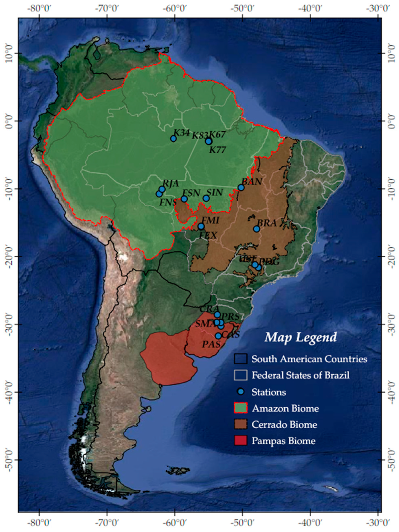
2.2. Study Region Description and Climatology

This study was performed over three major South American biomes: Amazon (AM), Cerrado (CE), and Pampa (PA). These biomes were selected based on their percentage of the continental coverage area, climatological impact in SA, and the availability of fluxes towers, as shown in Figure 1. The biomes with the EC towers correspond to 37.43% AM, 11.52% CE, and 4.77% PA of South America’s total area (17.8 mi km2).
The AM biome represents the tropical rainforest situated in the northern region of Brazil, south of Venezuela, center of Colombia, and Bolivia. The AM region consists mainly of dense leaf vegetation and evergreen trees. In this tropical forest, only 2–3% of direct solar radiation incident on top of trees reaches the surface [48]. The mean precipitation in the AM biome is near 270–280 mm month−1, and the lower precipitation rates are observed during the winter season [49]. The surface fluxes have a direct impact on the planetary boundary layer (PBL) height. In the Amazon region, the daily variability of PBL height during the drier months is strongly associated with the sensible heat flux [50]. During wetter months, PBL is mainly modulated by the latent heat flux and incident solar radiation. The release of latent heat flux supports diabatic heating, and consequently, water vapor condensation becomes an important mechanism of energy transport, which is strongly related to the dynamic of the tropical atmosphere [51], to better understand and continue assessing these patterns in the Amazon if of great relevance, since in the past 40 years, a temperature increase between 0.6 and 0.7 °C is being observed [52].
Regarding the CE region, the average annual rainfall can reach just over 1500 mm and is concentrated in the summer season, when evapotranspiration measurements can reach 900 mm [38]. During the wet season, the summer (December to March), the mean monthly precipitation is near 250 mm. In this biome, latent heat flux variations are more strongly linked to precipitation, which occurs due to the influence of synoptic-scale atmospheric phenomena, such as the Bolivian high (BH), South Atlantic convergence zone (SACZ), intertropical convergence zone (ITCZ), and low-level jets (LLJ) and, the variation of the energy as a function of solar radiation incident on the surface [53]. The predominant climate in the region is seasonal tropical, where rainfall values in the winter are lower than 50 mm and are considered a dry period. The average annual EC temperature ranges from 22 to 23 °C, the highest measurements can reach over 40 °C during the summer, and lower temperature near 0 °C may be observed in the winter [54].
The Brazilian Pampa corresponds to the northern portion of the Rio de la Plata grassland region [55], also known as Uruguayan savanna ecoregion [56], and encompasses an area of 193,383 km2 [57]. In Brazil, the Pampa is located between latitudes 28° S and 34° S and longitudes 49° W and 58° W, occupying 63% of the Rio Grande do Sul State. The Brazilian Pampa has both subtropical and temperate climates, showing four well-characterized seasons. The average annual precipitation in the Pampa region is ranging from 1200 to 1600 mm [58] with an average temperature of 18 °C [4]. The landscape consists of a mosaic of grasslands, different types of shrublands, low forests, and gallery forests along rivers. Although many landscapes, especially when dominated by grassland, might appear simple and homogeneous at first glance, the Pampa harbor has a remarkable biodiversity [59].

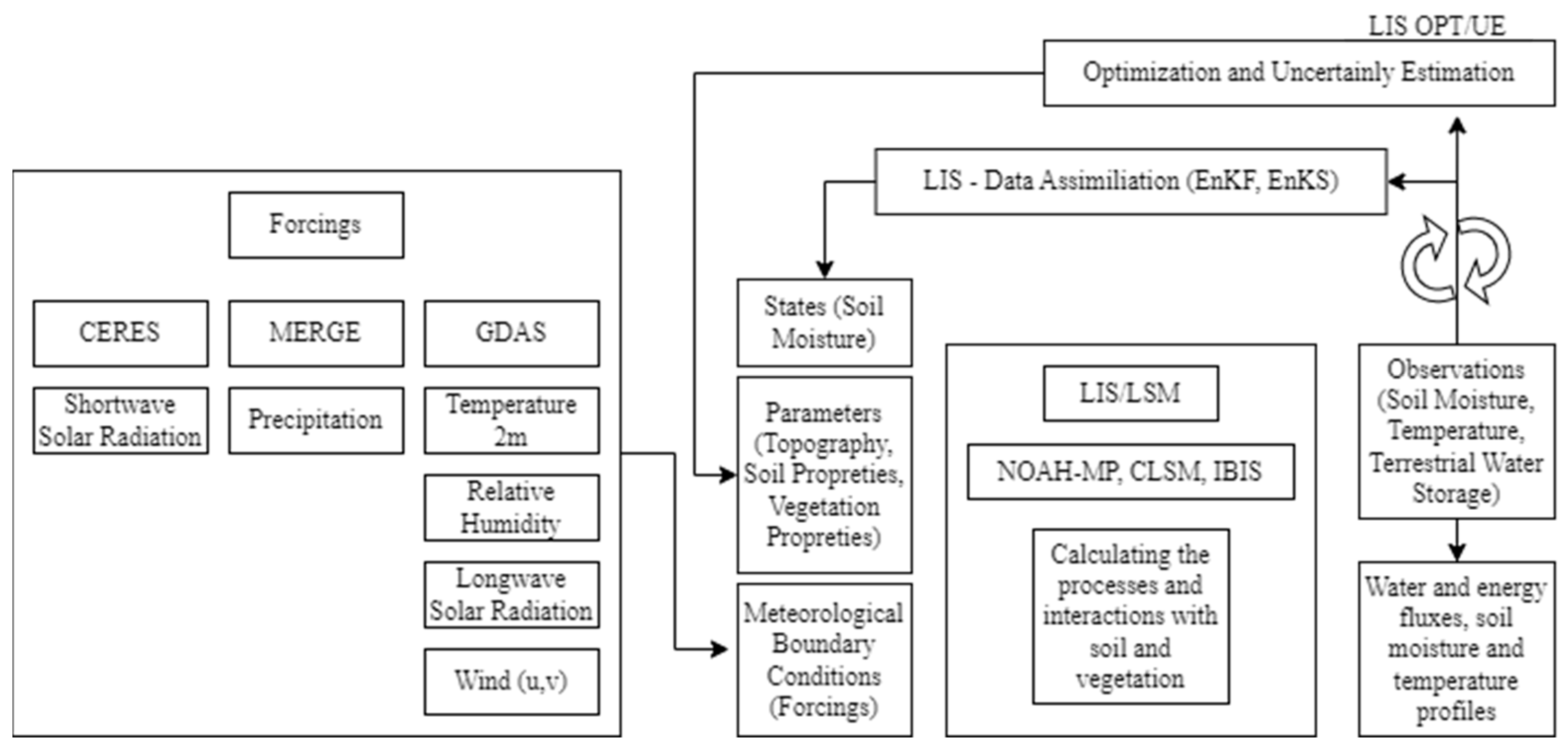
2.3. SALDAS-2 Description

The South America Land Data Assimilation System (SALDAS) is derived from the Land Data Assimilation System (LDAS). It was mainly developed to understand and determine the variables of energy and water balance focusing on the South American continent [9,60]. Currently, SALDAS has a 5 × 5 km resolution under the continental surface and a 3-h temporal resolution, and the atmospheric forcing comes from the Global Data Assimilation System (GDAS).
With the aim of using variables that are closer to observations, which can lead to an improvement in surface simulations of the models, we propose an enhancement of SALDAS (henceforth named South American Land Data Assimilation System Version 2 or SALDAS-2) as a way of contributing to the estimation of energy flows, in order to obtain a high-resolution data mesh for South America. Following the same methodology as Gonçalves et al. [24], this enhancement proposes the use of spatially distributed precipitation and downward shortwave radiation data over the South American continent. The forcings were introduced into the Land Information System (LIS), which is a framework used to more accurately describe topography, texture, soil transport, among other surface parameters. The LIS platform integrates observations and models, and through data assimilation, it allows the intercomparison of different surface models, as the boundary conditions in any given run remain the same [8,61].
The construction of SALDAS-2 was carried out using three of the models available in LIS: Noah-MP, CLSM, and IBIS. These models were chosen due to their great global use. Currently, the Noah-MP model is used as a boundary condition of the Global Forecast System [62], while the CLSM model can be used as one of the surface contour options on the regional WRF and the National Centers for Environmental Prediction (NCEP). IBIS is currently the surface model of the Brazilian Global Atmospheric Model (BAM) [63].
Current studies aim to use regional remote sensing products to acquire precipitation and radiation forcings, approaching observational measurements [64]. As a difference, SALDAS uses as forcing variables precipitation, shortwave radiation, longwave radiation, air temperature (2 m), specific humidity, surface pressure, and u and v wind components from GDAS [24]. In this version, the models used by SALDAS-2 (Noah-MP, CLSM, and IBIS) were configured with a resolution of 5 km under the South American domain (80° E at 31° W and 56° S at 12° N), likely SALDAS. The time period ranges from 2000 to 2020, with a temporal resolution of 3 h, daily and monthly outputs. For model runs, a 5-year spin-up was performed, as suggested by Kalnay and Yang [65]. This model configuration proposes a modification that involves incorporating spatially distributed data on precipitation and downward shortwave radiation that was used from Multi-Source Weighted-Ensemble Precipitation (MERGE) [66] and the Clouds and the Earth’s Radiant Energy System (CERES) [67], respectively. The other forcing variables of the models, longwave radiation, pressure, air temperature (2 m), specific humidity (2 m), and wind u and v components, were used from the Global Data Assimilation System (GDAS) [68]. Figure 2 summarizes the inputs used during the construction of SALDAS-2. For all these runs, the models consider a 2-m soil profile divided into four layers, 0–10, 10–40, 40–100, and 100–200 cm of depth.

2.3.1. Models and Configurations

The Noah-MP model incorporates various biological and physicochemical processes to improve surface flux estimates. It consists of 42 user-defined parameters, 30 of which are related to vegetation and 12 to soil. These parameters are divided into three layers of snow and four layers of soil depth. The Noah-MP model has the ability to compute surface temperature and estimate the energy balance of shortwave and longwave radiation, latent and sensible heat fluxes, and ground heat storage. The model includes dynamic vegetation and groundwater processes [69], and to do so, it parameterizes vegetation processes, stomatal resistance, US factor, runoff, surface drag coefficient, super frozen liquid water, frozen soil permeability, snow albedo, frozen/liquid partition, and radiative transfer [70].
In SALDAS-2, in addition to Noah-MP, the CLSM-Fortuna 2.5 model was incorporated, which is employed by NASA GEOS-5 for surface boundary parameterization in atmospheric modeling coupling [71]. The CLSM model is characterized by a soil temperature, with a depth range of 0 to 100 cm [72]. The soil moisture variable is not explicit; therefore, an equilibrium profile extending from the surface to the water table needs to be determined. To establish such a profile, the contribution of the surface balance zone (0–2 cm) and the root zone (0–100 cm) discretized by the model is required. Additionally, the snow cover parameterization of the model presents three layers considering phenomena such as melting, freezing, and changes in snow density [73].
The third model utilized in SALDAS-2 is the Integrated Biosphere Simulator (IBIS) [74], which is presently one of the models employed in the Brazilian Atmospheric Model (BAM), a general circulation model of the atmosphere (GCMA) developed by CPTEC/INPE (Centro de Previsão de Tempo e Estudos Climáticos/Instituto Nacional de Pesquisas Espaciais). IBIS has the largest number of below-ground layers among the three SALDAS-2 models, with 12 depth levels used to better parameterize the root system [75]. IBIS is a surface model that represents surface processes, such as environmental physics, canopy physiological processes, plant phenology, energy fluxes, carbon, and nutrient cycles. The model also features dynamic vegetation, similar to Noah-MP, including undergrowth and the tallest trees [74,76]. IBIS includes three layers describing snow cover and a module responsible for soil carbon stock and changes in vegetation on a timescale of months to years.
As previously mentioned, the LIS platform requires certain variables, known as forcings. This work divides the forcings into two categories. The first ones are derived from observation-based atmospheric data that are the closest to the regions of interest, such as radiation and precipitation (CERES and MERGE). The second set includes those derived from modeling-based atmospheric data, such as other forcings that originate from NCEP/GDAS.

2.3.2. Observation-Based Atmospheric Forcing

Radiation forcing—CERES: The observation-based shortwave radiation forcing used in SALDAS-2 was obtained from the Clouds and the Earth’s Radiant Energy System. CERES has a goal of developing ideal energy balance datasets and clouds using the Aqua and Terra satellites as bases for observations [77]. CERES prescribes height, thickness, particle size, cloud phase, and other cloud properties through the satellite observations, using the Earth Observation System (EOS), Joint Polar Satellite System (JPSS), Moderate Resolution Imaging Spectroradiometer (MODIS) and Visible Infrared Imaging Radiometer Suite (VIIRS) [77]. CERES data are available at: https://ceres.larc.nasa.gov/data/ accessed on 5 April 2023, and the product used was “SYN1deg”.
Precipitation forcing—MERGE: Similar to downward radiation, the precipitation data used by SALDAS-2 is also observation based. MERGE is derived from a merge of rain gauge estimation and satellite-based information. The result combines precipitation from observational data from the Global Telecommunication System (GTS), automated stations, and remote sensing precipitation derived from the Tropical Rainfall Measuring Mission (TRMM), Tropical Multisatellite Precipitation Analysis (TMPA), and Global Precipitation Measurement (GPM) [66]. MERGE data are available monthly over South America (90° W to 26° W, 57° S to 13° N) and daily over the Brazilian territory (75° W to 34° W, 35° S to 06° N) at a 5 km spatial resolution [66]. The MERGE data are initially provided as a quick estimate (called Early) and later as a more accurate estimate that includes more data (called Late). However, the in situ precipitation measurement network in South America is limited, which poses a challenge in obtaining accurate precipitation data. In such circumstances, the use of a MERGE product is beneficial as it helps mitigate the issue of sparse observational data, thereby reducing interpolation errors between the available measurement stations [78].

2.4. Reference Modelling Data

GDAS is a numerical data assimilation system developed by the National Oceanic and Atmospheric Administration (NOAA) that assimilates a wide range of observed atmospheric data to generate global analyses of the state of the atmosphere on a global scale (90° S to 90° N and 180° E to 180° W) and for the synoptic times (0000, 0006, 0012, 0018), which are available daily since January 2001 to the present [79]. These analyses are then used as operational initial conditions for the Global Forecast System (GFS) model. The system incorporates data from a variety of sources, including satellites, radiosondes, and surface observations, and then produces forecasts for up to 10 days in advance. The GDAS analyses support a wide range of applications, including weather forecasting, climate monitoring, and atmospheric research.
As a reference of global surface modeling, GLDAS is a system that uses advanced surface data assimilation techniques to generate information on the current state of surface fields [9]. The system integrates a large database of observation and model-derived base forcing with a spatial resolution of 0.25°. GLDAS is available at https://ldas.gsfc.nasa.gov/gldas, accessed on 5 April 2023. The necessary forcing variables, including air temperature and humidity, wind, surface pressure, and longwave radiation, are obtained from GDAS, as described previously. The radiative fluxes are derived from the Air Force Weather Agency’s (AFWA) Agricultural Meteorology modeling system (AGRMET), while precipitation is obtained from the near-real-time satellite-derived data from the U.S. Naval Research Laboratory (NRL).

2.5. Statistical Methods

To evaluate the performance of SALDAS-2 compared with GLDAS in relation to the flux towers, the normalized contribution information (NIC) was used. In this paper, model outputs were compared with the EC observations in terms of the RMSE, MBE, and r2.
The RMSE and MBE analyses were conducted to assess the contribution of radiation and precipitation forcing variables in the mean estimates of the EC towers in each of the studied biomes. The aim of this analysis is to identify the errors associated with the variables used by each of the SALDAS-2 and GLDAS models.
The RMSE denotes how errors related to observations and modeling are distributed; thus it is possible to observe how close the simulation is from the observations [80]. The RMSE is obtained based on Equation (4) below:
R M S E = ( P O ) 2 n
where O is the observational values, P is the simulations, and n is the number of samples.
The mean bias error (MBE), presented in Equation (5), aims to better understand the simulations’ tendency to underestimate (if MBE < 0) or overestimate (if MBE > 0) the EC values [80].
M B E = 1 n ( P O )
To compose the NIC evaluation, we also used the determination coefficient (r2) statistical method (Equation (6)), which represents the dependence between the sample and the observations. When r2 values are lower, the dependency is not expected. Therefore, higher r2 values indicate that the simulation is closer to observations [80];
r 2 = i = 1 n ( P P ) ( O O ) 2 i = n ( P P ) 2 i = n ( O O ) 2
where P′ is the mean of the simulations and O′ is the mean of the observations.
Aiming to analyze which SALDAS-2 models outperformed GLDAS for each EC tower over the SA biomes, the RMSE and r2 were used to calculate the NIC, denominated R M S E n i c , and R n i c . The models with lower errors indicate those that better represent the observations [81]. R M S E n i c is derived from Equation (7), and R n i c from Equation (8) below [82]:
R M S E n i c = R M S E O L R M S E D A R M S E O L
R M S E O L represents the RMSE from SALDAS-2 models and the observation, and R M S E D A is the RMSE between GLDAS and the observations.
Similarly, to analyze the contribution of the models in terms of their correlation with the observations, R n i c was used, according to the equation below:
R n i c = r 2 D A r 2 O L 1 r 2 O L
Broadly, we compared all the models with each other. Hereafter, SALDAS-2 run using the Noah model will be referred as SN, SALDAS-2 with CLSM as SC, SALDAS-2 with IBIS as SI, and SALDAS-2 with the Ensemble as SE. A similar approach was used for GLDAS models, however, only for GLDAS-Noah (GN) and GLDAS-CLSM (GC).

3. Results and Discussion

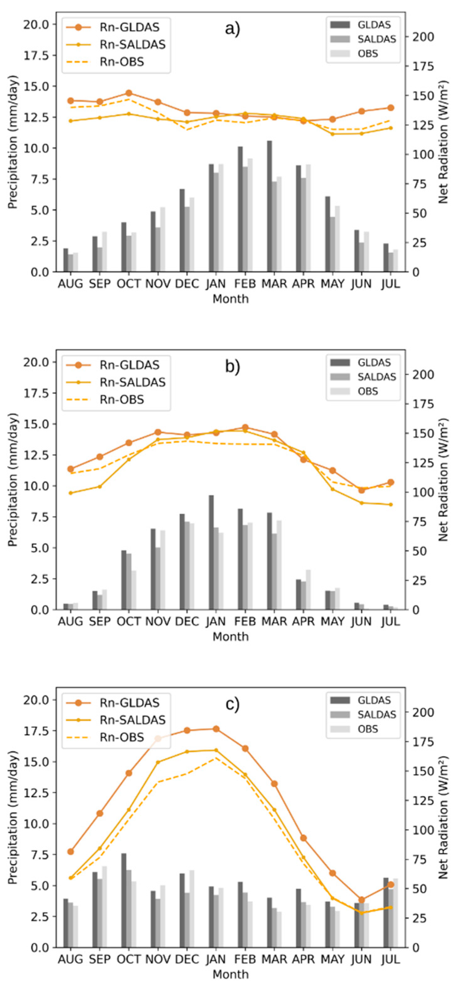
3.1. Precipitation and Radiation Forcings
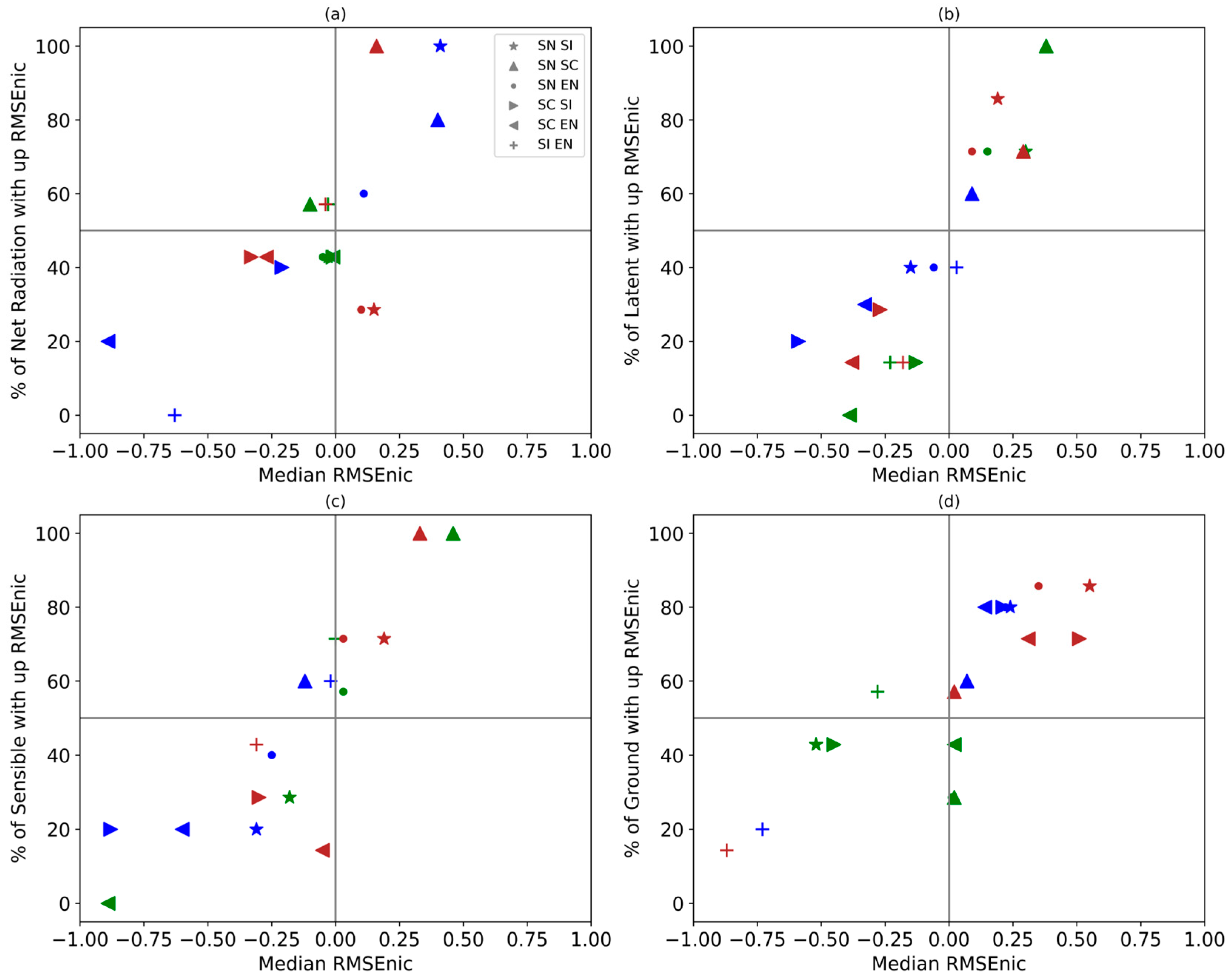
In the Amazon biome, the net radiation values obtained from CERES exhibit a closer agreement with the observations during the summer and early winter months, whereas GLDAS provides better results in the months of August to October. MERGE precipitation estimates tend to be superior to those used by GLDAS in most months of the year, as shown in Figure 3a and Table 2.
The variability of net radiation and precipitation in the Cerrado biome is represented by the forcings of SALDAS-2 and GLDAS (Figure 3b). During the transition months from winter to summer (September, October, and November), GLDAS tends to overestimate the net radiation by 5 W m−2, while SALDAS-2 presents an underestimate of about 10 W m−2 from May to November. In the summer months (December to February), both products yield values closer to the observations. With respect to precipitation, SALDAS-2 agrees more closely with the observations mainly during the summer months. Rozante et al. [83] report that good MERGE estimates are observed for Brazil during the summer months. The shortwave radiation used in SALDAS-2 tends to be lower than those observed at EC towers by ~15 W m−2 monthly. As demonstrated by Duveiller et al. [84], changes in vegetation cover alter the radiative and nonradiative properties of the surface, affecting the accuracy of CERES shortwave radiation estimates over biomes similar to the Cerrado.
In the Pampa biome, net radiation values obtained from CERES are closer to the in situ measurements compared with GLDAS throughout the year (Figure 3c). Moreira et al. [28] state that the remote sensing product performs well in representing the radiation over that region. Generally, SALDAS-2 and GLDAS exhibit oscillations, where, in the winter months, the models show values closer to the observations by around 1 mm month−1. However, in the transition months and summer, there is a significant difference of about 2.5 mm month−1 between the observed and modeled forcing, as shown in Figure 3c. It is noteworthy that the precipitation estimates obtained from SALDAS-2 tend to be closer to the tower observations in all biomes compared with GLDAS, and both forcings provide satisfactory representation of the seasonality in each region.
In general, it was observed that the SALDAS-2 precipitation presents the most favorable MBE results in all biomes, except for the Amazon (Table 2), where the MBE values for GLDAS precipitation showed an improvement of 0.21 mm month−1. These findings suggest that precipitation estimates derived solely from remote sensing may lead to errors in the Amazon region, given its cloudy conditions. SALDAS-2 tends to underestimate the net radiation for the region, while GLDAS overestimates it by about 7.07 W m−2. The Cerrado presented the smallest precipitation errors for the SALDAS-2 forcing when compared with the observed data. It should also be noted that in situations where the GLDAS precipitation is better than the SALDAS-2 precipitation in terms of MBE, the differences between the two are less than 1.3 mm month−1. In the Pampa biome, the GLDAS forcing tends to overestimate solar radiation, showing a bigger error than that of SALDAS-2. Furthermore, in the Pampa biome, CERES performs better than the AFWA radiation product in both RMSE and MBE indicators. The same is observed in terms of MERGE precipitation in relation to GPCP (Global Precipitation Climatology Project); the good performance of the products has already been demonstrated by [28,83].

3.2. SALDAS-2 Model

First, to assess the performance of SALDAS-2, an intercomparison of energy balance variables was conducted between all SALDAS-2 models (SN, SC, SI, and EN) for the Amazon, Cerrado, and Pampa biomes. Figure 4 depicts a scatterplot showing the normalized root mean square error values of energy balance ( R M S E n i c ) plotted against the percentage of flux towers that exhibited improved median errors or not for each model comparison. The figure compares the median errors from the reference model (model on the right in the legend) with the average errors from a second model (model on the left in the legend). The models were compared in pairs, and the icons with negative values on the X-axis indicate that the model on the left in the legend has greater relative errors than the model on the right in the legend. When comparing models with similar error averages, the median R M S E n i c is close to zero. Conversely, the relationship between models was observed to have higher differences in errors when the values were located closer to the extremes of the graph in relation to the X-axis. In Figure 4, it is also possible to notice that the icon located in the upper-right quadrant represents a measure of greater median errors by the model on the right in the legend. The average errors of this model were more significant when analyzing a higher percentage of towers. The opposite was observed for the icons located in the lower-left quadrant.
Figure 4 shows a comparison between the SALDAS-2 models for R M S E n i c , and Figure 5 represents a comparison for R n i c . The icons in both figures refer to the models being compared with each other; for example, the star icon represents a comparison between the SN and SI models, and the triangle icon represents a comparison between the SN and SC models, and so on. For the Amazon biome, the SN model stands out from the others in the measurements of latent and sensible heat flux. It also obtained lower average error values and showed improvement in a large number of towers (Figure 4b,c). The SC model is capable of representing the net radiation in the Amazon area similar to the SI and EN models. However, it has the worst performance when compared with the CE and PA biomes. Despite this, the SC model performs well in representing net radiation in the AM biome. This is due to the fact that the shortwave radiation in the model comes from CERES, which, according to Nascimento et al. [85], has less than 10% errors in relation to observations and more than 70% correlation for the region. Nonetheless, CLSM has difficulty in representing soil moisture and the amount of water that would be needed to saturate the soil in tropical forest regions [86]. Additionally, a study by Maertens et al. [87] found that the performance of the CLSM model was reasonable in describing surface variables, but inferior to other models tested, such as Noah-MP, in terms of simulating surface water fluxes and soil moisture. The authors highlighted that the inappropriate choice of soil and vegetation parameters, including soil water content and hydraulic conductivity, may have affected the model’s performance. Similarly, issues may have arisen with SALDAS-2, which, although improved precipitation estimates from MERGE, may still require careful consideration of vegetation parameters.
In the AM biome, the SN and SC models stand out for the obtained lower errors compared with the others, with the error being lower for a higher number of towers compared with SI and EN. Meanwhile, in the CE biome, there is a greater distribution of net radiation errors among the models. Specifically, the SC model presents larger errors in about 45% of the towers when compared with SI and EN models, which is the opposite of what happened in the AM biome. However, when compared with the SN model, the SC model shows higher average errors in 100% of the biome towers. The SN model also shows lower average errors in relation to SI and EN models. However, the improvement was distributed among a smaller number of towers, approximately 30%. For the Pampa biome, the SN model provides better results when compared with all the other models (SC, SI, and EN). Most of the towers showed better results, especially in comparison with the SI model (100% of the towers) and the SC model (80%).
The SC model is capable of representing the net radiation in the Amazon near SI and EN, but it has the worst performance when compared with the CE and PA biomes. The good performance of SC in representing the net radiation in the Amazon may be due to the fact that the shortwave radiation in the model comes from CERES, in which, according to Nascimento et al. [85], there are less than 10% errors in relation to observations and more than 70% correlation for the region. However, CLSM has difficulty in representing soil moisture and the amount of water that would be needed to saturate the soil in tropical forest regions [86].
In Figure 4a, it can be seen that for the Amazon biome (green icons), the SN model has errors close to 0 in net radiation in relation to EN and SI. In about 60% of the towers, the SN model had lower median errors. The same is valid for SC, where the model presented results very close to its SI and EN pairs, and obtained smaller average errors in about 60% of the analyzed towers. Comparing SN and SC, it is possible to observe that SN had higher median errors in relation to SC, and about 40% of the analyzed towers in the biome had lower errors for the model.
In the Amazon biome, SN and SC stand out as being models that obtained lower errors compared with the others, since, when compared with SI and EN, the errors are lower for a higher number of towers. CERES uses cloud discriminations and provides greater forcing of shortwave radiation to assist the models. In contrast, the discrimination of net radiation by CLSM and NOAH as well as IBIS is dependent on albedo and vegetation parameters, and is independent of water fluxes [72].
In the Cerrado, there is a greater distribution of net radiation errors among the models. SC shows larger errors in about 45% of the towers when compared with SI and EN, which is the opposite of what happened in the Amazon biome. However, when compared with SN, SC presents higher average errors in 100% of the biome towers. The SN model also presents lower average errors in relation to SI and EN; however, the improvement was distributed in a smaller number of towers, about 30%. For the Pampa, the SN model presents better results when compared with all the other models (SC, SI, and EN), where in most of the towers, the model presented better results, highlighting the comparison with SI (100% of the towers) and SC (80%).
When the simulations of latent heat flux were observed, SC is the model that performs worse than the SI and EN models in all studied biomes in a large percentage of towers. There is a difficulty for CLSM in solving latent heat flux over tropical forest regions, where the model has a tendency to overestimate [88]. According to Lei et al. [89], the CLSM evapotranspiration is the one with the greatest errors in the annual average under several regions of China, because the model tends to overestimate evapotranspiration in humid regions. Other authors have also shown that the use of CLSM can increase inherent errors in evapotranspiration estimates. Xia et al. [90] studied water storage estimates over regions of the United States of America and demonstrated that the model uses the leaf area index (LAI) to represent vegetation and estimate evapotranspiration processes. During the summer, in regions of open and heterogeneous vegetation, the model may tend to overestimate evapotranspiration.
It Is possible to observe that SN presents smaller errors than the other models of SALDAS-2, and when compared with SC, these smaller average errors were observed in 100% of the flux towers. Compared with SI and EN, Noah showed improvement in about 70% of the towers. The result below SN obtained by EN, in this case, is directly influenced by the overestimations from SC. The SN model is also better than the others in the Cerrado and in the Pampa when compared with SC (Figure 4b). Similar to Xia et al. [90], the Noah-MP model performed better in regions with a temperate climate, while arid and semiarid regions presented more challenges for simulating terrestrial water storage components.
In the sensible heat flux, the SN model also has smaller errors than SC (in 100% of the towers) and EN (in 60%) in the Amazon. Higher errors are observed by SN in 70% of the towers when compared with SI, which makes the errors between SN and EN very close to 0. The results corroborate an analyses by Li et al. [91], who evaluated NOAH-MP for different regions of the globe and demonstrated that the model tends to produce good results for fluxes in regions with dense vegetation cover, such as tropical forests.
In addition, for the Pampa biome, net radiation is better represented by SN compared with the others (Figure 4a). The good Noah-MP performance in the Amazon was demonstrated by Brunsnell et al. [92], where the Noah-MP model is more sensitive in representing ET in broadleaf forest regions than the MOD17A2 and MOD16A2 products. However, for the grassland and open shrubland regions, Noah has less accurate results than MODIS. Regarding tropical forests, Noah-MP performs well in representing surface moisture, and according to Bohm et al. [93], there is a slight tendency to overestimate the amount of latent heat flux and underestimate the sensible heat flux in grassland and forest regions.
In the Cerrado, the SN model also has the lowest mean errors, while SC has the highest mean error values when compared with all other models. However, for the Pampa, SN presents worse results when compared with the other models, but the average errors were distributed in 60%, 40%, and 20% of the towers in relation to SC, EN, and SI, respectively. According to Zhang et al. [10], Noah-MP tends to overestimate evapotranspiration during the summer period and underestimate other surface models in grassland and needleleaf regions.
The models exhibit diversity in the representation of the heat flux in the soil. For the Amazon, the SI model outperforms the others with better values of R M S E n i c observed in about 50% of the towers on average. SC is very close to SN and EN in most of the biomes’ flux towers. However, in the Pampa and Cerrado biomes, the SC and SN models fare better than SI in representing the stored heat flux. SN is better than all other models in both biomes, with errors smaller than 50% in several towers.
According to R n i c , the SN model has the best correlation values for net radiation observed in the Pampa biome, in more than 70% of the towers, compared with the other models. In the Amazon and Cerrado, the models have very close correlations with each other. In the Amazon, SN is better than SI and SC in 55% of the towers, but it is worse than the Ensemble in 70% of them. In the Cerrado, there is a variation in the number of towers in which each model presents better performance compared with the other (Figure 5a). It was observed that the average correlation between the models is higher for the other components of the energy balance than for net radiation. For the latent heat flux, SN has a better index than SC in 100% of the towers located in AM, and in approximately 70% of the towers, the model is better than SI and EN.
In the Cerrado biome, SN performs better than SI and EN, and they have average R n i c values close to 0 when compared with SC. However, in the Pampa biome, there are greater variations, and while SN performs better than SC, it presents worse results compared with SI and EN. The good performance of IBIS in PA is directly related to its ability to describe the processes of evapotranspiration and exchanges between roots and soil in more detail than SN. This is particularly relevant since three out of the five towers in the biome are located over flooded regions [94]. There are differences between Noah and IBIS that weigh when estimating latent heat flux; among them is the description of the phenology. IBIS describes with greater parameters and detail the stomatal resistance [94]. IBIS also has greater depth levels than the other models. The good performance of IBIS makes EN better than SN in the same number of towers.
SN has the sensible heat flux better represented than SC in all towers in the Amazon and Cerrado biomes, and it is also better than SI and EN in 70% of the Cerrado towers. Additionally, it is approximately 60% better than EN in the Amazon biome. SC is better than SN in 40% of the towers in the Pampa biome.

3.3. The Performance of SALDAS-2 in Relation to GLDAS

In this section, we compare SALDAS-2 surface models with GLDAS references in terms of their performance (Figure 6 and Figure 7). Generally, SALDAS-2 models show better performance than GLDAS models when simulating energy balance variables, with SN performing the best. For net radiation, EN generally has lower errors than GLDAS references, with SN being better than GN in approximately 71.43% of the flux towers in the Amazon region. However, in some flux towers, SN errors are significantly large, leading to a negative mean error. Similar observations are seen when comparing SI versus GN and EN versus GN models. According to Bohm et al. [93], the Noah-MP model presents errors in the estimation of energy fluxes due to failures in the parametrization of vegetation or soil, which can impact the hydrological distribution simulated by the model. Another factor to be considered is the input data of the model, which can also impact the estimation errors. The positive performance of Noah-MP in SALDAS-2 compared with GLDAS in the region may be because the South American model uses the regional precipitation from CPTEC/MERGE as input forcing, which makes the water availability closer to reality [87,90].
The use of regional forcings significantly improves the performance of SC in terms of net radiation in the AM biome, where it performs better than GN in approximately 71.43% of the flux towers and approximately 60% when compared with GC. Observations in the Amazon rainforest presented results opposite to those found by Jung et al. [95] in their research. The authors emphasized that uncertainties in simulating evapotranspiration (ET) are higher for the CLSM model than for the Noah model in forested regions in West Africa. However, the results obtained by the SALDAS model may be related to the use of precipitation and radiation forcing that are more suitable for the Amazon rainforest region, resulting in better flow estimates in this region.
In terms of latent heat flux, the pattern of SN errors compared with GN was observed in the Amazon and Pampa biomes, with SN having negative R M S E n i c values, indicating that its errors are greater than the reference. However, it performs better in most flux towers, and in those where it performs worse, it presents much larger average errors. In the Cerrado, the R M S E n i c values of SN and GN are very close in about 50% of the towers. EN outperforms GN in all biomes for latent heat flux, with SALDAS-2 showing improvements of approximately 55% in the Cerrado, 75% in the Amazon, and 100% in the Pampa, when compared with GC. GC has large errors when trying to represent the latent heat flux in all biomes.
According to Zhang et al. [10], CLSM tends to overestimate ET values in forest regions and has the ability to maintain average errors close to observation in grassland regions. This overestimation was also observed in our study, with the model having a tendency to overestimate the data observed by the towers in the winter months. However, in the summer, these overestimates are reduced, and the latent heat flux curve tends to stay close to the observation. These errors are reflected in sensible heat flux due to the model’s compensation for closing the energy balance. SALDAS-2 models have worse performance in the Amazon biome and better in the Cerrado and Pampa. Using the CLSM model with forcing variables closer to the observations resulted in a reduction of latent heat flux overestimation, leading to an improvement in the model (Figure 6b).
It is possible to notice that the SALDAS-2 models can be realistic for the seasonality of the net radiation during all the months of the year. However, SALDAS-2 simulations for net radiation over the Amazon biome have worse correlation than GLDAS in 80% of tower fluxes. This may be due to differences in the predominant vegetation in the 5x5 pixel, leading to errors in the estimates of net radiation over the region. In this case, EN simulations are better than the individual use of each model (SN, SC, and SI), reducing the number of towers where the models perform worse from 80% to about 55%. The SALDAS-2 models exhibit superior capabilities in estimating net radiation in both the Cerrado and Pampa biomes. Specifically, in the Cerrado, the SN model outperforms the GN model in 80% of the towers examined, while in the Pampa biome, the SN model displays superior correlation estimates in all of the towers examined, surpassing both GN and GC models.
In the case of evaluating heat fluxes, there is a significant difference between the GLDAS and SALDAS-2 models in the Pampa biome. For the latent heat flux, the SN model exhibits a stronger correlation in the Amazon biome, with over 80% of towers displaying superior estimates. However, the SN model encounters difficulties in representing the latent heat flux in the Pampa biome. This can be attributed to the location of the flux towers in heterogeneous land cover regions in the southern region, which complicates accurate modeling estimates.
The GLDAS models demonstrate greater correlations in both sensible and ground heat fluxes across all biomes. This indicates that the low resolution of the models does not necessarily improve the correlation of sensitive and latent fluxes.
Models that fail to adequately represent the characteristics of land cover at a given tower location struggle to capture the seasonality of latent and sensible heat fluxes. The SC model, in particular, has difficulty achieving good correlations with observed data due to discrepancies in surface coverage as represented by the towers and GLDAS. This issue is particularly pronounced in the Cerrado and Pampa biomes, where heterogeneity is more significant. In contrast, the sensible heat flux tends to compensate for any overloading in the latent heat flux, as the model seeks to close the energy balance by accounting for energy gains or losses.
It is possible to notice that the SALDAS-2 models can be realistic for the seasonality of the net radiation during all the months of the year. The simulations from SALDAS-2 for net radiation over the Amazon biome have a worse correlation than GLDAS in 80% of flux towers. In almost all towers of the Amazon biome, the land cover is similar in both surface models (SALDAS-2 and GLDAS). However, in the SN and SC models, in most towers, the predominant vegetation in the 5 × 5 pixel is different from that described by GLDAS, which can lead to errors in the estimates of net radiation over the region [96]. In this case, the EN simulations are better than the individual use of each model (SN, SC, and SI), where the number of towers in which the models were worse was reduced from 80% to about 55%. The SALDAS-2 models are greater at estimating net radiation in the Cerrado and Pampa. In the Cerrado, the SN model outperforms the GN model in 80% of the flux towers, while in the Pampa biome, the same model displays superior correlation estimates in all of the towers examined, surpassing both GN and GC models.
There is a significant difference between GLDAS and SALDAS-2 models in the PA biome when evaluating heat fluxes. The SN model exhibits a stronger correlation for latent heat flux in the AM biome, with over 80% of towers displaying superior estimates. However, the SN model encounters difficulties in representing the latent heat flux in the PA biome (Figure 7b). This can be attributed to the location of flux towers in heterogeneous land cover regions in the southern region, which complicates accurate modeling estimates. The average flux is affected by adjacent fields, making correct tilling difficult [70]. The GLDAS models show greater correlations on sensible and ground heat fluxes in all biomes, indicating that a low resolution of the models does not necessarily improve the correlation of sensitive and latent fluxes.
Individually, the models whose representation of the land cover is not equal to the characteristics of the tower at the point have greater difficulty in representing the seasonality of latent and sensible heat fluxes. The SC has extreme difficulty in obtaining good correlations with the observed data because, in general, the surface coverage is different from that represented by the towers and GLDAS. This causes the model to perform poorly in the Cerrado and Pampa, where heterogeneity is greater. The opposite is observed in the sensible heat flux since, for the purpose of compensation to close the energy balance, any overload in the latent heat flux is reflected in the sensible one, as the model tends to compensate for energy gains or losses.

3.4. Limitations and Uncertainties of the SALDAS-2 Models

Although SN yielded satisfactory results in simulating the energy balance variables, it exhibits weaknesses in characterizing vegetation, which may lead to an inadequate representation of the vegetation dynamics across different regions. Moreover, the accuracy of precipitation data may vary by region, thereby affecting the hydrological simulations and water processes. Furthermore, the model tends to exhibit errors in estimating the latent and sensible heat fluxes in the PA biome, possibly due to difficulties in simulating vegetation dynamics, as the surface cover in the region displays heterogeneous characteristics.
A study by Cuntz et al. [97] compared various parameter sets of the Noah-MP model, and the authors describe that for better estimations of Noah-MP, it is crucial to conduct calibration to improve the accuracy of hydrological simulations. Moreover, Noah-MP exhibited problems in estimating ET and surface runoff under different surface conditions. These errors were possibly attributed to imprecision in the parameters related to water transfer on the soil surface.
Although the SC model is widely used for simulating energy fluxes and ET, it presents limitations in representing vegetation dynamics in some regions. In particular, the model tends to overestimate latent heat flux and underestimate sensible heat flux over the CE biome. This can be explained by the fact that the Cerrado region is highly heterogeneous, with great variation in vegetation cover over time and space. The SC model may have difficulties in capturing this heterogeneity, resulting in imprecise estimates of energy fluxes. Additionally, the seasonality of the Cerrado, with well-defined dry and rainy periods, can also pose challenges for the model’s estimates.
It is quite plausible to assert that one of the main causes of errors in estimating energy fluxes by the model is associated with vegetation dynamics. This is because vegetation cover directly affects the LAI, which is an important variable for partitioning energy fluxes in the model. A study by Lei et al. [89] demonstrated that the transition between wet and dry climate regimes is characterized by large variability in soil moisture, which can impact the CLSM model. It exhibits a tendency to overestimate the coupling strength between soil moisture and latent heat in transitional climate regimes, such as in the Great Plains of North America, Central Asia, and Central Australia. Similarly, the model presents challenges in estimating energy fluxes over the CE biome.
While the SI model can be applied to various types of ecosystems, including tropical forests, it may have some specific limitations in this type of environment. Some of these difficulties may be associated with a low representation of canopy heterogeneity, which can lead to an underestimation of spatial variation in energy and water exchange. Another limitation is the difficulty in simulating evapotranspiration in hydromorphic soils, which are common in tropical forest areas. In addition, the representation of nutrient cycling in IBIS may not be as detailed as in other models, limiting the accuracy of the simulation in this aspect.
The performance of SI depends on the quality and accuracy of input parameters, and in forest ecosystems, there may be limitations in the availability of data to estimate these parameters, which can affect the accuracy of the simulation. It is important to note that these limitations do not invalidate the application of the IBIS model in tropical forests, but rather emphasize the need to evaluate the model’s performance and adjust it to ensure simulation accuracy.

4. Conclusions

This study demonstrates the promising potential of using regional variables to force surface models to obtain more realistic simulations. The use of remote sensing products, such as precipitation and shortwave radiation, proved effective in improving the accuracy of flux tower observations. The MERGE and CERES models provided good estimates of precipitation and shortwave radiation in much of South America, particularly in the northern and southeastern regions.
The SALDAS-2 model tends to overestimate evapotranspiration in these regions and, to compensate for the energy balance, underestimate sensible heat flux values to balance the net radiation, as the soil heat storage values are lower compared with other energy balance variables. This is because the soil heat storage values are lower compared with other energy balance variables. The use of remote sensing variables for radiation and precipitation resulted in better estimates of latent heat flux in forested areas in the CLSM model obtained by SALDAS-2. This outcome supports the aim of this study to improve energy balance variables using regional radiation and precipitation forcings.
However, the SALDAS-2 model performed best in grassland regions, as its low resolution provided a better representation of vegetation and surrounding advective flows, thus improving the estimates. For this region, RMSE values were reduced from 38.44 W m−2 for GC to 22.7 W m−2 for SC, while sensible heat was reduced from 17 W m−2 for GC to 10.41 W m−2 for SC.
In general, the Noah-MP and Ensemble models provided better results for flux estimates. However, using the EN model by SALDAS-2 improved the estimates of soil heat flux in all biomes when compared with individual GLDAS models and their average estimates. This is because when one SALDAS-2 model produces an error, the others tend to compensate for it.
Finally, while presenting an improved framework for SALDAS called SALDAS-2, with the aim of producing consistent land surface estimates for South America, this study highlights the potential of using regional variables derived from remote sensing products to improve the accuracy of surface models, especially in regions with heterogeneous land cover. The results show that the use of precipitation and shortwave radiation data from remote sensing products, coupled with the SALDAS-2 models, leads to better estimates of latent heat flux under forest regions. Moreover, the low resolution of SALDAS-2 models is beneficial for grassland regions due to their better representation of vegetation and advective fluxes. The use of Ensemble methods, such as EN, improves the estimation of ground heat flux across all biomes. The findings of this study can contribute to the improvement of regional and global climate models. Future studies should continue to explore the use of remote sensing products to better represent the complex energy balance in different regions.

Author Contributions

Á.V.A.d.Á. generated and analyzed the results. Á.V.A.d.Á. and L.G.G.d.G. wrote the manuscript. Á.V.A.d.Á. and V.d.A.S. organized the manuscript. L.G.G.d.G., V.d.A.S., D.R.R. and A.R. reviewed the manuscript. D.R.R., M.S.B. and N.G.M. conceived and designed the experiments in flux tower data. L.E.R.A., G.D.G., B.M.M. and A.G. supported in the applications of the models. L.G.G.d.G. supervised and advised all the research work that led to this paper. All authors have read and agreed to the published version of the manuscript.

Funding

The authors acknowledge the National Council for Scientific and Technological Development (CNPq–Brazil) and the Coordination for the Improvement of Higher Education Personnel (CAPES–Brazil, funding code 001) for their financial support.

Informed Consent Statement

Not applicable.

Data Availability Statement

Not applicable.

Acknowledgments

The authors acknowledge the INPE and the actual Brazilian government for their support of science, which allowed us to conduct this research and contribute to the advancement of knowledge in our field.

Conflicts of Interest

The authors declare no conflict of interest.

References

  1. Fisher, R.A.; Koven, C.D. Perspectives on the Future of Land Surface Models and the Challenges of Representing Complex Terrestrial Systems. J. Adv. Model. Earth Syst. 2020, 12, e2018MS001453. [Google Scholar] [CrossRef]
  2. Blyth, E.M.; Arora, V.K.; Clark, D.B.; Dadson, S.J.; De Kauwe, M.G.; Lawrence, D.M.; Melton, J.R.; Pongratz, J.; Turton, R.H.; Yoshimura, K.; et al. Advances in Land Surface Modelling. Curr. Clim. Chang. Reports 2021, 7, 45–71. [Google Scholar] [CrossRef]
  3. Glenn, E.P.; Huete, A.R.; Nagler, P.L.; Hirschboeck, K.K.; Brown, P. Integrating Remote Sensing and Ground Methods to Estimate Evapotranspiration. CRC. Crit. Rev. Plant Sci. 2007, 26, 139–168. [Google Scholar] [CrossRef]
  4. Pörtner, H.-O.; Roberts, D.C.; Tignor, M.; Poloczanska, E.S.; Mintenbeck, K.; Alegría, A.; Craig, M.; Langsdorf, S.; Löschke, S.; Möller, V.; et al. Climate Change 2022: Impacts, Adaptation, and Vulnerability; IPCC: Geneva, Switzerland, 2022.
  5. Save, H.; Bettadpur, S.; Tapley, B.D. High-Resolution CSR GRACE RL05 Mascons. J. Geophys. Res. Solid Earth 2016, 121, 7547–7569. [Google Scholar] [CrossRef]
  6. Libonati, R.; Pereira, J.M.C.; Da Camara, C.C.; Peres, L.F.; Oom, D.; Rodrigues, J.A.; Santos, F.L.M.; Trigo, R.M.; Gouveia, C.M.P.; Machado-Silva, F.; et al. Twenty-First Century Droughts Have Not Increasingly Exacerbated Fire Season Severity in the Brazilian Amazon. Sci. Rep. 2021, 11, 4400. [Google Scholar] [CrossRef]
  7. Rodell, M.; Famiglietti, J.S.; Wiese, D.N.; Reager, J.T.; Beaudoing, H.K.; Landerer, F.W.; Lo, M.-H. Emerging Trends in Global Freshwater Availability. Nature 2018, 557, 651–659. [Google Scholar] [CrossRef]
  8. Kumar, S.; Peterslidard, C.; Tian, Y.; Houser, P.; Geiger, J.; Olden, S.; Lighty, L.; Eastman, J.; Doty, B.; Dirmeyer, P. Land Information System: An Interoperable Framework for High Resolution Land Surface Modeling. Environ. Model. Softw. 2006, 21, 1402–1415. [Google Scholar] [CrossRef]
  9. Rodell, M.; Famiglietti, J.S.; Chen, J.; Seneviratne, S.I.; Viterbo, P.; Holl, S.; Wilson, C.R. Basin Scale Estimates of Evapotranspiration Using GRACE and Other Observations. Geophys. Res. Lett. 2004, 31, L20504. [Google Scholar] [CrossRef]
  10. Zhang, Z.; Barlage, M.; Chen, F.; Li, Y.; Helgason, W.; Xu, X.; Liu, X.; Li, Z. Joint Modeling of Crop and Irrigation in the Central United States Using the Noah-MP Land Surface Model. J. Adv. Model. Earth Syst. 2020, 12. [Google Scholar] [CrossRef]
  11. Meng, X.; Wang, H.; Wu, Y.; Long, A.; Wang, J.; Shi, C.; Ji, X. Investigating Spatiotemporal Changes of the Land-Surface Processes in Xinjiang Using High-Resolution CLM3.5 and CLDAS: Soil Temperature. Sci. Rep. 2017, 7, 13286. [Google Scholar] [CrossRef]
  12. Kumar, S.V.; Zaitchik, B.F.; Peters-Lidard, C.D.; Rodell, M.; Reichle, R.; Li, B.; Jasinski, M.; Mocko, D.; Getirana, A.; De Lannoy, G.; et al. Assimilation of Gridded GRACE Terrestrial Water Storage Estimates in the North American Land Data Assimilation System. J. Hydrometeorol. 2016, 17, 1951–1972. [Google Scholar] [CrossRef]
  13. Hazra, A.; McNally, A.; Slinski, K.; Arsenault, K.R.; Shukla, S.; Getirana, A.; Jacob, J.P.; Sarmiento, D.P.; Peters-Lidard, C.; Kumar, S.V.; et al. NASA’s NMME-Based S2S Hydrologic Forecast System for Food Insecurity Early Warning in Southern Africa. J. Hydrol. 2023, 617, 129005. [Google Scholar] [CrossRef]
  14. Getirana, A.; Rodell, M.; Kumar, S.; Beaudoing, H.K.; Arsenault, K.; Zaitchik, B.; Save, H.; Bettadpur, S. GRACE Improves Seasonal Groundwater Forecast Initialization over the United States. J. Hydrometeorol. 2020, 21, 59–71. [Google Scholar] [CrossRef]
  15. Jung, H.C.; Kang, D.-H.; Kim, E.; Getirana, A.; Yoon, Y.; Kumar, S.; Peters-lidard, C.D.; Hwang, E. Towards a Soil Moisture Drought Monitoring System for South Korea. J. Hydrol. 2020, 589, 125176. [Google Scholar] [CrossRef]
  16. Collischonn, W.; Allasia, D.; Da Silva, B.C.; Tucci, C.E.M. The MGB-IPH Model for Large-Scale Rainfall—Runoff Modelling. Hydrol. Sci. J. 2007, 52, 878–895. [Google Scholar] [CrossRef]
  17. Niu, G.-Y.; Yang, Z.-L.; Mitchell, K.E.; Chen, F.; Ek, M.B.; Barlage, M.; Kumar, A.; Manning, K.; Niyogi, D.; Rosero, E.; et al. The Community Noah Land Surface Model with Multiparameterization Options (Noah-MP): 1. Model Description and Evaluation with Local-Scale Measurements. J. Geophys. Res. 2011, 116, D12109. [Google Scholar] [CrossRef]
  18. Bechtold, M.; De Lannoy, G.J.M.; Koster, R.D.; Reichle, R.H.; Mahanama, S.P.; Bleuten, W.; Bourgault, M.A.; Brümmer, C.; Burdun, I.; Desai, A.R.; et al. PEAT-CLSM: A Specific Treatment of Peatland Hydrology in the NASA Catchment Land Surface Model. J. Adv. Model. Earth Syst. 2019, 11, 2130–2162. [Google Scholar] [CrossRef]
  19. Getirana, A.C.V.; Dutra, E.; Guimberteau, M.; Kam, J.; Li, H.-Y.; Decharme, B.; Zhang, Z.; Ducharne, A.; Boone, A.; Balsamo, G.; et al. Water Balance in the Amazon Basin from a Land Surface Model Ensemble. J. Hydrometeorol. 2014, 15, 2586–2614. [Google Scholar] [CrossRef]
  20. Getirana, A.; Kirschbaum, D.; Mandarino, F.; Ottoni, M.; Khan, S.; Arsenault, K. Potential of GPM IMERG Precipitation Estimates to Monitor Natural Disaster Triggers in Urban Areas: The Case of Rio de Janeiro, Brazil. Remote Sens. 2020, 12, 4095. [Google Scholar] [CrossRef]
  21. Kumar, S.; Getirana, A.; Libonati, R.; Hain, C.; Mahanama, S.; Andela, N. Changes in Land Use Enhance the Sensitivity of Tropical Ecosystems to Fire-Climate Extremes. Sci. Rep. 2022, 12, 964. [Google Scholar] [CrossRef] [PubMed]
  22. Davidson, E.A.; Artaxo, P. Globally Significant Changes in Biological Processes of the Amazon Basin: Results of the Large-Scale Biosphere-Atmosphere Experiment. Glob. Chang. Biol. 2004, 10, 519–529. [Google Scholar] [CrossRef]
  23. Keller, M.; Alencar, A.; Asner, G.P.; Braswell, B.; Bustamante, M.; Davidson, E.; Feldpausch, T.; Fernandes, E.; Goulden, M.; Kabat, P.; et al. Ecological Research in the Large-Scale Biosphere– Atmosphere Experiment in Amazonia: Early Results. Ecol. Appl. 2004, 14, 3–16. [Google Scholar] [CrossRef]
  24. Gonçalves, L.G.G.; Borak, J.S.; Costa, M.H.; Saleska, S.R.; Baker, I.; Restrepo-Coupe, N.; Muza, M.N.; Poulter, B.; Verbeeck, H.; Fisher, J.B.; et al. Overview of the Large-Scale Biosphere–Atmosphere Experiment in Amazonia Data Model Intercomparison Project (LBA-DMIP). Agric. For. Meteorol. 2013, 182–183, 111–127. [Google Scholar] [CrossRef]
  25. Keller, M.; Bustamante, M.; Gash, J.; Dias, P.S. Amazonia and Global Change; American Geophysical Union: Washington, DC, USA, 2009. [Google Scholar]
  26. Roberti, D.R.; Acevedo, O.C.; Moraes, O.L.L. A Brazilian Network of Carbon Flux Stations. Eos, Trans. Am. Geophys. Union 2012, 93, 203. [Google Scholar] [CrossRef]
  27. Davidson, E.A.; de Araújo, A.C.; Artaxo, P.; Balch, J.K.; Brown, I.F.; Bustamante, M.M.C.; Coe, M.T.; DeFries, R.S.; Keller, M.; Longo, M.; et al. The Amazon Basin in Transition. Nature 2012, 481, 321–328. [Google Scholar] [CrossRef] [PubMed]
  28. Moreira, A.A.; Ruhoff, A.L.; Roberti, D.R.; Souza, V.d.A.; da Rocha, H.R.; de Paiva, R.C.D. Assessment of Terrestrial Water Balance Using Remote Sensing Data in South America. J. Hydrol. 2019, 575, 131–147. [Google Scholar] [CrossRef]
  29. Von Randow, C.; Manzi, A.O.; Kruijt, B.; de Oliveira, P.J.; Zanchi, F.B.; Silva, R.L.; Hodnett, M.G.; Gash, J.H.C.; Elbers, J.A.; Waterloo, M.J.; et al. Comparative Measurements and Seasonal Variations in Energy and Carbon Exchange over Forest and Pasture in South West Amazonia. Theor. Appl. Climatol. 2004, 78, 5–26. [Google Scholar] [CrossRef]
  30. Araújo, A.C.; Nobre, A.D.; Kruijt, B.; Elbers, J.A.; Dallarosa, R.; Stefani, P.; Von Randow, C.; Manzi, A.O.; Culf, A.D.; Gash, H.C.; et al. Comparative Measurements of Carbon Dioxide Fluxes from Two Nearby Towers in a Central Amazonian Rainforest: The Manaus LBA Site. J. Geophys. Res. 2002, 107, 8090. [Google Scholar] [CrossRef]
  31. Saleska, S.R.; Miller, S.D.; Matross, D.M.; Goulden, M.L.; Wofsy, S.C.; da Rocha, H.R.; de Camargo, P.B.; Crill, P.; Daube, B.C.; de Freitas, H.C.; et al. Carbon in Amazon Forests: Unexpected Seasonal Fluxes and Disturbance-Induced Losses. Science 2003, 302, 1554–1557. [Google Scholar] [CrossRef] [PubMed]
  32. Sakai, R.K.; Fitzjarrald, D.R.; Moraes, O.L.L.; Staebler, R.M.; Acevedo, O.C.; Czikowsky, M.J.; da Silva, R.; Brait, E.; Miranda, V. Land-Use Change Effects on Local Energy, Water, and Carbon Balances in an Amazonian Agricultural Field. Glob. Chang. Biol. 2004, 10, 895–907. [Google Scholar] [CrossRef]
  33. Goulden, M.L.; Miller, S.D.; da Rocha, H.R.; Menton, M.C.; de Freitas, H.C.; e Silva Figueira, A.M.; de Sousa, C.A.D. Diel and Seasonal Patterns of Tropical Forest CO2 Exchange. Ecol. Appl. 2004, 14, 42–54. [Google Scholar] [CrossRef]
  34. Biudes, M.S.; Vourlitis, G.L.; Machado, N.G.; de Arruda, P.H.Z.; Neves, G.A.R.; de Almeida Lobo, F.; Neale, C.M.U.; de Souza Nogueira, J. Patterns of Energy Exchange for Tropical Ecosystems across a Climate Gradient in Mato Grosso, Brazil. Agric. For. Meteorol. 2015, 202, 112–124. [Google Scholar] [CrossRef]
  35. Borma, L.S.; da Rocha, H.R.; Cabral, O.M.; von Randow, C.; Collicchio, E.; Kurzatkowski, D.; Brugger, P.J.; Freitas, H.; Tannus, R.; Oliveira, L.; et al. Atmosphere and Hydrological Controls of the Evapotranspiration over a Floodplain Forest in the Bananal Island Region, Amazonia. J. Geophys. Res. 2009, 114, G01003. [Google Scholar] [CrossRef]
  36. Santos, A.J.B.; Silva, G.T.D.A.; Miranda, H.S.; Miranda, A.C.; Lloyd, J. Effects of Fire on Surface Carbon, Energy and Water Vapour Fluxes over Campo Sujo Savanna in Central Brazil. Funct. Ecol. 2003, 17, 711–719. [Google Scholar] [CrossRef]
  37. Hasler, N.; Avissar, R. What Controls Evapotranspiration in the Amazon Basin? J. Hydrometeorol. 2007, 8, 380–395. [Google Scholar] [CrossRef]
  38. Da Rocha, H.R.; Freitas, H.C.; Rosolem, R.; Juárez, R.I.N.; Tannus, R.N.; Ligo, M.A.; Cabral, O.M.R.; Dias, M.A.F.S. Measurements of CO2 Exchange over a Woodland Savanna (Cerrado Sensu Stricto) in Southeast Brasil. Biota Neotrop. 2002, 2, 1–11. [Google Scholar] [CrossRef]
  39. Cabral, O.M.R.; da Rocha, H.R.; Ligo, M.A.V.; Brunini, O.; Dias, M.A.F.S. Fluxos Turbulentos de Calor Sensível, Vapor de Água e CO2 Sobre Plantação de Cana-de-Açucar (Saccharum Sp.) Em Sertãozinho-SP. Rev. Bras. Meteorol. 2003, 18, 61–70. [Google Scholar]
  40. Souza, V.d.A.; Roberti, D.R.; Ruhoff, A.L.; Zimmer, T.; Adamatti, D.S.; de Gonçalves, L.G.G.; Diaz, M.B.; de Cássia Marques Alves, R.; de Moraes, O.L.L. Evaluation of MOD16 Algorithm over Irrigated Rice Paddy Using Flux Tower Measurements in Southern Brazil. Water 2019, 11, 1911. [Google Scholar] [CrossRef]
  41. Moreira, V.S.; Roberti, D.R.; Minella, J.P.; de Gonçalves, L.G.G.; Candido, L.A.; Fiorin, J.E.; Moraes, O.L.L.; Timm, A.U.; Carlesso, R.; Degrazia, G.A. Seasonality of Soil Water Exchange in the Soybean Growing Season in Southern Brazil. Sci. Agric. 2015, 72, 103–113. [Google Scholar] [CrossRef]
  42. Rubert, G.C.D.; Souza, V.d.A.; Zimmer, T.; Veeck, G.P.; Mergen, A.; Bremm, T.; Ruhoff, A.; de Gonçalves, L.G.G.; Roberti, D.R. Patterns and Controls of the Latent and Sensible Heat Fluxes in the Brazilian Pampa Biome. Atmosphere 2021, 13, 23. [Google Scholar] [CrossRef]
  43. Timm, A.U.; Roberti, D.R.; Streck, N.A.; de Gonçalves, L.G.G.; Acevedo, O.C.; Moraes, O.L.L.; Moreira, V.S.; Degrazia, G.A.; Ferlan, M.; Toll, D.L. Energy Partitioning and Evapotranspiration over a Rice Paddy in Southern Brazil. J. Hydrometeorol. 2014, 15, 1975–1988. [Google Scholar] [CrossRef]
  44. Rubert, G.C.; Roberti, D.R.; Pereira, L.S.; Quadros, F.L.F.; Velho, H.F.D.C.; Moraes, O.L.L.D. Evapotranspiration of the Brazilian Pampa Biome: Seasonality and Influential Factors. Water 2018, 10, 1864. [Google Scholar] [CrossRef]
  45. Alberto, M.C.R.; Wassmann, R.; Hirano, T.; Miyata, A.; Hatano, R.; Kumar, A.; Padre, A.; Amante, M. Comparisons of Energy Balance and Evapotranspiration between Flooded and Aerobic Rice Fields in the Philippines. Agric. Water Manag. 2011, 98, 1417–1430. [Google Scholar] [CrossRef]
  46. Diaz, M.B.; Roberti, D.R.; Carneiro, J.V.; Souza, V.d.A.; de Moraes, O.L.L. Dynamics of the Superficial Fluxes over a Flooded Rice Paddy in Southern Brazil. Agric. For. Meteorol. 2019, 276–277, 107650. [Google Scholar] [CrossRef]
  47. Twine, T.E.; Kustas, W.P.; Norman, J.M.; Cook, D.R.; Houser, P.R.; Meyers, T.P.; Prueger, J.H.; Wesley, M.L. Correcting Eddy Covariance Flux Underestimates over Grassland. Agric. For. Meteorol. 2000, 103, 279–300. [Google Scholar] [CrossRef]
  48. Huete, A.R.; Didan, K.; Shimabukuro, Y.E.; Ratana, P.; Saleska, S.R.; Hutyra, L.R.; Yang, W.; Nemani, R.R.; Myneni, R. Amazon Rainforests Green-up with Sunlight in Dry Season. Geophys. Res. Lett. 2006, 33, L06405. [Google Scholar] [CrossRef]
  49. Cavalcante, R.B.L.; da Silva Ferreira, D.B.; Pontes, P.R.M.; Tedeschi, R.G.; da Costa, C.P.W.; de Souza, E.B. Evaluation of Extreme Rainfall Indices from CHIRPS Precipitation Estimates over the Brazilian Amazonia. Atmos. Res. 2020, 238, 104879. [Google Scholar] [CrossRef]
  50. Henkes, A.; Fisch, G.; Machado, L.A.T.; Chaboureau, J.-P. Morning Boundary Layer Conditions for Shallow to Deep Convective Cloud Evolution during the Dry Season in the Central Amazon. Atmos. Chem. Phys. 2021, 21, 13207–13225. [Google Scholar] [CrossRef]
  51. Fisher, J.B.; Malhi, Y.; Bonal, D.; Da Rocha, H.R.; De Araújo, A.C.; Gamo, M.; Goulden, M.L.; Rano, T.H.; Huete, A.R.; Kondo, H.; et al. The Land-Atmosphere Water Flux in the Tropics. Glob. Chang. Biol. 2009, 15, 2694–2714. [Google Scholar] [CrossRef]
  52. Jiménez-Muñoz, J.C.; Mattar, C.; Barichivich, J.; Santamaría-Artigas, A.; Takahashi, K.; Malhi, Y.; Sobrino, J.A.; van der Schrier, G. Record-Breaking Warming and Extreme Drought in the Amazon Rainforest during the Course of El Niño 2015–2016. Sci. Rep. 2016, 6, 33130. [Google Scholar] [CrossRef] [PubMed]
  53. Reboita, M.S.; Ambrizzi, T.; Silva, B.A.; Pinheiro, R.F.; da Rocha, R.P. The South Atlantic Subtropical Anticyclone: Present and Future Climate. Front. Earth Sci. 2019, 7. [Google Scholar] [CrossRef]
  54. Mendonça, F.; Danni-Oliveira, I.M. Climatologia: Noções Básicas e Climas Do Brasil, 1st ed.; Oficina de Textos: São Paulo, Brazil, 2007; ISBN 978-85-86238-54-3. [Google Scholar]
  55. Andrade, B.O.; Marchesi, E.; Burkart, S.; Setubal, R.B.; Lezama, F.; Perelman, S.; Schneider, A.A.; Trevisan, R.; Overbeck, G.E.; Boldrini, I.I. Vascular Plant Species Richness and Distribution in the Río de La Plata Grasslands. Bot. J. Linn. Soc. 2018. [Google Scholar] [CrossRef]
  56. Olson, D.M.; Dinerstein, E.; Wikramanayake, E.D.; Burgess, N.D.; Powell, G.V.N.; Underwood, E.C.; D’Amico, J.A.; Itoua, I.; Strand, H.E.; Morrison, J.C.; et al. Terrestrial Ecoregions of the World: A New Map of Life on Earth: A New Global Map of Terrestrial Ecoregions Provides an Innovative Tool for Conserving Biodiversity. Bioscience 2001, 51, 933–938. [Google Scholar] [CrossRef]
  57. IBGE, Coordenação de Recursos Naturais e Estudos Ambientais (Ed.) Biomas e Sistema Costeira-Marinho Do Brasil; IBGE: São Paulo, Brazil, 2019.
  58. Roesch, L.F.W.; Vieira, F.C.B.; Pereira, V.A.; Schünemann, A.L.; Teixeira, I.F.; Senna, A.J.T.; Stefenon, V.M. The Brazilian Pampa: A Fragile Biome. Diversity 2009, 1, 182–198. [Google Scholar] [CrossRef]
  59. Boldrini, I.L.O.B.B. Bioma Pampa: Diversidade Florística e Fisionômica; Pallotti: Porto Alegre, Brazil, 2010. [Google Scholar]
  60. Gonçalves, L.G.G.; Shuttleworth, W.J.; Burke, E.J.; Houser, P.; Toll, D.L.; Rodell, M.; Arsenault, K. Toward a South America Land Data Assimilation System: Aspects of Land Surface Model Spin-up Using the Simplified Simple Biosphere. J. Geophys. Res. Atmos. 2006, 111, 1–13. [Google Scholar] [CrossRef]
  61. Peters-Lidard, C.D.; Houser, P.R.; Tian, Y.; Kumar, S.V.; Geiger, J.; Olden, S.; Lighty, L.; Doty, B.; Dirmeyer, P.; Adams, J.; et al. High-Performance Earth System Modeling with NASA/GSFC’s Land Information System. Innov. Syst. Softw. Eng. 2007, 3, 157–165. [Google Scholar] [CrossRef]
  62. Zheng, D.; Van Der Velde, R.; Su, Z.; Wen, J.; Wang, X. Assessment of Noah Land Surface Model with Various Runoff Parameterizations over a Tibetan River. J. Geophys. Res. Atmos. 2017, 122, 1488–1504. [Google Scholar] [CrossRef]
  63. Figueroa, S.N.; Bonatti, J.P.; Kubota, P.Y.; Grell, G.A.; Morrison, H.; Barros, S.R.M.; Fernandez, J.P.R.; Ramirez, E.; Siqueira, L.; Luzia, G.; et al. The Brazilian Global Atmospheric Model (BAM): Performance for Tropical Rainfall Forecasting and Sensitivity to Convective Scheme and Horizontal Resolution. Weather Forecast. 2016, 31, 1547–1572. [Google Scholar] [CrossRef]
  64. Jin, X.; Kumar, L.; Li, Z.; Feng, H.; Xu, X.; Yang, G.; Wang, J. A Review of Data Assimilation of Remote Sensing and Crop Models. Eur. J. Agron. 2018, 92, 141–152. [Google Scholar] [CrossRef]
  65. Kalnay, E.; Yang, S.-C. Accelerating the Spin-up of Ensemble Kalman Filtering. Q. J. R. Meteorol. Soc. 2010, 136, 1644–1651. [Google Scholar] [CrossRef]
  66. Rozante, J.R.; Moreira, D.S.; de Goncalves, L.G.G.; Vila, D.A. Combining TRMM and Surface Observations of Precipitation: Technique and Validation over South America. Weather Forecast. 2010, 25, 885–894. [Google Scholar] [CrossRef]
  67. Yost, C.R.; Minnis, P.; Sun-Mack, S.; Chen, Y.; Smith, W.L. CERES MODIS Cloud Product Retrievals for Edition 4—Part II: Comparisons to CloudSat and CALIPSO. IEEE Trans. Geosci. Remote Sens. 2021, 59, 3695–3724. [Google Scholar] [CrossRef]
  68. Clayton, A.M.; Lorenc, A.C.; Barker, D.M. Operational Implementation of a Hybrid Ensemble/4D-Var Global Data Assimilation System at the Met Office. Q. J. R. Meteorol. Soc. 2013, 139, 1445–1461. [Google Scholar] [CrossRef]
  69. Niu, G.-Y.; Yang, Z.-L.; Dickinson, R.E.; Gulden, L.E.; Su, H. Development of a Simple Groundwater Model for Use in Climate Models and Evaluation with Gravity Recovery and Climate Experiment Data. J. Geophys. Res. 2007, 112, D07103. [Google Scholar] [CrossRef]
  70. Arsenault, K.R.; Nearing, G.S.; Wang, S.; Yatheendradas, S.; Peters-Lidard, C.D. Parameter Sensitivity of the Noah-MP Land Surface Model with Dynamic Vegetation. J. Hydrometeorol. 2018, 19, 815–830. [Google Scholar] [CrossRef]
  71. Putman, W.; da Silva, A.M.; Ott, L.E.; Darmenov, A. Model Configuration for the 7-Km GEOS-5 Nature Run, Ganymed Release (Non-Hydrostatic 7 Km Global Mesoscale Simulation). Available online: https://ntrs.nasa.gov/api/citations/20150001445/downloads/20150001445.pdf (accessed on 21 March 2023).
  72. Koster, R.D.; Suarez, M.J.; Ducharne, A.; Stieglitz, M.; Kumar, P. A Catchment-Based Approach to Modeling Land Surface Processes in a General Circulation Model: 1. Model Structure. J. Geophys. Res. Atmos. 2000, 105, 24809–24822. [Google Scholar] [CrossRef]
  73. Born, A.; Imhof, M.A.; Stocker, T.F. An Efficient Surface Energy–Mass Balance Model for Snow and Ice. Cryosph. 2019, 13, 1529–1546. [Google Scholar] [CrossRef]
  74. Foley, J.D.; Van, F.D.; Van Dam, A.; Feiner, S.K.; Hughes, J.F. Computer Graphics: Principles and Practice; Addison-Wesley Professional: Boston, MA, USA, 1995; ISBN 978-0-201-84840-3. [Google Scholar]
  75. Kubota, P.Y. Variabilidade Da Energia Armazenada Na Superfície e o Seu Impacto Na Definição Do Padrão de Precipitação Na América Do Sul; INPE: São José do Campos, Brazil, 2012.
  76. Kucharik, C.J.; Foley, J.A.; Delire, C.; Fisher, V.A.; Coe, M.T.; Lenters, J.D.; Young-Molling, C.; Ramankutty, N.; Norman, J.M.; Gower, S.T. Testing the Performance of a Dynamic Global Ecosystem Model: Water Balance, Carbon Balance, and Vegetation Structure. Global Biogeochem. Cycles 2000, 14, 795–825. [Google Scholar] [CrossRef]
  77. Loeb, N.G.; Doelling, D.R.; Wang, H.; Su, W.; Nguyen, C.; Corbett, J.G.; Liang, L.; Mitrescu, C.; Rose, F.G.; Kato, S. Clouds and the Earth’s Radiant Energy System (CERES) Energy Balanced and Filled (EBAF) Top-of-Atmosphere (TOA) Edition-4.0 Data Product. J. Clim. 2018, 31, 895–918. [Google Scholar] [CrossRef]
  78. Rozante, J.; Vila, D.; Barboza Chiquetto, J.; Fernandes, A.; Souza Alvim, D. Evaluation of TRMM/GPM Blended Daily Products over Brazil. Remote Sens. 2018, 10, 882. [Google Scholar] [CrossRef]
  79. Derber, J.; Rosati, A. A Global Oceanic Data Assimilation System. J. Phys. Oceanogr. 1989, 19, 1333–1347. [Google Scholar] [CrossRef]
  80. Wilks, D.S. On “Field Significance” and the False Discovery Rate. J. Appl. Meteorol. Climatol. 2006, 45, 1181–1189. [Google Scholar] [CrossRef]
  81. Liou, Y.A.; Kar, S.K. Evapotranspiration Estimation with Remote Sensing and Various Surface Energy Balance Algorithms-a Review. Energies 2014, 7, 2821–2849. [Google Scholar] [CrossRef]
  82. Kumar, S.V.; Peters-Lidard, C.D.; Mocko, D.; Reichle, R.; Liu, Y.; Arsenault, K.R.; Xia, Y.; Ek, M.; Riggs, G.; Livneh, B.; et al. Assimilation of Remotely Sensed Soil Moisture and Snow Depth Retrievals for Drought Estimation. J. Hydrometeorol. 2014, 15, 2446–2469. [Google Scholar] [CrossRef]
  83. Rozante, J.R.; Gutierrez, E.R.; de Almeida Fernandes, A.; Vila, D.A. Performance of Precipitation Products Obtained from Combinations of Satellite and Surface Observations. Int. J. Remote Sens. 2020, 41, 7585–7604. [Google Scholar] [CrossRef]
  84. Duveiller, G.; Hooker, J.; Cescatti, A. The Mark of Vegetation Change on Earth’s Surface Energy Balance. Nat. Commun. 2018, 9, 679. [Google Scholar] [CrossRef] [PubMed]
  85. Dos Santos Nascimento, G.; Ruhoff, A.; Cavalcanti, J.R.; da Motta Marques, D.; Roberti, D.R.; da Rocha, H.R.; Munar, A.M.; Fragoso, C.R.; de Oliveira, M.B.L. Assessing CERES Surface Radiation Components for Tropical and Subtropical Biomes. IEEE J. Sel. Top. Appl. Earth Obs. Remote Sens. 2019, 12, 3826–3840. [Google Scholar] [CrossRef]
  86. Apers, F.; Montero, M.; Van Riet, T.; Wrase, T. Comments on Classical AdS Flux Vacua with Scale Separation. J. High Energy Phys. 2022, 2022, 167. [Google Scholar] [CrossRef]
  87. Maertens, M.; De Lannoy, G.J.M.; Apers, S.; Kumar, S.V.; Mahanama, S.P.P. Land Surface Modeling over the Dry Chaco: The Impact of Model Structures, and Soil, Vegetation and Land Cover Parameters. Hydrol. Earth Syst. Sci. 2021, 25, 4099–4125. [Google Scholar] [CrossRef]
  88. Ma, N.; Szilagyi, J.; Zhang, Y.; Liu, W. Complementary-Relationship-Based Modeling of Terrestrial Evapotranspiration Across China During 1982–2012: Validations and Spatiotemporal Analyses. J. Geophys. Res. Atmos. 2019, 124, 4326–4351. [Google Scholar] [CrossRef]
  89. Lei, F.; Crow, W.T.; Holmes, T.R.H.; Hain, C.; Anderson, M.C. Global Investigation of Soil Moisture and Latent Heat Flux Coupling Strength. Water Resour. Res. 2018, 54, 8196–8215. [Google Scholar] [CrossRef]
  90. Xia, Y.; Mocko, D.; Huang, M.; Li, B.; Rodell, M.; Mitchell, K.E.; Cai, X.; Ek, M.B. Comparison and Assessment of Three Advanced Land Surface Models in Simulating Terrestrial Water Storage Components over the United States. J. Hydrometeorol. 2017, 18, 625–649. [Google Scholar] [CrossRef]
  91. Li, J.; Miao, C.; Zhang, G.; Fang, Y.; Shangguan, W.; Niu, G. Global Evaluation of the Noah-MP Land Surface Model and Suggestions for Selecting Parameterization Schemes. J. Geophys. Res. Atmos. 2022, 127. [Google Scholar] [CrossRef]
  92. Brunsell, N.A.; de Oliveira, G.; Barlage, M.; Shimabukuro, Y.; Moraes, E.; Aragão, L. Examination of Seasonal Water and Carbon Dynamics in Eastern Amazonia: A Comparison of Noah-MP and MODIS. Theor. Appl. Climatol. 2021, 143, 571–586. [Google Scholar] [CrossRef]
  93. Bohm, K.; Ingwersen, J.; Milovac, J.; Streck, T. Distinguishing between Early- and Late-Covering Crops in the Land Surface Model Noah-MP: Impact on Simulated Surface Energy Fluxes and Temperature. Biogeosciences 2020, 17, 2791–2805. [Google Scholar] [CrossRef]
  94. Cunha, A.P.M.; Alvalá, R.C.; Nobre, C.A.; Carvalho, M.A. Monitoring Vegetative Drought Dynamics in the Brazilian Semiarid Region. Agric. For. Meteorol. 2015, 214–215, 494–505. [Google Scholar] [CrossRef]
  95. Jung, H.C.; Getirana, A.; Arsenault, K.R.; Holmes, T.R.H.; McNally, A. Uncertainties in Evapotranspiration Estimates over West Africa. Remote Sens. 2019, 11, 892. [Google Scholar] [CrossRef]
  96. Vichot-Llano, A.; Martinez-Castro, D.; Giorgi, F.; Bezanilla-Morlot, A.; Centella-Artola, A. Comparison of GCM and RCM Simulated Precipitation and Temperature over Central America and the Caribbean. Theor. Appl. Climatol. 2021, 143, 389–402. [Google Scholar] [CrossRef]
  97. Cuntz, M.; Mai, J.; Samaniego, L.; Clark, M.; Wulfmeyer, V.; Branch, O.; Attinger, S.; Thober, S. The Impact of Standard and Hard-Coded Parameters on the Hydrologic Fluxes in the Noah-MP Land Surface Model. J. Geophys. Res. Atmos. 2016, 121, 10676–10700. [Google Scholar] [CrossRef]
Figure 1. The location of EC sites classified by climatic and land cover types: Amazon (AM), Cerrado (CE), and Pampa (PA) biomes.
Atmosphere 14 00959 g001
Figure 2. Schematic input construction of SALDAS-2 used to run Noah-MP, CLSM, and IBIS on LIS.
Atmosphere 14 00959 g002
Figure 3. Monthly averages of descending shortwave radiation forcings for the Amazon (a), Cerrado (b), and Pampa (c) biomes. The lines refer to the net radiation, and the bars represent the monthly average of precipitation for the regions. The Rn-GLDAS subtitle represents the net radiation from GLDAS, Rn-SALDAS represents the net radiation from SALDAS, and Rn-OBS represents the net radiation from EC flux towers.
Atmosphere 14 00959 g003
Figure 4. Intercomparison of R M S E n i c of SALDAS-2 models, where the green icons are the flux towers located in the Amazon biome, the brown icons are the tower from the Cerrado, and the blue icons are the towers from the Pampa, where SN SI is the R M S E n i c between SALDAS-NOAH and SALDAS-IBIS (star), SN SC with SALDAS-NOAH and SALDAS-CLSM (triangle), SN EN with SALDAS-NOAH and SALDAS-Ensemble (dot), SC SI with SALDAS-CLSM and SALDAS-IBIS (right triangle), SC EN with SALDAS-CLSM and SALDAS-Ensemble (left triangle), and SI EN with SALDAS-IBIS and SALDAS-Ensemble (plus).
Atmosphere 14 00959 g004
Figure 5. Intercomparison of R n i c of SALDAS-2 models, where the green icons are the flux towers located in the Amazon biome, the brown icons are the tower from the Cerrado, and the blue icons are the towers from the Pampa biome, where SN SI is the R M S E n i c between SALDAS-NOAH and SALDAS-IBIS (star), SN SC with SALDAS-NOAH and SALDAS-CLSM (triangle), SN EN with SALDAS-NOAH and SALDAS-Ensemble (dot), SC SI with SALDAS-CLSM and SALDAS-IBIS (right triangle), SC EN with SALDAS-CLSM and SALDAS-Ensemble (left triangle), and SI EN with SALDAS-IBIS and SALDAS-Ensemble (plus).
Atmosphere 14 00959 g005
Figure 6. Intercomparison of R M S E n i c of SALDAS-2 and GLDAS models, where the green icons are the flux towers located in the Amazon biome, the brown icons are the tower from the Cerrado, and the blue icons are the towers from the Pampa biome, where SN SI is the R M S E n i c between SALDAS-2 NOAH and GLDAS NOAH (star), SN GC with SALDAS-2 NOAH and GLDAS CLSM (triangle), SI GN with SALDAS-2 IBIS and GLDAS NOAH (point), SI GC with SALDAS-2 IBIS and GLDAS CLSM (right triangle), SC GN with SALDAS-2 CLSM and GLDAS NOAH (left triangle), SC GC with SALDAS-2 CLSM and GLDAS CLSM (line triangle), EN GN with SALDAS-2 Ensamble and GLDAS NOAH (plus) and EN GC with SALDAS-2 Ensamble and GLDAS CLSM (ex).
Atmosphere 14 00959 g006
Figure 7. Intercomparison of R n i c of SALDAS-2 and GLDAS models, where the green icons are the flux towers located in the Amazon biome, the brown icons are the tower from the Cerrado, and the blue icons are the towers from the Pampa biome, where SN SI is the R M S E n i c between SALDAS-2 NOAH and GLDAS NOAH (star), SN GC with SALDAS-2 NOAH and GLDAS CLSM (triangle), SI GN with SALDAS-2 IBIS and GLDAS NOAH (point), SI GC with SALDAS-2 IBIS and GLDAS CLSM (right triangle), SC GN with SALDAS-2 CLSM and GLDAS NOAH (left triangle), SC GC with SALDAS-2 CLSM and GLDAS CLSM (line triangle), EN GN with SALDAS-2 Ensamble and GLDAS NOAH (plus) and EN GC with SALDAS-2 Ensamble and GLDAS CLSM (ex).
Atmosphere 14 00959 g007
Table 1. Geographic localization and data series from sites.
SiteLatitudeLongitudePeriodLand CoverReferenceBiome
FNS−10.76−62.352000–2003Grassland/pasture[29]Amazon
K34−2.60−60.202000–2005Tropical forest[30]Amazon
K67−2.85−54.952002–2004Tropical forest[31]Amazon
K77−3.02−54.892001–2005Cropland/pasture[32]Amazon
K83−3.01−54.972000–2004Tropical forest[33]Amazon
RJA−10.07−61.932000–2002Tropical forest[29]Amazon
SIN−11.41−55.322005–2008Woodland savanna[34]Amazon
BAN−9.82−50.162003–2006Woodland savanna [35]Cerrado
BRA−15.93−47.872011–2012Savanna[36]Cerrado
FEX−15.65−56.072009–2010Grassland/pasture[34]Cerrado
FMI−15.53−56.072009–2013Savanna[34]Cerrado
FSN−11.5−58.562002–2003Grassland/pasture[37]Cerrado
PDG−21.62−47.622001–2003Savanna[38] Cerrado
USE−21.22−48.112001–2002Cropland (rainfed)[39]Cerrado
CAS−30.27−53.142009–2014Cropland (irrigated)[40]Pampa
CRA−28.59−53.672009–2014Cropland (rainfed)[41]Pampa
PAS−31.72−53.532013–2016Grassland [42]Pampa
PRS−29.74−53.152003–2004Cropland (irrigated)[43]Pampa
SMA−29.72−53.762014–2015Grassland [44]Pampa
Table 2. Root mean square error (RMSE) and mean bias error (MBE) of the variables of net radiation and precipitation forcings of the GLDAS and SALDAS-2 models. The numbers in bold represent those that obtained better statistical results.
VariablesNet RadiationPrecipitationBiomes
Models RMBE
(W m−2)
MBE
(W m−2)
RMSE
(mm month−1)
MBE
(mm month−1)
GLDAS8.447.070.990.53AM
SALDAS-27.11−2.640.85−0.74
GLDAS8.316.571.120.56CE
SALDAS-210.14−3.020.72−0.16
GLDAS28.5627.261.000.55PA
SALDAS-28.766.260.83−0.19
Disclaimer/Publisher’s Note: The statements, opinions and data contained in all publications are solely those of the individual author(s) and contributor(s) and not of MDPI and/or the editor(s). MDPI and/or the editor(s) disclaim responsibility for any injury to people or property resulting from any ideas, methods, instructions or products referred to in the content.

