The South Atlantic Subtropical Anticyclone: Present and Future Climate
 Michelle Simões Reboita1*
  Tércio Ambrizzi2
  Bruna Andrelina Silva1
  Raniele Fátima Pinheiro1
  Rosmeri Porfírio da Rocha2
- 1Instituto de Recursos Naturais, Universidade Federal de Itajubá, Itajubá, Brazil
- 2Departamento de Ciências Atmosféricas, Universidade de São Paulo, São Paulo, Brazil
The South Atlantic Subtropical Anticyclone (SASA) is the main feature of the atmospheric circulation over the South Atlantic Ocean, and its study is of great importance to explain many characteristics of the Brazilian weather and climate. Therefore, this study aims to present (1) a review of the literature on SASA including the drivers of the semi-permanent anticyclones and (2) the main features of the SASA in the future climate obtained through the projections of three global climate models (HadGEM2-ES, GFDL-ESM2M, and MPI-ESM-MR), from the Coupled Model Intercomparison Project (CMIP5), using the Representative Concentration Pathway 8.5 (RCP8.5) scenario. SASA is zonally wider in winter and retracted to the east in summer, when it presents a more circular format. These features of the SASA in the present climate (1979–2005) are well represented by the three global climate models, which also project this same SASA seasonal pattern for the future climate (2065–2095). Considering the projections, they indicate a slightly poleward expansion of the SASA, which is associated with the widening of the Hadley cell. At the SASA core, the pressure can be similar or slightly more intense than the present climate.
Introduction
Mean sea level pressure (MSLP) charts show closed isobars, some with values that increase from the center to the periphery, characterizing cyclones, and others in which the pressure decreases from the center to the periphery, characterizing anticyclones. There are two types of anticyclones: migratory (or transient) and semi-permanent. The former, which occurs eventually, is associated with baroclinic waves and has a reduced lifetime (2–6 days; Sinclair, 1996; Ioannidou and Yau, 2008; Pepler et al., 2018). The latter persists for most of the year over subtropical latitudes and is usually called subtropical anticyclone or subtropical high (Chen et al., 2001; Ynoue et al., 2017). Subtropical anticyclones are characterized by anticyclonic wind curl, subsidence and divergence at lower levels of the atmosphere (He et al., 2017). The center of these systems is a region of calm while their borders have more intense winds.
According to Mächel et al. (1998), the geographic location of subtropical highs varies little throughout the year, around an average position that is in some way related to the apparent path of the sun. Rodwell and Hoskins (2001) mention that the subtropical anticyclones cover 40% of the earth’s surface while Josey et al. (1998) indicate that in the regions with these systems evaporation exceeds precipitation by up to 5 mm/day. Therefore, the subtropical anticyclones are responsible for the formation of the subtropical deserts and also have great influence on monsoons (He et al., 2017).
There is no unique mechanism that explains the genesis and maintenance of the subtropical anticyclones; here we summarize the findings of the literature: (a) subsidence of the polar branch of the Hadley cell (Namias, 1972; Rodwell and Hoskins, 2001; Dima and Wallace, 2003; Seager et al., 2003) located at about 30 degrees latitude in both hemispheres (Guo et al., 2016); (b) sea-air interactions (Seager et al., 2003); and (c) subsidence over the ocean caused by monsoons over adjacent continents during the summer season (Rodwell and Hoskins, 1996, 2001; Chen et al., 2001; Liu et al., 2004), as well as by teleconnection effects from the Northern Hemisphere monsoon (Kosaka and Nakamura, 2010; Lee et al., 2013; Ji et al., 2014). More details about these items will be presented in the Section “Literature Review.”
In the Southern Hemisphere, there are three subtropical anticyclones located over the oceans (Miyasaka and Nakamura, 2010): the South Atlantic Subtropical Anticyclone (hereinafter referred as SASA), the Indian (also called Mascarene High, Cherchi et al., 2018), and the South Pacific. SASA, which is the focus of this study, has a seasonal variability extending over southeastern Brazil during the winter and retracting eastward during the summer. This feature greatly affects the Brazilian weather and climate (Reboita et al., 2010, 2015, 2017; Degola, 2013; Silva et al., 2014; Gilliland and Keim, 2018a,b). For example, in the southeastern region of Brazil, the SASA seasonality contributes to drier conditions in winter and moister in summer. However, in summer 2014, the SASA had a westward anomalous position, which led to an intense drought in southeastern Brazil (Coelho et al., 2016). Once SASA is an important climate control in Brazil, its behavior in the future climate should be studied. Seth et al. (2010), Degola (2013), He et al. (2017), and Reboita et al. (2017) are the few studies that showed some features of this system in climate projections (more details in Section “SASA Position and Intensity”).
As there is little literature that addresses SASA, and even less in terms of climate projections of this system, this study aims to contribute with: (1) a review of the literature on the genesis and maintenance mechanisms of subtropical anticyclones focusing on the SASA as well as the main features of this anticyclone; and (2) an analysis of the SASA seasonal features in the present climate and in projections of three global climate models from the Coupled Model Intercomparison Project – Phase 5 (CMIP5) using the Representative Concentration Pathway 8.5 (RCP8.5) scenario from the Intergovernmental Panel on Climate Change (IPCC). We will also present some comments on future projections of the Hadley cell. The present study complements that of He et al. (2017) from a regional point of view.
Literature Review
Maintenance Mechanisms of the Subtropical Anticyclones
The Hadley Cell
In the first instance, subtropical anticyclones are associated with the subsidence of the polar branch of the Hadley cell (Namias, 1972; Rodwell and Hoskins, 2001; Dima and Wallace, 2003; Seager et al., 2003), which is a dominant driver in winter, while in summer other mechanisms also support these high-pressure systems. Over the Southern Hemisphere, the subtropical anticyclones are more intense at the end of the austral winter (Seager et al., 2003; Lee et al., 2013), when the surface atmospheric pressure is maximized due to the greater intensity of the Hadley cell (Rodwell and Hoskins, 2001; Seager et al., 2003). On the other hand, during spring-summer is when the subtropical anticyclones are better configured in terms of circular form (Seager et al., 2003). Seager et al. (2003) further suggest that the seasonal cycle of subtropical anticyclones is associated with the seasonal variation of the sea surface temperature (SST).
Sea-Air Interactions
In summer, warmer waters predominate in the western sector of the ocean basins, while colder waters predominate in the eastern sector (Seager et al., 2003). Thus, on the eastern side of the anticyclones, there are atmospheric subsidence and advection of cold oceanic waters toward the equator. Dry air subsidence intensifies the latent heat fluxes, which help to keep the colder SST. On the other hand, on the west of the anticyclones, there are convection and advection of warmer waters toward the pole. Because of the east-west SST gradient in the ocean basins, the anticyclonic circulation in spring and summer is less wide zonally, and the higher pressure displaces from the west toward the center of the ocean basins. In this way, the subtropical anticyclones appear between the center and eastern side of the ocean basins and with a more circular form than in winter. Considering the SASA, it is bordered by the Brazilian warm current in its western sector and by the Benguela cold current in its eastern sector (Peterson and Stramma, 1991).
For Miyasaka and Nakamura (2010), the subtropical anticyclones, over the Southern Hemisphere in summer, are a response to local thermal forcing, i.e., there are sea cooling in the eastern sector of the oceanic basins and heating in the adjacent continental areas by sensible heat fluxes. The cooling is mainly due to the radiative loss produced by stratus and/or stratocumulus maritime clouds. These clouds make it difficult for solar radiation to reach the surface, which is not favorable to the increase in SST; furthermore, the southern winds cause advection of the cold waters in the eastern sector of the ocean basins. Therefore, the land–sea heating–cooling contrasts across the west coasts of the three continents of the Southern Hemisphere can propitiate planetary waves at the upper levels of the atmosphere. These waves configure a zonal wavenumber 3 pattern in the subtropics and contribute to the existence of the anticyclones. In short, there is a feedback between the ocean and the atmosphere.
Monsoons
Chen et al. (2001), using a linear quasi-geostrophic model, observed that in the boreal summer the subtropical anticyclones over the North Pacific and North Atlantic Oceans may be a remote response of Rossby waves forced by the large-scale heat sources over Asia. Rodwell and Hoskins (1996, 2001), Shaffrey et al. (2002), and Liu et al. (2004) also suggest that the subtropical anticyclones in the eastern sector of the ocean basins are directly related to the adjacent monsoon heating (located on the continent at the right side of the oceans); i.e., the latent heat release over the continental monsoon produces a region of descending movements northwest of the heating. The descending motion over the eastern ocean causes an increase in the air temperature and a decrease in relative humidity near the ocean surface (Rodwell and Hoskins, 2001; Liu et al., 2004). This process stabilizes the air and forms low stratus clouds in the planetary boundary layer, which favors radiative cooling near the top of this layer and the development of diabatic descending motion, reinforcing the descent movement produced by the monsoon and then strengthening the subsidence. Therefore, the maintenance of the subtropical anticyclones in summer is closely associated with the land-sea distribution and can be interpreted in terms of the atmospheric adaptation to diabatic heating (Liu et al., 2004). Kosaka and Nakamura (2010) and Ji et al. (2014) also suggested a possible remote influence of the Northern Hemisphere monsoons on the southern subtropical anticyclones.
SASA Position and Intensity
Hastenrath (1991) and Mächel et al. (1998) presented one of the first studies on the SASA climatology. Both showed that in winter the SASA reaches its most northerly and westerly position compared to the other seasons. Mächel et al. (1998) determined the SASA position from 1881 to 1989 based on the monthly MSLP data in the region between 15° -45° S and 45° W–15° E. The SASA changes its east-west position, being wider toward the west in July and August (central position at 13° W) and more retracted to the east in October and April (central position at 8° W). Regarding the latitude, the SASA varies its position between 32.5° S in March and 28.7° S in August. SASA central pressure is about 1021 hPa from December to April and 1026 hPa in August, and this variability is associated with its north–south migration.
While the previous studies of the SASA climatology used MSLP data, Sun et al. (2017) employed geopotential height at 850 hPa from 1979 to 2015, stating that in summer the SASA covers a smaller area, retracting to the east; in autumn, it expands westward until covering the maximum area (∼10.6 × 10⁶ km2) and intensity in winter. The highest value of geopotential height occurs in winter and is more displaced to the west (17° W) compared to the other seasons. Throughout the year, the SASA longitudinal variability is about 14°, while the latitudinal variability is about 6°. However, the SASA central position shows great variability (Degola, 2013; Sun et al., 2017), which can be correlated with the Southern Annular Mode (Sun et al., 2017). When this mode is positive (negative), SASA is shifted to the south (north). Regarding the El Niño-Southern Oscillation phenomenon, the SASA is more displaced to south during periods of La Niña. In addition, the extratropical cyclonic activity may influence the east-west position of SASA mainly in winter (Sun et al., 2017). This was also highlighted by Degola (2013), while Ito (1999) showed that the SASA is more displaced to the east (west) of its climatological position when the passage of frontal systems near the east coast of South America is more frequent (less frequent).
While the SASA on the surface is well represented by closed isobars, at upper levels it is characterized by a ridge (Vianello and Maia, 1986). On the surface, the SASA seasonal cycle presents two peaks: one in intensity and other in the area occupied by the system (Sun et al., 2017). Both occur during the austral winter when SASA is more intense and wider. Large-scale subsidence (Hadley cell) on the subtropical South Atlantic Ocean is the main mechanism associated with the SASA in winter (Rodwell and Hoskins, 2001; Richter et al., 2008), and this subsidence may also be influenced by those produced by the Asian and West African monsoons (Richter et al., 2008; Ji et al., 2014). The monsoons contribute to intensifying the subsidence in the eastern sector of the Atlantic basin, and, consequently, to increase SASA intensity.
Richter et al. (2008) also investigated other factors that determine the SASA position and intensity in the austral winter. In a numerical experiment, they removed the South America topography, and they found that the SASA is practically connected with the South Pacific subtropical anticyclone. It confirmed that topography is important in disrupting the high-pressure zonal belt in the subtropics, generating circulation cells. Moreover, Rodwell and Hoskins (2001) indicated that the longitudinal mountain chains act to block the westerly flow and also tend to produce air subsidence. Richter et al. (2008) also verified whether the presence of horizontal east-west SST gradients is important for winter SASA intensity. They showed that the SST gradient removal implies a less configured system, which agrees with the hypothesis of Seager et al. (2003), but it is still of secondary importance for the SASA intensity and position. This result is consistent once the SASA is mainly driven by the Hadley cell in winter. However, Cabos et al. (2017) suggest that the Richter et al. (2008)’s study may have some inconsistences due to the possible absence of air-sea interactions in their uncoupled model.
In summary, in winter the SASA is mainly influenced by the subsidence of the Hadley cell and by the heat sources from the Northern Hemisphere. On the other hand, from Section “Maintenance Mechanisms of the Subtropical Anticyclones,” during the summer SASA is mainly influenced by the monsoon heating in the Southern Hemisphere continents (Rodwell and Hoskins, 2001; Seager et al., 2003; Miyasaka and Nakamura, 2010; Lee et al., 2013) and by the zonal SST gradient and air-sea interactions (Seager et al., 2003; Miyasaka and Nakamura, 2010).
The response of subtropical anticyclones to global warming has received less attention than the tropical circulation (He et al., 2017). Indeed, there are few studies that evaluate the features of the SASA in the future climate. Seth et al. (2010), using some global climate models from CMIP3 and A2 scenario from IPCC, found a small westward and southward expansion of SASA in the period 2071–2100 compared to 1971–2000. Degola (2013) also identified a SASA expansion to the west with the ECHAM5 and MPI projections considering the A1B scenario. Similar results were obtained by Reboita et al. (2017), who analyzed three regional climate projections carried out with the Regional Climate Model (RegCM4) and the RCP8.5 scenario. This same scenario was used by He et al. (2017) to investigate the responses of the summertime subtropical anticyclones to global warming in the CMIP5 models, obtaining a projection of reduction in the intensity of the subtropical anticyclones over the North Pacific, the South Atlantic, and in the southern Indian Ocean. Moreover, subtropical anticyclones show a slightly poleward shift in the RCP8.5 scenario. Similar results were also obtained by Cherchi et al. (2018) using a CMIP5 multi-model mean and RCP8.5 scenario. The slightly poleward shift of the SASA seems to be an answer to the poleward expansion of the Hadley cell (Lu et al., 2007, 2008; Choi et al., 2014; Lucas and Nguyen, 2015; Tao et al., 2016; Kim et al., 2017). More details about this relation will be presented in Section “Future Climate.”
SASA Influence on Brazilian Weather and Climate
Considering the seasonal variability of the SASA, in winter this system is more zonally expanded so that its western sector lies over the southeastern Brazil, which hinders convective activity and, consequently, precipitation (Reboita et al., 2010; Silva et al., 2014; Correa et al., 2018). On the other hand, in summer the SASA is less expanded and located away from the Brazilian coast. So, in this season SASA circulation contributes to the humidity transport from the Atlantic Ocean to the continent and favors the precipitation in southeastern Brazil (Vianello and Maia, 1986; Reboita et al., 2010, 2015, 2017). Over the northeastern coast, in winter, the SASA contributes to more intense easterlies that converge over the coast and favor precipitation (Reboita et al., 2016b). Indeed, winter is the rainy season over the eastern coast of the northeast of Brazil (Reboita et al., 2016b). Some similar results were obtained by Gilliland and Keim (2018b), who presented the climatology of the wind intensity at 10 m high over Brazil from 1980 to 2014 using different datasets.
Degola (2013) correlated the monthly longitude time series of the SASA with different atmospheric variables (analyses were not performed to latitude time series) over the ocean and South America. When the SASA is displaced to the west of its climatological position, there is an intensification of trade winds throughout the northeastern region of Brazil, especially in spring and summer (Degola, 2013). Moreover, the northeastern coast of Brazil suffers cooling while the south and southeast Brazilian regions undergo warming. This temperature pattern is directly associated with the temperature advection produced by the anticyclone circulation. When the SASA is located to the east of its climatological position, the patterns described are opposite (Degola, 2013). Gilliland and Keim (2018a) have also calculated the correlation between longitude (latitude) and wind intensity over Brazil, considering the daily mean location of the SASA from 1980 to 2014. In terms of longitude, there is negative correlation throughout the year, which indicates that when the SASA is more displaced to the west (east), the winds over the continent are more (less) intense. For the latitude, when the SASA displaces to lower latitudes (winter), the wind intensity increases in northeastern Brazil and decreases in southern Brazil.
Methodology
Data
Monthly MSLP and vertical velocity (omega) from ERA-20C (Poli et al., 2016) and ERA-Interim (Dee et al., 2011) reanalyses from European Centre for Medium-Range Weather Forecast (ECMWF) with a horizontal resolution of 1o, from 1979 to 2005, were used. For this same period, simulations of three global climate models from Coupled Model Intercomparison Project - Phase 5 (CMIP5) were obtained: Max Planck Institute for Meteorology - Earth system model (MPI-ESM-MR; Giorgetta et al., 2013), Geophysical Fluid Dynamics Laboratory global model (GFDL-ESM2M, Dunne et al., 2012) and Hadley Global Environment Model 2-Earth System (HadGEM2-ES; Jones et al., 2011). Although these simulations were initialized at the same year (1850), they were performed with different spatial resolution and physical parameterization schemes. Among the several models from CMIP5 (Taylor et al., 2012), GFDL-ESM2M, HadGEM2-ES, and MPI-ESM-MR were chosen for this study because they presented a good performance in the validation carried out by Phase I Coordinated Regional Climate Downscaling Experiment Project (CORDEX; Giorgi et al., 2009). Indeed, they are the models used by CORDEX to drive some regional climate models.
From the three global climate models, we also obtained the climate projections from 2065 to 2095 considering the Representative Concentration Pathways 8.5 (RCP8.5) scenario developed for the IPCC - Fifth Assessment Report (AR5). While the historical simulations are forced with observed atmospheric composition changes (Taylor et al., 2012), the projections using RCP8.5 scenario have a radiative forcing that stabilizes at 8.5 W m-2 (∼4 times more than the current value) in the 2100-year (Moss et al., 2010; van Vuuren et al., 2011). Among the 2.6, 4.5, 6, and 8.5 RCP scenarios, RCP8.5 corresponds to the highest greenhouse gas emissions (Riahi et al., 2011) due to intensive use of fossil fuels, with little mitigation stringency. Once RCP8.5 is the most pessimistic scenario, it was chosen to analyze the SASA projections in this study.
Mean sea level pressure and vertical velocity from reanalyses and models were all gridded to the same horizontal resolution of 1° × 1° to allow the results comparison. This procedure is similar to other studies as Alkama et al. (2013), Joetzjer et al. (2013), He et al. (2017), and Santos et al. (2017). Hereafter, for brevity, the global models are called HadGEM, GFDL and MPI.
SASA Central Position
The SASA spatial configuration in hourly and daily MSLP fields can be disrupted due to the influence of transient systems. Cold fronts and cyclones can fragment the SASA [different situations of the SASA fragmentation are illustrated by Degola (2013) in his Figure 2.3], while transient anticyclones around the SASA can show higher pressure than this semi-permanent system. For example, Gilliland and Keim (2018a) observed that the transient anticyclones are subject to be included in the dataset when the SASA position is identified using daily data. This shows that climatology obtained with daily data may have inconsistencies. As the presented facts can hinder the identification of the highest-pressure position (core) of the SASA (Pezza and Ambrizzi, 2005), we used monthly data, which is similar to the methodology employed by Mächel et al. (1998).
In order to find the highest-pressure position (core) of the SASA, we used an algorithm developed by the first author of the present study, which was previously used by Degola (2013). This algorithm utilizes the nearest neighbor technique (Lambert, 1988; Murray and Simmonds, 1991; Sinclair, 1994; Sugahara, 2000), which compares a grid point with those around it to find the highest-pressure value than the neighbors. This methodology was applied to the MSLP monthly data in the area of 40° S–20° S e 42° W–12° E. Each grid point was compared with its 48 neighboring points. Some details of the algorithm are: (a) one grid point is a candidate to be the SASA core if its MSLP is higher or equal than that of the first 8 neighboring points and higher than the other 40 points around; (b) in the case that more than one grid point presents the same maximum pressure value, the grid point that presents the lowest latitude is considered the SASA center. The algorithm allowed the identification of the geographic coordinates (latitude and longitude) of the grid point with the highest-pressure value, which will be considered as the SASA central position.
Analysis
In order to evaluate the performance of the three global climate models in simulating the present climate (1979–2005), we compared the seasonal and annual MSLP from the simulations with ERA-Interim and ERA-20C reanalyses, which are considered as the reference datasets. The studied period stops in 2005 because afterwards, the radiative climate forcing starts to act according to the specifications in the RCP8.5 scenario (van Vuuren et al., 2011).
The analyses in this study follow two approaches: (a) the SASA area and (b) the highest-pressure center (core). For the former, we consider some isobars in order to delimit the SASA domain, while for the latter we use the algorithm information. With the SASA location (coordinates), it was possible to construct similar figures to those of Hastenrath (1991) and Mächel et al. (1998), in which the monthly mean position of the SASA is presented.
The SASA climate change response is defined as the difference between the MSLP in the future minus the present climate. Moreover, we present the 1018 and 1020 hPa isobars in order to compare the changes projected in the SASA area. As the SASA future changes can be a consequence of the changes projected in Hadley cell, we plotted vertical cross sections of the vertical velocity (omega) seasonal mean, in order to know more details about the Hadley circulation.
Results
Present Climate
Figure 1 shows the seasonal and annual average of the MSLP in the present climate (1979–2005) obtained from the reanalyses and simulations. SASA is well configured in a circular form and retracted to the eastern sector of the South Atlantic Ocean in the austral summer (DJF), which agrees with Seager et al. (2003) and Sun et al. (2017). From autumn (MAM) to winter (JJA), the SASA intensifies and expands to the west. In winter, the SASA is more intense, and its western sector lies over eastern Brazil (northern, southeastern, and southern regions). The SASA action over Brazil is responsible for inhibiting convection and the frontal systems passage, which affects precipitation in the southeastern region of Brazil (Reboita et al., 2010; Silva et al., 2014). In this same region, SASA contributes to thermal inversion episodes that increase the concentration of pollutants in the lower troposphere (Ribeiro et al., 2015; Rozante et al., 2017; Correa et al., 2018). Another way to show the seasonal variability of the SASA area is by drawing a specific isobar. In Figure 2, the 1018 hPa isobar shows clearly the SASA position over eastern Brazil during winter. In spring (SON), the SASA begins to weaken, and its west-east size is reduced.
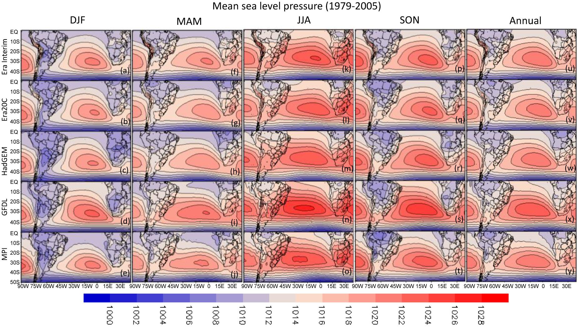
Figure 1. Seasonal and annual climatologies of the mean sea level pressure (hPa) in the present climate (1979–2005) from ERA-Interim (a,f,k,p,u) and ERA-20C (b,g,l,q,v) reanalyses, and HadGEM (c,h,m,r,w), GFDL (d,i,n,s,x), and MPI global climate models (e,j,o,t,y). Isobars interval is 2 hPa.
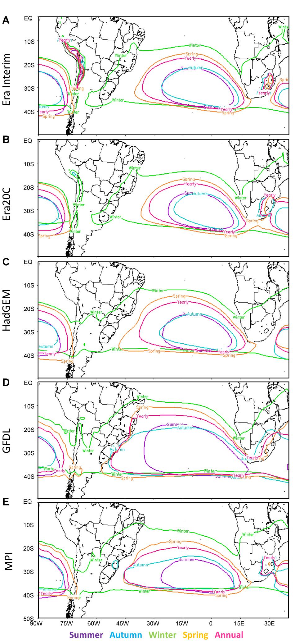
Figure 2. Seasonal and annual climatologies of the 1018 hPa isobar in the present climate (1979–2005) from (A) ERA-Interim, (B) ERA-20C, (C) HadGEM, (D) GFDL, and (E) MPI.
As shown by Reboita et al. (2016a), the validation of the simulations is a hard task once there are differences between the observed data (reanalyses), which can be seen, for example, by comparing ERA-Interim and ERA-20C. Although the seasonal spatial pattern of the SASA is similar in both, the MSLP values (Figure 1) and the area covered by 1018 hPa isobar (Figure 2) are slightly lower in ERA-20C than in ERA-Interim. In this way, the performance of the models can be better or worse depending on the dataset used in the validation. Here, we are considering both reanalyses in the comparisons with the models. The seasonal spatial pattern of the SASA is well simulated by the three models, however, there are some differences in the simulated intensity compared to the reanalyses (Figure 1). While HadGEM overestimates the MSLP in the western sector of the SASA in winter and spring, GFDL overestimates it in all the SASA area and seasons (Figure 1). MPI simulates the SASA with lower meridional amplitude and with the highest-pressure center displaced to the west compared to the reanalyses and simulations (Figure 1). The reported results can also be observed in Figure 2. Considering the 1018 hPa isobar, three simulations show the SASA with a larger area than in the reanalyses. In summary, comparing the performance of the three models, HadGEM is that which simulates the SASA closest to the reanalyses.
For a more detailed evaluation of the SASA position (core with the highest-pressure), we searched the monthly SASA position through an algorithm (see section “Methodology”) and performed the seasonal average of the latitude and longitude. These results and those obtained from the literature are shown in Table 1, while the results of the projections in Table 2. SASA reaches the most northerly position in winter, but its latitude differs in the literature: 27° S in Hastenrath (1991), 28° S in Degola (2013), 29° S in ERA-Interim, ERA-20C and Mächel et al. (1998) and 30° S in Ito and Ambrizzi (2000). Regarding the global climate models, GFDL simulates the northern latitude at 27° S, and HadGEM and MPI at 28° S. Therefore, the models agree with the observations. The most southerly position is registered in summer: 31° S in Hastenrath (1991), Mächel et al. (1998), and Degola (2013), and approximately 32° S in ERA-Interim and ERA-20C (Table 1). MPI simulates the most southerly position in 33° S while GFDL and HadGEM show it in autumn (32.5° S, respectively). In these two models, in summer the SASA position is approximately 32° S. While in the present study (reanalyses and models) the SASA latitude is similar to the literature, the longitude is more variable. SASA is in the most westerly position in winter: 12.6° W in Hastenrath (1991), 11.5° W in Mächel et al. (1998), 11° W in Degola (2013), 7° W in ERA-Interim, and 6° W in ERA-20C. Ito and Ambrizzi (2000) obtained the most westerly position of the SASA in spring (7° W) compared to winter (0°). The models simulate the SASA position displaced to the west in relation to these studies, i.e., 20.8° W in MPI, 19.6° W in GFDL, and 13° W in HadGEM. Although Figure 1 shows the SASA center displaced to east in summer, the highest-pressure center (core) is not necessarily located in the most easterly position in this season. Hastenrath (1991) and Degola (2013) found the most easterly position to the core in autumn (2.3° W and 2.5° W, respectively), and Mächel et al. (1998) in spring (6.6° W). Here, ERA-Interim and ERA-20C registered it in spring (3.9° W) and autumn (2.1° W), respectively. On the other hand, two global climate models simulated the most easterly position in summer (∼6° W in GFDL and MPI), and one in spring (∼6° W in HadGEM).
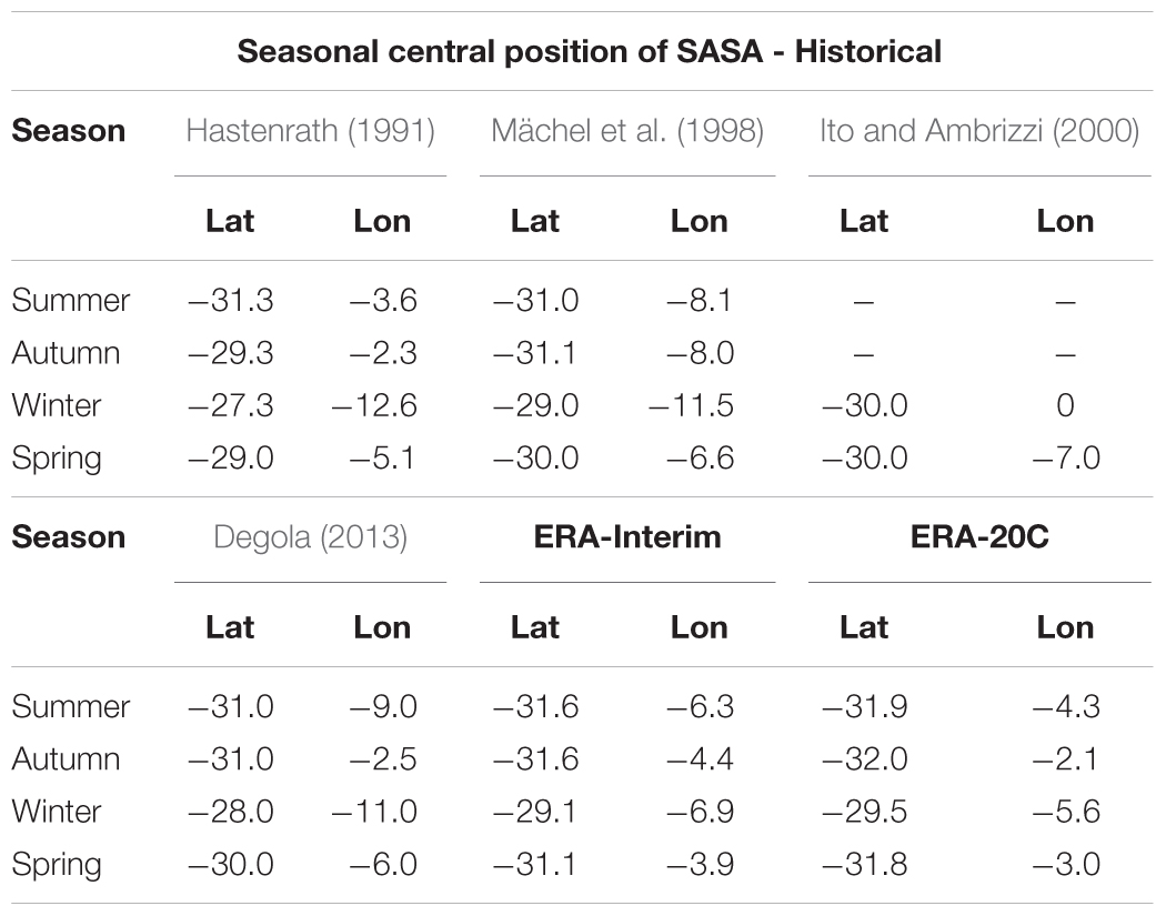
Table 1. Seasonal climatology of the highest SASA pressure center (latitude and longitude) in the present climate (1979–2005) obtained from ERA-Interim, ERA20C and the literature (see text citations).
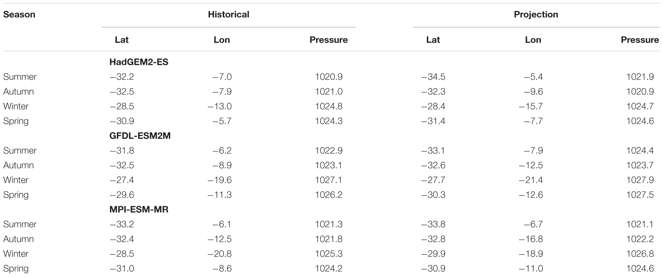
Table 2. Seasonal climatology of the position of the highest SASA pressure center and its pressure (hPa) in the present (1979–2005) and future climate (2065–2095), considering the RCP8.5 scenario.
To provide more details about the monthly position of the SASA core, we constructed graphs (Figure 3) similar to Hastenrath (1991) and Mächel et al. (1998). Models show higher spatial variability of the SASA core compared to the reanalyses. An interesting feature in Figure 3 is the more westerly position of the SASA in February in ERA-Interim and ERA-20C but not in the simulations. This February pattern was also obtained by Mächel et al. (1998) and Degola (2013). It may be caused by the transition of summer to autumn, and it certainly deserves further investigation. Sun et al. (2017), using geopotential height, indicated that the SASA longitudinal variability throughout the year is about 14°, while the latitudinal variability is about 6°. Here, using the MLSP of ERA-Interim and ERA-20C (Figure 3), we found a lower longitudinal variability (approximately 10°), being similar to that obtained by Mächel et al. (1998). For the latitudinal variability, our result is similar to Sun et al. (2017) and Mächel et al. (1998). Regarding the simulations, the longitudinal variability is about 8° higher than the reanalyses while the latitudinal variability is only about 1° (Figure 3).
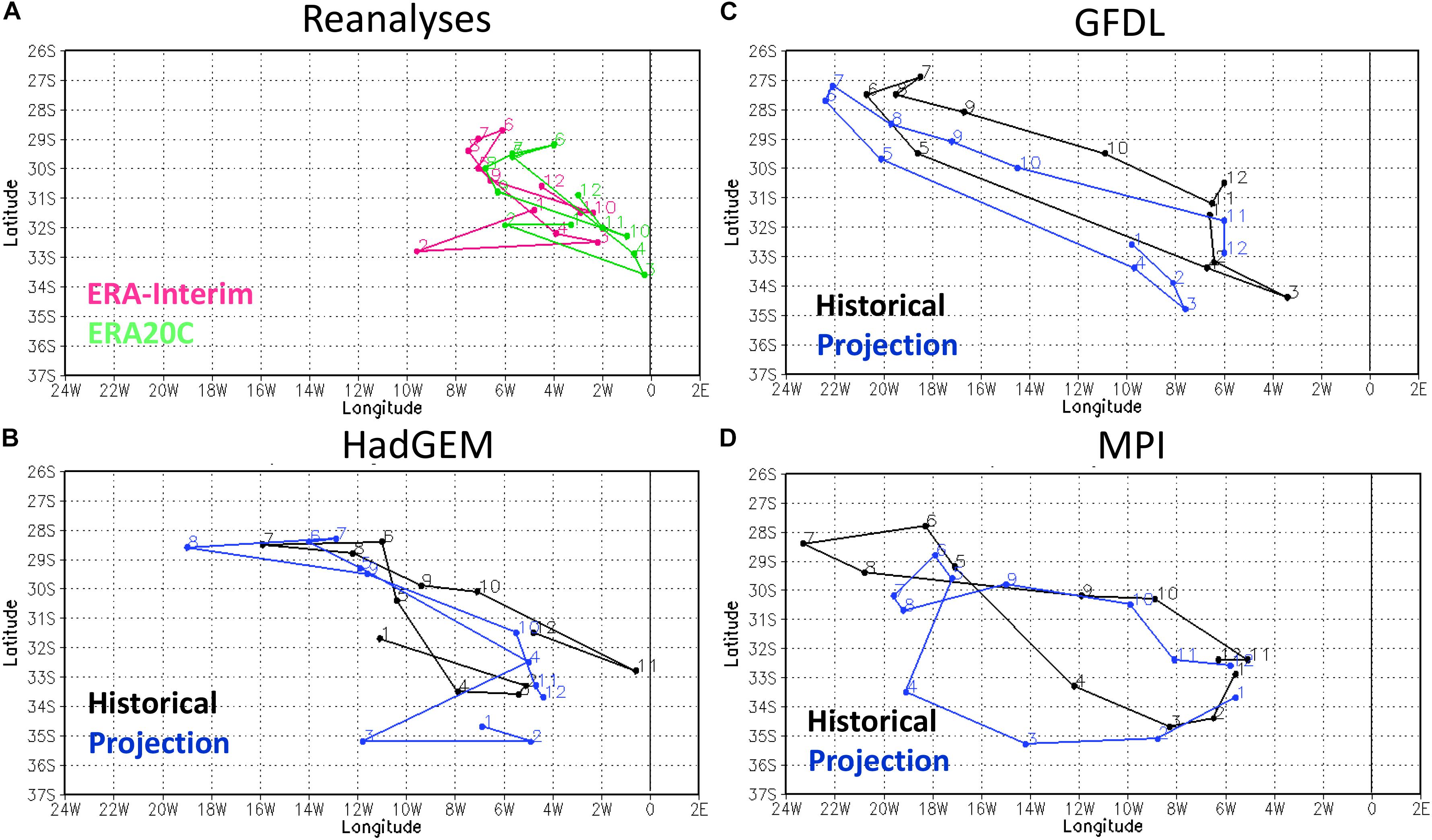
Figure 3. Monthly climatology of the highest SASA pressure center position (latitude and longitude) in the present and future climates (black and blue lines, respectively) from (A) reanalyses (only for present), (B) HadGEM, (C) GFDL, and (D) MPI. Numbers from 1 to 12 refer to the months of the year and the vertical black line indicates the longitude 0°.
In terms of the intensity of the SASA core, in winter the MSLP is about 1024 hPa in ERA-Interim and ERA-20C,1025 hPa in HadGEM and MPI, and 1027 hPa in GFDL (Table 2). These values are lower in summer: 1021 hPa in all datasets, except in GFDL (1023 hPa). Monthly values are shown in Figure 4, and the reanalyses are in agreement with Mächel et al. (1998) and Degola (2013), who indicated that the maximum pressure value does not surpass 1025 hPa in winter and does not decrease less than 1021 hPa in summer. The models reproduce the annual cycle of the MSLP (Figure 4), with HadGEM and MPI showing values similar to the reanalyses, and GFDL overestimating it. To end this section, we present in Figure 5 the scatterplot of the SASA core monthly position. While the reanalyses (Figure 5A) show the more concentrated SASA position, it is more spread westward in the simulations, agreeing with Figure 3. Both reanalyses and models show a negative linear trend, indicating that in the present climate there is a slightly southward displacement of the highest SASA pressure center. In all datasets from Figure 5, Mann–Kendall test indicates that the negative trends are statistically significant at the 0.05 level. This result is concordant with studies that indicate a poleward expansion of the Hadley cell in the present climate, such as Hu and Fu (2007) and Hu et al. (2018), and the associated poleward displacement of the other atmospheric systems like the tropical cyclones (Sharmila and Walsh, 2018).
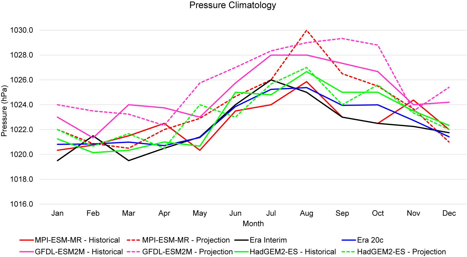
Figure 4. Monthly climatology of the pressure (hPa) of the SASA center.
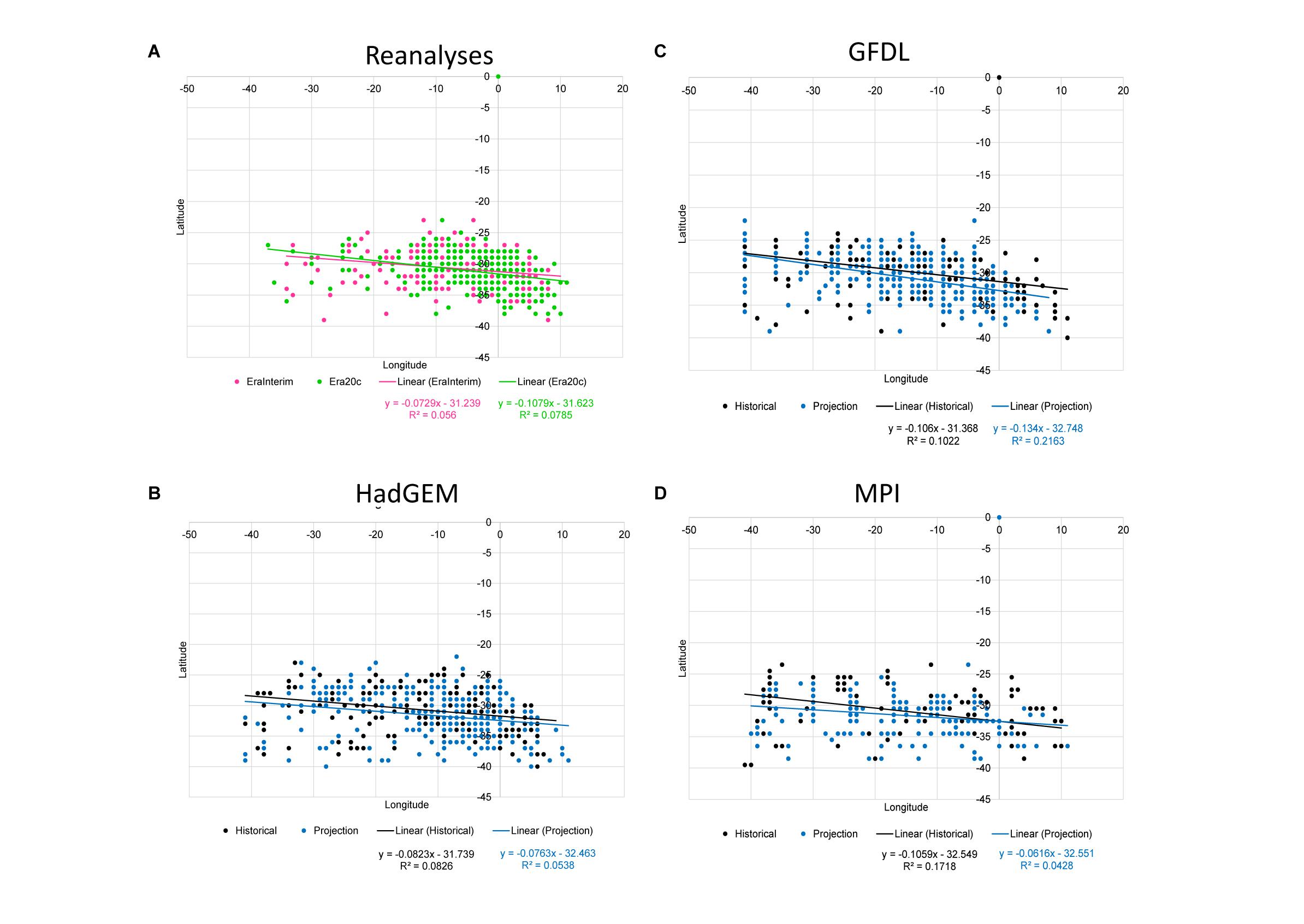
Figure 5. Scatter diagram for monthly latitude and longitude of the SASA in the present and future climates from (A) reanalyses (only for present), (B) HadGEM, (C) GFDL, and (D) MPI. Regression equations are also shown in the plots.
Although the global climate models show some differences in the latitude and longitude of the SASA core, they were able to reproduce the seasonal spatial pattern of this system. This result gives confidence to study the SASA in the climate projections.
Future Climate
Figure 6 shows the seasonal and annual average of the MSLP projected for 2065–2095, while Figure 7 presents the difference between future and present. The spatial pattern of the MSLP (Figure 6) is similar to that of the present climate with the SASA being zonally wider and more intense in winter (Figure 1). However, there are some changes in the MSLP values (Figure 7). In general, an increase in the MSLP in the southern sector of the South Atlantic Ocean and a decrease in the tropical sector, mainly toward Africa, are projected. These changes appear more intense in summer (Figure 7).
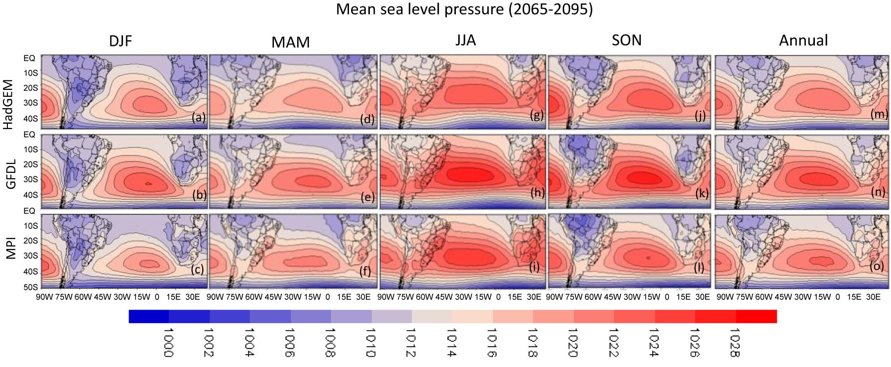
Figure 6. Seasonal and annual climatologies of the mean sea level pressure (hPa) in the future climate (2065–2095) from HadGEM (a,d,g,j,m), GFDL (b,e,h,k,n), and MPI (c,f,i,l,o) global climate models. Isobars interval is 2 hPa.
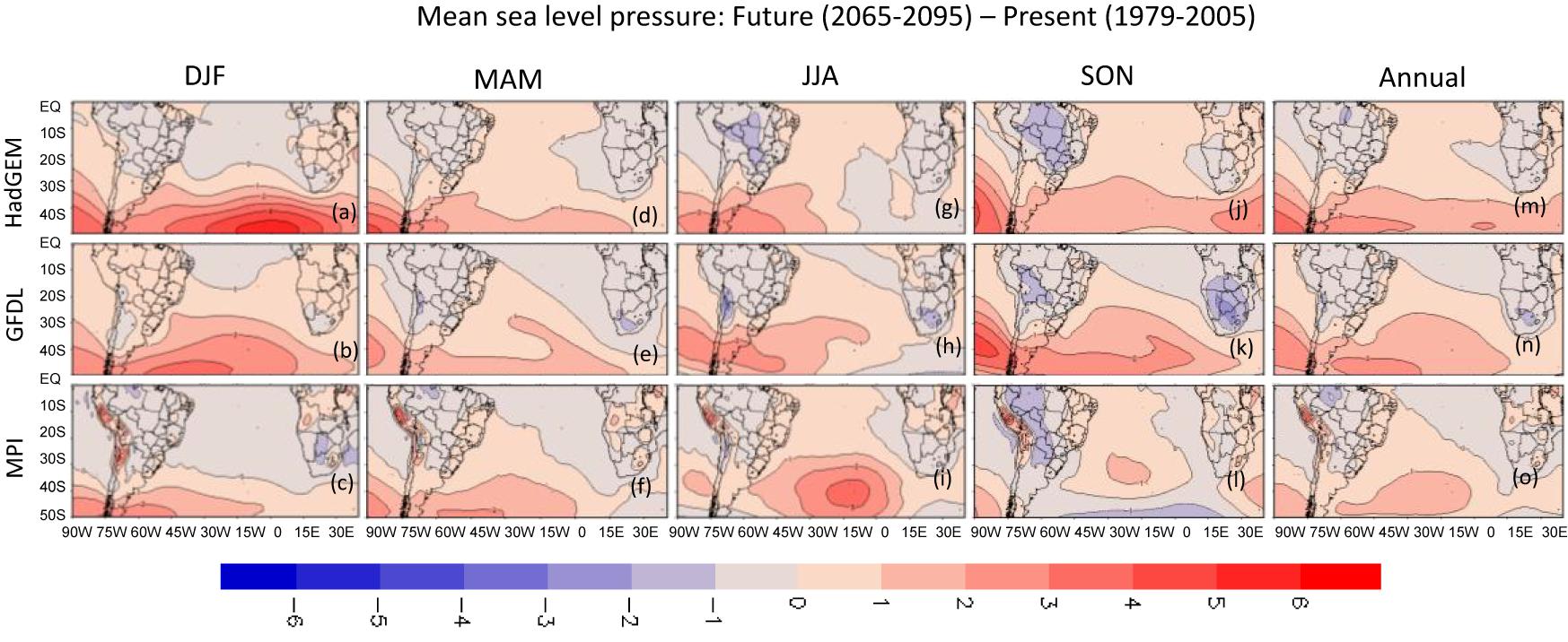
Figure 7. Differences between the mean sea level pressure in the future (2065–2095) and present (1979–2005) climates, for seasonal and annual periods, from HadGEM (a,d,g,j,m), GFDL (b,e,h,k,n), and MPI (c,f,i,l,o) global climate models.
To simplify the evaluation of the MLSP future changes in the SASA, we analyzed the spatial pattern of two specific isobars (1018 and 1020 hPa) in summer and winter (Figure 8). Both isobars indicate that the SASA can become wider due to an expansion westward and southward. Only MPI does not indicate a widening of the SASA in summer in the future (Figures 8C–F). The SASA expansion in the future climate was also obtained by Seth et al. (2010) and Reboita et al. (2017). This expansion seems to influence the position of the highest-pressure center (core) of the SASA (Table 2) once in the RCP8.5 scenario it appears slightly displaced southward in all seasons (except in autumn and winter in HadGEM2) which agrees with He et al. (2017). This feature also appears in the comparison of the monthly SASA position between the present and the future (Figure 3) and in the scatterplot of the SASA position (Figure 5). The slightly southward displacement can be an answer for the changes in the MSLP field shown in Figure 7 (pressure reduction in the tropical sector toward Africa and an increase south of 30° S), which in turn may be a Hadley cell response.
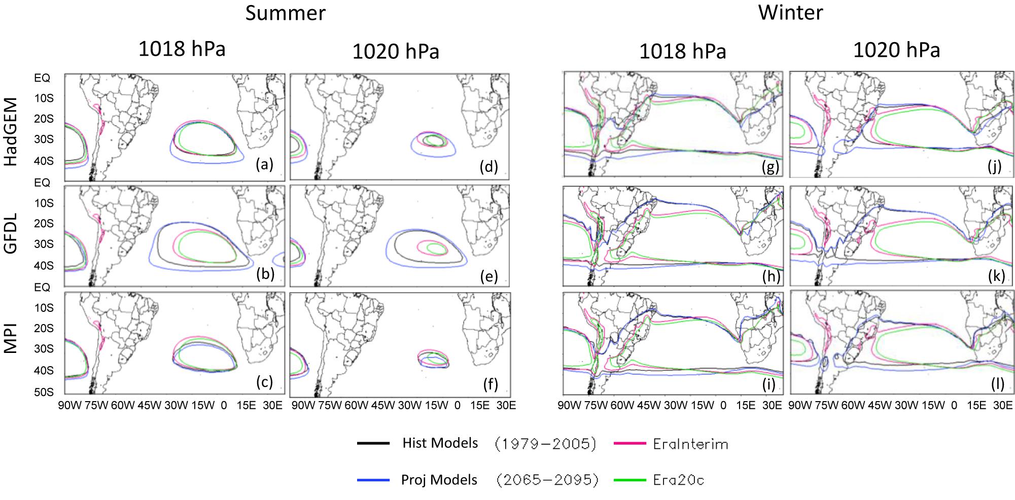
Figure 8. Climatology of the 1018 and 1020 hPa isobars, for summer and winter in the present (1979–2005) and future (2065–2095) climates, from HadGEM (a,d,g,j), GFDL (b,e,h,k), and MPI (c,f,i,l). Reanalyses are also presented.
The projection of the SASA core intensity is similar to the present or slightly higher (Table 2 and Figure 4), differing from He et al. (2017), who found a weakening of the SASA in the future climate. The projections reproduce the annual cycle of the MSLP registered in the present climate (Figure 4), but with the GFDL showing higher pressure values.
To know more about the SASA vertical structure, latitude-height cross sections of the vertical velocity (omega) considering the future and present climate and the difference between them are presented for summer (Figure 9) and winter (Figure 10). The longitude used in the cross sections is that identified by the algorithm in the present climate (Table 2). The SASA is represented by a descending motion (positive values in the vertical velocity). Figures 9, 10 are also a representation of the atmospheric circulation in the Southern Hemisphere, which includes the Hadley cell. This cell is a thermally direct tropospheric circulation with the rising motion of warm air near the equator and a descending motion in the subtropics in both hemispheres. Therefore, the polar branch of the Hadley cell is one of the main drivers of the SASA (Rodwell and Hoskins, 2001; Dima and Wallace, 2003; Seager et al., 2003), consequently, changes in this cell affect the SASA.
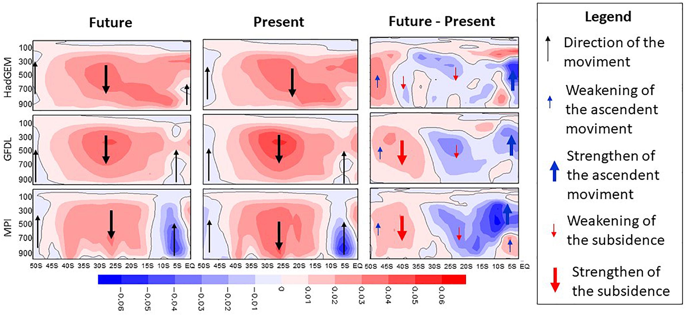
Figure 9. Latitude-height cross sections of the vertical velocity (omega; Pa s-1) in summer for the future, present and the difference future minus present. The black line indicates the zero value.
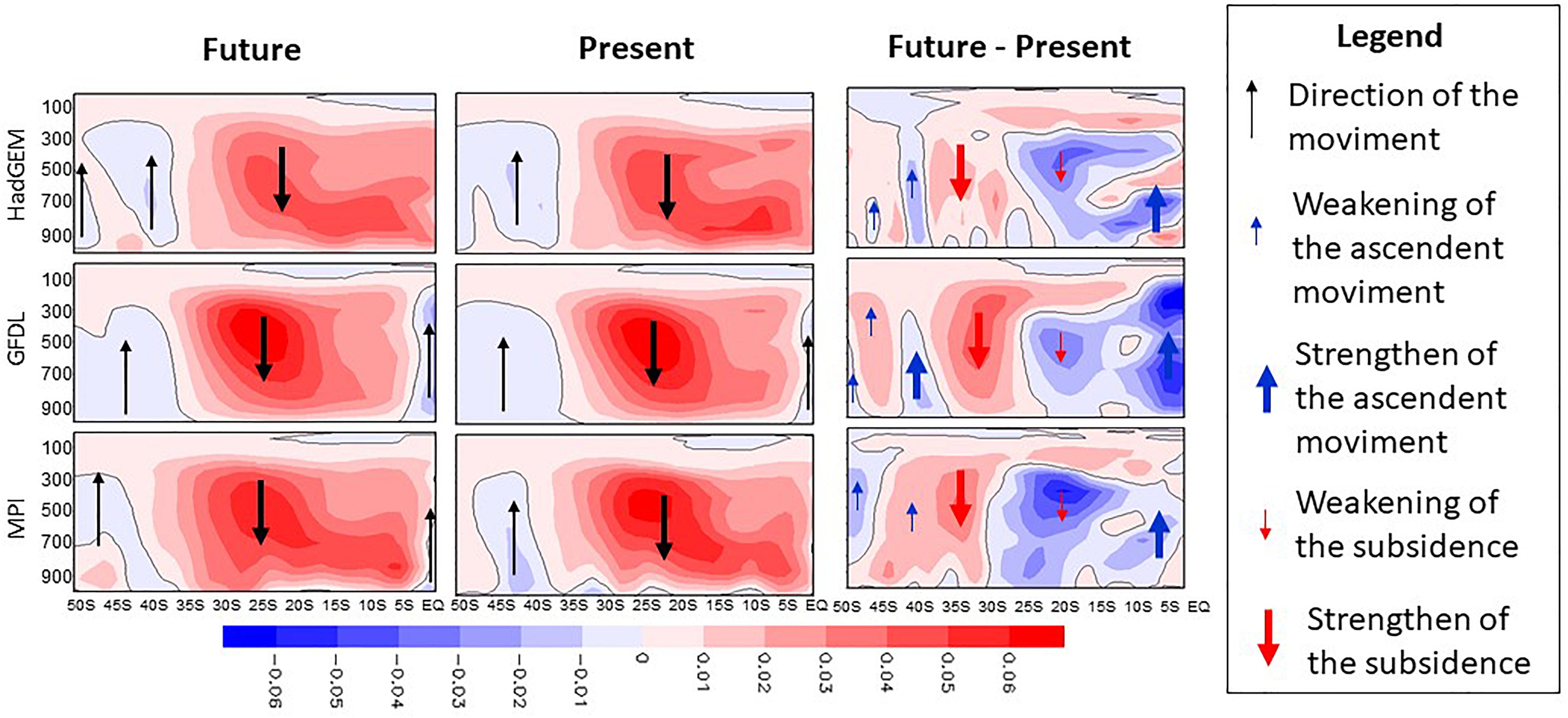
Figure 10. Similar to Figure 9 but for winter.
Figures 9, 10 show a decrease in the subsidence in the RCP8.5 scenario, in general between 20° and 30° S, and an increase at higher latitudes (until ∼45° S in summer and 40° S in winter). Therefore, this result agrees with the literature in which there will be a poleward expansion of the Hadley cell (Deser and Phillips, 2009; Son et al., 2009, 2010; Polvani et al., 2011; Nguyen et al., 2013, 2015; Allen et al., 2014; Davis et al., 2016; Grise and Polvani, 2016; Tao et al., 2016; Hu et al., 2018) and, consequently, of the SASA. Comparing summer and winter (Figures 9, 10), in winter the subsidence associated with the Hadley cell is more intense and reaches lower latitudes.
The poleward expansion of the Hadley cell is documented for the present climate and future projections. In the present climate, different reanalyses show an expansion of about 1° in latitude per decade (Hu and Fu, 2007; Hu et al., 2018), while CMIP5 historical simulations underestimate it, showing an expansion that ranges from 0.17° (Hu et al., 2013) to 0.2° (Tao et al., 2016) in latitude per decade. For the future climate, the expansion increases to about 0.27° in latitude per decade (Hu et al., 2013). But what are the causes of the Hadley cell expansion? Some numerical experiments indicate that this expansion is associated with the stratospheric ozone depletion (Son et al., 2009, 2010; Polvani et al., 2011; Min and Son, 2013; Waugh et al., 2015), the increase of the greenhouse gasses (Allen et al., 2012; Nguyen et al., 2015; Davis et al., 2016) or by both forcings (Tao et al., 2016). On the other hand, natural forcing or anthropogenic aerosols do not generate significant trends in the Hadley cell expansion (Tao et al., 2016).
The mentioned forcings firstly affect the horizontal temperature gradients (the physical mechanisms that explain this are not fully known), that become displaced poleward. It has an impact in the global atmospheric circulation with a poleward displacement of the upper level jets and storm tracks (Catto, 2016; Reboita et al., 2018) and an expansion of Halley cell (Lu et al., 2007, 2008; Hu et al., 2013, 2018; Lucas et al., 2014; Seo et al., 2014; Lau and Kim, 2015; Nguyen et al., 2015; Davis et al., 2016; Grise and Polvani, 2016; Tao et al., 2016; Lipat et al., 2017). This expansion can be associated with the ability of the Hadley cell to maintain angular momentum conservation in front of the poleward displacement of the other systems (Korty and Schneider, 2008). In this way, in climate scenarios, latitudes toward the extratropical region will present higher pressure than in the present climate and it may explain the increase of the surface pressure toward the mid-latitudes reported in Figure 7.
In terms of the more intense changes in the surface pressure showed in summer (Figure 7), it may be a relation with the higher stratospheric ozone depletion in this same season (Son et al., 2009, 2010; Polvani et al., 2011; Min and Son, 2013; Waugh et al., 2015). The ozone depletion is a consequence of strong stratospheric vortex that difficulties the exchange of the polar air with midlatitudes during winter and spring. Then, the ozone is more easily consumed during these seasons reaching the maximum depletion in summer (Pazmiño et al., 2005; Davis et al., 2016). The ozone depletion causes a cooling of the stratosphere in high latitudes leading to more intense meridional temperature gradients between the tropospheric polar region and the extratropics (Polvani et al., 2011). It helps the poleward displacement of the westerly winds and the Haddley cell in summer. Therefore, these results may provide a possible explanation of why surface pressure is higher in summer as indicated in Figure 7.
Conclusion
This study complements the work of He et al. (2017), providing a regional point of view of the South Atlantic Subtropical Anticyclone (SASA). Moreover, a thorough review of the literature was also done, in order to better discuss the semi-permanent anticyclones maintenance.
The SASA seasonal variability is characterized by a wider zonally and intense system during the winter. Regressing analysis using present climate data indicates a small, but statistically significant, trend of the southward displacement of the SASA core. These features were well reproduced by the CMIP5 models (MPI-ESM-MR, HadGEM2-ES and GFDL-ESM2M) in the present climate with HadGEM2-ES showing more similarities with the reanalyses.
In terms of climate projections, the main results are:
• Regarding the MSLP spatiality, an increase of the MSLP in the south sector of the South Atlantic Ocean and a decrease in the tropical sector, mainly toward Africa, are projected;
• The area of the SASA shows an expansion southward and westward compared to the present climate;
• The SASA core (the highest-pressure position) presents a slightly, but statistically significant, southward displacement in future climate scenarios, and
• The SASA core intensity does not show any significant change in the future.
We suggest that the changes projected for the SASA are directly related to the southward expansion of the Hadley cell, which in turn is associated with the changes in the horizontal temperature gradients (Lu et al., 2007, 2008; Allen et al., 2012; and see a review in Reboita et al., 2018) in climate change scenarios. Therefore, the poleward shift of the Hadley cell and the storm tracks will affect the SASA.
It is important to emphasize that projections have uncertainties, which are associated with different models, physical parameterizations etc., generating different climate responses (see, for instance, Cherchi et al., 2018). However, besides the uncertainties, this study is relevant to indicate possible changes in the future climate providing a guidance to the decision makers to implement measures of mitigation and/or adaptation. For example, the SASA expansion can shift dry zones southward, which will have an impact on agriculture, energy, population health, and others.
Author Contributions
BS and RP worked together to prepare the data and plots while MR, TA, and RdR discussed ideas and wrote the manuscript.
Funding
TA was supported by the National Institute of Science and Technology for Climate Change Phase 2 under CNPq Grant 465501/2014-1, FAPESP Grants 2014/50848-9, the National Coordination for High Level Education and Training (CAPES) Grant 16/2014, and FAPESP Grant PACMEDY Project 2015/50686.
Conflict of Interest Statement
The authors declare that the research was conducted in the absence of any commercial or financial relationships that could be construed as a potential conflict of interest.
Acknowledgments
We wish to acknowledge all the modeling groups of CMIP5 and ECMWF by the reanalyses. We thank CNPq, CAPES, FAPESP, and FAPEMIG by the financial support.
References
Alkama, R., Marchand, L., Ribes, A., and Decharme, B. (2013). Detection of global runoff changes: results from observations and CMIP5 experiments. Hydrol. Earth Syst. Sci. 17, 2967–2979. doi: 10.5194/hess-17-2967-2013
Allen, R. J., Norris, J. R., and Kovilakam, M. (2014). Influence of anthropogenic aerosols and the Pacific Decadal Oscillation on tropical belt width. Nat. Geosci. 7, 270–274. doi: 10.1038/ngeo2091
Allen, R. J., Sherwood, S. C., Norris, J. R., and Zender, C. S. (2012). Recent Northern Hemisphere tropical expansion primarily driven by black carbon and tropospheric ozone. Nature 485, 350–354. doi: 10.1038/nature11097
Cabos, W., Sein, D. V., Pinto, J. G., Fink, A. H., Koldunov, N. V., Alvarez, F., et al. (2017). The South Atlantic Anticyclone as a key player for the representation of the tropical Atlantic climate in coupled climate models. Clim. Dyn. 48, 4051–4069. doi: 10.1007/s00382-016-3319-9
Catto, J. L. (2016). Extratropical cyclone classification and its use in climate studies. Rev. Geophys. 54, 486–520. doi: 10.1002/2016RG000519
Chen, P. C., Hoerling, M. P., and Dole, R. M. (2001). The origin of the subtropicalanticyclones. J. Atmos. Sci. 58, 1827–1835. doi: 10.1038/srep21346
Cherchi, A., Ambrizzi, T., Behera, S., Freitas, A. C. V., Morioka, Y., and Zhou, T. (2018). The response of subtropical highs to climate change. Curr. Clim. Chang. Rep. 4, 371–382. doi: 10.1007/s40641-018-0114-1
Choi, J., Son, S. W., Lu, J., and Min, S. K. (2014). Further observational evidence of Hadley cell widening in the Southern Hemisphere. Geophys. Res. Lett. 41, 2590–2597. doi: 10.1002/2014GL059426
Coelho, C. A. S., Oliveira, C. P., Ambrizzi, T., Reboita, M. S., Carpenedo, C. B., Campos, J. L. P. S., et al. (2016). The 2014 southeast Brazil austral summer drough: regional scale mechanisms and teleconnections. Clim. Dyn. 46, 3737–3752. doi: 10.1007/s00382-015-2800-1
Correa, T. S., Reboita, M. S., and Carvalho, V. S. B. (2018). Investigação da Relação entre Variáveis Atmosféricas e a Concentração de MP10 e O3 no Estado de São Paulo. Rev. Bras. Meteorol. (in press).
Davis, N. A., Seidel, D. J., Birner, T., Davis, S. M., and Tilmes, S. (2016). Changes in the width of the tropical belt due to simple radiative forcing changes in the GeoMIP simulations. Atmos. Chem. Phys. 16, 10083–10095. doi: 10.5194/acp-16-10083-2016
Dee, D. P., Uppala, S. M., Simmons, A. J., Berrisford, P., Poli, P., Kobayashi, S., et al. (2011). The ERA-Interim reanalysis: configuration and performance of the data assimilation system. Q. J. R. Meteorol. Soc. 137, 553–597. doi: 10.1002/qj.828
Degola, T. S. D. (2013). Impacts and Variability of the South Atlantic Subtropical Anticyclone on Brazil in the Present Climate and in Future Scenarios. Dissertation/master’s thesis, University of São Paulo, São Paulo.
Deser, C., and Phillips, A. S. (2009). Atmospheric circulation trends, 1950–2000: the relative roles of sea surface temperature forcing and direct atmospheric radiative forcing. J. Clim. 22, 396–413. doi: 10.1175/2008JCLI2453.1
Dima, I. M., and Wallace, J. M. (2003). On the seasonality of the Hadley cell. J. Atmos. Sci. 60, 1522–1527. doi: 10.1175/1520-0469(2003)060<1522:OTSOTH>2.0.CO;2
Dunne, J. P., John, J. G., Adcroft, A. J., Griffies, S. M., Hallberg, R. W., Shevliakova, E., et al. (2012). GFDL’s ESM2 global coupled climate–carbon earth system models. Part I: physical formulation and baseline simulation characteristics. J. Clim. 25, 6646–6665. doi: 10.1175/JCLI-D-11-00560.1
Gilliland, J. M., and Keim, B. D. (2018a). Position of the South Atlantic Anticyclone and its impact on surface conditions across Brazil. J. Appl. Meteorol. Clim. 57, 535–553. doi: 10.1175/JAMC-D-17-0178.1
Gilliland, J. M., and Keim, B. D. (2018b). Surface wind speed: trend and climatology of Brazil from 1980–2014. Int. J. Climatol. 38, 1060–1073. doi: 10.1002/joc.5237
Giorgetta, M. A., Jungclaus, J., Reick, C. H., Legutke, S., Bader, J., Böttinger, M., et al. (2013). Climate and carbon cycle changes from 1850 to 2100 in MPI-ESM simulations for the Coupled Model Intercomparison Project phase 5. J. Adv. Model. Earth Syst. 5, 572–597. doi: 10.1002/jame.20038
Giorgi, F., Jones, C., and Asrar, G. (2009). Addressing climate information needs at the regional level: the CORDEX framework. World Meteorol. Org. Bull. 58, 175–183.
Grise, K. M., and Polvani, L. M. (2016). Is climate sensitivity related to dynamical sensitivity? J. Geophys. Res: Atmos. 121, 5159–5176. doi: 10.1002/2015JD024687
Guo, Y.-P., Li, J.-P., and Feng, J. (2016). Climatology and interannual variability of the annual mean Hadley circulation in CMIP5 models. Adv. Clim. Chang. Res. 7, 35–45. doi: 10.1016/j.accre.2016.04.005
Hastenrath, S. (1991). Climate Dynamics of the Tropics. Berlin: Springer. doi: 10.1007/978-94-011-3156-8
He, C., Wu, B., Zou, L., and Zhou, T. (2017). Responses of the summertime subtropical anticyclones to global warming. J. Clim. 30, 6465–6479. doi: 10.1175/JCLI-D-16-0529.1
Hu, Y., and Fu, Q. (2007). Observed poleward expansion of the Hadley circulation since 1979. Atmos. Chem. Phys. 7, 5229–5236. doi: 10.5194/acp-7-5229-2007
Hu, Y., Huang, H., and Zhou, C. (2018). Widening and weakening of the Hadley circulation under global warming. Sci. Bull. 63, 640–644. doi: 10.1016/j.scib.2018.04.020
Hu, Y., Tao, L., and Liu, J. (2013). Poleward expansion of the Hadley circulation in CMIP5 simulations. Adv. Atmos. Sci. 30, 790–795. doi: 10.1073/pnas.1811068115
Ioannidou, L., and Yau, M. K. (2008). A climatology of the Northern Hemisphere winter anticyclones. J. Geophys. Res. 113:D08119. doi: 10.1029/2007JD008409
Ito, E. R. K. (1999). A Climatological Study of the South Atlantic Subtropical Anticyclone and its Influence on Frontal Systems. Institute of Astronomy. Dissertation/master’s thesis, University of São Paulo, São Paulo.
Ito, E. R. K., and Ambrizzi, T. (2000). “Climatology of subtropical high position of the South Atlantic Ocean for the winter months,” in Annals of the XI Latin American and Iberian Congress of Meteorology, Buenos Aires, 860–865.
Ji, X., Neelin, J. D., Lee, S. K., and Mechoso, C. R. (2014). Interhemispheric teleconnections from tropical heat sources in intermediate and simple models. J. Clim. 27, 684–697. doi: 10.1175/JCLI-D-13-00017.1
Joetzjer, E., Douville, H., Delire, C., and Ciais, P. (2013). Present-day and future Amazonian precipitation in global climate models: CMIP5 versus CMIP3. Clim. Dyn. 41, 2921–2936. doi: 10.1007/s00382-012-1644-1
Jones, C. D., Hughes, J. K., Bellouin, N., Hardiman, S. C., Jones, G. S., Knight, J., et al. (2011). The HadGEM2-ES implementation of CMIP5 centennial simulations. Geosci. Model. Dev. 4, 543–570. doi: 10.5194/gmd-4-543-2011
Josey, S. A., Kent, E. C., and Taylor, P. K. (1998). The Southampton Oceanography Centre (SOC) Ocean-Atmosphere Heat, Momentum and Freshwater Flux Atlas. Southampton: Southampton Oceanography Centre.
Kim, Y.-H., Min, S.-K., Son, S.-K., and Choi, J. (2017). Attribution of local Hadleycell widening in the southern hemisphere. Geophys. Res. Lett. 44, 1015–1024. doi: 10.1002/2016GL072353
Korty, R. L., and Schneider, T. (2008). Extent of Hadley circulations in dry atmospheres. Geophys. Res. Lett. 35:L23803. doi: 10.1029/2008GL035847
Kosaka, Y., and Nakamura, H. (2010). Mechanisms of meridional teleconnection observed between a summer monsoon system and a subtropical anticyclone. Part II: a global survey. J. Clim. 23, 5109–5125. doi: 10.1175/2010JCLI3414.1
Lambert, S. J. (1988). A cyclone climatology of the Canadian centre general circulation model. J. Clim. 1, 109–115. doi: 10.1175/1520-0442(1988)001<0109:ACCOTC>2.0.CO;2
Lau, W. K., and Kim, K. M. (2015). Robust Hadley circulation changes and increasing global dryness due to CO2 warming from CMIP5 model projections. Proc. Natl. Acad. Sci. U.S.A. 112, 3630–3635. doi: 10.1073/pnas.1418682112
Lee, S. K., Mechoso, C. R., Wang, C., and Neelin, J. D. (2013). Interhemispheric influence of the northern summer monsoons on southern subtropical anticyclones. J. Clim. 26, 10193–10204. doi: 10.1175/JCLI-D-13-00106.1
Lipat, B. R., Tselioudis, G., Grise, K. M., and Polvani, L. M. (2017). CMIP5 models’ shortwave cloud radiative response and climate sensitivity linked to the climatological Hadley cell extent. Geophys. Res. Lett. 44, 5739–5748. doi: 10.1002/2017GL073151
Liu, Y., Wu, G., and Ren, R. (2004). Relationship between the subtropical anticyclone and diabatic heating. J. Clim. 17, 682–698. doi: 10.1175/1520-0442(2004)017<0682:RBTSAA>2.0.CO;2
Lu, J., Chen, G., and Frierson, D. M. W. (2008). Response of the zonal mean atmospheric circulation to el niño versus global warming. J. Clim. 15, 5835–5851. doi: 10.1175/2008JCLI2200.1
Lu, J., Vecchi, G., and Reichler, T. (2007). Expansion of the Hadley cell under global warming. Geophys. Res. Lett. 34:L06805. doi: 10.1029/2006GL028443
Lucas, C., and Nguyen, H. (2015). Regional characteristics of tropical expansion and the role of climate variability. J. Geophys. Res. Atmos. 120, 6809–6824. doi: 10.1002/2015JD023130
Lucas, C., Timbal, B., and Nguyen, H. (2014). The expanding tropics: a critical assessment of the observational and modeling studies. WIREs Clim. Chang. 5, 89–112. doi: 10.1002/wcc.251
Mächel, H., Kapala, A., and Flohn, H. (1998). Behaviour of the centers of action above the Atlantic since 1881. Part I: characteristics of seasonal and interannual variability. Int. J. Climatol. 18, 1–22. doi: 10.1002/(SICI)1097-0088(199801)18:1<1::AID-JOC225>3.0.CO;2-A
Min, S., and Son, S. (2013). Multimodel attribution of the Southern Hemisphere Hadley cell widening: major role of ozone depletion. J. Geophys. Res. 118, 3007–3015. doi: 10.1002/jgrd.50232
Miyasaka, T., and Nakamura, H. (2010). Structure and mechanisms of the Southern Hemisphere summertime subtropical anticyclones. J. Clim. 23, 2115–2130. doi: 10.1175/2009JCLI3008.1
Moss, R. H., Edmonds, J. A., Hibbard, K. A., Manning, M. R., Rose, S. K., Van Vuuren, D. P., et al. (2010). The next generation of scenarios for climate change research and assessment. Nature 463, 747–756. doi: 10.1038/nature08823
Murray, R. J., and Simmonds, I. (1991). A numerical scheme for tracking cyclone centres from digital data. Austr. Meteorol. Mag. 39, 155–166.
Namias, J. (1972). Influence of northern hemisphere general circulation on drought in northeast Brazil 1. Tellus 24, 336–343. doi: 10.3402/tellusa.v24i4.10648
Nguyen, H., Evans, A., Lucas, C., Smith, I., and Timbal, B. (2013). The Hadley circulation in reanalyses: climatology, variability, and expansion. J. Clim. 26, 3357–3376. doi: 10.1175/JCLI-D-12-00224.1
Nguyen, H., Lucas, C., Evans, A., Timbal, B., and Hanson, L. (2015). Expansion of the Southern Hemisphere Hadley cell in response to greenhouse gas forcing. J. Clim. 28, 8067–8077. doi: 10.1175/JCLI-D-15-0139.1
Pazmiño, A. F., Godin-Beekmann, S., Ginzburg, M., Bekki, S., Hauchecorne, A., Piacentini, R. D., et al. (2005). Impact of Antarctic polar vortex occurrences on total ozone and UVB radiation at southern Argentinean and Antarctic stations during 1997–2003 period. J. Geophys. Res. 110, 1–13. doi: 10.1029/2004jd005304
Pepler, A., Dowdy, A., and Hope, P. (2018). A Global Climatology of Surface Anticyclones, their Variability, Associated Drivers and Long-term Trends. Berlin: Springer-Verlag, doi: 10.1007/s00382-018-4451-5
Peterson, R. G., and Stramma, L. (1991). Upper-level circulation in the South Atlantic Ocean. Progr. Oceanogr. 26, 1–73. doi: 10.1016/0079-6611(91)90006-8
Pezza, A. B., and Ambrizzi, T. (2005). Dynamical conditions and synoptic tracks associated with different types of cold surge over tropical South America. Int. J. Climatol. 25, 215–241. doi: 10.1002/joc.1080
Poli, P., Hersbach, H., Dee, D. P., Berrisford, P., Simmons, A. J., Vitart, F., et al. (2016). ERA-20C: an atmospheric reanalysis of the twentieth century. J. Clim. 29, 4083–4097. doi: 10.1175/JCLI-D-15-0556.1
Polvani, L. M., Waugh, D. W., Correa, G. J., and Son, S. W. (2011). Stratospheric ozone depletion: the main driver of twentieth-century atmospheric circulation changes in the Southern Hemisphere. J. Clim. 24, 795–812. doi: 10.1175/2010JCLI3772.1
Reboita, M. S., Amaro, T. R., and de Souza, M. R. (2017). Winds: intensity and power density simulated by RegCM4 over South America in present and future climate. Clim. Dyn. 51, 187–205. doi: 10.1007/s00382-017-3913-5
Reboita, M. S., da Rocha, R. P., de Souza, M. R., and Llopart, M. (2018). Extratropical cyclones over the southwestern South Atlantic Ocean: HadGEM2-ES and RegCM4 projections. Int. J. Climatol. 38, 2866–2879. doi: 10.1002/joc.5468
Reboita, M. S., Dutra, L. M. M., and Dias, C. G. (2016a). Diurnal cycle of precipitation simulated by RegCM4 over South America: present and future scenarios. Clim. Res. 70, 39–55. doi: 10.3354/cr01416
Reboita, M. S., Gan, M. A., da Rocha, R. P., and Ambrizzi, T. (2010). Regimes of precipitation in South America: a bibliographical review. Braz. J. Meteorol. 25, 185–204. doi: 10.1590/S0102-77862010000200004
Reboita, M. S., Rodrigues, M., Pereira, R. A. A., Freitas, C. H., and Oliveira, G. M. (2016b). Causes of Semi-Aridity in the Northeastern Sertão. Braz. J. Climatol. 19, 254–277.
Reboita, M. S., Rodrigues, M., Silva, L. F., and Alves, M. A. (2015). Climatic Aspects of the State of Minas Gerais. Braz. J. Climatol. 17, 209–229.
Riahi, K., Rao, S., Krey, V., Cho, C., Chirkov, V., Fischer, G., et al. (2011). RCP 8.5 - A scenario of comparatively high greenhouse gas emissions. Climat. Chang. 109:33. doi: 10.1007/s10584-011-0149-y
Ribeiro, F. N. D., de Souza, L. A. T., Salinas, D. T. P., Soares, J., Oliveira, A. P., and Miranda, R. J. (2015). “Air quality in São Paulo – Brazil: temporal evolution and spatial distribution of carbon monoxide, coarse particulate matter and ozone,” in 9th International Conference on Urban Climate jointly with 12th Symposium on the Urban Environment, Toulouse.
Richter, I., Mechoso, C. R., and Robertson, A. W. (2008). What determines the position and intensity of the South Atlantic anticyclone in austral winter? An AGCM study. J. Clim. 21, 214–229. doi: 10.1175/2007JCLI1802.1
Rodwell, M. J., and Hoskins, B. J. (1996). Monsoons and the dynamics of deserts. Q. J. R. Meteorol. Soc. 22, 1385–1404. doi: 10.1002/qj.49712253408
Rodwell, M. J., and Hoskins, B. J. (2001). Subtropical anticyclones and summer monsoons. J. Clim. 14, 3192–3211. doi: 10.1038/srep21346
Rozante, J. R., Rozante, V., Souza Alvim, D., Ocimar Manzi, A., Barboza Chiquetto, J., Siqueira, D., et al. (2017). Variations of Carbon Monoxide Concentrations in the Megacity of São Paulo from 2000 to 2015 in Different Time Scales. Atmosphere 8:81. doi: 10.3390/atmos8050081
Santos, D. F., Martins, F. B., and Torres, R. R. (2017). Impacts of climate projections on water balance and implications on olive crop in Minas Gerais. Rev. Bras. Engenharia Agrícola e Ambiental 21, 77–82. doi: 10.1590/1807-1929/agriambi.v21n2p77-82
Seager, R., Murtugudde, R., Naik, N., Clement, A., Gordon, N., and Miller, J. (2003). Air–sea interaction and the seasonal cycle of the subtropical anticyclones. J. Clim. 16, 1948–1966. doi: 10.1175/1520-0442(2003)016<1948:AIATSC>2.0.CO;2
Seo, K. H., Frierson, D. M., and Son, J. H. (2014). A mechanism for future changes in Hadley circulation strength in CMIP5 climate change simulations. Geophys. Res. Lett. 41, 5251–5258. doi: 10.1073/pnas.1811068115
Seth, A., Rojas, M., and Rauscher, S. A. (2010). CMIP3 projected changes in the annual cycle of the South American monsoon. Clim. Chang. 98, 331–357. doi: 10.1007/s10584-009-9736-6
Shaffrey, L. C., Hoskins, B. J., and Lu, R. (2002). The relationship between theNorth American summer monsoon, the Rocky Mountains andthe North Pacific subtropical anticyclone in HadAM3. Q. J. R. Meteor Soc. 128, 2607–2622. doi: 10.1256/qj.01.145
Sharmila, S., and Walsh, K. J. E. (2018). Recent poleward shift of tropical cyclone formation linked to Hadley cell expansion. Nat. Clim. Chang. 8, 730–736. doi: 10.1038/s41558-018-0227-5
Silva, L. J., Reboita, M. S., and da Rocha, R. P. (2014). Relation of the passage of cold fronts in the southern region of Minas Gerais (RSMG) with precipitation and frost events. Braz. J. Climatol. 14, 229–246.
Sinclair, M. R. (1994). A diagnostic model for estimating orographic precipitation. J. Appl. Meteor. 33, 1163–1175. doi: 10.1175/1520-0450(1994)033<1163:ADMFEO>2.0.CO;2
Sinclair, M. R. (1996). A Climatology of Anticyclones and Blocking for the Southern Hemisphere. Vol. 124, Wellington: National Institute of Water and Atmospheric Research Ltd., 245–264. doi: 10.1175/1520-0493(1996)124<0245:ACOAAB>2.0.CO;2
Son, S. W., Gerber, E. P., Perlwitz, J., Polvani, L. M., Gillett, N. P., Seo, K. H., et al. (2010). Impact of stratospheric ozone on Southern Hemisphere circulation change: a multimodel assessment. J. Geophys. Res. 115, 1–18. doi: 10.1029/2010JD014271
Son, S. W., Tandon, N. F., Polvani, L. M., and Waugh, D. W. (2009). Ozone hole and Southern Hemisphere climate change. Geophys. Res. Lett. 36, 1–5. doi: 10.1029/2009GL038671
Sugahara, S. (2000). “Annual Variation of the Frequency of Cyclones in the South Atlantic Ocean,” in Proceedings of the XI Brazilian Congress of Meteorology, Rio de Janeiro, RJ.
Sun, X., Cook, K. H., and Vizy, E. K. (2017). The South Atlantic subtropical high: climatology and interannual variability. J. Clim. 30, 3279–3296. doi: 10.1175/JCLI-D-16-0705.1
Tao, L., Hu, Y., and Liu, J. (2016). Anthropogenic forcing on the Hadley circulation in CMIP5 simulations. Clim. Dyn. 46, 3337–3350. doi: 10.1007/s00382-015-2772-1
Taylor, K. E., Stouffer, R. J., and Meehl, G. A. (2012). An overview of CMIP5 and the experiment design. Bull. Am. Meteorol. Soc. 93, 485–498. doi: 10.1175/BAMS-D-11-00094.1
van Vuuren, D. P., Edmonds, J., Kainuma, M., Riahi, K., Thomson, A., Hibbard, K., et al. (2011). The representative concentration pathways: an overview. Climat. Chang. 109:5. doi: 10.1007/s10584-011-0148-z
Vianello, R. L., and Maia, L. P. G. (1986). “Preliminary study of the dynamic climatology of the State of Minas Gerais,” in Proceedings of the 4th Brazilian Congress of Meteorology, Brasília.
Keywords: South Atlantic Subtropical Anticyclone, Hadley cell, climate change, RCP8.5, CMIP5 models
Citation: Reboita MS, Ambrizzi T, Silva BA, Pinheiro RF and da Rocha RP (2019) The South Atlantic Subtropical Anticyclone: Present and Future Climate. Front. Earth Sci. 7:8. doi: 10.3389/feart.2019.00008
Received: 12 October 2018; Accepted: 18 January 2019;
Published: 26 February 2019.
Edited by:
Eugene V. Rozanov, Physikalisch-Meteorologisches Observatorium Davos, SwitzerlandReviewed by:
Jayanarayanan Kuttippurath, Indian Institute of Technology Kharagpur, IndiaPedro Miguel Sousa, Universidade de Lisboa, Portugal
Copyright © 2019 Reboita, Ambrizzi, Silva, Pinheiro and da Rocha. This is an open-access article distributed under the terms of the Creative Commons Attribution License (CC BY). The use, distribution or reproduction in other forums is permitted, provided the original author(s) and the copyright owner(s) are credited and that the original publication in this journal is cited, in accordance with accepted academic practice. No use, distribution or reproduction is permitted which does not comply with these terms.
*Correspondence: Michelle Simões Reboita, reboita@gmail.com; reboita@unifei.edu.br