Article

Estimation of the Near-Surface Ozone Concentration with Full Spatiotemporal Coverage across the Beijing-Tianjin-Hebei Region Based on Extreme Gradient Boosting Combined with a WRF-Chem Model

1
College of Global Change and Earth System Science, Beijing Normal University, Beijing 100875, China
2
School of Economics, Qingdao University, Qingdao 266071, China
3
Department of Earth System Science, Tsinghua University, Beijing 100084, China
4
Key Laboratory for Cloud Physics of China Meteorological Administration (CMA), CMA Weather Modification Centre, Beijing 100081, China
*
Authors to whom correspondence should be addressed.
Atmosphere 2022, 13(4), 632; https://doi.org/10.3390/atmos13040632
Submission received: 24 March 2022 / Revised: 12 April 2022 / Accepted: 14 April 2022 / Published: 15 April 2022
(This article belongs to the Topic Air Pollution and Occupational Exposure)

Abstract

:
With the intensification of global warming and economic development in China, the near-surface ozone (O3) concentration has been increasing recently, especially in the Beijing-Tianjin-Hebei (BTH) region, which is the political and economic center of China. However, O3 has been measured in real time only over the past few years, and the observational records are discontinuous. Therefore, we propose a new method (WRFC-XGB) to establish a near-surface O3 concentration dataset in the BTH region by integrating the Weather Research and Forecasting with Chemistry (WRF-Chem) model with the extreme gradient boosting (XGBoost) algorithm. Based on this method, the 8-h maximum daily average (MDA8) O3 concentrations are obtained with full spatiotemporal coverage at a spatial resolution of 0.1° × 0.1° across the BTH region in 2018. Two evaluation methods, sample- and station-based 10-fold cross-validation (10-CV), are used to assess our method. The sample-based (station-based) 10-CV evaluation results indicate that WRFC-XGB can achieve excellent accuracy with a high coefficient of determination (R2) of 0.95 (0.91), low root mean square error (RMSE) of 13.50 (17.70) µg m−3, and mean absolute error (MAE) of 9.60 (12.89) µg m−3. In addition, superb spatiotemporal consistencies are confirmed for this model, including the estimation of high O3 concentrations, and our WRFC-XGB model outperforms traditional models and previous studies in data mining. In addition, the proposed model can be applied to estimate the O3 concentration when it has not been measured. Furthermore, the spatial distribution analysis of the MDA8 O3 in 2018 reveals that O3 pollution in the BTH region exhibits significant seasonality. Heavy O3 pollution episodes mainly occur in summer, and the high O3 loading is distributed mainly in the southern BTH areas, which will pose challenges to atmospheric environmental governance for local governments.

1. Introduction

Near-surface ozone (O3), a secondary air pollutant, is produced primarily by photochemical reactions of volatile organic compounds (VOCs), nitrogen oxides (NOx), and carbon monoxide (CO) under solar radiation [1]. Epidemiological studies have demonstrated that human long-term exposure to high levels of O3 could cause asthma, lung cancer, and cardiovascular diseases [2]. In addition, high O3 concentrations inhibit vegetation growth, reduce the primary productivity of vegetation, and diminish crop yields [3]. Moreover, as a greenhouse gas, O3 can change the global climate by affecting the radiative energy budget of the Earth-atmosphere system [4]. Since the beginning of the 21st century, China has experienced rapid urbanization and industrialization; meanwhile, the emissions of O3 precursors, i.e., NOx and VOCs, have increased dramatically, resulting in serious O3 pollution episodes throughout China [5]. Consequently, to improve air quality, the Clean Air Action Plan (CAAP) was implemented in 2013 by the Chinese government. O3 was first monitored nationwide in 2013 by the Ministry of Environmental Protection; by 2018, a total of 1605 monitoring stations had been established [6], mainly in urban areas. Nevertheless, although the aerosol concentration subsequently decreased rapidly in China, the O3 pollution control measures were less effective [7,8]. Among all the regions in China, the Beijing-Tianjin-Hebei (BTH) agglomeration has suffered the worst O3 pollution to date; from 2013 to 2017, the O3 concentration in the BTH region increased from 155 µg m−3 to 193 µg m−3 [9]. Unfortunately, satellites currently observe O3 column concentrations, and nearly 90% of O3 is distributed in the stratosphere, with tropospheric O3 accounting for only a small proportion. This makes it impossible to accurately obtain the near-surface O3 concentration, which seriously hinders the research and analysis of near-surface O3 pollution.
Three methods, namely, chemistry transport models (CTMs), statistical models, and machine learning algorithms, are widely used in most studies to estimate the spatial distribution of the near-surface O3 concentration over time. Among these approaches, CTMs involve complicated physicochemical reactions and require emission inventories and meteorological conditions as input data to simulate the concentrations of pollutants. Some of the more common models employed in recent studies include the Weather Research and Forecasting (WRF)-Community Multiscale Air Quality (CMAQ), Goddard Earth Observing System with Chemistry (GEOS-Chem), and WRF with Chemistry (WRF-Chem) models [10,11,12]. For example, Mathur et al. [13] applied a WRF-CMAQ coupled model system to calculate the ground O3 concentration throughout the Northern Hemisphere and the continental United States from 1990 to 2010. Lu et al. [14] adopted GEOS-Chem to reproduce the spatial distribution of the 8-h maximum daily average (MDA8) O3 in the warm season (May–August) of 2016–2017 in China. However, the O3 concentrations simulated by CTMs and the measured concentrations often exhibit large deviations, mainly due to the uncertainties in emission inventories and their coarse horizontal resolution [15]. As an alternative to CTMs, traditional statistical methods have been proposed to estimate near-surface O3 levels to leverage their simplicity and time efficiency. In early works, researchers selected kriging and inverse distance interpolation to predict O3 concentrations, but these methods cannot evaluate the rapid changes in O3 concentrations [16,17,18]. Subsequent studies attempted to add meteorological parameters, environmental parameters, and land use information to establish models with better estimation performances, such as the multiple linear regression (MLR) model [19,20], land use regression (LUR) model [16,21], and geographically weighted regression (GWR) model [22]. However, the estimation accuracy and temporal resolution of these methods are generally very low. Accordingly, machine learning algorithms were developed based on traditional statistical models; owing to their powerful computing and excellent prediction abilities, machine learning algorithms have been widely used to estimate pollutant concentrations in recent years. Zhan et al. [23] used a random forest (RF) model to estimate O3 concentrations and obtained a cross-validation (CV) coefficient of determination (R2) of 0.69. To improve the surface O3 estimation accuracy, Chen et al. [24] adopted the iterative RF model and high-resolution meteorological data in China and obtained a sample-based CV R2 of 0.84.
Although numerous studies have applied machine learning algorithms to estimate the spatial concentration distributions of pollutants such as PM2.5 [25], PM10 [26], and NO2 [27] throughout China, only using machine learning algorithms lacks the support of physical and chemical mechanisms. In addition, CTMs exhibit poor performance in estimating air pollutants’ concentrations, so these two methods can be fused to improve the credibility and accuracy of air pollutants inversion results. Geng et al. [28] also used this idea when estimating PM2.5 concentration and obtained an out-of-bag cross-validation R2 of 0.83.
Therefore, this study attempts to use WRF-Chem with physical and chemical mechanisms and the extreme gradient boosting (XGBoost) machine learning algorithm; the resulting model is named WRFC-XGB. In combination with European Centre for Medium-Range Weather Forecasts (ECMWF) Fifth-Generation Reanalysis (ERA5) data, satellite data, and WRF-Chem output data, the MDA8 O3 concentrations in the BTH region in 2018 were estimated. Section 2 introduces the establishment of the WRFC-XGB model and the 10-fold CV (10-CV) method. In Section 3, we evaluate the performance of the WRFC-XGB model from different perspectives and compare the results of the model with those of traditional models and existing O3 studies. Finally, we summarize some of our conclusions in Section 4.

2. Study Area, Datasets, and Methodology
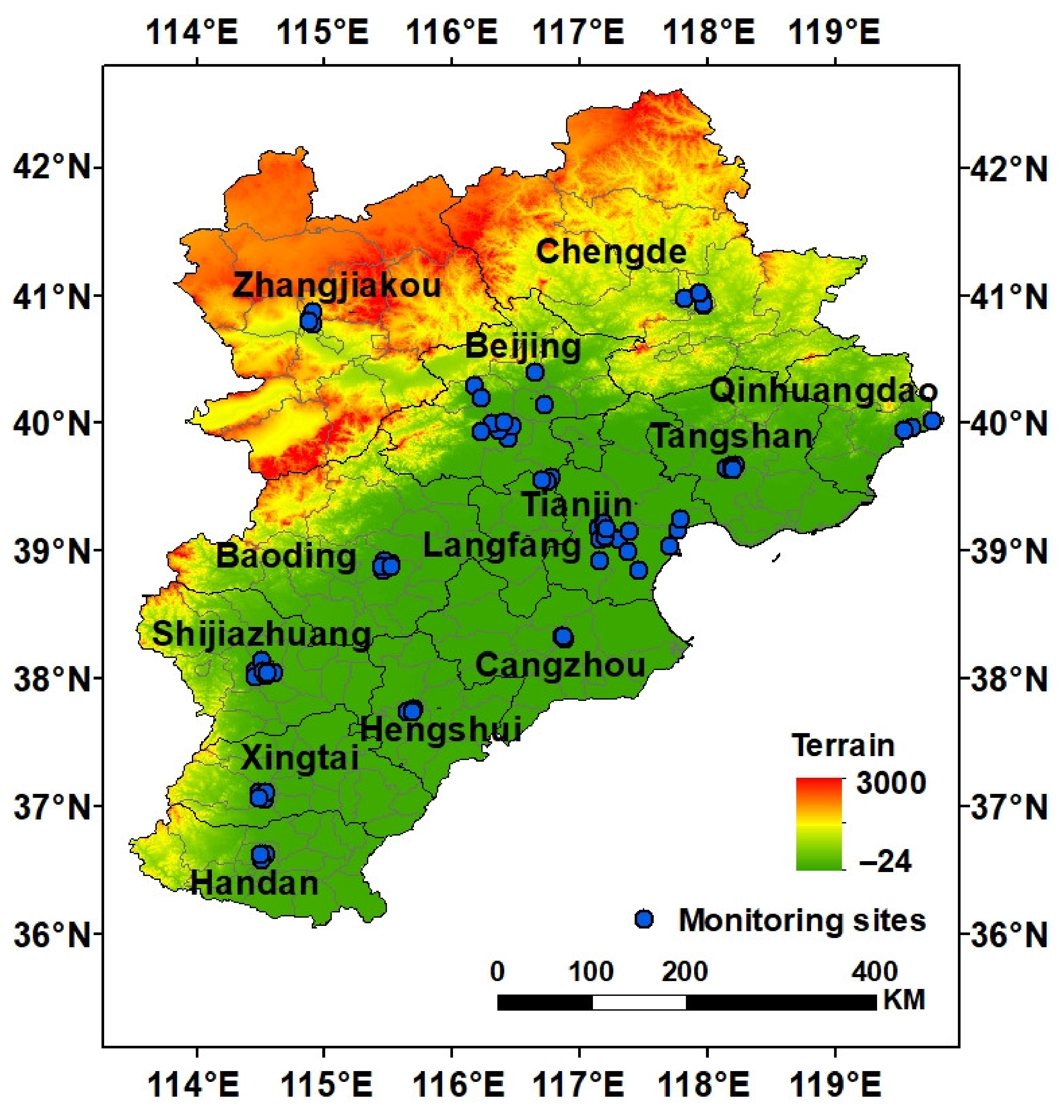
2.1. Study Area

The BTH region, which includes two municipalities (Beijing and Tianjin) and eleven prefecture-level cities in Hebei Province (Figure 1), is one of the three major areas in China characterized by air pollution. Approximately 136 million people live in an area of ~248,000 km2 [29]. Unfortunately, many residents are exposed to high aerosol and O3 loadings. According to the National Urban Air Quality Report in July 2018, most cities in this region, especially those located in the southern BTH region, placed low in the MDA8 O3 ranking among all the cities in China [30].

2.2. Datasets

2.2.1. Near-Surface O3 Monitoring Data

The hourly surface O3 concentration records of 75 monitoring sites in the BTH region were collected from the China Environmental Monitoring Centre (CEMC). The distribution of these sites is shown in Figure 1. To reduce the uncertainty in this dataset, we removed hourly data with less than 8 h of daily monitoring data, and the MDA8 O3 concentration of each station from 1 January 2018, to 31 December 2018, was calculated to construct the model and estimate the near-surface O3 concentration. The O3 dataset used in this study is available at http://113.108.142.147:20035/ (accessed on 25 March 2021).

2.2.2. WRF-Chem Simulation of O3

In this study, the WRF-Chem 3.9.1 was used to simulate the hourly O3 concentration in the BTH region with a spatial resolution of 9 km. WRF-Chem is a fully coupled online atmospheric chemistry model [31] that is generally driven by meteorological and emission data. The meteorological driving datasets were sourced from the National Centers for Environmental Prediction (NCEP) Final Operational Global Analysis with temporal and spatial resolutions of 6 h and 1° × 1°, respectively. The initial field and boundary conditions of the proposed model were built on the basis of these datasets. Emission data are also essential. The emission data were divided into anthropogenic and biogenic emissions. The anthropogenic emission inventory data were obtained from the China Multiresolution Emission Inventory (MEIC) with a 0.25° × 0.25° spatial resolution, and the monthly emission data were converted into hourly emissions. Moreover, the MEIC mainly includes five anthropogenic emission sources, including industrial, power plants, residential, vehicular, and agricultural emissions, and covers 10 major air pollutants and greenhouse gases [32,33,34,35,36]. The biogenic emissions were obtained from the Model of Emissions of Gases and Aerosols from Nature (MEGAN) [37].

2.2.3. Other Auxiliary Data

Meteorological factors can also affect air pollution [38]. Eight meteorological variables were selected to establish the model in this paper: the 2-m temperature (TEM), relative humidity (RH), boundary layer height (BLH), evaporation (ET), surface pressure (SP), wind direction (WD), wind speed (WS), and surface solar radiation downwards (SSRD). All the above parameters were collected from the ERA5 product with spatial and temporal resolutions of 0.25° × 0.25° and 1 h, respectively. In addition, vegetation can also release VOCs; hence, monthly normalized difference vegetation index (NDVI) data collected from the Resource and Environment Data Cloud Platform were also used as input data with a spatial resolution of 1 km. Furthermore, to ensure spatial consistency among the datasets, the spatial resolution of all input data was interpolated to 0.1° × 0.1° by the bilinear interpolation method.

2.3. Methodology

2.3.1. WRFC-XGB Model

In this study, we combined the WRF-Chem model with the XGBoost algorithm to propose a new two-stage method called WRFC-XGB. In the first stage, to map the full-coverage spatial distribution of the surface O3 concentration, we employed the WRF-Chem model to roughly estimate the near-surface MDA8 O3 concentration (SIMO3). The Carbon-Bond Mechanism version Z (CBMZ) was selected for the chemical mechanism because it is more efficient in O3-NO titration than other mechanisms [39,40]. The specific physicochemical parameterization schemes of the WRF-Chem model are shown in Table 1. The model adopts two layers within the nested grid with the coordinate system in a Lambert projection (Figure S1). The resolution of the first layer (D01) is 27 km, and the simulation can cover most of North China while providing the background fields of large-scale atmospheric transport diffusion and pollutant concentrations. In contrast, the resolution of the second layer (D02) is 9 km, and it mainly covers the BTH region. To improve the accuracy of the WRF-Chem model MDA8 O3 simulation, the model was run every month with a spin-up time for the first 168 h.
Then, in the second stage, the XGBoost machine learning model was combined with the SIMO3 obtained in the first stage, meteorological parameters, and NDVI to further calibrate and estimate the MDA8 O3 concentration with full spatiotemporal coverage. The XGBoost model was developed based on gradient enhancement in 2016 [47]. Unlike other machine learning algorithms used in previous studies, each iteration of the XGBoost model adds a tree to fit the residuals between the prediction results of the previous tree, and then the true values are estimated on the basis of the existing tree [48]. In addition, the proposed model incorporates a regularization term, which can effectively prevent overfitting. The model is expressed as the following Equation (1):
O 3 _ P r e i , j = f D O Y i , j ,   T E M i , j , R H i , j , B L H i , j , E T i , j , S P i , j , W D i , j , W S i , j , S S R D i , j , N D V I m , j , S I M O 3   i , j  
where O3_Prei,j indicates the estimated MDA8 O3 concentration on day i at grid j; DOYi,j is the day of year (DOY); TEMi,j, RHi,j, BLHi,j, ETi,j, SPi,j, WDi,j, WSi,j, and SSRDi,j are the values of TEM, RH, BLH, ET, SP, WD, and WS at grid j on day i, respectively; NDVIm,j is the NDVI value in month m at grid j; and SIMO3i,j denotes the WRF-Chem model output of the MDA8 O3 concentration on day i at grid j. Similar to the inverse distance weighting (IDW) [49], the DOY was used the weighted time distance, namely, the reciprocal of the distance from each day to the middle of the year, which can better reflect the continuity of the daily variation in O3 pollution. Before constructing the model, we conducted a correlation analysis for all independent variables (Table 2); the results show that all correlations were statistically significant (p < 0.01). Among them, a positive relationship was captured between the O3 concentration and TEM, RH, BLH, WD, WS, SSRD, NDVI, and SIMO3, while a negative relationship was found with ET and SP. In addition, to avoid the systematic errors caused by multicollinearity, the variance inflation factor (VIF) index was calculated to identify the collinearity among all independent variables used in the WRFC-XGB model. A VIF smaller than 10 indicates the absence of multicollinearity in our model. According to the results, no multicollinearity existed in our model (VIF < 10). Furthermore, we compared the WRFC-XGB model with other machine learning methods (Table S1).
To further evaluate the WRFC-XGB model, the traditional models used previous studies to estimate the O3 concentration were selected for comparison: the MLR model, generalized additive model (GAM), GWR model, and linear mixed effect (LME) model [22,50,51,52]. The same training dataset was used for each of these four models for the O3 estimation in 2018.

2.3.2. Evaluation Method

To test the estimation performance of the WRFC-XGB model, the commonly used 10-CV method was applied herein. For this method, the observation results were first randomly divided into ten parts. Then, nine subsets were selected as the training data, and another subset was used as the verification data. The above process was repeated 10 times to ensure that each dataset was verified once, and the average values of 10 verification results were taken as the final result [53]. Furthermore, according to the division of subsets for 10-CV, we employed sample-based 10-CV and station-based 10-CV to evaluate the model [54]. In addition, four indexes, namely, the regression line, R2, root mean square error (RMSE), and mean absolute error (MAE), between the observed and estimated O3 were also calculated to evaluate the agreement between the simulated results and measurements.

3. Results and Discussion

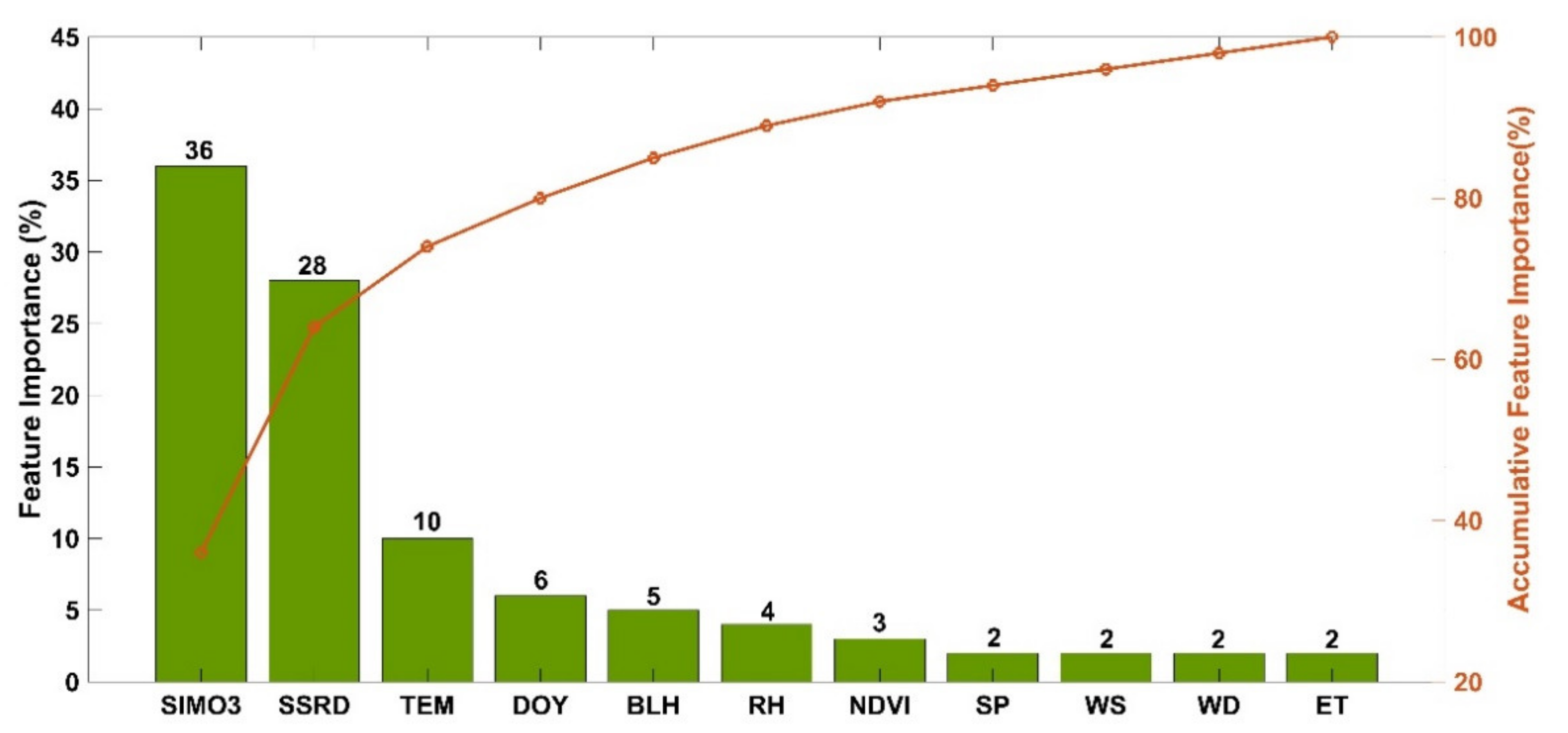
3.1. Feature Importance

Before estimating the MDA8 O3 concentrations, the applicability of independent variables was evaluated first. Figure 2 shows the feature importance (FI) of all input variables of the WRFC-XGB model. For this figure, the FI indicates the contribution of each independent variable to the established model, and the maximum FI is 100%, where a higher FI indicates a greater impact of the input variable on the MDA8 O3 estimation. In general, the highest contribution was captured in SIMO3 with an FI of 36%, which can clarify the rationality of our model and the accuracy of the WRF-Chem simulation, followed by SSRD with an FI of 28%. As a general rule, radiation is conducive to photochemical reactions, resulting in the formation of O3, and heavy O3 pollution episodes are usually accompanied by high levels of radiation or severe weather conditions with more precursors [10]. Another important reaction condition is temperature, which accounts for 10% of the MDA8 O3 estimation. Temperature is one of the main driving factors responsible for generating O3. On the one hand, temperature can affect O3 concentrations by influencing atmospheric turbulence and photochemical reactions [55,56]. On the other hand, temperature can increase the biological emission of VOCs, thus increasing the O3 concentration in the BTH region [57]. Following these variables, the total contribution of all the other meteorological factors, including BLH, RH, SP, WD, WS, and ET, was ~17%, indicating that these variables affect the generation, transmission, and dissipation of O3 to varying degrees [58,59,60,61]. Notably, the FI of DOY was approximately 6%, indicating that the surface O3 concentration exhibited a significant temporal variation that could be captured effectively by our WRFC-XGB model.

3.2. Model Accuracy Evaluation

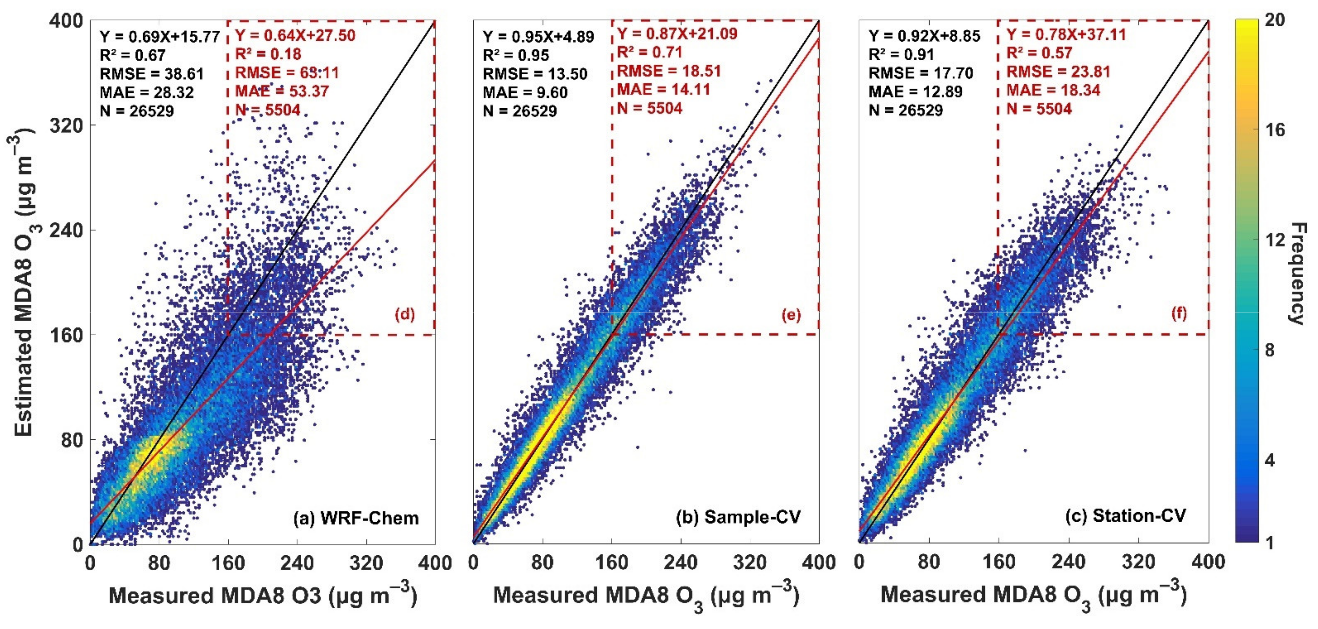
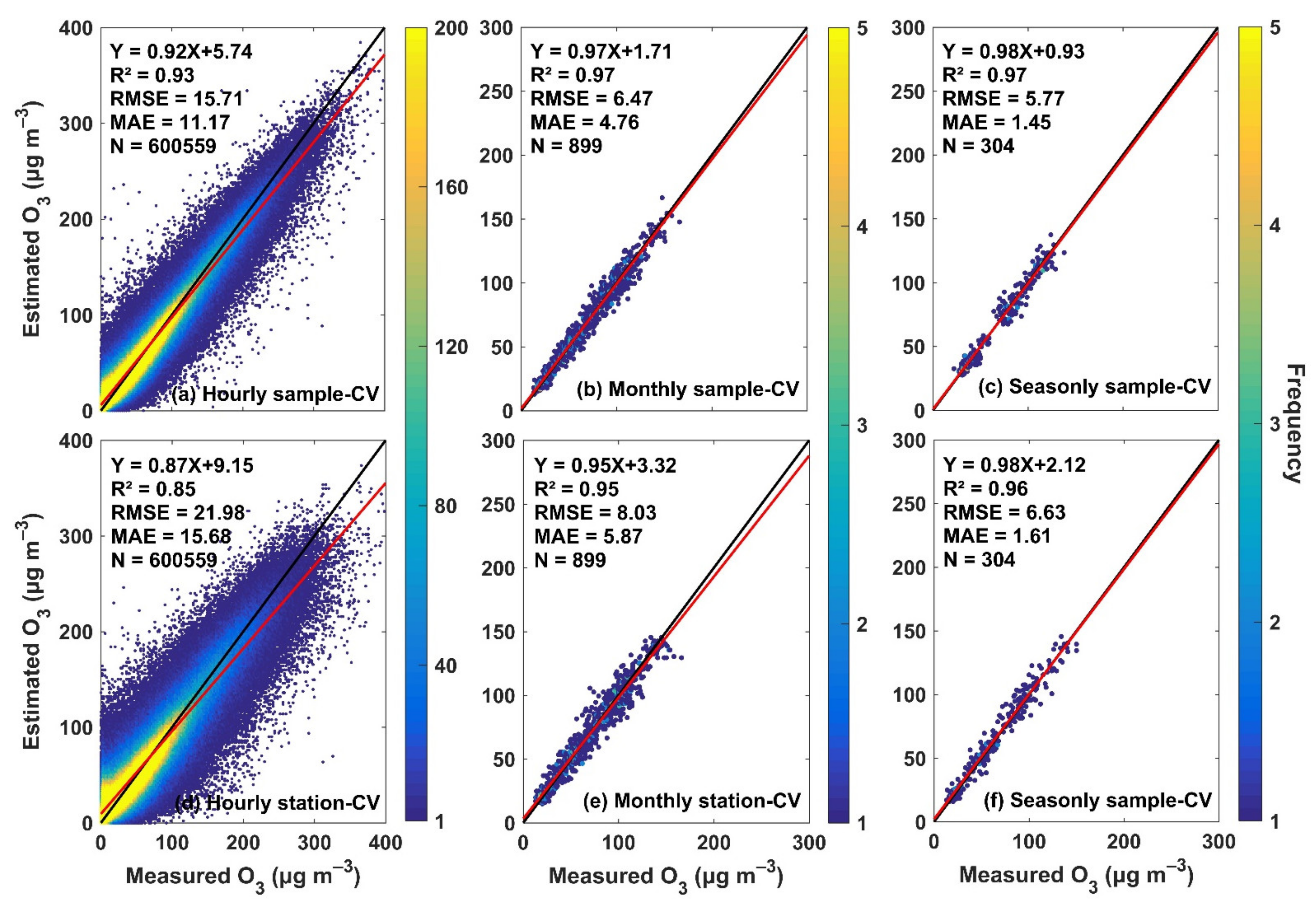
3.2.1. Overall Accuracy

Figure 3 shows both the validation results of the WRF-Chem model simulation and the 10-CV results of the WRFC-XGB model. In general, the simulated MDA8 O3 concentrations of the WRFC-Chem model are low (Figure 3a), with a low R2 of 0.67, and the RMSE and MAE of the WRF-Chem model simulation are high at 38.61 µg m−3 and 28.32 µg m−3, respectively. Compared with the WRF-Chem validation results, the estimation accuracies of the XGBoost machine learning method are greatly improved for both the sample-based and the station-based 10-CV, with the R2 increasing by 0.28 and 0.24, respectively, and the RMSE (MAE) decreases by 25.11 µg m−3 (18.72 µg m−3) and 20.91 µg m−3 (15.43 µg m−3), respectively. However, the values estimated by the WRFC-XGB model are slightly underestimated, mainly due to the values simulated by WRF-Chem being far lower than the observed concentrations. However, the scattered points are concentrated mainly near the 1:1 line, showing no serious deviation overall.
Furthermore, to explore the simulation results in periods with high O3 pollution, we examined the predictive ability of the WRFC-XGB model for MDA8 O3 concentrations exceeding the Class 2 Chinese Ambient Air Quality Standard (>160 µg m−3). The WRF-Chem model-simulated MDA8 O3 concentrations exhibit great uncertainty with an extremely low R2 of only 0.18, and the RMSE and MAE reach 63.11 µg m−3 and 53.37 µg m−3, respectively. These large errors generated by the WRF-Chem model may be due to the lag of the emission inventory and the uncertainties in the meteorological factors such WS and BLH. Compared with the WRF-Chem model, the WRFC-XGB model can effectively improve the MDA8 O3 estimation accuracy of during heavy O3 pollution periods, with the sample-based 10-CV R2 approximately tripling (R2 = 0.71) compared with the WRF-Chem model alone. The station-based 10-CV estimation accuracy is also improved (R2 = 0.57). This significant improvement in the estimation accuracy is due to the excellent autonomous learning and expression capabilities of the XGBoost machine learning method, which effectively corrects the errors of the WRF-Chem model. Overall, our WRFC-XGB model can effectively and precisely estimate the MDA8 O3 concentrations across the BTH region not only during periods of light pollution but also during periods of heavy pollution.

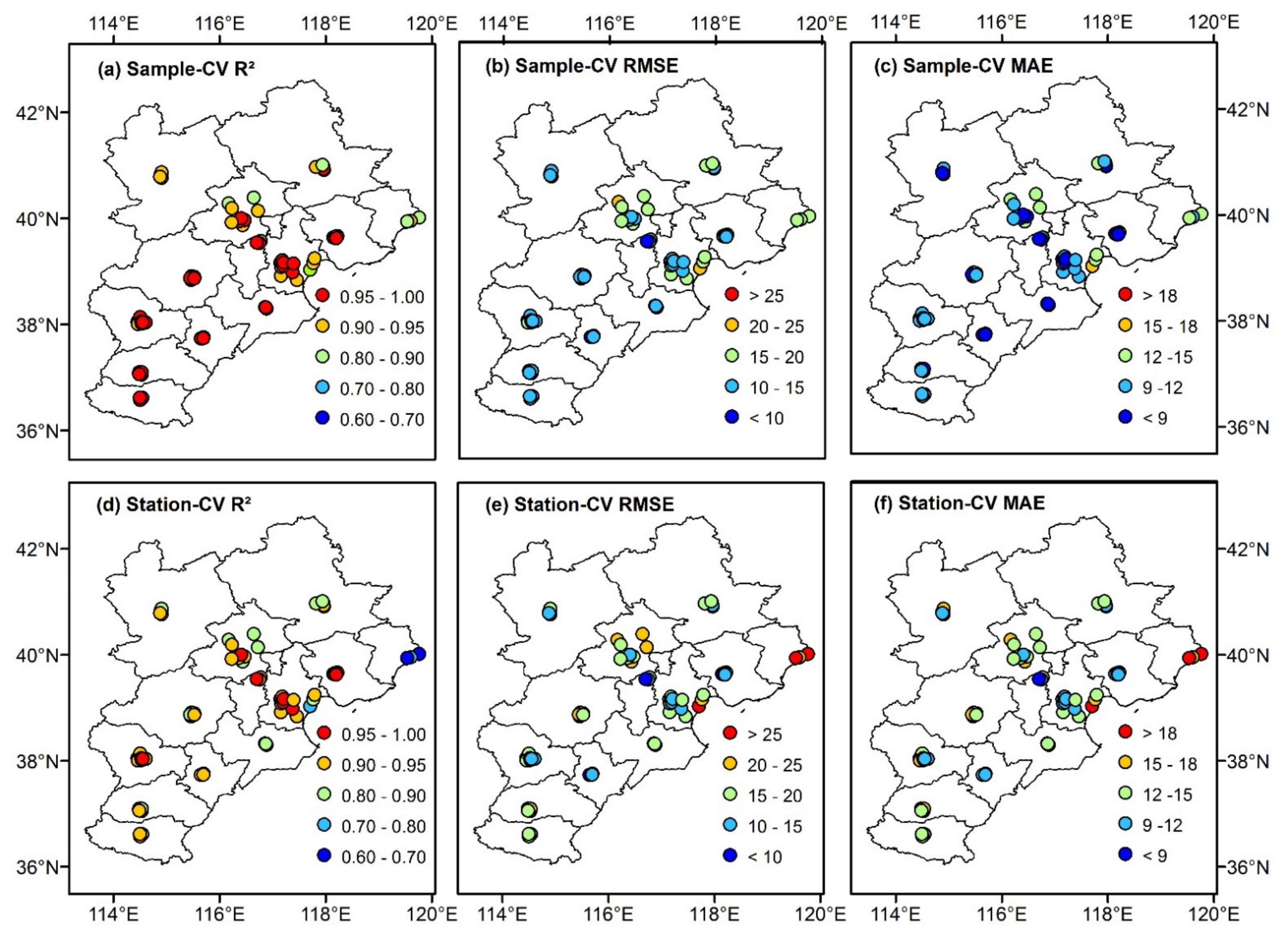
3.2.2. Spatial Consistency Verification

The O3 concentrations show significant spatial heterogeneity across the BTH region, which could also cause uncertainty in the spatial MDA8 O3 concentration distribution at different scales. Therefore, we calculated the three evaluation indicators for sample-based and station-based 10-CV at each station in the BTH region. Figure 4 plots the spatial distributions of the R2, RMSE, and MAE at each surface measurement site in the BTH region in 2018 from the sample- and station-based 10-CV for our WRFC-XGB model. In general, our WRFC-XGB model yields superb spatial O3 estimates. For the sample-based 10-CV, the highest R2 is 0.98, which is found in Langfang. All sites exhibit an R2 greater than 0.85, 97% of all sites have an RMSE less than 20 µg m−3, and 99% of all sites hold an MAE less than 15 µg m−3 (Figure S2). In contrast, the lowest R2 is 0.86 in Tianjin, and the site is near the Bohai Sea. The accuracies at the sites located in Qinhuangdao near the Bohai Sea are also relatively low, similar to the spatial distribution simulated by the WRF-Chem model (Figure S3). This may be because these stations are affected by the sea breeze, and the WD and WS simulated by the WRF-Chem model have large errors relative to the other meteorological elements. For the station-based 10-CV, the R2 is greater than 0.85 at 91% of the sites, the RMSE is less than 20 µg m−3 at 79% of the sites, and the MAE is less than 15 µg m−3 at 79% of the sites. Overall, the simulation results of the WRFC-XGB model display good spatial heterogeneity and can capture the characteristics in both high- and low-pollution areas, which can be used to analyze and interpret the spatial differences in the O3 concentration.

3.2.3. Temporal Consistency Verification

Figure 5 shows the frequency density scatter plots for the sample-based and station-based 10-CV results of O3 concentration estimation at hourly, monthly, and seasonal scales, respectively. Among all, the worst-performing was captured at hourly scale, with a sample-based (station-based) 10-CV R2 of 0.93 (0.85), RMSE of 15.71 µg m−3 (21.98 µg m−3), and MAE of 11.17 µg m−3 (15.68 µg m−3), respectively. Moreover, the R2, RMSE, and MAE of sample-based 10-CV at monthly scale is 0.97, 6.47 µg m−3, and 4.76 µg m−3, respectively, while those indexes for the station-based 10-CV is 0.95, 8.03 µg m−3, and 5.87 µg m−3, respectively. More important, the R2, RMSE, and MAE values of the seasonal sample-based (station-based) 10-CV are 0.97 (0.96), 5.77 µg m−3 (6.63 µg m−3), and 1.45 µg m−3 (1.61 µg m−3), respectively. Overall, the WRFC-XGB model shows a strong estimation ability on all time scales, and the accuracy of our model increases as the time scale lengthens because the model needs to capture fewer characteristic features. In addition, the accuracy of sample-based 10-CV is higher than that of station-based 10-CV at all time scales, which is consistent with another previous study [62], mainly because the O3 concentration characteristics between similar sites are more similar than those between distant sites, and station-based 10-CV reduce the number of sites for the training data.

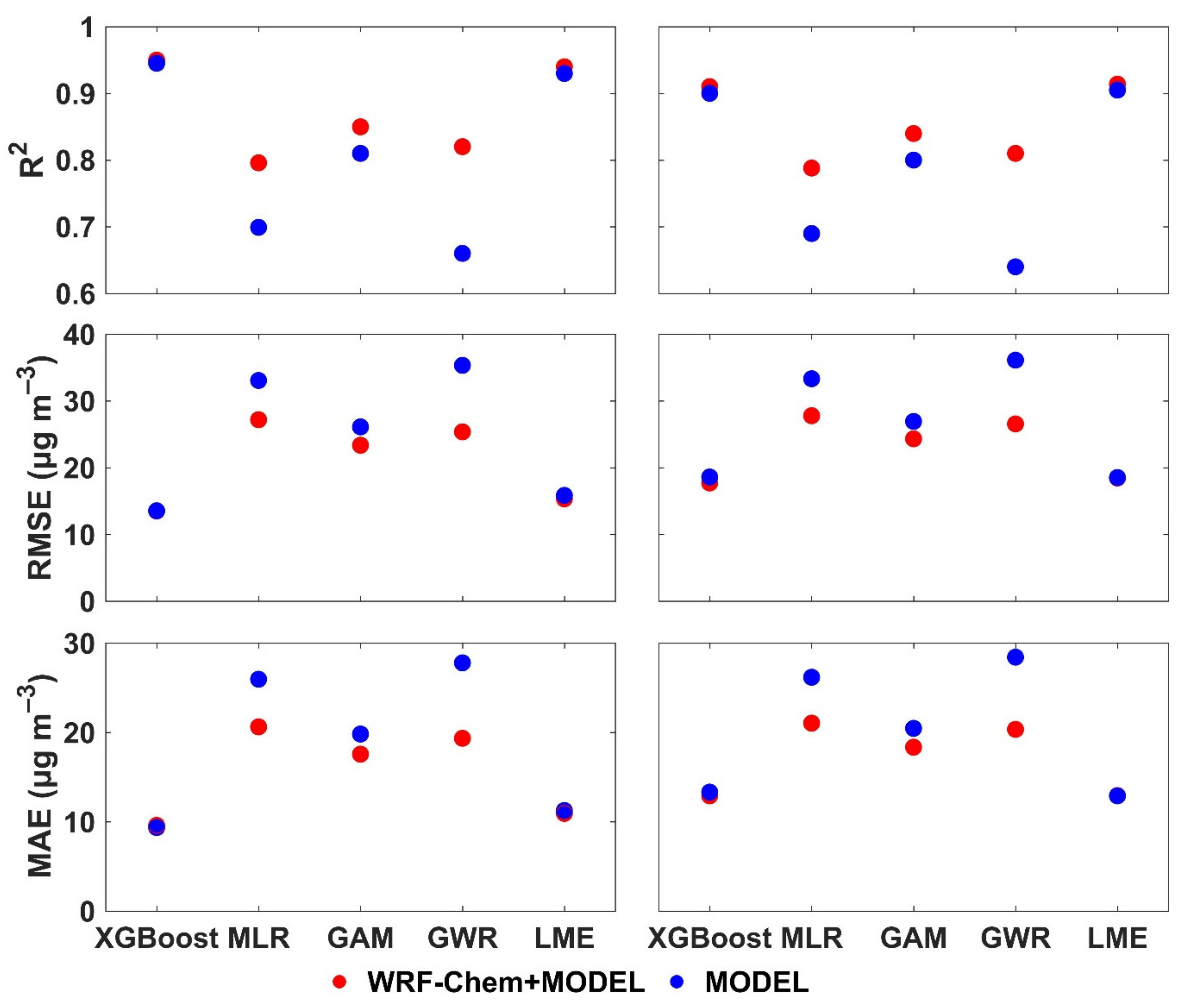
3.3. Comparison with Other Traditional Models and Studies

Figure 6 presents a comparison of the MDA8 O3 estimation accuracy between the XGBoost method and four traditional models (MLR, GAM, GWR, and LME). Using the SIMO3 obtained in the WRF-Chem model for the model establishment, the R2 range of all models is 0.64–0.95. The model with the worst accuracy is MLR, with a sample-based (station-based) 10-CV R2 of 0.80 (0.79) and corresponding RMSE and MAE values of 27.20 µg m−3 (27.79 µg m−3) and 20.63 µg m−3 (21.05 µg m−3), respectively. This is mainly because MLR considers only simple linear relationships between the O3 concentration and input variables. However, GAM adopts nonlinear regression, and its estimation accuracy is improved compared with that of MLR, with a sample-based (station-based) 10-CV R2 of 0.85 (0.84), RMSE of 23.38 µg m−3 (24.33 µg m−3), and MAE of 17.58 µg m−3 (18.35 µg m−3). Furthermore, the sample-based (station-based) 10-CV R2 of GWR is 0.82 (0.81), while its RMSE and MAE are 25.36 µg m−3 (26.56 µg m−3) and 19.35 µg m−3 (20.34 µg m−3), respectively. The estimation accuracy of the LME model is the highest among these traditional models and is even close to that of the WRFC-XGB model. Its sample-based (station-based) 10-CV R2 is 0.94 (0.91), and its RMSE and MAE are 15.32 µg m−3 (18.44 µg m−3) and 10.94 µg m−3 (12.93 µg m−3), respectively. This is mainly because the LME model considers both fixed effects and random effects. Fixed effects represent the annual average state of influence of each input variable on O3, while random effects are used to explain the diurnal variation relationships between O3 and SIMO3 and the meteorological factors, as well as the monthly variation relationship between O3 and NDVI. Nevertheless, although the estimation accuracy of the LME model is similar to that of the WRFC-XGB model, it requires an excessively long computation time and a large number of calculations.
Moreover, without using SIMO3 as an input variable, the estimation accuracies of these traditional models are reduced for both sample-based and station-based 10-CV (Figure S4). The results indicate that the SIMO3 dataset obtained by the WRF-Chem model plays a vital role in improving the O3 estimation accuracy. In addition, the worst-performing model at this time is not MLR but GWR, mainly because GWR is a spatial analysis algorithm that is based on the local effects of objects distributed in space, and thus, considers the influences of spatial changes in the model input variables on the estimated O3 concentration [63]. In the WRF-Chem model, although the simulated O3 concentration is low overall, its spatial distribution is reasonable, and therefore, provides a good basis for estimating the O3 for GWR. Therefore, after removing the O3 concentration output from the WRF-Chem model, the estimation accuracy of GWR drops the most below even that of MLR.
To further prove the reliability of the WRFC-XGB model proposed in this study, we compared the results of our model with the conclusions of existing publications (Table 3), including the results of sample-based and station-based verification analyses. Taking the sample-based verification results as an example, the nationwide O3 estimation accuracies based on the data fusion model (5-CV R2 = 0.7, RMSE = 26 µg m−3) [64] and the RF (10-CV R2 = 0.69, RMSE = 26 µg m−3) and XGBoost models (10-CV R2 = 0.78, RMSE = 21.47 µg m−3) are all lower than that of our model [23,62]. In addition, some studies have estimated the O3 concentrations in other regions. For instance, Li et al. [65,66] estimated the O3 concentrations on Hainan Island (10-CV R2 = 0.59) and the Qinghai-Tibet Plateau (10-CV R2 = 0.76, RMSE = 14.41 µg m−3). Compared with the application of other models on the same spatial (regional) scale (10-CV R2 = 0.84) [67], our model achieves a higher estimation accuracy. This is mainly because the result of a high-resolution (9 km × 9 km) model with physicochemical principles (WRF-Chem) is incorporated into the WRFC-XGB model, which reduces the deviation caused by interpolation.

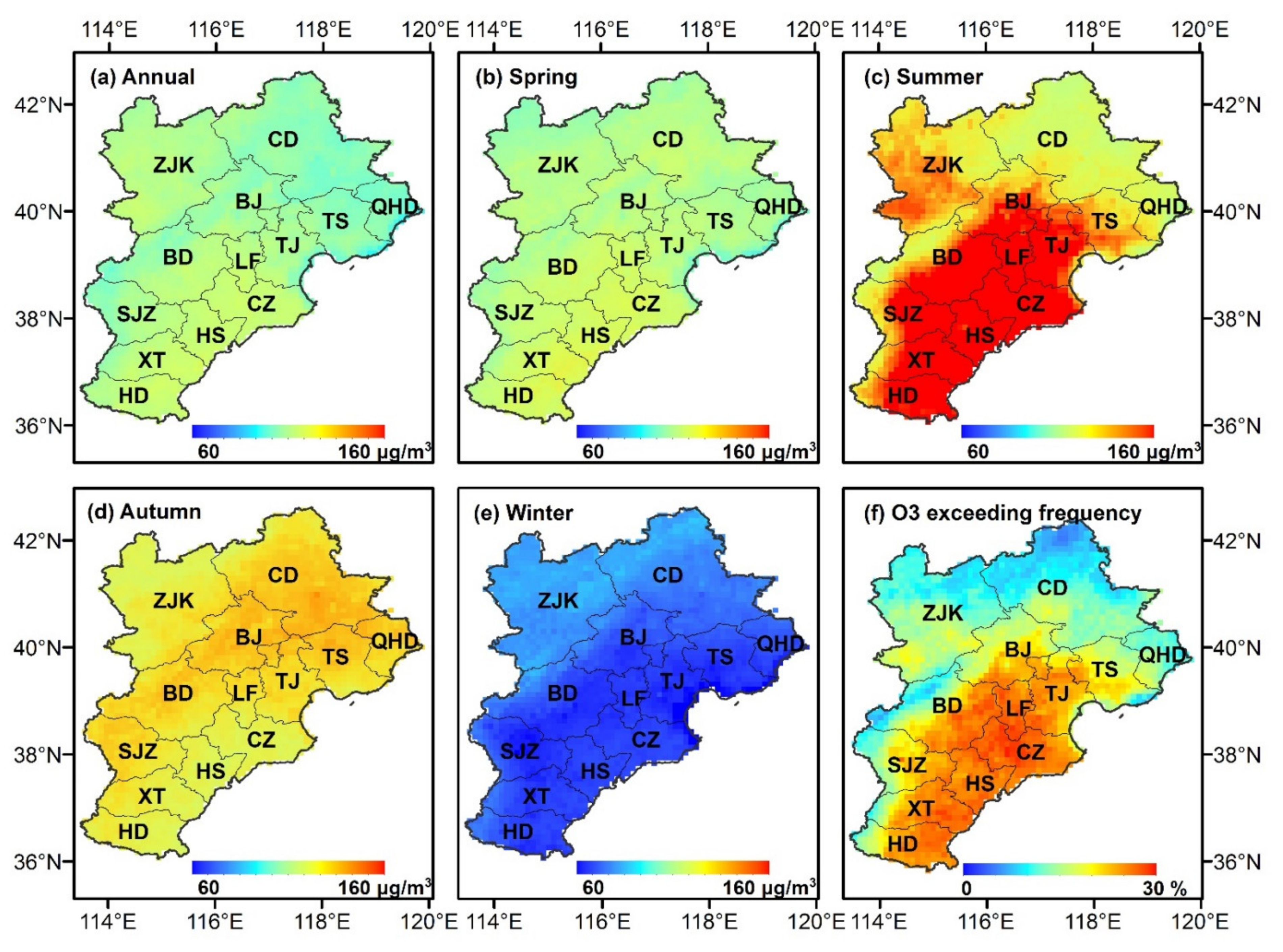
3.4. Spatial Distribution of MDA8 O3 in the BTH Region

The distribution of observation sites in the BTH region is uneven; most of the sites are located in Beijing and Tianjin, and some of them lack measurements. In general, the MDA8 O3 concentration at all sites in the BTH region in 2018 was 106.67 ± 60.29 µg m−3. In this study, the WRFC-XGB model was used to estimate the spatial and temporal coverage of the MDA8 O3 concentration with a spatial resolution of 0.1° × 0.1° in the BTH region in 2018. Figure 6b–e shows the concentrations of MDA8 O3 estimated by WRFC-XGB in the spring, summer, autumn, and winter in the BTH region. The results demonstrate that the spatial distribution of the MDA8 O3 concentration exhibits obvious seasonality. The concentrations of MDA8 O3 in spring, summer, autumn, and winter were 100.93–145.74 µg m−3, 123.05–194.42 µg m−3, 61.13–94.60 µg m−3, and 44.22–82.74 µg m−3, respectively. As expected, the O3 concentration in summer is much higher than that in the other seasons due to the long sunshine duration, strong solar radiation, and active photochemical reactions in summer, all of which are conducive to the formation of high concentrations of O3 [68]. Moreover, high temperatures lead to significant increases in the VOC emissions of O3 precursors, especially from natural sources, resulting in serious O3 pollution [69].
According to the results of the WRFC-XGB model, there are obvious spatial differences in the estimated MDA8 O3 concentration, with higher O3 concentrations in Beijing, Tianjin, and southern Hebei, which is consistent with the results of Xue et al. [64]. Figure 7f shows the spatial distribution of the frequency of O3 concentrations exceeding the standard (the percentage of days when the O3 concentration exceeds the standard divided by 365), yielding values between 5% and 30%, which is similar to the summertime distribution of the MDA8 O3 concentration (Figure 7c). O3 is known to have a complicated nonlinear relationship with VOC precursors and NOx (NO + NO2 = NOX). In China, power plants, industry, and transportation are the main sources of NOX emissions, accounting for approximately 88% of total NOX emissions [70]. The population distribution of the BTH region varies considerably, where the population is most densely concentrated in Beijing, Tianjin, and the central and southern regions of Hebei [71]. These densely populated areas have large traffic flows and developed industries, and thus, are characterized by the highest emissions in the BTH region. A previous study showed that Beijing, Tianjin, Shijiazhuang, Tangshan, and Handan account for 65.4% and 65.2% of the total NOx and CO emissions of BTH, respectively [72]. In addition to anthropogenic emissions, topography also has a significant impact on O3 pollution. The BTH region is composed mainly of the Bashang Plateau, Taihang Mountains, Yanshan Mountains, and northern part of the North China Plain. Because the study area is topographically surrounded by mountains, southeasterly winds can blow pollutants toward Beijing and accumulate; hence, Beijing is prone to heavy pollution incidents [73].

4. Conclusions

Since 2013, many O3 concentration measurement sites have been built in China. However, the spatial distribution of those sites is uneven, resulting in an inadequate understanding of the surface O3 loading, especially in the BTH region. Therefore, a new method, i.e., the WRFC-XGB model, which combines the WRF-Chem model with the XGBoost machine learning algorithm, was developed in this study. Combining SIMO3 data, meteorological data, NDVI data, and DEM data, the MDA8 O3 concentration across the BTH region in 2018 was estimated based on this model. Compared with the results of previous studies and other traditional methods, our model shows higher accuracy and better spatial prediction capabilities, with sample-based and station-based 10-CV R2 (RMSE) values of 0.95 (13.50 µg m−3) and 0.91 (17.70 µg m−3), respectively. Then, we employed the WRFC-XGB model to estimate the full spatiotemporal coverage of MDA8 O3 in the BTH region. The results show that the MDA8 O3 concentration is 106.67 ± 60.29 µg m−3 in BTH. The O3 concentration has obvious spatial differences across BTH, with high O3 concentrations being found in Beijing, Tianjin, and southern Hebei. Overall, our WRFC-XGB method possesses superior O3 estimation performance; thus, it can be widely used for estimating O3 over long-term and wide spatial scales.

Supplementary Materials

The following supporting information can be downloaded at: https://www.mdpi.com/article/10.3390/atmos13040632/s1, Figure S1: Double-layer nesting distribution in the WRF-Chem model, the color bar represents the altitude; Figure S2: Probability density functions (PDFs) and cumulative density functions (CDFs) of the sample-based (red columns) and station-based (blue columns) 10-fold cross-validation; Figure S3: The validation results of the WRF-Chem simulations and site observations in the Beijing-Tian-Hebei region in 2018; Figure S4: The scatter density plot of the final estimation accuracy of different traditional models with and without fusion of the WRF-Chem model; Table S1: Comparison of MDA8 O3 concentration estimation accuracy between integrating different machine learning algorithms with the WRF-Chem model and the WRFC-XGB model.

Author Contributions

Conceptualization, X.H.; methodology, X.H.; software, X.H.; validation, X.H.; validation, W.X.; formal analysis, X.H.; data curation, Y.C. and T.H.; writing—original draft preparation, X.H.; writing—review and editing, J.Z., W.X. and L.Z.; funding acquisition, J.Z. All authors have read and agreed to the published version of the manuscript.

Funding

This study was supported by the National Natural Science Foundation of China (41575144), the National Key R&D Program of China (2017YFA0603603), and the BNU Interdisciplinary Research Foundation for the First-Year Doctoral Candidates (BNUXKJC2026).

Institutional Review Board Statement

Not applicable.

Informed Consent Statement

Not applicable.

Data Availability Statement

The ERA5 data are available at https://www.ecmwf.int/en/forecasts/datasets/reanalysis-datasets/era5 (accessed on 25 March 2021). The NDVI data are available at https://www.resdc.cn/data.aspx?DATAID=254 (accessed on 2 April 2021).

Conflicts of Interest

The authors declare no conflict of interest.

References

  1. U.S. Environmental Protection Agency. Integrated Science Assessment for Ozone and Related Photochemical Oxidants; U.S. Environmental Protection Agency: Washington, DC, USA, 2013.
  2. Jerrett, M.; Burnett, R.T.; Pope, C.A., III; Ito, K.; Thurston, G.; Krewski, D.; Shi, Y.; Calle, E.; Thun, M. Long-Term Ozone Exposure and Mortality. N. Engl. J. Med. 2009, 360, 1085–1095. [Google Scholar] [CrossRef] [PubMed] [Green Version]
  3. Sitch, S.; Cox, P.; Collins, W.; Huntingford, C. Indirect radiative forcing of climate change through ozone effects on the land-carbon sink. Nature 2007, 448, 791–794. [Google Scholar] [CrossRef] [PubMed]
  4. Fu, Y.; Liao, H.; Yang, Y. Interannual and Decadal Changes in Tropospheric Ozone in China and the Associated Chemistry-Climate Interactions: A Review. Adv. Atmos. Sci. 2019, 36, 975–993. [Google Scholar] [CrossRef]
  5. Wang, T.; Xue, L.; Brimblecombe, P.; Lam, Y.F.; Li, L.; Zhang, L. Ozone pollution in China: A review of concentrations, meteorological influences, chemical precursors, and effects. Sci. Total Environ. 2016, 575, 1582–1596. [Google Scholar] [CrossRef]
  6. Liang, S.; Li, X.; Teng, Y.; Fu, H.; Chen, L.; Mao, J.; Zhang, H.; Gao, S.; Sun, Y.; Ma, Z.; et al. Estimation of health and economic benefits based on ozone exposure level with high spatial-temporal resolution by fusing satellite and station observations. Environ. Pollut. 2019, 255, 113267. [Google Scholar] [CrossRef]
  7. Qu, L.; Liu, S.; Ma, L.; Zhang, Z.; Du, J.; Zhou, Y.; Meng, F. Evaluating the meteorological normalized PM2.5 trend (2014–2019) in the “2+26” region of China using an ensemble learning technique. Environ. Pollut. 2020, 266, 115346. [Google Scholar] [CrossRef]
  8. Zheng, B.; Tong, D.; Li, M.; Liu, F.; Hong, C.; Geng, G.; Li, H.; Li, X.; Peng, L.; Qi, J.; et al. Trends in China’s anthropogenic emissions since 2010 as the consequence of clean air actions. Atmos. Chem. Phys. 2018, 18, 14095–14111. [Google Scholar] [CrossRef] [Green Version]
  9. Xiang, S.; Liu, J.; Tao, W.; Yi, K.; Xu, J.; Hu, X.; Liu, H.; Wang, Y.; Zhang, Y.; Yang, H.; et al. Control of both PM2.5 and O3 in Beijing-Tianjin-Hebei and the surrounding areas. Atmos. Environ. 2020, 224, 117259. [Google Scholar] [CrossRef]
  10. Gao, D.; Xie, M.; Chen, X.; Wang, T.; Zhan, C.; Ren, J.; Liu, Q. Modeling the Effects of Climate Change on Surface Ozone during Summer in the Yangtze River Delta Region, China. Int. J. Environ. Res. Public Heal. 2019, 16, 1528. [Google Scholar] [CrossRef] [Green Version]
  11. Li, K.; Jacob, D.J.; Liao, H.; Shen, L.; Zhang, Q.; Bates, K.H. Anthropogenic drivers of 2013–2017 trends in summer surface ozone in China. Proc. Natl. Acad. Sci. USA 2018, 116, 422–427. [Google Scholar] [CrossRef] [Green Version]
  12. Zhang, L.; Jacob, D.J.; Downey, N.V.; Wood, D.A.; Blewitt, D.; Carouge, C.C.; van Donkelaar, A.; Jones, D.B.; Murray, L.; Wang, Y. Improved estimate of the policy-relevant background ozone in the United States using the GEOS-Chem global model with 1/2° × 2/3° horizontal resolution over North America. Atmos. Environ. 2011, 45, 6769–6776. [Google Scholar] [CrossRef] [Green Version]
  13. Mathur, R.; Xing, J.; Napelenok, S.; Pleim, J.; Hogrefe, C.; Wong, D.; Gan, C.-M.; Kang, D. Multiscale Modeling of Multi-decadal Trends in Ozone and Precursor Species Across the Northern Hemisphere and the United States. In Air Pollution Modeling and its Application XXIV; Springer: Berlin/Heidelberg, Germany, 2016; pp. 239–243. [Google Scholar] [CrossRef]
  14. Lu, X.; Zhang, L.; Chen, Y.; Zhou, M.; Zheng, B.; Li, K.; Liu, Y.; Lin, J.; Fu, T.-M.; Zhang, Q. Exploring 2016–2017 surface ozone pollution over China: Source contributions and meteorological influences. Atmos. Chem. Phys. 2019, 19, 8339–8361. [Google Scholar] [CrossRef] [Green Version]
  15. Qiao, X.; Guo, H.; Wang, P.; Tang, Y.; Ying, Q.; Zhao, X.; Deng, W.; Zhang, H. Fine Particulate Matter and Ozone Pollution in the 18 Cities of the Sichuan Basin in Southwestern China: Model Performance and Characteristics. Aerosol Air Qual. Res. 2019, 19, 2308–2319. [Google Scholar] [CrossRef] [Green Version]
  16. Adam-Poupart, A.; Brand, A.; Fournier, M.; Jerrett, M.; Smargiassi, A. Spatiotemporal Modeling of Ozone Levels in Quebec (Canada): A Comparison of Kriging, Land-Use Regression (LUR), and Combined Bayesian Maximum Entropy–LUR Approaches. Environ. Heal. Perspect. 2014, 122, 970–976. [Google Scholar] [CrossRef]
  17. Lefohn, A.S.; Knudsen, H.; McEvoy, L.R. The use of kriging to estimate monthly ozone exposure parameters for the Southeastern United States. Environ. Pollut. 1988, 53, 27–42. [Google Scholar] [CrossRef]
  18. Li, L. An Application of a Shape Function Based Spatiotemporal Interpolation Method to Ozone and Population-Based Environmental Exposure in the Contiguous U.S. J. Environ. Inform. 2008, 12, 120–128. [Google Scholar] [CrossRef]
  19. Ghazali, N.A.; Ramli, N.A.; Yahaya, A.S.; Yusof, N.F.F.M.; Sansuddin, N.; Al Madhoun, W.A. Transformation of nitrogen dioxide into ozone and prediction of ozone concentrations using multiple linear regression techniques. Environ. Monit. Assess. 2009, 165, 475–489. [Google Scholar] [CrossRef]
  20. Sousa, S.; Martins, F.; Alvimferraz, M.; Pereira, M. Multiple linear regression and artificial neural networks based on principal components to predict ozone concentrations. Environ. Model. Softw. 2007, 22, 97–103. [Google Scholar] [CrossRef]
  21. Alvarez-Mendoza, C.I.; Teodoro, A.; Cando, L.R. Spatial estimation of surface ozone concentrations in Quito Ecuador with remote sensing data, air pollution measurements and meteorological variables. Environ. Monit. Assess. 2019, 191, 155. [Google Scholar] [CrossRef]
  22. Zhang, X.Y.; Zhao, L.M.; Cheng, M.M.; Chen, D.M. Estimating Ground-Level Ozone Concentrations in Eastern China Using Satellite-Based Precursors. IEEE Trans. Geosci. Remote Sens. 2020, 58, 4754–4763. [Google Scholar] [CrossRef]
  23. Zhan, Y.; Luo, Y.Z.; Deng, X.F.; Grieneisen, M.L.; Zhang, M.H.; Di, B.F. Spatiotemporal prediction of daily ambient ozone levels across China using random forest for human exposure assessment. Environ. Pollut. 2018, 233, 464–473. [Google Scholar] [CrossRef] [PubMed]
  24. Chen, G.; Chen, J.; Dong, G.-H.; Yang, B.-Y.; Liu, Y.; Lu, T.; Yu, P.; Guo, Y.; Li, S. Improving satellite-based estimation of surface ozone across China during 2008–2019 using iterative random forest model and high-resolution grid meteorological data. Sustain. Cities Soc. 2021, 69, 102807. [Google Scholar] [CrossRef]
  25. Xue, W.; Zhang, J.; Zhong, C.; Li, X.; Wei, J. Spatiotemporal PM2.5 variations and its response to the industrial structure from 2000 to 2018 in the Beijing-Tianjin-Hebei region. J. Clean. Prod. 2020, 279, 123742. [Google Scholar] [CrossRef]
  26. Wei, J.; Li, Z.; Xue, W.; Sun, L.; Fan, T.; Liu, L.; Su, T.; Cribb, M. The ChinaHighPM10 dataset: Generation, validation, and spatiotemporal variations from 2015 to 2019 across China. Environ. Int. 2020, 146, 106290. [Google Scholar] [CrossRef]
  27. Li, T.; Wang, Y.; Yuan, Q. Remote Sensing Estimation of Regional NO2 via Space-Time Neural Networks. Remote Sens. 2020, 12, 2514. [Google Scholar] [CrossRef]
  28. Geng, G.; Xiao, Q.; Liu, S.; Liu, X.; Cheng, J.; Zheng, Y.; Xue, T.; Tong, D.; Zheng, B.; Peng, Y.; et al. Tracking Air Pollution in China: Near Real-Time PM2.5 Retrievals from Multisource Data Fusion. Environ. Sci. Technol. 2021, 55, 12106–12115. [Google Scholar] [CrossRef]
  29. Guo, X.; Fu, L.; Ji, M.; Lang, J.; Chen, D.; Cheng, S. Scenario analysis to vehicular emission reduction in Beijing-Tianjin-Hebei (BTH) region, China. Environ. Pollut. 2016, 216, 470–479. [Google Scholar] [CrossRef]
  30. Ministry of Ecology and Environmental of the People’s Republic of China (MEE). National Urban Air Quality Status in 2018. 2018. Available online: http://www.mee.gov.cn/hjzl/dqhj/cskqzlzkyb/201809/P020180905326235405574.pdf (accessed on 4 March 2021).
  31. Grell, G.A.; Peckham, S.E.; Schmitz, R.; McKeen, S.A.; Frost, G.; Skamarock, W.C.; Eder, B. Fully coupled “online” chemistry within the WRF model. Atmos. Environ. 2005, 39, 6957–6975. [Google Scholar] [CrossRef]
  32. Liu, F.; Zhang, Q.; Tong, D.; Zheng, B.; Li, M.; Huo, H.; He, K.B. High-resolution inventory of technologies, activities, and emissions of coal-fired power plants in China from 1990 to 2010. Atmos. Chem. Phys. 2015, 15, 13299–13317. [Google Scholar] [CrossRef] [Green Version]
  33. Tong, D.; Zhang, Q.; Liu, F.; Geng, G.; Zheng, Y.; Xue, T.; Hong, C.; Wu, R.; Qin, Y.; Zhao, H.; et al. Current Emissions and Future Mitigation Pathways of Coal-Fired Power Plants in China from 2010 to 2030. Environ. Sci. Technol. 2018, 52, 12905–12914. [Google Scholar] [CrossRef]
  34. Liu, J.; Tong, D.; Zheng, Y.; Cheng, J.; Qin, X.; Shi, Q.; Yan, L.; Lei, Y.; Zhang, Q. Carbon and air pollutant emissions from China’s cement industry 1990–2015: Trends, evolution of technologies and drivers. Atmos. Chem. Phys. Discuss. 2020, 21, 1627–1647. [Google Scholar] [CrossRef]
  35. Peng, L.; Zhang, Q.; Yao, Z.; Mauzerall, D.L.; Kang, S.; Du, Z.; Zheng, Y.; Xue, T.; He, K. Underreported coal in statistics: A survey-based solid fuel consumption and emission inventory for the rural residential sector in China. Appl. Energy 2018, 235, 1169–1182. [Google Scholar] [CrossRef]
  36. Zheng, B.; Huo, H.; Zhang, Q.; Yao, Z.L.; Wang, X.T.; Yang, X.F.; Liu, H.; He, K.B. High-resolution mapping of vehicle emissions in China in 2008. Atmos. Chem. Phys. 2014, 14, 9787–9805. [Google Scholar] [CrossRef] [Green Version]
  37. Guenther, A.; Karl, T.; Harley, P.; Wiedinmyer, C.; Palmer, P.I.; Geron, C. Estimates of global terrestrial isoprene emissions using MEGAN (Model of Emissions of Gases and Aerosols from Nature). Atmos. Chem. Phys. 2006, 6, 3181–3210. [Google Scholar] [CrossRef] [Green Version]
  38. Zhou, L.; Zhang, J.; Lu, T.; Bao, M.; Deng, X.; Hu, X. Pollution patterns and their meteorological analysis all over China. Atmos. Environ. 2020, 246, 118108. [Google Scholar] [CrossRef]
  39. Balzarini, A.; Pirovano, G.; Honzak, L.; Žabkar, R.; Curci, G.; Forkel, R.; Hirtl, M.; José, R.S.; Tuccella, P.; Grell, G. WRF-Chem model sensitivity to chemical mechanisms choice in reconstructing aerosol optical properties. Atmos. Environ. 2015, 115, 604–619. [Google Scholar] [CrossRef]
  40. Zaveri, R.; Peters, L.K. A new lumped structure photochemical mechanism for large-scale applications. J. Geophys. Res. Earth Surf. 1999, 104, 30387–30415. [Google Scholar] [CrossRef]
  41. Hong, S.-Y.; Noh, Y.; Dudhia, J. A New Vertical Diffusion Package with an Explicit Treatment of Entrainment Processes. Mon. Weather Rev. 2006, 134, 2318–2341. [Google Scholar] [CrossRef] [Green Version]
  42. Chen, F.; Dudhia, J. Coupling an Advanced Land Surface–Hydrology Model with the Penn State–NCAR MM5 Modeling System. Part I: Model Implementation and Sensitivity. Mon. Weather Rev. 2001, 129, 569–585. [Google Scholar] [CrossRef] [Green Version]
  43. Grell, G.A.; Dévényi, D. A generalized approach to parameterizing convection combining ensemble and data assimilation techniques. Geophys. Res. Lett. 2002, 29, 38-1–38-4. [Google Scholar] [CrossRef] [Green Version]
  44. Morrison, H.; Thompson, G.; Tatarskii, V. Impact of Cloud Microphysics on the Development of Trailing Stratiform Precipitation in a Simulated Squall Line: Comparison of One- and Two-Moment Schemes. Mon. Weather Rev. 2009, 137, 991–1007. [Google Scholar] [CrossRef] [Green Version]
  45. Mlawer, E.J.; Taubman, S.J.; Brown, P.D.; Iacono, M.J.; Clough, S.A. Radiative transfer for inhomogeneous atmospheres: RRTM, a validated correlated-k model for the longwave. J. Geophys. Res. Atmos. 1997, 102, 16663–16682. [Google Scholar] [CrossRef] [Green Version]
  46. Chou, M.-D.; Suarez, M.J. A Solar Radiation Parameterization for Atmospheric Studies. NASA Tech. Rep. Ser. Glob. Model. Data Assim. 1999, 15, 104606. [Google Scholar]
  47. Chen, T.; Guestrin, C. XGBoost: A Scalable Tree Boosting System. In Proceedings of the 22nd ACM SIGKDD International Conference on Knowledge Discovery and Data Mining, San Francisco, CA, USA, 13–17 August 2016; pp. 785–794. [Google Scholar]
  48. Shtein, A.; Kloog, I.; Schwartz, J.; Silibello, C.; Michelozzi, P.; Gariazzo, C.; Viegi, G.; Forastiere, F.; Karnieli, A.; Just, A.C.; et al. Estimating Daily PM2.5 and PM10 over Italy Using an Ensemble Model. Environ. Sci. Technol. 2019, 54, 120–128. [Google Scholar] [CrossRef]
  49. Babak, O.; Deutsch, C.V. Statistical approach to inverse distance interpolation. Stoch. Hydrol. Hydraul. 2008, 23, 543–553. [Google Scholar] [CrossRef]
  50. Kim, J.H.; Hong, J. A GAM for Daily Ozone Concentration in Seoul. Key Eng. Mater. 2005, 277–279, 497–502. [Google Scholar] [CrossRef]
  51. Meng, X.; Fu, Q.; Ma, Z.; Chen, L.; Zou, B.; Zhang, Y.; Xue, W.; Wang, J.; Wang, D.; Kan, H.; et al. Estimating ground-level PM 10 in a Chinese city by combining satellite data, meteorological information and a land use regression model. Environ. Pollut. 2015, 208, 177–184. [Google Scholar] [CrossRef]
  52. Özbay, B.; Keskin, G.A.; Doğruparmak, Ş.Ç.; Ayberk, S. Multivariate methods for ground-level ozone modeling. Atmos. Res. 2011, 102, 57–65. [Google Scholar] [CrossRef]
  53. Rodríguez, J.D.; Pérez, A.; Lozano, J.A. Sensitivity Analysis of k-Fold Cross Validation in Prediction Error Estimation. IEEE Trans. Pattern Anal. Mach. Intell. 2009, 32, 569–575. [Google Scholar] [CrossRef]
  54. Xue, W.; Wei, J.; Zhang, J.; Sun, L.; Che, Y.; Yuan, M.; Hu, X. Inferring Near-Surface PM2.5 Concentrations from the VIIRS Deep Blue Aerosol Product in China: A Spatiotemporally Weighted Random Forest Model. Remote Sens. 2021, 13, 505. [Google Scholar] [CrossRef]
  55. He, J.; Gong, S.; Yu, Y.; Yu, L.; Wu, L.; Mao, H.; Song, C.; Zhao, S.; Liu, H.; Li, X.; et al. Air pollution characteristics and their relation to meteorological conditions during 2014–2015 in major Chinese cities. Environ. Pollut. 2017, 223, 484–496. [Google Scholar] [CrossRef]
  56. Wang, Y.; Shen, L.; Wu, S.; Mickley, L.; He, J.; Hao, J. Sensitivity of surface ozone over China to 2000–2050 global changes of climate and emissions. Atmos. Environ. 2013, 75, 374–382. [Google Scholar] [CrossRef]
  57. Im, U.; Markakis, K.; Poupkou, A.; Melas, D.; Unal, A.; Gerasopoulos, E.; Daskalakis, N.; Kindap, T.; Kanakidou, M. The impact of temperature changes on summer time ozone and its precursors in the Eastern Mediterranean. Atmos. Chem. Phys. 2011, 11, 3847–3864. [Google Scholar] [CrossRef] [Green Version]
  58. Chen, Z.; Zhuang, Y.; Xie, X.; Chen, D.; Cheng, N.; Yang, L.; Li, R. Understanding long-term variations of meteorological influences on ground ozone concentrations in Beijing During 2006–2016. Environ. Pollut. 2018, 245, 29–37. [Google Scholar] [CrossRef]
  59. Ilić, P.; Popović, Z.; Markić, D.N. Assessment of Meteorological Effects and Ozone Variation in Urban Area. Ecol. Chem. Eng. S 2020, 27, 373–385. [Google Scholar] [CrossRef]
  60. Lin, C.; Lau, A.K.; Fung, J.C.; Song, Y.; Li, Y.; Tao, M.; Lu, X.; Ma, J.; Lao, X.Q. Removing the effects of meteorological factors on changes in nitrogen dioxide and ozone concentrations in China from 2013 to 2020. Sci. Total Environ. 2021, 793, 148575. [Google Scholar] [CrossRef]
  61. Yang, J.; Liu, J.; Han, S.; Yao, Q.; Cai, Z. Study of the meteorological influence on ozone in urban areas and their use in assessing ozone trends in all seasons from 2009 to 2015 in Tianjin, China. Arch. Meteorol. Geophys. Bioclimatol. Ser. B 2019, 131, 1661–1675. [Google Scholar] [CrossRef]
  62. Liu, R.Y.; Ma, Z.W.; Liu, Y.; Shao, Y.C.; Zhao, W.; Bi, J. Spatiotemporal distributions of surface ozone levels in China from 2005 to 2017: A machine learning approach. Environ. Int. 2020, 142, 105823. [Google Scholar] [CrossRef]
  63. Hajiloo, F.; Hamzeh, S.; Gheysari, M. Impact assessment of meteorological and environmental parameters on PM2.5 concentrations using remote sensing data and GWR analysis (case study of Tehran). Environ. Sci. Pollut. Res. 2018, 26, 24331–24345. [Google Scholar] [CrossRef]
  64. Xue, T.; Zheng, Y.; Geng, G.; Xiao, Q.; Meng, X.; Wang, M.; Li, X.; Wu, N.; Zhang, Q.; Zhu, T. Estimating Spatiotemporal Variation in Ambient Ozone Exposure during 2013–2017 Using a Data-Fusion Model. Environ. Sci. Technol. 2020, 54, 14877–14888. [Google Scholar] [CrossRef]
  65. Li, R.; Cui, L.; Hongbo, F.; Li, J.; Zhao, Y.; Chen, J. Satellite-based estimation of full-coverage ozone (O3) concentration and health effect assessment across Hainan Island. J. Clean. Prod. 2019, 244, 118773. [Google Scholar] [CrossRef]
  66. nbsp; Li, R.; Zhao, Y.L.; Zhou, W.H.; Meng, Y.; Zhang, Z.Y.; Fu, H.B. Developing a novel hybrid model for the estimation of surface 8 h ozone (O-3) across the remote Tibetan Plateau during 2005–2018. Atmos. Chem. Phys. 2020, 20, 6159–6175. [Google Scholar] [CrossRef]
  67. Ma, R.; Ban, J.; Wang, Q.; Zhang, Y.; Yang, Y.; He, M.Z.; Li, S.; Shi, W.; Li, T. Random forest model based fine scale spatiotemporal O3 trends in the Beijing-Tianjin-Hebei region in China, 2010 to 2017. Environ. Pollut. 2021, 276, 116635. [Google Scholar] [CrossRef] [PubMed]
  68. Fang, X.; Xiao, H.; Sun, H.; Liu, C.; Zhang, Z.; Xie, Y.; Liang, Y.; Wang, F. Characteristics of Ground-Level Ozone from 2015 to 2018 in BTH Area, China. Atmosphere 2020, 11, 130. [Google Scholar] [CrossRef] [Green Version]
  69. Smiatek, G.; Steinbrecher, R. Temporal and spatial variation of forest VOC emissions in Germany in the decade 1994–2003. Atmos. Environ. 2006, 40, 166–177. [Google Scholar] [CrossRef]
  70. Zhao, B.; Wang, S.X.; Liu, H.; Xu, J.Y.; Fu, K.; Klimont, Z.; Hao, J.M.; He, K.B.; Cofala, J.; Amann, M.J.A.C. NOx emissions in China: Historical trends and future perspectives. Atmos. Chem. Phys. 2013, 13, 9869–9897. [Google Scholar] [CrossRef] [Green Version]
  71. Li, X.; Zhang, Q.; Zhang, Y.; Zhang, L.; Wang, Y.X.; Zhang, Q.Q.; Li, M.; Zheng, Y.X.; Geng, G.N.; Wallington, T.J.; et al. Attribution of PM2.5 exposure in Beijing–Tianjin–Hebei region to emissions: Implication to control strategies. Sci. Bull. 2017, 62, 957–964. [Google Scholar] [CrossRef] [Green Version]
  72. Qi, J.; Zheng, B.; Li, M.; Yu, F.; Chen, C.; Liu, F.; Zhou, X.; Yuan, J.; Zhang, Q.; He, K. A high-resolution air pollutants emission inventory in 2013 for the Beijing-Tianjin-Hebei region, China. Atmos. Environ. 2017, 170, 156–168. [Google Scholar] [CrossRef]
  73. Liu, M.; Barkjohn, K.K.; Norris, C.; Schauer, J.J.; Zhang, J.; Zhang, Y.; Hu, M.; Bergin, M. Using low-cost sensors to monitor indoor, outdoor, and personal ozone concentrations in Beijing, China. Environ. Sci. Process. Impacts 2019, 22, 131–143. [Google Scholar] [CrossRef]
Figure 1. Distribution of O3 monitoring stations in the BTH region atop a digital elevation model (DEM) of the region.
Atmosphere 13 00632 g001
Figure 2. FIs and accumulative feature importance of the independent variables of the WRFC-XGB model for the O3 estimation.
Atmosphere 13 00632 g002
Figure 3. Frequency density scatter plots between the estimated and measured MDA8 O3. (a) WRF-Chem model fitting. (b,c) WRFC-XGB model sample-based and station-based 10-CV results, respectively. (df) Simulation results for MDA8 O3 greater than 160 µg m−3. The black and red lines represent the 1:1 line and regression line, respectively.
Atmosphere 13 00632 g003
Figure 4. Spatial distributions of the R2, RMSE, and MAE of the monitoring sites for sample-based (ac) and station-based (df) 10-CV in the BTH region in 2018.
Atmosphere 13 00632 g004
Figure 5. Sample-based and station-based 10-fold CV of the O3 concentration estimated on hourly (a,d), monthly (b,e), and seasonal (c,f) time scales in the BTH region in 2018. The color bar indicates the number of data points.
Atmosphere 13 00632 g005
Figure 6. Sample-based and station-based 10-fold CV results of traditional statistical models and the WRFC-XGB model. Red dots indicate the estimation results of the fusion of these models (traditional statistical models and the WRFC-XGB model) with the WRF-Chem model. Blue dots indicate that only these models are used.
Atmosphere 13 00632 g006
Figure 7. Spatial distributions of the annual average (a) and seasonal average MDA8 O3 concentration estimated from the WRFC-XGB model (be) and the O3 exceedance frequency (f) in the BTH region (Beijing (BJ), Tianjin (TJ), Chengde (CD), Qinhuangdao (QHD), Tangshan (TS), Zhangjiakou (ZJK), Baoding (BD), Langfang (LF), Cangzhou (CZ), Shijiazhuang (SJZ), Hengshui (HS), Xingtai (XT), and Handan (HD)).
Atmosphere 13 00632 g007
Table 1. WRF-Chem model configuration.
DomainD01D02
Horizontal resolution (km)279
Domain size64 × 5681 × 17
Vertical resolution3333
Boundary layer schemeYSU [41]YSU
Land surface schemeNoah [42] Noah
Cumulus parameterization schemeGrell-3D [43] Grell-3D
Microphysics schemeMorrison 2-mom [44]Morrison 2-mom
Longwave radiation schemeRRTM [45]RRTM
Shortwave radiation schemeGoddard [46]Goddard
Chemical mechanismCBMZ [40]CBMZ
Model spin-up time (h)168168
Note: YSU: Yonsei University; Grell-3D: Grell three-dimensional; Morrison 2-mom: Morrison double-moment; RRTM: rapid radiative transfer model; CBMZ: Carbon-Bond Mechanism version Z.
Table 2. Correlation and VIFs between the independent variables and O3.
VariableDOYTEM (k)RH (%)BLH (m)ET (mm)SP (hPa)
R0.33 **0.72 **0.14 **0.28 **−0.61 **−0.18 **
VIF1.205.343.102.584.071.33
VariableWD (°)WS (m s−1)SSRD (W m−2)NDVISIMO3 (µg m−3)
R0.07 **0.05 **0.72 **0.43 **0.82 **
VIF1.191.853.712.932.08
Table 3. Comparison of the O3 estimation accuracy between the WRFC-XGB model and the models used in previous studies.
ModelSpatial ResolutionTemporal ResolutionStudy AreaModel ValidationReference
R2RMSE (µm m−3)
GWR0.25° × 0.25°MonthEastern China0.77-[22] (Zhang et al., 2020)
RF0.01° × 0.01°Daily (MDA8H)BTH0.84 (sample_CV10)-[61] (Ma et al., 2021)
RF0.01° × 0.01°Daily (mean)BTH0.84 (sample_CV10)-
RF0.01° × 0.01°Hour (1hmax)BTH0.81 (sample_CV10)-
Data fusion model0.1° × 0.1°Daily (MDA8H)China0.7 (sample_CV5)26[58] (Xue et al., 2020)
RF0.1° × 0.1°Daily (MDA8H)China0.69 (sample_CV10)26[23] (Zhan et al., 2018)
XGBoost0.1° × 0.1°Daily (MDA8H)China0.78 (sample_CV10)21.47[56] (Liu et al., 2020b)
XGBoost0.1° × 0.1°Daily (MDA8H)China0.64 (station_CV10)27.27[56] (Liu et al., 2020b)
XGBoost0.1° × 0.1°DailyHainan Island0.59 (sample_CV10)24.14[59] (Li et al., 2020a)
RF-GAM0.25° × 0.25°Daily (MDA8H)Tibetan Plateau0.76 (sample_CV10)14.41[60] (Li et al., 2020b)
WRFC-XGB0.1° × 0.1°Daily (MDA8H)BTH0.95 (sample_CV10)13.50Our study
0.1° × 0.1°Daily (MDA8H)BTH0.91 (station_CV10)17.70
Publisher’s Note: MDPI stays neutral with regard to jurisdictional claims in published maps and institutional affiliations.

