
Comparing Polynomials and Neural Network to Modelling Injection Dosages in Modern CI Engines


Faculty of Mechanical Engineering and Mechatronics, West Pomeranian University of Technology Szczecin, 70-310 Szczecin, Poland
*
Author to whom correspondence should be addressed.
Appl. Sci. 2022, 12(4), 2246; https://doi.org/10.3390/app12042246
Submission received: 31 December 2021
/
Revised: 24 January 2022
/
Accepted: 16 February 2022
/
Published: 21 February 2022
(This article belongs to the Special Issue Modeling and Simulation with Artificial Neural Network)
Abstract
:The article discusses the possibility of using computational methods for modelling the size of the injection doses. Polynomial and artificial intelligence methods were used for prediction. The aim of the research was to analyze whether it is possible to model the operating parameters of the fuel injector without knowing its internal dimensions and tribological associations. The black box method was used to make the model. This method is based on the analysis of input and output parameters and their correlation. The paper proposes a mathematical model determined on the basis of a polynomial and a neural network based on input and output parameters. The above models make it possible to predict the amount of fuel injection doses on the basis of their operating parameters. Modelling was performed in the Matlab environment. Calculating methods could support the diagnosis processes of fuel injectors. Fuel injection characteristic is non-linear. Study shows that it is possible to predict injection characteristic with high matching using polynomial and neural network. That way accelerates fuel injector work parameters research process. Fuel injector test basis on known its work areas. Mathematical modelling can calculate all injection area using few parameters. To modelling fuel injection dosages by neural network have been used back propagation and Levenberg—Marquardt algorithms.
1. Introduction
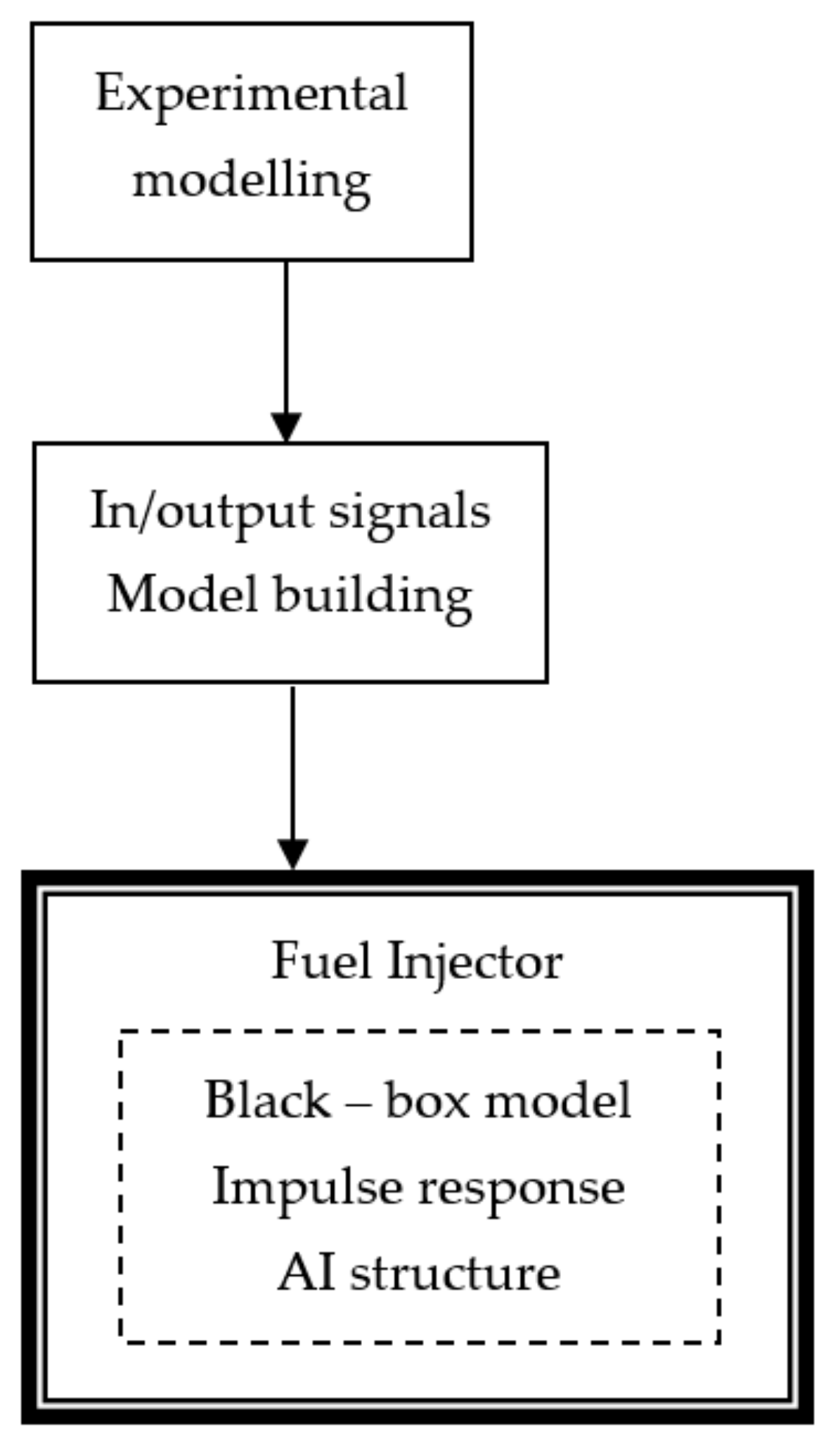
The aim of the research carried out by the Authors is to analyze the possibility of using computational methods on the basis of the model input and output parameters to model the injection doses of a modern Common Rail fuel injector. The fuel injector is the executive element of the engine that is directly responsible for the combustion process in the chamber. Its work consists in providing a given amount of fuel per unit of time with an appropriate structure. The main operating parameters of modern fuel injectors are injection and overflow doses (output parameters). The injection dose is the amount of fuel supplied to the engine’s combustion chamber during one work cycle and expressed as mm3/H, the overflow dose is the discharge of the working liquid during the fuel injector operation and expressed in the same quantities as the injection dose. Each of these quantities must have a specific value for the given engine parameters. The input parameters stimulating the fuel injector to work are the system pressure and the time of its activation. Based on the size of the input parameters, the output parameters are generated. Modern fuel injectors are diagnosed on test benches. The research process of an object consists in assigning it the input parameters (pressure and control time) and reading the output (actual) parameters and comparing them with the set data. The test stands have coordinates (known output quantities) for the selected injector only for its individual input parameters. There are cases where the standard fuel injector test is positive, the engine is not working properly and the symptoms indicate a defect in the injection apparatus. This is because the working areas that are used by the engine are ignored during standard tests. The baseline values are not known when diagnosing the object in these areas. The use of computational methods allows them to be modelled on the basis of known operating characteristics, thanks to which it is possible to determine whether a given injector is operational. The prediction of the operating parameters of a modern injector can be made by the black box method (Figure 1). It is based on the fact that, on the basis of the analysis of the input and output signals of the research object, it is possible to model its work in unknown areas. Polynomial or artificial intelligence algorithms are used to make this type of model. This method is used when the internal dimensions of the object and the exact relations of kinematic connections are not known.
The engine controller, based on the data collected from the sensors, controls the injector operation in such a way as to ensure the appropriate number of doses with a given volume in a given engine work cycle. On the basis of the given input parameters, the operating characteristics of the fuel injector are prepared, which shows the amounts of injection doses at different injector actuation times and system pressures. When the injector malfunctions, its output parameters change, such as the injection or overflow doses, fuel injection delay and the quality of atomization. The general operating characteristics support the diagnostic processes. By using computational methods, the field of research is extended, thanks to which the process of examining the object becomes more accurate. The polynomial and artificial intelligence algorithms proposed by the authors are innovative methods and have not been used in the research processes of the injection apparatus of a modern CI engine yet. The authors of the work [1] described the possibilities of using the Matlab environment to model the operation of technical objects using the black box method. The fuel injector is a device in which it is very difficult to measure the size of the cooperating components. The authors of the work [2] made a mathematical model of a fuel injector. However, this model is designed for a specific injector from a given manufacturer. As ecological requirements increase, leading suppliers of fuel injectors optimize the design, which requires verification of the proposed model, and even developing it from scratch, taking into account various empirically determined parameters in order to reproduce the work of the tested object as closely as possible. This is time-consuming considering the number of available structures.
The job of the fuel injector is to atomize and distribute the right amount of fuel in the combustion chamber of the engine. The work it performs can be considered in terms of quality and quantity. These factors affect the combustion process of the combustible mixture. The amount of the set injection dose is a quantitative aspect and directly affects the combustion of the combustible mixture in the engine compartment.
When analyzing the literature, it can be noticed that most of the research work carried out in terms of the operation of modern fuel injectors is focused mainly on the quality aspect and its diagnostics. Using calculating methods to predict fuel injectors parameters is novelty. The parameter influencing the speed of the fuel at the nozzle outlet is the pressure in the system by Wang et al. [3]. The research conducted by the authors of the study showed that the penetration of the stream in the combustion chamber increases from 1500 MPa to 2100 MPa, however, with increasing pressure in the system, the fuel injection delay increases. Injection delay is the time from the moment the fuel injector is actuated to the moment the fuel is fed to the combustion chamber. This parameter is very important because too long times will result in incorrect engine operation. On average, in the injectors of the CR system, the fuel injection delay is 200–300 μs at the pressure of 80 MPa. In the studies by D’Ambrosio et al. [4] the operating parameters of an electromagnetic and piezoelectric fuel injector were compared. Both injectors were mounted on the same CI engine and its emission of pollutants into the atmosphere and fuel consumption were examined. The differences between the operation of the engine on electromagnetic and piezoelectric fuel injectors are minimal. An important difference between electromagnetic and piezoelectric fuel injectors is their production costs. One of the causes of knocking combustion in the engine is deficiency in the fuel injector. The authors in Taghizadeh—Alisaraei et al. [5] presented a method of diagnosing fuel injectors by reading the vibrations that occur in damaged components. The analysis showed that the damaged elements emit greater vibrations during operation, which affects the size of injection doses. Similar studies were presented by the authors of Hartl et al. [6]. Four fuel injectors were subjected to the analysis. The damaged ones caused a pressure drop in the system due to the higher value of the overflow and additional vibrations. Zhang et al. [7] developed an optical method for diagnosing fuel injectors used in marine CI engines. The method consists in analyzing the quality parameters of the fuel stream. The analysis of the shape of the injected fuel stream may help to assess the technical condition of the atomizer.
Assessment of the condition of individual components can be performed using neural network algorithms. In the study by Uzun [8], an algorithm to calculate the mass of air supplied in a turbocharged engine was developed. The analysis of the test results and calculations has shown that it is possible to apply the above solution in estimating the amount of air supplied to the CI engine. The article by Tosun et al. [9] presented the possibilities of using linear regression and neural network in order to model the operating characteristics of the engine and the emission of toxic substances in exhaust gases. The engine was powered by standard diesel and various types of biofuel. The analysis of the test results showed that the very accurate mapping of the measurements was made with the use of a neural network. In the Matlab environment, using the Neural Network Toolbox add-on, a neural network which tested the operation of the engine was implemented, Liu et al. [10]. Based on parameters such as engine speed, intake air temperature, boost pressure, exhaust gas temperature, engine coolant temperature and fuel consumption, it has been trained for turbocharger diagnostics. The Levenberg-Marquardt algorithm with a square error value of 0.001 was used in the network. The same algorithm was used in the works [11,12,13] to implement neural networks. The research carried out in the work of Stoeck [14,15] describes the possibilities of using statistical methods in a spreadsheet in order to forecast the fuel injector injection doses. When analyzing the results of the conducted experiment, it can be concluded that the use of simple calculation methods and a spreadsheet is inaccurate and limits the number of input variables. The authors of the work [16] used a neural network to estimate the vibration of the engine powered by sunflower oil mixtures. The proposed algorithm was compared with the measurement results and a very high degree of matching was obtained. Also in [17], a model of a neural network was used to determine the vibration for engine diagnostics and compared with the measurement results. The results of the analysis showed a high degree of alignment of the algorithm with the values obtained during the measurements. There is a possibility to implement a neural network to estimate the emission of toxic substances by an engine powered by a vegetable fuel [18,19,20]. The authors achieved agreement of over 95% with the measurement results. Neural Network algorithm has been implemented to predictive vibration in hybrid vehicle powertrain [21]. Simulation showed that proposed model improved conventional method. Authors marked that deep learnings method could be used in many targets. Authors trained neural network estimate emissions for CI engine powered by Biogas [22]. Analysis showed that there has been high matching achieved. The best training algorithm was Levenberg Marquardt. Similar researches has been conducted to predict fuel consumption in the paper [23]. The validation of model reached satisfactory values. Model to predict fuel injection characteristics for various injectors doses could be used in fuel supply system diagnostic and researches. In papers [24,25] Authors proposed the modification of fuel injector nozzle holes. Analysis conducted researches there is possibility to predict for modified injector nozzles injection characteristics using neural networks or polynomial methods. Similar researches has been presented in papers [26,27]. Authors proposed modifications the needle in fuel injector nozzle. Calculating methods could create injection characteristics for modified injectors without testing on the benches.
Analyzing the literature, it can be stated that it is possible to implement computational methods to predict the output parameters of modern fuel injectors. Neural network algorithms have been used in the diagnosis and evaluation of the operation of modern internal combustion engines.
2. Materials and Methods
2.1. Modelling Injection Doses Using a Neural Network
The basic cell of the nervous system is a neuron. It consists of a body called a soma and two types of protrusions surrounding it: introducing dendrite information and deriving axon information. Each neuron has one outlet, thanks to which it sends impulses to other neurons. One neuron transmits information to others through connections called synapses. Synapses act as messengers of information, and as a result of their action, arousal can be strengthened or weakened. As a result, neurons receive information that is stimulating or inhibitory, summing them up. If their algebraic sum exceeds the threshold value, the signal at the output of the neuron is transmitted through the axon to other neurons. The action of neurons can be recorded using the following relationships (1) and (2):
y = f(s),
In the neuron model, n is the number of inputs, x1,…, xn are the input signals, in0,…, wn are synaptic weights, y is the output value and f is the activation function. The work of the neuron is as follows. The input signals are multiplied by the corresponding weights. The values that have been obtained are added up. Then, as a result of the action, an s signal is formed, which maps the linear action of the neuron. In the next stage, this signal is subjected to the activation function. It should be assumed that the signal value of x0 is equal to 1, and the weight in0 is called the threshold. The information is stored in the scales. Learning neurons is based on the right choice of weights.
The process of learning neurons is to calculate the sum of the input product values and the corresponding weights. The obtained value is subjected to the action of an appropriately defined activation function and the output quantity neuron is obtained. Having reference characteristics, it is possible to define an error at the output of the neuron. The errors for the last layer are determined in a similar way in the case of multilayer networks. The problem lies in defining the error value for hidden layers, because without a pattern, the algorithm cannot determine the size of the neurons for these areas. To solve this problem, the error back propagation method should be used. In order to derive this algorithm, the error measure should be defined, which is the function Q(w). In this function, the variables are all weights of the multilayer neural network. Network training consists in finding the minimum of the function Q with respect to the vector w. Then the function should be expanded into the Taylor series in the closest vicinity of the known current solution w, along the p direction, Equation (3) [28].
where g(w) is the gradient vector and H(w) is a matrix of second derivatives.
The operation of the algorithm starts when the training pattern is fed to the network input. First, it is processed by the neurons of the first layer, which determine the output signal. The signals obtained in this way are inputs for the neurons of the next layer. This cycle continues until the last layer. Knowing the output signal of the last layer and the reference signal from the training sequence, it is possible to calculate the error at the network output from the dependence (5). Then, the weights of the last layer neurons are modified using the dependencies (5)–(7). The output error is propagated backwards according to the connections of neurons between the layers and taking into account their dependency activation function (4), (5). The second algorithm on the basis of which the neural network presented in the article was generated is the Levenberg-Marquardt algorithm. It uses the expansion of the Q(w) function expressed by the formula (3) to the third component [28].
The artificial neurons presented in Figure 2, like those in the brain, connect to each other using mathematical models to form multi-layered neural networks.
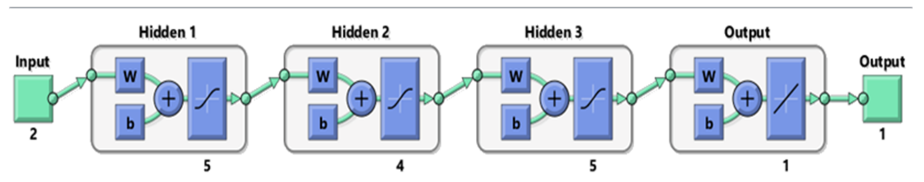
Figure 3 shows a diagram of the neural network created by the authors. It consists of two inputs, pressure in the system and control time, and one output for the injection dose.
2.2. Modelling of Injection Doses with the Use of a Polynomial
The injection dose size modelling was performed in the Matlab environment. Two methods were compared in the work: by means of a polynomial developed with the use of the Curve Fitting Tools application and by the implementation of a neural network.
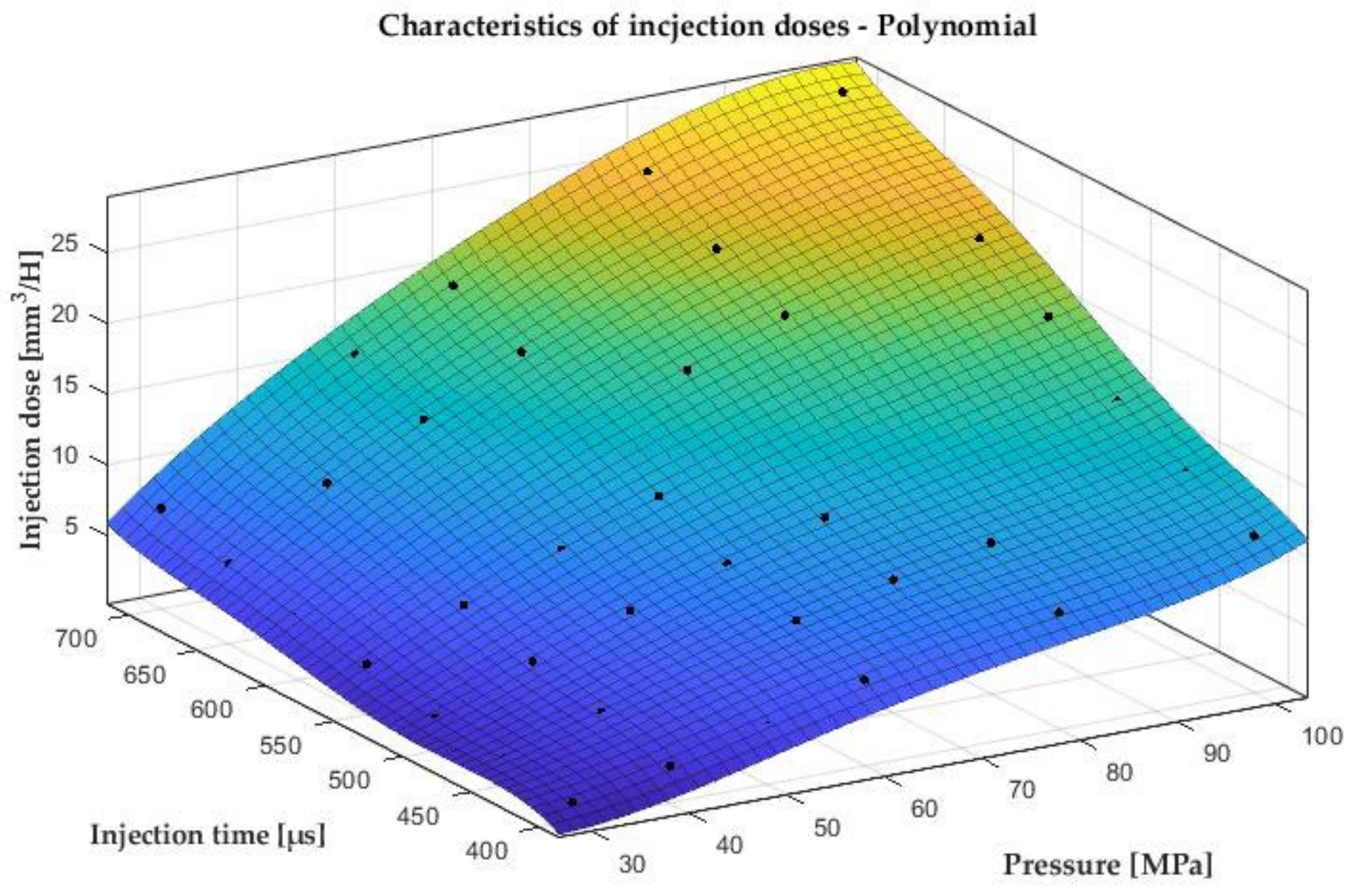
With the help of the Matlab Curve Fitting Tools add-on, a polynomial was developed, on the basis of which a map of possible injection doses was determined depending on two parameters: system pressure and the injector actuation time (Figure 4).
In the case of the conducted analysis, the most favorable results were achieved with a polynomial with a variable x of the fourth degree and y of the fifth degree. On the basis of statistical values such as SSE, R-square, adjusted R-square, RMSE, the accuracy of the developed polynomials to the measurement results was assessed. Thanks to this, we were able to assess which equation most faithfully reproduces the injector’s behavior. Table 1 presents the statistical values.
Statistical values are determined according to mathematical formulas. The sum of squares due error (SSE) is determined from the following Equation (8).
where Yi is the actual value of the dependent variable, Ŷi—predicted value of the dependent variable based on the regression model.
The SSE is the sum of the deviations of the Yi value from the regression line. This coefficient equal to zero occurs with a perfect fit of the model. When evaluating different variants of a polynomial, care should be taken to keep the SSE as close to zero as possible.
The R-square factor is a measure of the quality of a model fit. It is also called the coefficient of determination. This coefficient takes values from 0 to 1. However, the closer to the value 1, the more accurate the model. The coefficient of determination is calculated from the following relationship (9).
where is the predicted value of the dependent variable based on the regression model, Yi is the actual value of the dependent variable, is the mean value of the actual dependent variable.
The task of the adjusted R-square determination coefficient is to eliminate useless explanatory variables from the model.
Adjusted R-square—is the modified R-square factor. The above factor is determined from the following formula (10):
where: b—the number of observations, m—the number of explanatory variables.
The above coefficient is very useful when we have several polynomials with an approximate R-squared value and at this point it is difficult to clearly state which proposed model is better. The use of the adjusted coefficient of determination solves this problem and indicates more precisely which polynomial proposed in this case is more accurate. It is worth noting that the above factor will always be less than the R-squared factor.
The RMSE (root mean squared error) is a measure of the difference between the values predicted by the model and the observed values. The closer the value is to zero, the more accurate the model. The formula is as follows, relations (11) and (12):
where: SSE is Sum of squares due error, v is the number of samples.
3. Results
The method of predicting injection doses can be used in the diagnosis of modern fuel injectors. The tested Volvo C30 vehicle with a 1.6D engine worked unevenly at the engine speed of 1500–1700 rpm. The vehicle uses piezoelectric fuel injectors from VDO Continental Siemens of the 2nd generation. Standard testing on the Zapp Carbon Tech CRU2i test bench showed that all of them were operational (Table 1). Only additional tests with the STPiW 3 test bench showed that one injector works incorrectly in a small dosing area.
By analyzing the Table 2, it can be concluded that all doses of the tested fuel injector are normal. In order to diagnose improper engine operation, a number of additional operating characteristics were made. One of them showed an anomaly in the range of control times of 525–625 µs at a system pressure of 40–60 MPa (Figure 5). Finding this area was time-consuming and expensive.
It is possible to accelerate the processes of diagnostics of injection equipment components by using computational methods. The authors of the work developed two computational methods in the Matlab environment that estimate the output parameters of the fuel injectors on the basis of the input values using the developed polynomial and the “learned” neural network. The neural network algorithm created in the Matlab Deep Learning Toolbox application was learned thanks to the measurements obtained from the STPiW3 test bench. The test bench automatically performed the operating characteristics. On the basis of the measurement results, the areas of improper operation of the fuel injector have been identified.
Laboratory tests were carried out on a test bench for testing the components of the high-pressure CR system of the STPiW3 type. The test stand enables measurements of the operating parameters of the fuel injector, such as: the size of injection and overflow doses as well as tightness. The research object was a piezoelectric Common Rail fuel injector manufactured by VDO Continental Siemens of the 2nd generation, catalogue number 9674973080. The analysis was performed according to the following program: preparation of the standard characteristics of the fuel injector, preparation of the characteristics of the tested fuel injector proposed by the authors, preparation of the characteristics model using a polynomial and a neural network proposed by the authors. The base characteristic was the standard characteristic of the tested injector.
The first stage of the research was to perform its standard operating characteristics on the STPiW 3 test bench shown in Figure 6.
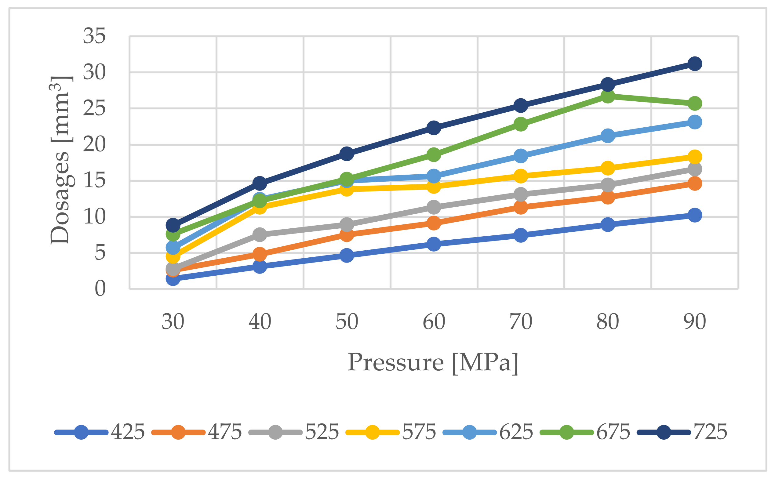
The standard characteristic is based on the following measuring points: pressures 30, 40, 50, 60, 70, 80 and 100 MPa for fuel injector actuation times of 400, 450, 500, 550, 600, 650 and 700 μs. Then, another reference characteristic with changed parameters was performed on the test bench: system pressures 30, 40, 50, 60, 70, 80 and 90 MPa, fuel injector actuation times 425, 475, 525, 575, 625, 675 and 725 μs, Figure 7.
Then, based on the standard operating characteristics (Figure 6) of the tested injector, using polynomials in the Matlab environment, the injection doses were modelled, Figure 8.
Figure 9 shows the deviations of the measurements and predictions of the injection doses for individual control times of the tested fuel injector using a polynomial. The measuring error of the test bench is 2% according to the manufacturer’s data. The table was calibrated before taking the measurements.
Figure 10 shows percentage deviations between measurements and predictions of the injection doses using the polynomial.
Based on the standard operating characteristics (Figure 6) of the tested injector, using polynomials in the Matlab environment, the injection doses were modelled, Figure 11.
A similar analysis was performed for the implementation of the neural network. On the basis of the measurements presented in Figure 6, the injection doses were modelled using the implementation of a neural network. The results were compared with the measurements made during the test in Figure 7 and presented in Figure 12.
Figure 13 shows percentage deviations between measurements and predictions of the injection doses using the neural network.
Injection dose prediction analysis was carried out in the Matlab Deep Learning Toolbox environment using reverse error propagation algorithms and its Levenberg-Marquardt modification. A network consisting of three hidden layers was designed for analysis. The advantage of such a solution is the ability to define any area. Based on the analysis of the literature [20], the optimal combination of networks should be structure 5—5—5. During the research, it turned out that the proposed combination is not optimal due to an error during the calculation, which ranged from 0.7564 to 2.5320 and the difference is 1.7756. It was necessary to make a modification, which consisted in finding such a structure from three layers so that the error was as small as possible. A dependency was used for the analysis (13):
where:
- sbb—average absolute error
- Xi—fuel injection dosage measured on the test bench
- Yi—fuel injection dosage calculated by neural network
- n—the number of researched dosages
On the basis of the calculations carried out, a structure in the form of 5—4—5 was created. The smallest error of this structure was 0.7605 and the largest was 0.9960, which gives a difference r 0.2355.
After selecting the appropriate structure of the neural network, we started to train it in order to achieve the lowest possible error. From our attempts at learning our structure, the lowest absolute error of the neural network was achieved at the level of 0.6682.
When analyzing the above characteristics and the results presented in Figure 14 and it can be noticed that the largest dose error occurs near the greatest workload of the injector and the maximum difference is at the level of 4.3016, i.e., approx. 16.28%. When checking other network structures, the biggest errors were also found around the highest load.
When analyzing Figure 15 and Figure 16, it can be seen that the characteristics are comparable at the lowest loads. The differences are most noticeable at the highest loads. The solution to this problem may be to make a wider injector characteristics on the test bench in order to provide a larger database for learning. It is worth mentioning a very important point. For research purposes, in the application of the neural network for testing injectors, two characteristics of the same injector have been used.
The operating characteristics of the tested fuel injector (Figure 7) served as the basis for learning the neural network. The additional characteristics proposed by the authors (Figure 6) were performed under different operating conditions and served as the test against which the neural network error was calculated. Such a procedure was aimed at proving that the network was not overtrained, which manifests itself in a large dose error in conditions in which the neural network was not trained.
4. Discussion
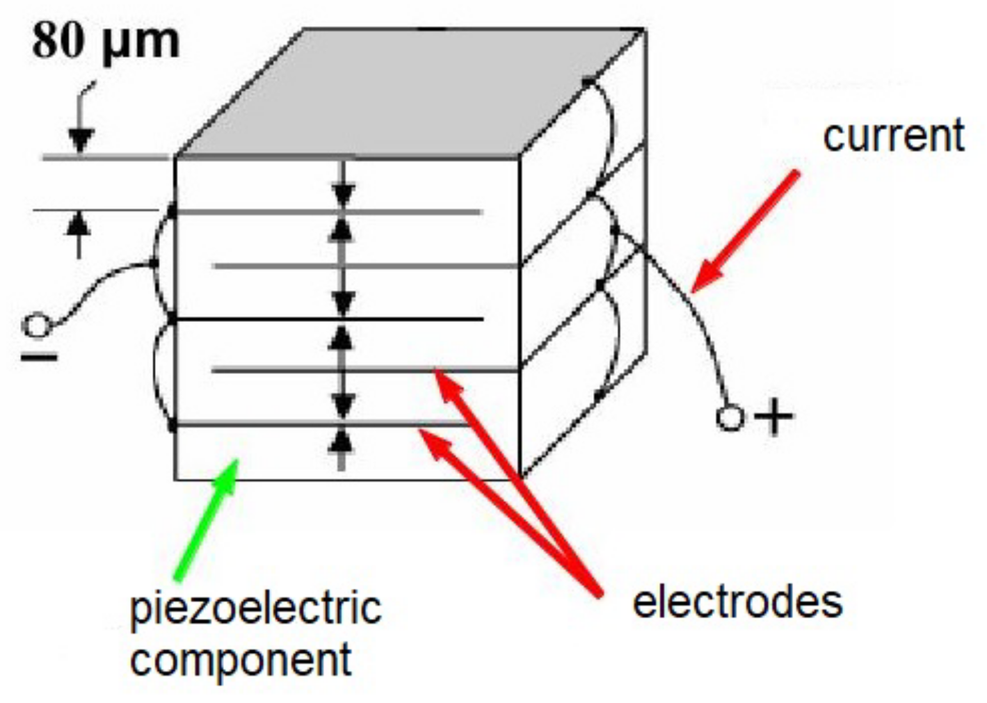
The presented method of injection dose prediction can be used to support the diagnostic processes of modern fuel injectors, especially piezoelectric ones. The element controlling the valve operation of such a fuel injector is a pile of crystals.
The stack of crystals (Figure 17) consists of 350 piezoelectric elements. After applying the voltage, each of them extends by 13 μm, in total the entire element changes its length by 4550 μm. The test of the stack consists in measuring its resistance at a voltage of 150 V. If the resistance is 180–200 kΩ, the stack is functional. Unfortunately, sometimes despite the tests carried out, where the result was normal and the fuel injector did not work properly due to the ailments of individual crystals.
The research showed that the values of the deviation of individual crystals change during operation. This leads to an anomaly during the operation of the fuel injectors within a certain range. Detecting this type of fault is laborious, therefore the use of the numerical method may speed up the process.
In the article, the authors used two methods to determine the characteristics of the injector on the basis of measurement data from the test bench. The first one is polynomial interpolation, where a polynomial has been determined using an appropriate algorithm, which determines the performance characteristics of the tested object. Analyzing the results of calculations, the mean error is 0.56976 mm3/H, the maximum error is 4.34 mm3/H and the minimum one is 0.77 mm3/H (Table 3).
The second method is a neural network with three hidden layers of the structure 5—4—5, where the strength of this method are the weight values determined by the Levenberg—Marquardt algorithm. Analyzing the results, the average error is 0.48 mm3/H, the maximum error is 4.30 mm3/H and the minimum error is 0.64 mm3/H (Table 4).
By analyzing the results of the calculations, it can be concluded that the average injection dose errors determined by the polynomial and the neural network are approximate. A minimally smaller deviation occurs when the neural network is used. It is worth noting that both in the neural network and in the polynomial, the greatest errors appear at the highest loads of the injector. The solution may be to extend the characteristics of the injector in order to provide a larger database necessary for learning the neural network and determining the polynomial. The use of the polynomial approximation method is a better solution having only two input parameters and one output parameter. The prediction does not depend on the randomness of the initial data, such as weights in the neural network. Every time an attempt is made to generate a polynomial, the same result is always obtained. However, in the case of diagnostics, where there are more than two input parameters, a much better method is to use a neural network. Nevertheless, this method requires more analysis in terms of the selection of the number of hidden layers, the number of neurons and the selection of the method of backward error propagation. It is often necessary to analyze multiple combinations of structures in order to assess which combination is the most optimal and most likely to be successful for diagnostic purposes and to correctly predict the performance of the injector under given conditions. In addition, a serious disadvantage of this method is the large influence of randomly selected weights at the initial stage of learning the neural network. The application of computational methods, in particular neural networks, is an innovative method that has not been used yet in the field of diagnostics and prediction of fuel injectors operation.
5. Conclusions
In this study Authors proposed use mathematical methods to calculate modern fuel injector work parameters. The methods has been based on black box modelling. Presented type of calculating is very helpful for objects with complicated construction. Fuel injector consists with kinematics elements. The correlations between them are made with very high precision. So that standard modelling is very hard to calculating and for every injector should be done separately. Authors method is universal for all injectors, because artificial intelligence and polynomial basing on in and output signals.
The conducted analysis showed that it is possible to use computational methods to predict the size of the output parameters of modern injection equipment. The research showed that both the polynomial and the artificial intelligence method mapped the injection doses with a very good fit for low and medium load. The average error for neural network method was 5.34% and for polynomial 6.63%. The analysis of Table 3 and Table 4 shows that minimum error for polynomial is 0.77 mm3/H and maximum 4.34 mm3/H and for artificial network minimum 0,64 mm3/H and maximum 4.30 mm3/H. The differences are not high but, neural network is better because gives the possibilities to use more variables. Polynomial method is good solution for only two variables, not more.
The implementation of a polynomial or an artificial intelligence algorithm to the test bench controller supports the processes of diagnosing modern fuel injectors, especially piezoelectric ones. The authors are currently working on improving the proposed methods in terms of the maximum workload of the injectors in order to increase the range of the predictive model for each injector input parameter that affects the fuel dose.
Author Contributions
The scope of work of individual authors during the performance of this project was the same. The authors performed the study together and then analyzed its findings. The paper was written together. The writers of the paper were T.O., K.F.A. and Ł.M. All authors have read and agreed to the published version of the manuscript.
Funding
This research received no external funding.
Institutional Review Board Statement
Not applicable.
Informed Consent Statement
Not applicable.
Data Availability Statement
Not applicable.
Conflicts of Interest
We do not have any personal conflicts of interest in communicating the findings of this study, and we had no sponsor who would make claims to the findings being presented.
References
- Garnier, H.; Gilson, M. Contsid: A matlab toolbox for standard and advanced identification of black-box continuous-time models. IFAC Pap. Online 2018, 51, 688–693. [Google Scholar] [CrossRef]
- Marcic, S.; Marcic, M. Mathematical Model for the Injector of a Common Rail Fuel-Injection System. Engineering 2015, 7, 307. [Google Scholar] [CrossRef] [Green Version]
- Wang, L.; Lowrie, J.; Ngaile, G.; Fang, T. High injection pressure diesel sprays from a piezoelectric fuel injector. Appl. Therm. Eng. 2019, 152, 807–824. [Google Scholar] [CrossRef]
- D’Ambrosio, S.; Ferrari, A. Diesel engines equipped with piezoelectric and solenoid injectors: Hydraulic performance of the injectors and comparison of the emissions, noise and fuel consumption. Appl. Energy 2018, 211, 1324–1342. [Google Scholar]
- Taghizadeh-Alisaraei, A.; Mahdavian, A. Fault detection of injectors in diesel engines using vibration time-frequency analysis. Appl. Acoustic. 2019, 143, 48–58. [Google Scholar] [CrossRef]
- Hartl, F.; Brueckner, J.; Ament Ch Provost, J. Rail Pressure Estimation for Fault Diagnosis in High Pressure Fuel Supply and Injection System. IFAC–Pap. Online 2019, 52, 193–198. [Google Scholar] [CrossRef]
- Zhang, W.; Li, X.; Huang, L.; Feng, M. Experimental study on spray and evaporation characteristics on diesel-fueled marine engine based on optical diagnostic technology. Fuel 2019, 246, 454–465. [Google Scholar] [CrossRef]
- Uzun, A. Air mass flow estimation of diesel engines using neural network. Fuel 2014, 177, 833–838. [Google Scholar] [CrossRef]
- Tosun, E.; Aydin, K.; Bilgili, M. Comparison of linear regression and artificial neural network model of a diesel engine fueled with biodiesel-alcohol mixtures. Alex. Eng. J. 2016, 55, 3081–3089. [Google Scholar] [CrossRef] [Green Version]
- Liu, B.; Zhao, C.; Zhang, F.; Cui, T.; Su, J. Misfire detection of a turbocharged diesel engine by using artificial neural networks. Appl. Therm. Eng. 2013, 55, 26–32. [Google Scholar] [CrossRef]
- Iscan, B. ANN modeling for justification of thermodynamic analysis of experimental applications on combustion parameters of a diesel engine using diesel and safflower biodiesel fuels. Fuel 2020, 279, 118391. [Google Scholar] [CrossRef]
- Celebi, K.; Uludamar, E.; Tosun, E.; Yildizhan, S.; Aydin, K.; Ozcanli, M. Experimental and artificial neural network approach of noise and vibration characteristics of an unmodified diesel engine fuelled with conventional diesel, and biodiesel blends with natural gas addition. Fuel 2017, 197, 159–173. [Google Scholar] [CrossRef]
- Ismail, H.M.; Ng, H.K.; Queck, C.W.; Gan, S. Artificial neural networks modelling of engine-out responses for a light-duty diesel engine fuelled with biodiesel blends. Appl. Therm. Energy 2012, 92, 769–777. [Google Scholar] [CrossRef]
- Stoeck, T. Simplification of the procedure for testing common rail fuel injectors. Combust. Engines 2020, 180, 52–56. [Google Scholar] [CrossRef]
- Stoeck, T. Methodology for Common Rail fuel injectors testing in case of non-typical faults. Diagnostyka 2020, 21, 25–30. [Google Scholar] [CrossRef]
- Böyükdipi, Ö.; Tüccar, G.; Soyhan, H.S. Experimental investigation and artificial neural network (ANNs) based prediction of engine vibration of a diesel engine fueled with sunflower biodiesel-NH3 mixtures. Fuel 2021, 304, 121462. [Google Scholar] [CrossRef]
- Qin, C.; Jin, Y.; Tao, J.; Xiao, D.; Yu, H.; Liu, C.; Shi, G.; Lei, J.; Liu, C. DTCNNMI: A deep twin convolutional neural networks with multi-domain inputs for strongly noisy diesel engine misfire detection. Measurement 2021, 180, 109548. [Google Scholar] [CrossRef]
- Hoang, A.T.; Nizetic, S.; Ong, H.C.; Tarelko, W.; Pham, V.V.; Le, T.H.; Chau, M.Q.; Nguyen, X.P. A review on application of artificial neural network (ANN) for performance and emission characteristics of diesel engine fueled with biodiesel-based fuels. Sustain. Energy Technol. Assess. 2021, 47, 101416. [Google Scholar]
- Subramanian, K.; Sathiyagnanam, A.P.; Damodharan, D.; Sivashanmugam, N. Artificial Neural Network based prediction of a direct injected diesel performance and emission characteristics powered with biodiesel. Mater. Today Proc. 2021, 43, 1049–1056. [Google Scholar] [CrossRef]
- Castresana, J.; Gabina, G.; Martin, L.; Uriondo, Z. Comparative performance and emissions assessments of a single cylinder diesel engine using artificial neural network and thermodynamic simulation. Appl. Therm. Eng. 2021, 185, 116343. [Google Scholar] [CrossRef]
- Ogawa, H.; Takahashi, Y. Echo State Network Based Model Predictive Control for Active Vibration Control of Hybrid Electric Vehicle Powertrains. Appl. Sci. 2021, 11, 6621. [Google Scholar] [CrossRef]
- Mandal, A.; Cho, H.; Chauhan, B.S. ANN Prediction of Performance and Emissions of CI Engine Using Biogas Flow Variation. Energies 2021, 14, 2910. [Google Scholar] [CrossRef]
- Ziółkowski, J.; Oszczypała, M.; Małachowski, J.; Szkutnik-Rogoż, J. Use of Artificial Neural Networks to Predict Fuel Consumption on the Basis of Technical parameters of Vehicles. Energies 2021, 14, 2639. [Google Scholar] [CrossRef]
- Beatrice, C.; Belgiorno, G.; Di Blasio, G.; Mancaruso, E.; Sequino, L.; Vagliego, B.M. Analysis of a Prototype High-Pressure “Hollow Cone Spray” Diesel Injector Performance in Optical and Metal Research Engines. SEA Tech. Pap. 2017, 24, 73. [Google Scholar]
- Sequino, L.; Belgiorno, G.; Di Blasio, G.; Mancaruso, E.; Beatrice, C.; Vagliego, B.M. Assessment of the New Features of a Prototype High-Pressure “Hollow Cone Spray” Diesel Injector by Means of Engine Performance Characterization and Spray Visualization. SEA Tech. Pap. 2018, 1, 1697. [Google Scholar]
- Eliasz, J.; Osipowicz, T.; Abramek, K.F.; Mozga, Ł. Model Issues Regarding Modification of Fuel Injector Components to Improve the Injection Parameters of a Modern Compression Ignition Engine Powered by Biofuel. Appl. Sci. 2019, 9, 5479. [Google Scholar] [CrossRef] [Green Version]
- Eliasz, J.; Osipowicz, T.; Abramek, K.F.; Matuszak, Z.; Mozga, Ł. Fuel Pretreatment Systems in Modern CI engines. Catalysts 2020, 10, 696. [Google Scholar] [CrossRef]
- Rutkowski, L. Metody I Techniki Sztucznej Inteligencji; Wydawnictwo Naukowe PWN: Warszaw, Poland, 2012. [Google Scholar]
Figure 1.
Black box calculating model.

Figure 2.
Structure of the neuron.

Figure 3.
A diagram of a neural network that allowed to create a brain that determines the dose of injectors depending on pressure and time.
Figure 3.
A diagram of a neural network that allowed to create a brain that determines the dose of injectors depending on pressure and time.

Figure 4.
Characteristics of injection doses depending on pressure and injection time. X axis—pressure [MPa], Y axis—injection time [µs], Z axis—injection dose [mm3/H].
Figure 4.
Characteristics of injection doses depending on pressure and injection time. X axis—pressure [MPa], Y axis—injection time [µs], Z axis—injection dose [mm3/H].

Figure 5.
Fuel dosages graph of a damaged injector (anomaly in the range of control times 525–625 μs at a system pressure 40–60 MPa) with an incorrect dosing area.
Figure 5.
Fuel dosages graph of a damaged injector (anomaly in the range of control times 525–625 μs at a system pressure 40–60 MPa) with an incorrect dosing area.

Figure 6.
Fuel dosages graph of the tested injector.

Figure 7.
Fuel dosages graph of the tested injector proposed by the authors—parameters measured on the STPiW 3 test bench.
Figure 7.
Fuel dosages graph of the tested injector proposed by the authors—parameters measured on the STPiW 3 test bench.

Figure 8.
Fuel dosages graph of the tested injector modelled with the use of a polynomial, proposed by the Authors.
Figure 8.
Fuel dosages graph of the tested injector modelled with the use of a polynomial, proposed by the Authors.

Figure 9.
Comparison of differences between measured and calculated by polynomial operational parameters of the tested injector.
Figure 9.
Comparison of differences between measured and calculated by polynomial operational parameters of the tested injector.

Figure 10.
Comparison of differences between the operating parameters measured and presented by the polynomial of the tested injector.
Figure 10.
Comparison of differences between the operating parameters measured and presented by the polynomial of the tested injector.

Figure 11.
Fuel dosages graph of the tested injector modelled with the use of a neural network, proposed by the Authors.
Figure 11.
Fuel dosages graph of the tested injector modelled with the use of a neural network, proposed by the Authors.

Figure 12.
Comparison of differences between the operating parameters measured and presented by the neural network of the tested injector.
Figure 12.
Comparison of differences between the operating parameters measured and presented by the neural network of the tested injector.

Figure 13.
Comparison of differences between the operating parameters measured and presented by the neural network of the tested injector.
Figure 13.
Comparison of differences between the operating parameters measured and presented by the neural network of the tested injector.

Figure 14.
Characteristics of the mean error between the output data from the test bench and the obtained from the neural network.
Figure 14.
Characteristics of the mean error between the output data from the test bench and the obtained from the neural network.

Figure 15.
Injection dose size characteristics obtained from measurements on the test bench.

Figure 16.
Injection dose size characteristics obtained as a result of the implementation of a neural network.
Figure 16.
Injection dose size characteristics obtained as a result of the implementation of a neural network.

Figure 17.
Piezoelectric crystals stack.


Table 1.
Statistical polynomial fit values.
| Statistical Values | Pressure Volumes |
|---|---|
| SSE | 3.217 |
| R-square | 0.9985 |
| Adjusted R-square | 0.9975 |
| RMSE | 0.3331 |
Table 2.
Fuel injector standard test results.
| Dose Type | Test Parameters | Correct Dose Range [mm3/H] | Measurement Results [mm3/H] |
|---|---|---|---|
| VTP I | 160 MPa 1000 µs | 37.52–51.92 | 47.83 |
| VTP II | 46 MPa 500 µs | 9.43–14.23 | 11.34 |
| VTP III | 72 MPa 660 µs | 15.66–29.10 | 22.18 |
| VTP IV | 22 MPa 370 µs | 0.50–4.76 | 3.65 |
Table 3.
The error between the dose value calculated by the polynomial and the dose value obtained from the measurements on the test bench.
Table 3.
The error between the dose value calculated by the polynomial and the dose value obtained from the measurements on the test bench.
| 30 | 40 | 50 | 60 | 70 | 80 | 90 | |
|---|---|---|---|---|---|---|---|
| 425 | −0.77 | −0.24 | −0.55 | −0.53 | −0.62 | −0.25 | −0.17 |
| 475 | 0.15 | 0.28 | 0.61 | 0.37 | 0.85 | 0.99 | 1.38 |
| 525 | 0.04 | 0.47 | 0.41 | 0.05 | 0.3 | −0.09 | 0.45 |
| 575 | −0.09 | 0.1 | −0.33 | −0.52 | −0.39 | −0.6 | −0.29 |
| 625 | −0.05 | −0.16 | 0.07 | 0.28 | 1.11 | 1.64 | 1.3 |
| 675 | 0.81 | 1.5 | 1.28 | 1.59 | 2.24 | 3.54 | 0.46 |
| 725 | 0.6 | 0.89 | 0.81 | 1.63 | 4.34 | 1.01 | 2.02 |
Table 4.
The error between the dose calculated at the neural network and the dose obtained from the measurements on the test bench.
Table 4.
The error between the dose calculated at the neural network and the dose obtained from the measurements on the test bench.
| 30 | 40 | 50 | 60 | 70 | 80 | 90 | |
|---|---|---|---|---|---|---|---|
| 425 | −0.32 | 0.01 | −0.30 | 0.09 | −0.08 | −0.56 | −0.61 |
| 475 | 0.32 | −0.31 | 0.65 | 0.59 | 0.60 | 0.64 | 0.99 |
| 525 | −0.02 | −0.26 | 0.20 | −0.13 | 0.44 | 0.07 | 0.47 |
| 575 | −0.21 | −0.05 | −0.33 | −0.06 | 0.09 | −0.49 | −0.64 |
| 625 | −0.03 | −0.10 | 0.12 | 0.45 | 1.06 | 1.37 | 1.12 |
| 675 | 0.97 | 1.47 | 0.88 | 1.26 | 2.42 | 4.30 | 1.49 |
| 725 | −0.15 | 0.53 | 0.67 | 1.63 | 1.24 | 0.68 | 1.27 |
Publisher’s Note: MDPI stays neutral with regard to jurisdictional claims in published maps and institutional affiliations. |
© 2022 by the authors. Licensee MDPI, Basel, Switzerland. This article is an open access article distributed under the terms and conditions of the Creative Commons Attribution (CC BY) license (https://creativecommons.org/licenses/by/4.0/).
Share and Cite
MDPI and ACS Style
Osipowicz, T.; Abramek, K.F.; Mozga, Ł. Comparing Polynomials and Neural Network to Modelling Injection Dosages in Modern CI Engines. Appl. Sci. 2022, 12, 2246. https://doi.org/10.3390/app12042246
AMA Style
Osipowicz T, Abramek KF, Mozga Ł. Comparing Polynomials and Neural Network to Modelling Injection Dosages in Modern CI Engines. Applied Sciences. 2022; 12(4):2246. https://doi.org/10.3390/app12042246
Chicago/Turabian StyleOsipowicz, Tomasz, Karol Franciszek Abramek, and Łukasz Mozga. 2022. "Comparing Polynomials and Neural Network to Modelling Injection Dosages in Modern CI Engines" Applied Sciences 12, no. 4: 2246. https://doi.org/10.3390/app12042246
Note that from the first issue of 2016, this journal uses article numbers instead of page numbers. See further details here.