ANN Prediction of Performance and Emissions of CI Engine Using Biogas Flow Variation

Abstract

Compression ignition (CI) engines are popular in the transport sector because of their high compression ratio. However, in recent years, it has become a major concern from an environmental point of view because of the emission and depleting fossil fuel. The advanced combustion concept has been a popular research topic in the CI engine. Low-temperature combustion with alternate fuel has helped in reducing the oxides of nitrogen (NO_x) and soot emission of the engine. Biogas is a popular substitute of energy especially deduced from biomass because of its clean combustion properties, as well it being a renewable energy source compared to non-renewable diesel resources. In experiments with dual fuel, i.e., conventional diesel and alternate fuel (biogas) were carried out through them. In the present study, an artificial neural network model was used to estimate emissions and check the attributes of performance. Different algorithms and training functions were used to train the models. However, the best training algorithm was Levenberge Marquardt and the training function was Tansig (Hyperbolic tangent sigmoid) and Logsig (logarithmic sigmoid), which showed the best result with regression coefficient (R > 0.98) and Mean square error (MSE < 0.001). The best model was trained by evaluating MSE and regression coefficient. Experimental results and artificial neural network (ANN) prediction showed that the experimental results were similar to each other and lie at the same intervals. The ANN model helped in predicting experimental data that were earlier difficult to experimentally perform using interpolation and extrapolations. It was observed that there was an increase in Brake Specific Energy Consumption (BSEC) and a decrease in Brake thermal efficiency (BTE) with improved biogas flow rate and reduced NO_x emission in the combustion chamber. Carbon monoxide (CO) and hydrocarbon (HC) emissions increase linearly with the increase in biogas flow rate, whereas smoke opacity decreases. It could be concluded that this study helps in understanding the effect of dual fuel (diesel-biogas) combustion under different load conditions of the engine with the help of ANN, which could be a substitute fuel and help to protect the environment.

1. Introduction

In recent years, the interest in alternate fuels and renewable energy [1] has increased because of an increase in energy demand [2] and stringent environmental policies [3], which are because of the depleting fossil fuels, and an increase in the price of fossil fuels for the internal combustion engine [4]. A compression ignition engine is being used by the transportation sector and holds a major share [5]. It was also observed that conventional compression ignition (CI) engines had higher NO_x and soot. To control the emissions, exhaust gas recirculation and an after-treatment method (diesel particulate filter, diesel oxidation catalyst, and selective catalytic reduction), or both, were incorporated together. Incorporating these systems in the engine increases the complexity and cost of the engine. Advance combustion concepts and specific fuels were the topics of interest for many researchers [6]. Energy demand has been increasing [7] and demand for decarbonization is important for the environment [8]. Therefore, an urgent need for alternate fuels is required for the CI engine [9], both liquid as well as gases [10,11]. In the case of IC engines, gaseous alternate fuel can be considered because of their high compression ratio [12] and good mixing characteristics, which in turn would decrease the emission and increase brake thermal efficiency [13].

For the CI engine, advanced combustion strategies such as:

• Reactivity controlled compression ignition (RCCI)
• Homogeneous charge compression ignition (HCCI)
• Partially premixed combustion (PPC) were used

NO_x and soot emissions were reduced by partial premix combustion when applied to the IC engine. PPC helped in reducing heat transfer losses and shortened the combustion duration compared to conventional diesel engines. Other researchers mixed low-temperature combustion with alternate fuels (ethanol, butanol, natural gas, butanol, bio-methane, etc.) [14,15]. Bio-methane has been a popular alternate fuel in Poland and Italy. It could be developed from animal slurry, biodegradable waste, and from maize grown on agricultural land [16,17]. This combination showed improvement in NO_x, soot emissions and efficiency. Generally, in dual-fuel combustion, one of the fuels is of high reactivity and the other is of low reactivity [18]. Biomethanol, as an alternative fuel in the transport and industrial sector, needs to be investigated [19].

A potential renewable energy is biogas, which could be produced from organic material under natural degradation by micro-organisms without the use of oxygen. Organic substances are converted to biogas by anaerobic digestion, which is used as fuel for vehicles and to generate heat and electricity. Biogas mainly constitutes of methane and carbon dioxide [20]. Biogas for industrial purposes is developed at (1) landfills, (2) agricultural organic waste digestion plants, (3) sewage treatment plants, and (4) sites with industrial processing units [21].

Biogas is environment friendly [22] and is available abundantly [23,24]. The use of biogas in the CI engine is difficult, as there is no spark plug for combustion and ignition. Biogas is also low in cetane number and has a high self-ignition temperature [25]. CO₂ composition of biogas helps in combustion at low temperature, which reduces the chance of NO_x emission formation at elevated temperature during combustion in dual fuel mode [26,27]. BTE remains unchanged for intermittent loads, whereas, at reduced loads, it decreases and increases at maximum loads [28,29]. Thus, by using biogas as a dual fuel mode [30], smoke and NOx emission were reduced and controlled [31,32].

Karthic et al. used an artificial neural network to foreshow the performance and emission of a diesel engine. The ANN model has input parameters such as the load on the engine, the injection pressure of fuel, fuel flow rate and injection timing of fuel; and the output parameters of the model were brake thermal efficiency and emission. It was evident that the experimental results and the ANN prediction were similar for the dual-fuel engine in terms of emission and performance [33]. Gul et al. obtained the optimum combination of engine speed, operating load and fuel nature by Taguchi DOE in a diesel engine that was run by 100% waste cooking oil and B20 (i.e., 20% biodiesel and 80% diesel). Experimental results and ANN simulation computed the best combination by guaranteeing refinement of the output response factors, thus ratifying the Gray–Taguchi method in curtailing emissions and enhancing combustion and performance simultaneously [34]. To conduct the experiment, Kumar used RSM based on box-Behnken experimental design. For the production of jatropha-algae oil, parameters such as the molar ratio, reaction time, catalyst concentration, and reaction temperature were optimized. The predicted results showed a correlation with the RSM outcomes [35]. Samuel et al. modeled the production of coconut oil ethyl ester by RSM and ANN. It was observed that the predicted yield by ANN agreed with the output of the experiment [36]. Calik et al. (2018) used corn, sunflower and canola biodiesel blends in a diesel engine, injected hydrogen through a manifold inlet and predicted the emission, noise and vibration level with the help of a support vector machine and artificial neural network. It was concluded that ANN predicted better results than SVM [37]. Najafi et al. (2019) experimented on a CI engine, which was simultaneously run by pilot fuel (oxygenated additive) and main fuel (natural gas). Artificial Neural Network and genetic algorithm modeling were used to reduce emission by establishing the ratio of pilot fuel in respect to biodiesel, gaseous fuel, and additive [38]. Javed et al. used hydrogen fuel with ZnO nano additives biodiesel in a diesel engine. An artificial neural network was utilized to forebode noise with different engine criteria. ANN was also used so that extensive experimentation could be avoided.

This paper examined the performance and emission features under the influence of diesel and biogas used together at varying engine loads at different gas flow rates. The prediction of performance and emission was carried out by an artificial neural network [39]. Biogas was introduced into the combustion chamber through an inlet manifold. The comparative analysis of the prediction and the actual data are presented in this paper.

2. Experimental Setup

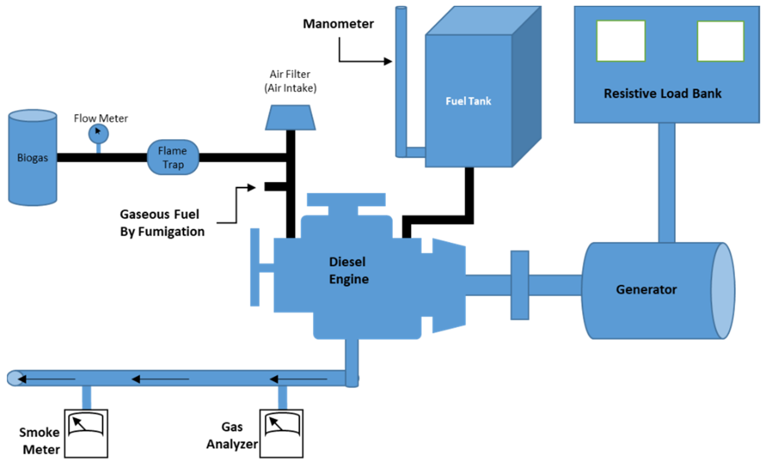
DAF8 Kirloskar make, single cylinder engine, four stroke-naturally aspirated, with a power of 6 kW was employed in the experiment. The experimental setup is shown in Figure 1. In India, such single-cylinder CI engines are mostly used in agriculture and for commercially generating electricity applications in rural areas.

Table 1. Engine specification for experimentation.

Company	Kirloskar Oil India Ltd.
Model	DAF8
Bore × stroke	95 × 110 mm
Power	8 BHP
Speed (RPM)	1500
Inlet valve opening (degree)	4.5°
Inlet valve closed (degree)	35.5°
Exhaust valve opening (degree)	35.5°
Exhaust valve closed (degree)	4.5°
Injection type	Direct Injection
Nozzle opening pressure	200 bar
No. of holes (diesel injector)	4
Cylinder’s	1
Compression ratio	17.5:1
Cylinder volume	780 cc
Static injection timing	26° bTDC
Alternator Specifications
Company	Kirloskar Private Limited
Dynamometer	AC alternator,50 Hz, single phase
Current rating	21.7 A
Rated output	5 kVA
Voltage rating	230 V
Rated speed	1500 rpm
Boundary Conditions
Intake temperature	Room temperature
Boost pressure	205–210 bar
Injection quantity	0–10 kg/h
Injection strategy	Single Point

depicts the specification of the CI engine employed for the experiment. Properties of different fuels used for the experiment are enlisted in

Table 2. Fuel attributes.

Attributes	Biogas	Diesel
Chemical Composition	CH4 (60%), CO2 (40%) (volume)	C12H26
Cetane Number	-	45–55
Density (kg/m3)	1.1	840
Auto-ignition temperature (K)	1086	553
Lower Calorific Value (MJ/kg)	20.67	42
Stoichiometric air-fuel ratio	10	14.92

as per the American society for testing and materials (ASTM) standards.

Table 3. Constitution of biogas.

Name	Formula	Amount (%)
Methane	CH4	50~70
Hydrogen	H2	5~10
Water Vapor	H2O	0.3
Carbon Dioxide	CO2	30~40
Nitrogen	N2	1~2
Hydrogen Sulfide	H2S	Traces

describes biogas and its composition that was produced locally from vegetable and fruit waste along with animal leftovers. After a 45 to 60 day cycle, biogas was formed by anaerobic fermentation of the waste materials. The introduction of the gas mixture at the time of suction stroke takes place through the inlet air manifold. Flowmeter was used to evaluate the discharge of biogas, attached at inlet manifold pipe through a venturi meter. The fuel control mechanism regulated the fuel flow in the engine.

Injection pressure and timing had been kept constant for engine operation under dual-fuel mode because of recommendation by the manufacturer. The experiment was conducted at a steady-state condition and a determined angular speed of 1500 rpm was attained. Standard data were generated with the help of conventional diesel fuel at various engine loads. Engine load was increased by 20% step by step, up to 100% for both the fuel operations. The parameters that were recorded at different engine operations were:

• fuel flow;
• air consumption;
• biogas flow rate;
• temperatures;
• power output;
• exhaust tailpipe emissions.

3. Performance Analysis

In the previous literature, performance characteristics were calculated [40,41] with the help Equations (1)–(3), shown below:

$$\mathit{Brake} \mathit{Power}=\frac{\mathit{Voltage} \left(V\right)\times \mathit{Current} \left(I\right)}{\mathsf{\eta } \times 1000}\mathrm{KW},$$

(1)

where η = Efficiency.

$$\mathit{Brake} \mathit{Thermal} \mathit{Efficiency}=\frac{B.P\times 3600\times 100}{\left(n_{\mathit{bio}}\times C_{\mathit{bio}}+n_d+C_d\right)},$$

(2)

where n_bio and n_d are mass of biogas (kg/h) and diesel fuel. C_bio and C_d are the lower calorific value of biogas (kJ/kg) and diesel fuel (kJ/kg).

$$\mathit{Brake} \mathit{Specific} \mathit{Energy} \mathit{Consumption}=\frac{\left\{{\sum }_{\left(m_{\mathit{totalfuel}}\times C{V}_{\mathit{totalfuel}}\right)}\right\}}{\mathit{Brake} \mathit{Power}\left(B.P\right)}\mathrm{KW},$$

(3)

where m_{total fuel} and C_total fuels are the mass and lower calorific value of the total amount of fuel.

3.1. Exhaust Gas Emissions Analysis

Data recording of the exhaust gas emission was carried out by AVL Digas 444N, connected at the tailpipe. O₂, CO₂ and CO were measured in % vol., NO_x and HC were measured in gm/kW hr. Equipment AVL 437C evaluated the smoke opacity. ASTM-D6522 protocol was used for the measurement of gas emission.

3.2. Uncertainty Analysis

Table 4. Uncertainty analysis.

Equipment Name	Units	Uncertainty Percentage
Fuel flow rate	mL	±1.00
Fuel properties	-	±1.00
CO	vol.%	±0.20
CO2	vol.%	±0.20
NOx	ppm	±0.50
HC	ppm	±0.10
Smoke opacity	vol.%	±1.00
Engine Load	-	±0.50
Temperature Indicator	°C	±0.15

shows the uncertainty percentage that is associated with the measuring equipment. The uncertainty percentage in Table 4 has been enlisted from the equipment specifications as provided by the equipment make after a quality check. During the experiment, different parameters were measured and the error associated with them was calculated with the help of uncertainty analysis equations. Experimental data recording was repeated thrice for an average value and to maintain high accuracy. Uncertainty was calculated as shown by the below Equations (4) and (5) [2,42]:

$$\mathit{Overall} \mathit{uncertainty}=\sqrt{\begin{array}{c}{\left(\mathit{Fuel} \mathit{flow} \mathit{rate}\right)}^2+{\left(\mathit{Flow} \mathit{properties}\right)}^2+{\left(CO\right)}^2+{\left(C{O}_2\right)}^2+{\left(N{O}_x\right)}^2+\\ {\left(HC\right)}^2+{\left(\mathit{Smoke} \mathit{opacity}\right)}^2+{\left(\mathit{Engine} \mathit{load}\right)}^2+{\left(\mathit{Temperature} \mathit{indicator}\right)}^2\end{array}},$$

(4)

$$=\sqrt{{\left(1.0\right)}^2+{\left(1.0\right)}^2+{\left(0.2\right)}^2+{\left(0.2\right)}^2+{\left(0.5\right)}^2+{\left(0.1\right)}^2+{\left(1.0\right)}^2+{\left(0.5\right)}^2+{\left(0.15\right)}^2}=\pm 2.$$

(5)

4. Artificial Neural Network

Artificial neural network was extensively employed for predicting the different thermal application in this research. ANN can help in the prediction of different characteristics of the engine.

ANN model has many processing elements known as “neurons”, which are similar to the human brain. They are interlinked to each other and data is fed into the neurons and processing is carried out. Weights are defined to the neurons, based on which learning is carried out by the network (i.e., for learning, testing and validation). Mean square error is the performance function on which the ANN model is evaluated. Refinement of the activation level is carried out by determining the error weights [34]. This method of determining the error weights is called feed forward back propagation network. Hidden layers had to be included in the input and output layer because of the non-linear experimental data, therefore, a multilayer neural network was created [43]. The model was trained using Gradient descent with adaptive learning rate (TRAINDA) [44]. Hyperbolic tangent sigmoid (TANSIG), Logarithmic sigmoid (LOGSIG), and Linear (PURELIN) were the transfer functions for the model’s output [45].

5. Data Normalization

The performance of the ANN model depends on the presentation of the input layer data. Input and output data have to be graded to maximize the performance. The model used in this study is a back propagation model. The performance was tremendously affected by scaling of input and output data. The logistic sigmoid transfer function was used to generate data between 0 and 1 [46].

$$\eta {\mathit{\nu }}_i=2\times \left(\frac{{\mathit{\upsilon }}_{\mathit{min}}-{\mathit{\upsilon }}_i}{{\mathit{\upsilon }}_{\mathit{min}}-{\mathit{\upsilon }}_{\mathit{max}}}\right)-1,$$

(6)

$$\eta {\mathit{\nu }}_i=0.8\times \left(\frac{{\mathit{\upsilon }}_{\mathit{min}}-{\mathit{\upsilon }}_i}{{\mathit{\upsilon }}_{\mathit{min}}-{\mathit{\upsilon }}_{\mathit{max}}}\right)-0.1.$$

(7)

Normalization of both the data in the range 0.1–0.9 were carried out using a simple method [47]. Normalization formula used by different literature are shown by Equations (6) and (7), and input and output values were normalized by Equation (7). Before training the model, randomization of data was carried out and 70% of data was selected for model learning. After training the model, authentication was carried by 15% data and the remaining 15% was used for efficacy testing of the model [45,48].

6. Modelling and Simulation

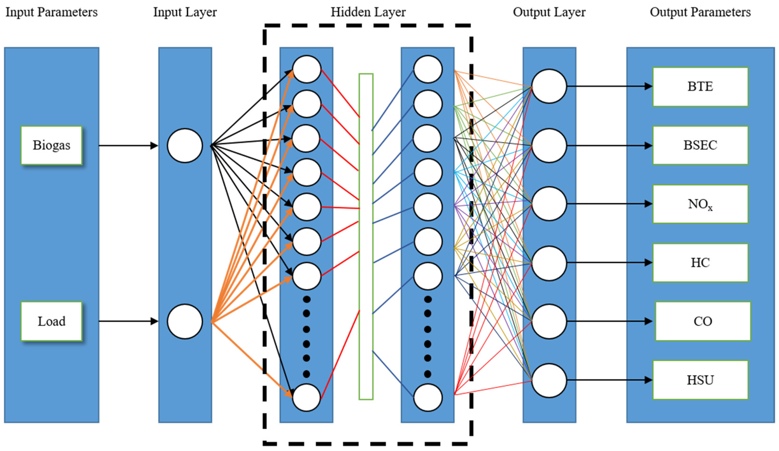
Artificial neural network model was developed by using Matlab R2018. Biogas flow rate and the load were the input for all the experimental trials used in the ANN model. Emission and performance data acquired during the experimental process was used as an output parameter in the model. ANN configuration diagram is shown in Figure 2.

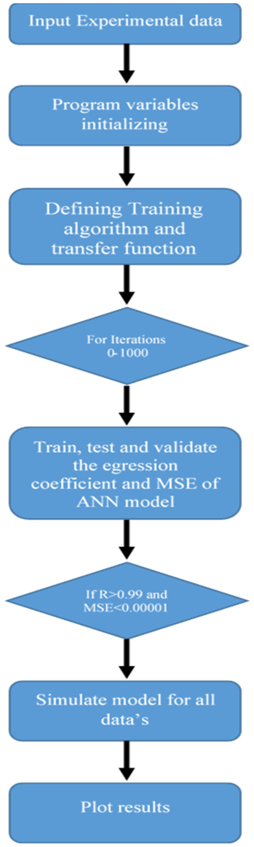
Artificial neural network model was trained in MATLAB R2018 by employing different training algorithms, functions, and changing the neurons in different layers. Tansig (Hyperbolic tangent sigmoid) and Logsig (logarithmic sigmoid) transfer functions were used in the layers of the model. Weights and bias were randomly chosen by MATLAB and initially the network executed 100 iterations. The minimum gradient was 10⁻⁷ and the stopping criteria for the network were 10,000 epochs [45].

To understand the output of the model, a simulation of all input data matching was carried out. The ANN model was evaluated by regression coefficient Equation (8), Mean square error Equation (9) by employing targets and outputs of the model:

$$\mathit{Regression} \mathit{Coefficient}=\sqrt{1-\left\{\frac{{\sum }_{i=1}^n{\left(T_i-O_i\right)}^2}{{\sum }_{i=1}^n{O}_i^2}\right\}},$$

(8)

$$\mathit{Mean} \mathit{Squared} \mathit{Error}=\frac{1}{n}\left\{{\sum }_{i=1}^n{\left(T_i-O_i\right)}^2\right\}.$$

(9)

The two statistical expressions value (R > 0.98 and MSE < 0.001) were used together to evaluate the model. After satisfying the iterations, it would be terminated. Figure 3 represents the developed ANN algorithm in MATLAB and the predicted data from the ANN model is given in

Table 5. Predicted data from the ANN model.

S.No	Bio Gas (kg/h)	BSEC (MJ/kWh) Predict
		20% Engine Load	40% Engine Load	60% Engine Load	80% Engine Load	100% Engine Load
1	1	38.51	27.53	22.28	20.00	18.27
2	2	41.44	29.17	22.77	20.97	18.48
3	3	44.81	30.79	23.06	21.93	18.97
4	4	47.74	32.95	23.56	22.49	19.56
5	5	50.50	35.03	24.73	23.04	20.17
6	6	53.51	37.04	26.10	23.84	20.86
7	7	56.50	38.95	27.60	24.54	21.61
8	8	61.10	40.91	29.02	25.28	22.20
9	9	65.25	43.07	30.19	26.02	22.71
10	10	69.51	45.10	31.08	26.75	23.11
11	11	72.56	46.62	33.55	27.44	23.36
12	12	75.49	48.78	34.05	27.99	23.95
13	13	78.25	50.87	35.22	28.54	24.56
14	14	81.26	52.88	36.59	29.34	25.26
15	15	84.26	54.78	38.09	30.04	26.00
S.No	Bio Gas (kg/h)	Brake Thermal Efficiency (Predicted)
		20% Engine Load	40% Engine Load	60% Engine Load	80% Engine Load	100% Engine Load
1	1	8.57%	14.92%	18.79%	19.93%	21.99%
2	2	8.02%	14.59%	18.50%	19.95%	21.91%
3	3	7.49%	14.14%	18.11%	19.35%	21.49%
4	4	6.96%	13.68%	17.52%	18.99%	21.32%
5	5	6.45%	13.38%	16.75%	18.37%	20.86%
6	6	5.98%	13.06%	16.05%	17.70%	20.46%
7	7	5.54%	12.52%	15.47%	17.59%	20.12%
8	8	5.16%	11.86%	14.99%	17.25%	19.79%
9	9	4.92%	11.51%	14.43%	16.81%	19.51%
10	10	4.75%	11.29%	13.87%	16.38%	19.18%
11	11	4.46%	11.04%	13.37%	15.85%	18.83%
12	12	4.08%	11.06%	12.89%	15.52%	18.50%
13	13	3.84%	10.55%	12.33%	15.08%	18.22%
14	14	3.66%	9.85%	11.77%	14.65%	17.89%
15	15	3.38%	9.48%	11.27%	14.12%	17.54%
S.No	Bio Gas (kg/h)	NOx (g/kWh) Predict
		20% Engine Load	40% Engine Load	60% Engine Load	80% Engine Load	100% Engine Load
1	1	42.78	35.26	26.31	20.55	14.40
2	2	41.54	33.59	24.66	19.72	13.69
3	3	39.51	32.11	23.39	18.87	13.01
4	4	37.39	30.20	22.40	17.89	12.26
5	5	35.78	28.35	21.49	17.06	11.41
6	6	34.41	26.56	20.48	16.44	10.52
7	7	32.94	24.82	19.44	15.77	9.64
8	8	31.47	23.29	18.98	14.94	8.44
9	9	29.65	22.15	18.20	14.01	7.09
10	10	26.49	20.70	17.21	13.15	6.02
11	11	25.52	18.45	15.68	12.42	5.56
12	12	24.16	16.67	14.67	11.80	4.68
13	13	22.68	14.93	13.63	11.14	3.79
14	14	21.21	13.40	13.17	10.31	2.60
15	15	19.40	12.26	12.39	9.38	1.23
S.No	Bio Gas (kg/h)	CO (% Vol) Predicted
		20% Engine Load	40% Engine Load	60% Engine Load	80% Engine Load	100% Engine Load
1	1	0.312	0.119	0.061	0.090	0.170
2	2	0.320	0.128	0.061	0.093	0.175
3	3	0.320	0.127	0.066	0.094	0.180
4	4	0.324	0.135	0.067	0.096	0.182
5	5	0.330	0.137	0.070	0.098	0.185
6	6	0.331	0.140	0.071	0.100	0.190
7	7	0.337	0.142	0.073	0.101	0.193
8	8	0.340	0.147	0.075	0.103	0.196
9	9	0.345	0.150	0.076	0.106	0.199
10	10	0.346	0.155	0.078	0.107	0.205
11	11	0.350	0.159	0.081	0.110	0.211
12	12	0.353	0.162	0.086	0.112	0.212
13	13	0.357	0.167	0.087	0.113	0.217
14	14	0.362	0.176	0.090	0.115	0.221
15	15	0.367	0.184	0.092	0.117	0.226
S.No	Bio Gas (kg/h)	HC (g/kWh)
		20% Engine Load	40% Engine Load	60% Engine Load	80% Engine Load	100% Engine Load
1	1	1.18	0.78	0.66	0.47	0.28
2	2	1.32	0.85	0.70	0.54	0.28
3	3	1.42	0.92	0.76	0.58	0.28
4	4	1.56	0.99	0.78	0.60	0.28
5	5	1.65	1.05	0.77	0.67	0.29
6	6	1.77	1.09	0.80	0.73	0.30
7	7	1.87	1.17	0.86	0.77	0.32
8	8	1.95	1.24	0.89	0.78	0.34
9	9	2.00	1.29	0.95	0.79	0.37
10	10	2.09	1.35	0.98	0.83	0.38
11	11	2.20	1.42	1.00	0.87	0.39
12	12	2.29	1.47	1.03	0.93	0.41
13	13	2.41	1.51	1.09	0.98	0.43
14	14	2.51	1.59	1.12	1.02	0.45
15	15	2.59	1.66	1.18	1.08	0.47
S.No	Bio Gas (kg/h)	Smoke Opacity (% HSU)Predict
		20% Engine Load	40% Engine Load	60% Engine Load	80% Engine Load	100% Engine Load
1	1	15.75%	23.87%	29.89%	36.12%	44.93%
2	2	15.14%	23.41%	28.03%	34.25%	44.21%
3	3	14.54%	22.97%	26.97%	32.01%	41.98%
4	4	13.86%	22.36%	25.78%	29.89%	40.78%
5	5	13.03%	21.38%	24.09%	28.69%	39.10%
6	6	11.98%	20.00%	22.03%	28.00%	37.90%
7	7	10.77%	18.50%	20.46%	27.00%	36.40%
8	8	9.77%	16.84%	19.91%	25.85%	34.86%
9	9	9.30%	15.85%	19.19%	24.90%	33.34%
10	10	9.13%	14.55%	16.90%	23.91%	31.80%
11	11	8.11%	13.99%	15.75%	21.90%	30.10%
12	12	7.55%	13.43%	15.19%	21.10%	28.89%
13	13	6.99%	12.87%	14.47%	20.15%	27.40%
14	14	6.43%	12.31%	13.92%	19.06%	25.85%
15	15	5.78%	11.73%	12.77%	18.11%	24.33%

.

7. Results and Discussion

The model was trained with different algorithms and training functions, but the best training algorithm was Levenberge Marquardt and the training function was Tansig (Hyperbolic tangent sigmoid). The Logsig (logarithmic sigmoid) showed the best result with (R > 0.98) and (MSE < 0.001). The best model was trained by evaluating the mean square error and regression coefficient.

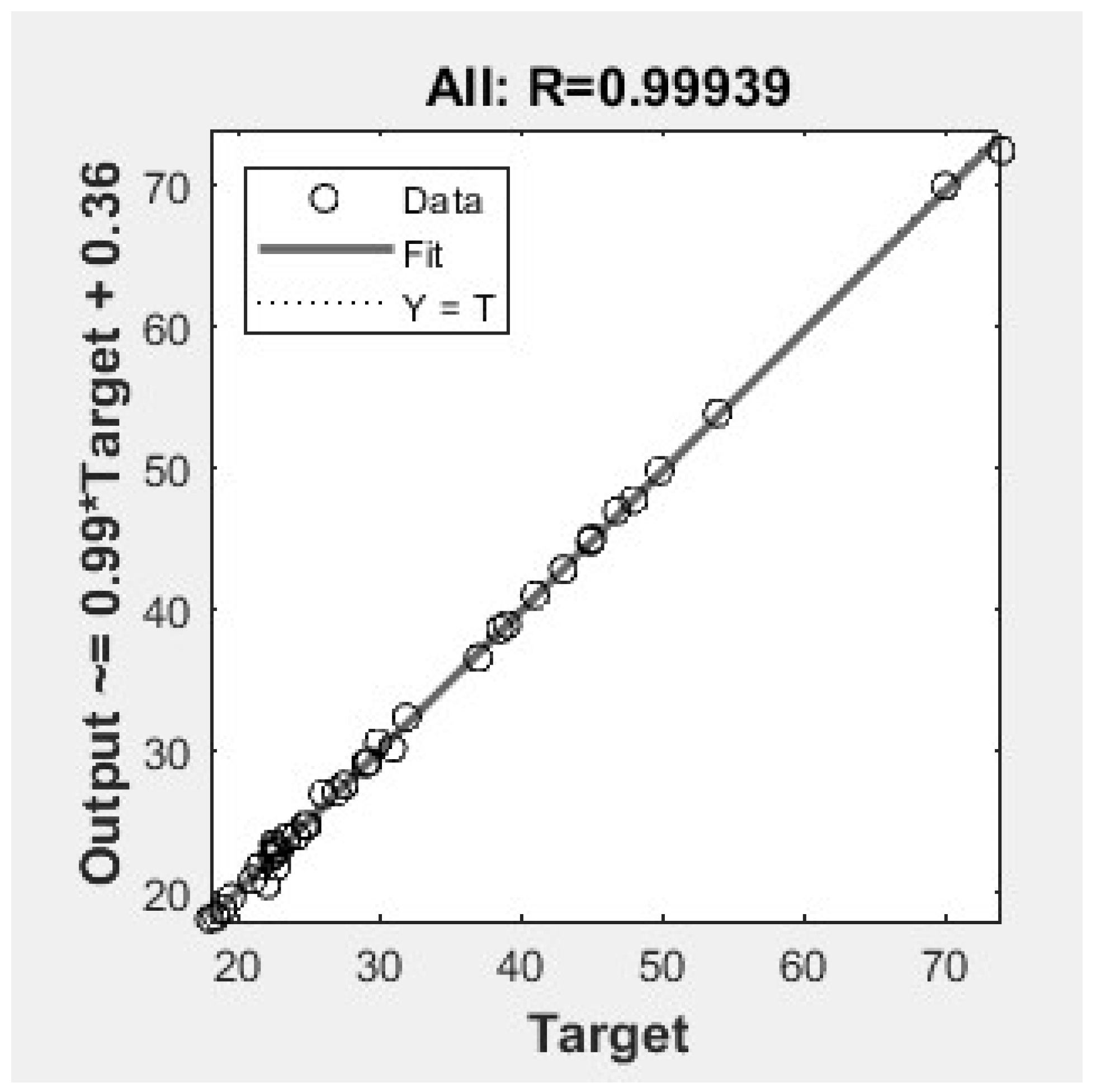
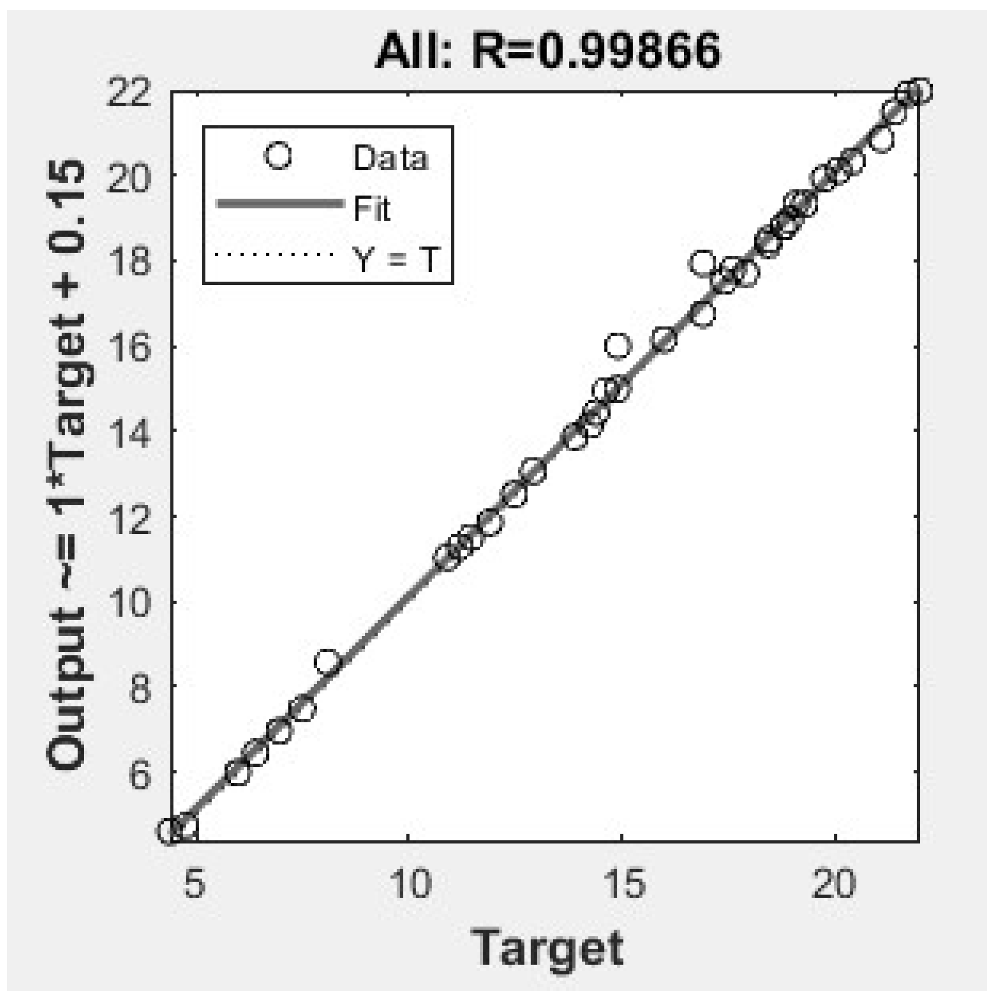
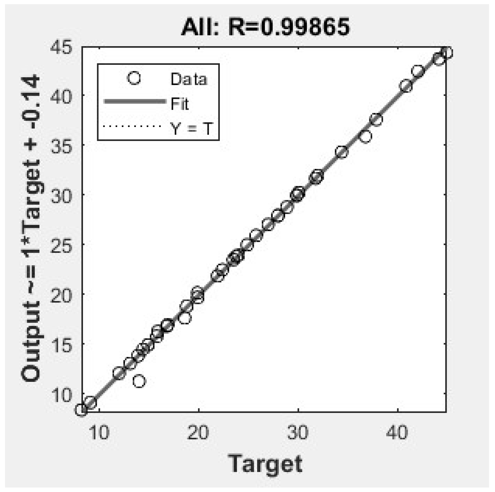
ANN predictions were used for the experimental values with regression coefficient and predictions. ANN predictions were matched with the actual data. Regression coefficient for emission for BSEC, BTE, NO_x, CO, HC and smoke opacity were 0.99939, 0.99866, 0.99699, 0.99942, 0.99706, and 0.99865 respectively.

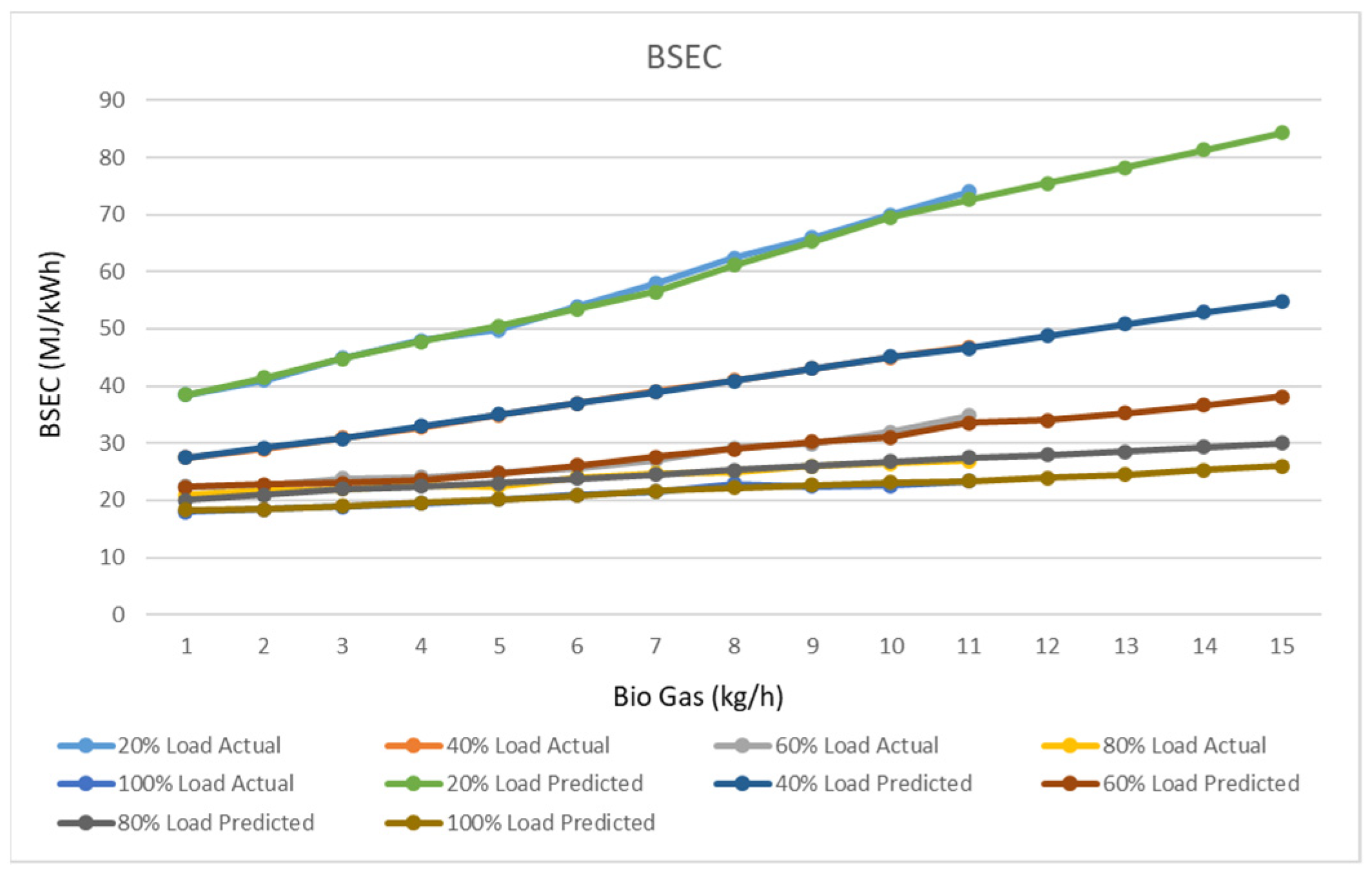
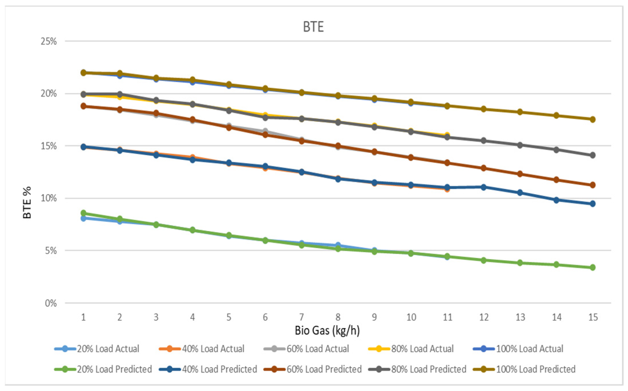
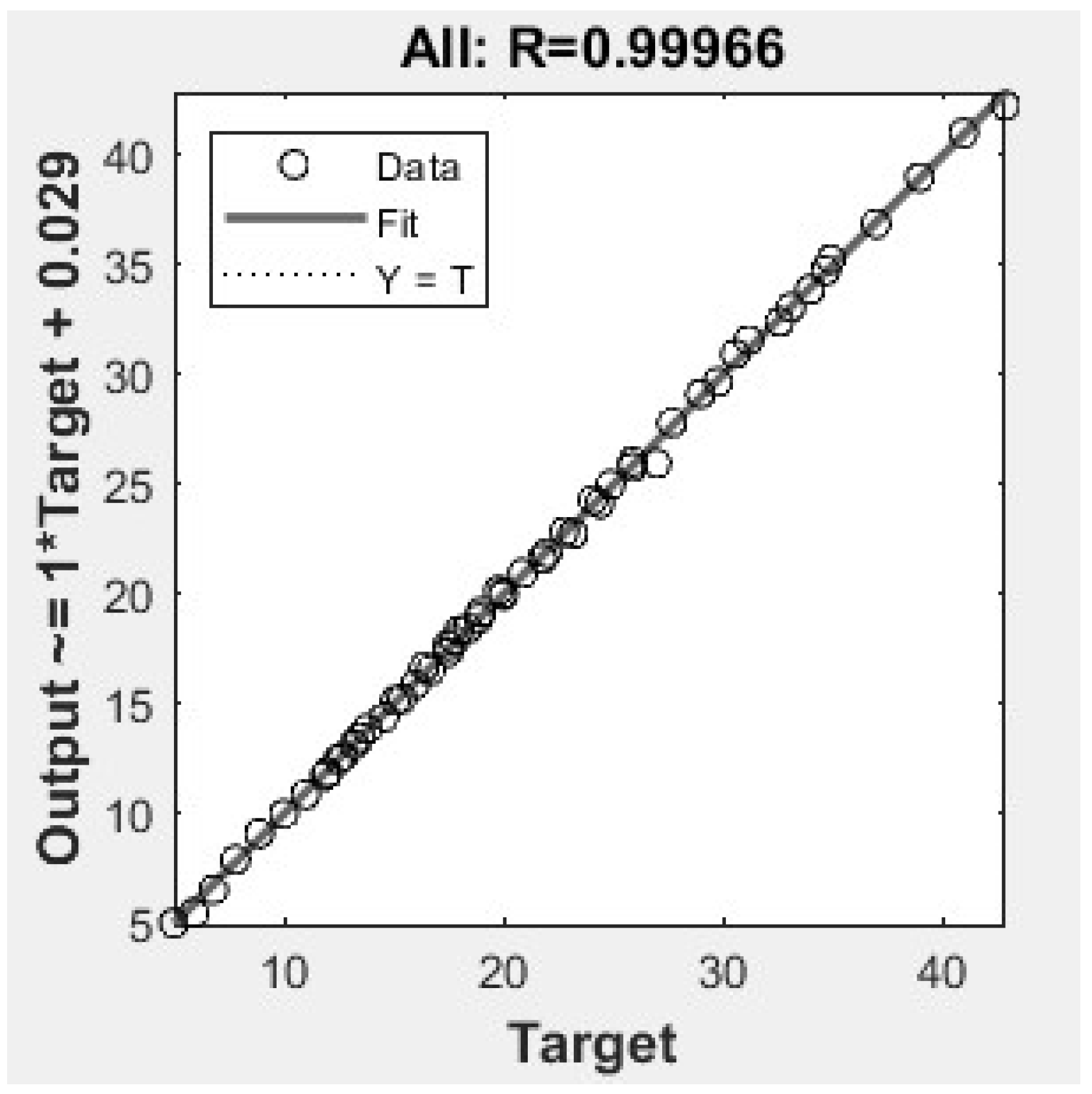
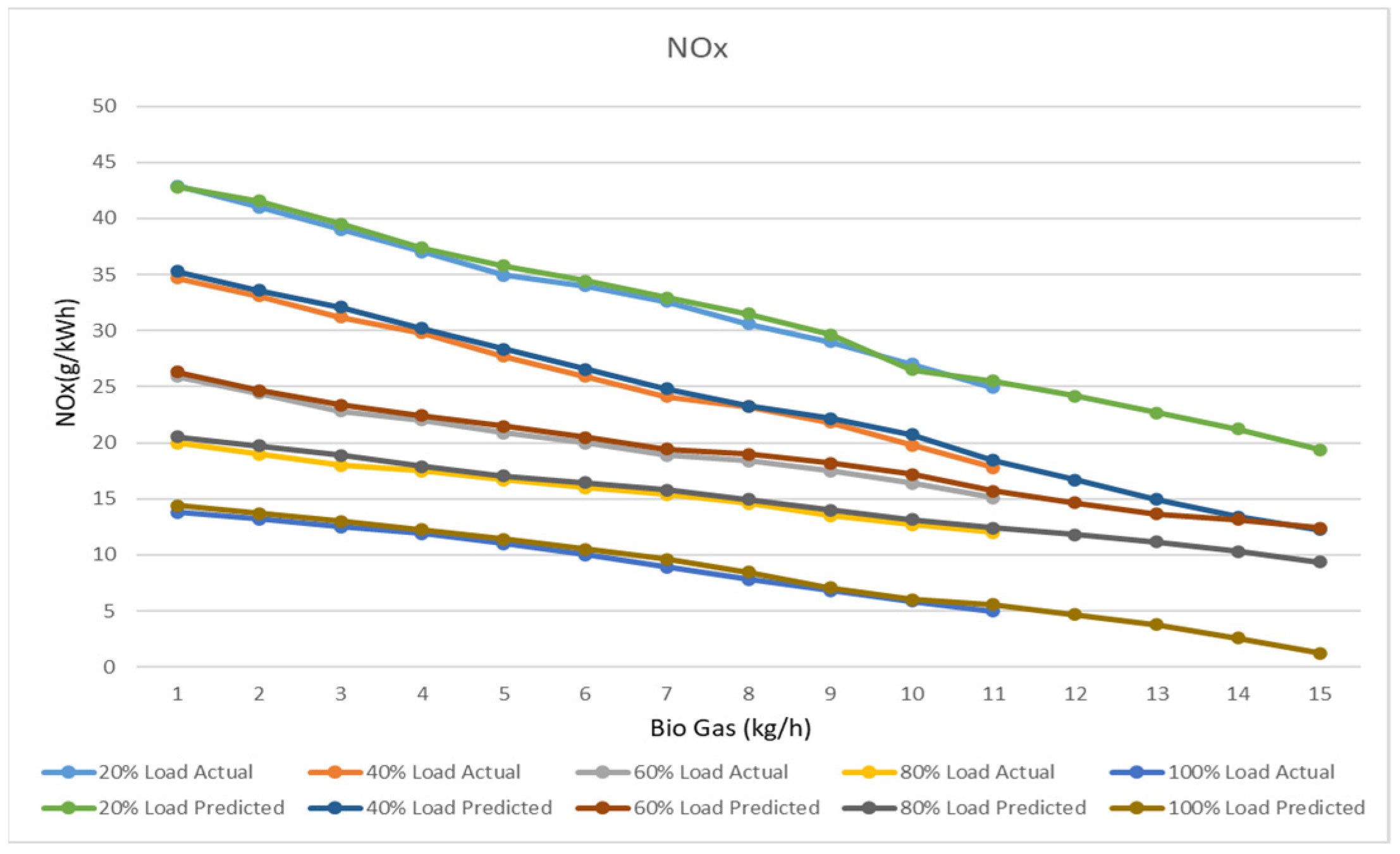
Figure 4 shows the accuracy of the training data, validation of the data, and test data. The closeness of data points with the Fit line shows that the accuracy of the predicted data and the regression coefficient (R = 0.99939) will be higher. The variation of BSEC at different engine loads is given in Figure 5. From the study, it is clear that BSEC was the highest and as we increase the flow of biogas from 1 kg/h to 15 kg/h, the BSEC increases linearly. At 100% engine load, BSEC was the lowest. The predicted values of BSEC at 20% load 1 kg/h biogas was 38.51 MJ/kWh, whereas at 15 kg/h BSEC was 84.26 MJ/kWh. As the engine load was increased, the BSEC decreased. BSEC at 100% engine load at 1 kg/h was 18.27 MJ/kWh. By increasing the biogas to 15 kg/h, the BSEC increased to 26.00 MJ/kWh. It can be concluded that the increase of biogas flow rate resulted in an overall lower heating value. From the figure, the maximum value was obtained for 20% engine load at 15 kg/h biogas mass flow rate. Figure 6 shows the regression coefficient (R = 0.99866) for BTE predictions for the accuracy of the training data, validation of the data, and test data. A variation of BTE with the variation of the mass flow rate of biogas at different engine loads is given in Figure 7. From the figure, it is clear that BTE is lower at 20% engine load, whereas at higher engine load BTE also increases. At 20% engine load at 1 kg/h biogas mass flow rate, the value of BTE was 8.57% and on increasing the gas flow rate, the BTE reduced to 3.38%. The highest BTE was at 100% engine load at 1 kg/h biogas flow rate with 21.99% BTE. On increasing the flow rate, the BTE was reduced to 17.54% at 15 kg/h. It could be observed that upon increasing the engine load, BTE increased. It was because poor utilization of gaseous fuel mixture resulted in reduced BTE under dual fuel mode. Figure 8 shows the regression coefficient (R = 0.99966) for NO_x prediction. This shows how closely the training data and test data match closely with each other. Variation of NO_x with the variation in the mass flow rate of biogas at different engine loads is given in Figure 9. From the figure, it is clear that at a lower engine load, NO_x emission is higher. At 20% engine load and 1 kg/h biogas flow rate, the value of NO_x was 42.78 g/kWh and on increasing the gas flow rate, it reduced to 19.40 g/kWh. At 100% engine load and 1 kg/h biogas flow rate, NO_x was 14.40 g/kWh and on increasing the flow rate further, it reduces to 1.23 g/kWh. Increasing the engine load reduces the NO_x. It further reduces on increasing the biogas flow rate in the engine. It could be justified as the use of biogas diminishes the harmful emissions.

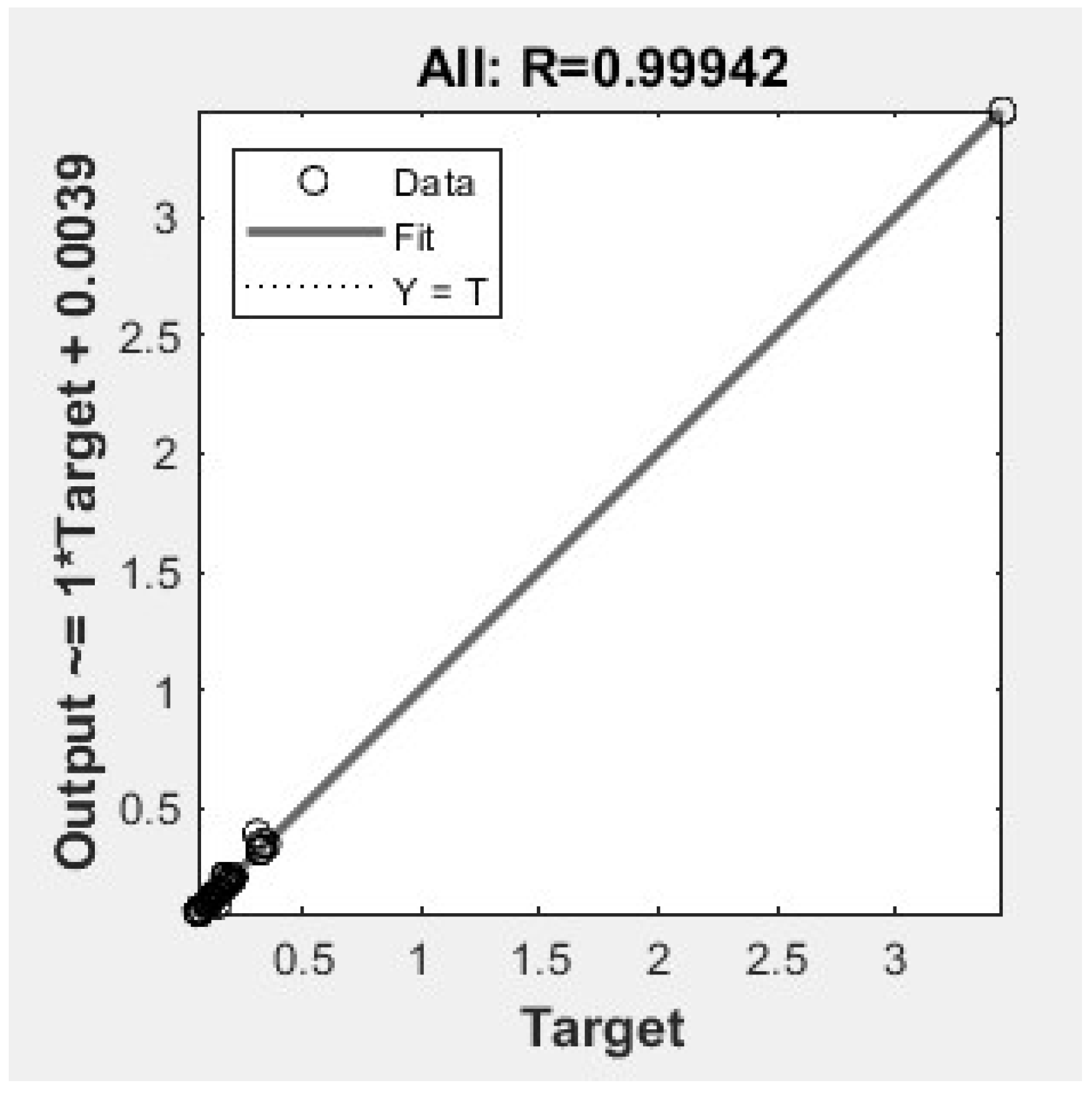
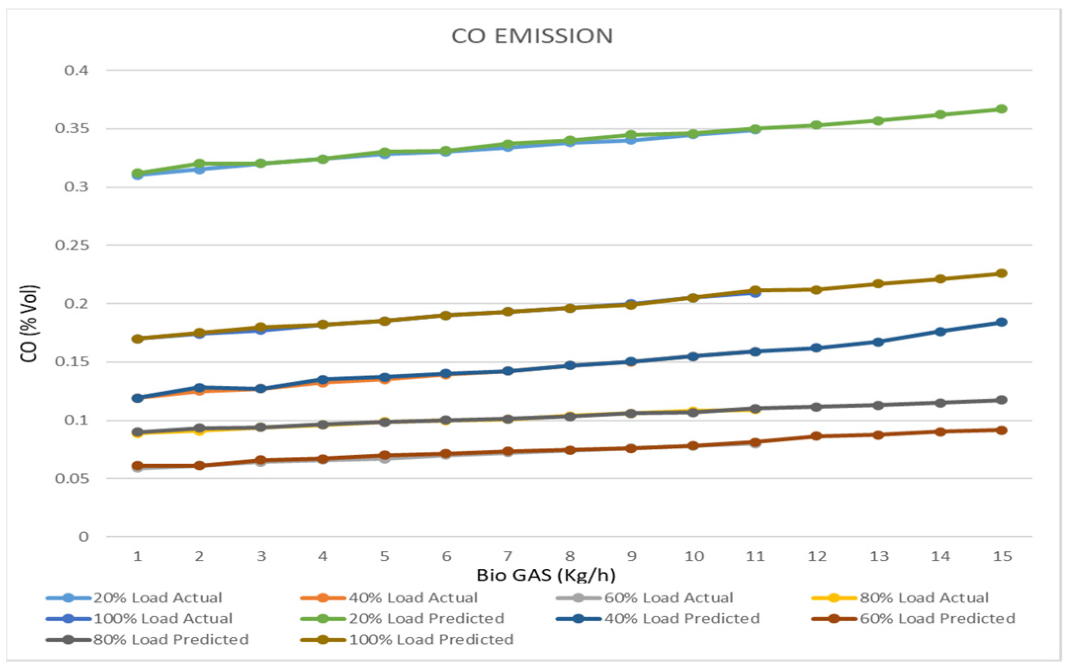
Figure 10 shows the regression coefficient of CO emission, i.e., R = 0.99942. CO emission increases with an increase in engine load and biogas flow rate. CO emission increases with a decrease in load and increase in biogas flow into the engine, as shown in Figure 11. At 20% engine load and 1 kg/h biogas flow rate, CO emission was 0.312% Vol, increasing the biogas flow rate to 15 kg/h increases the CO to 0.367% Vol. On increasing the engine load at 1 kg/h biogas flow rate, CO emission were 0.119% Vol, 0.061% Vol, 0.090% Vol, and 0.170% Vol, respectively for 40%, 60%, 80%, and 100% engine load. Increasing the mass flow rate of biogas in the engine decreases the oxygen supply in the engine, which leads to higher CO emissions.

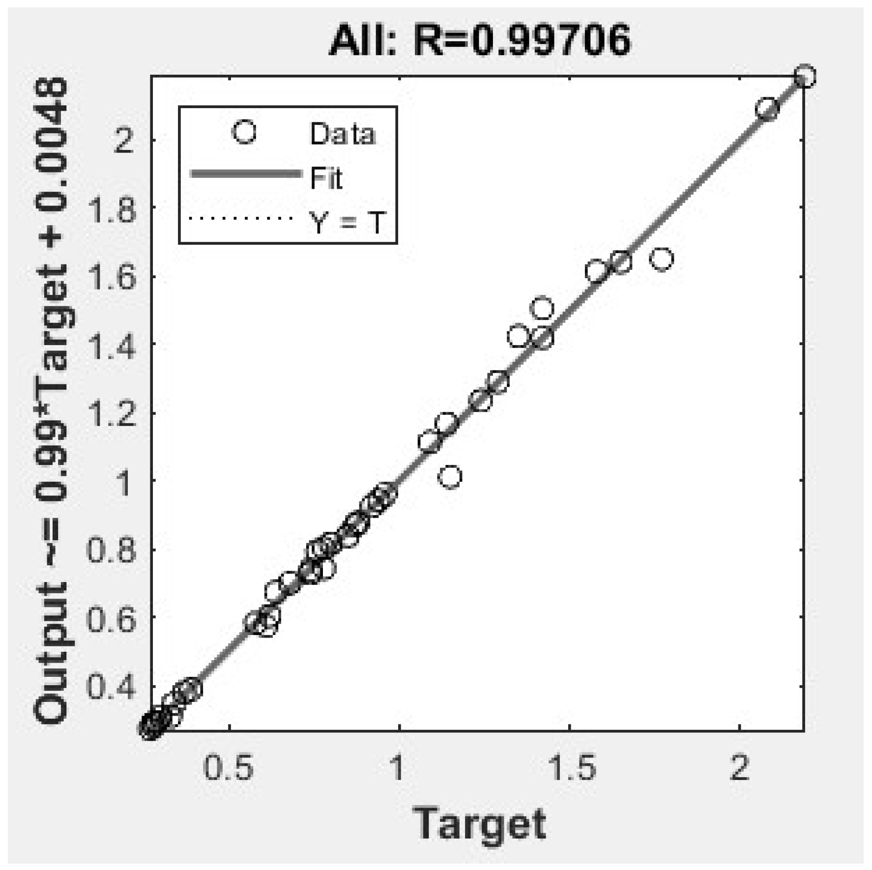
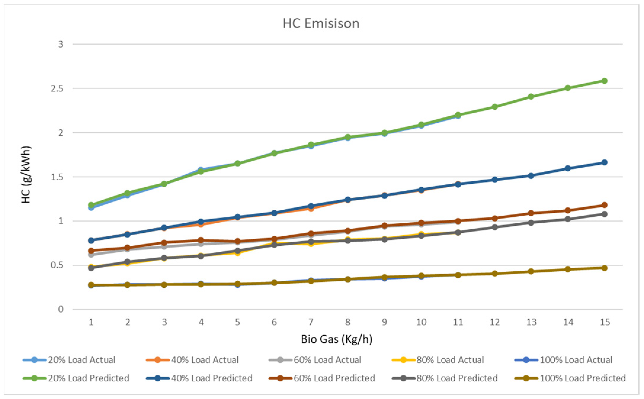
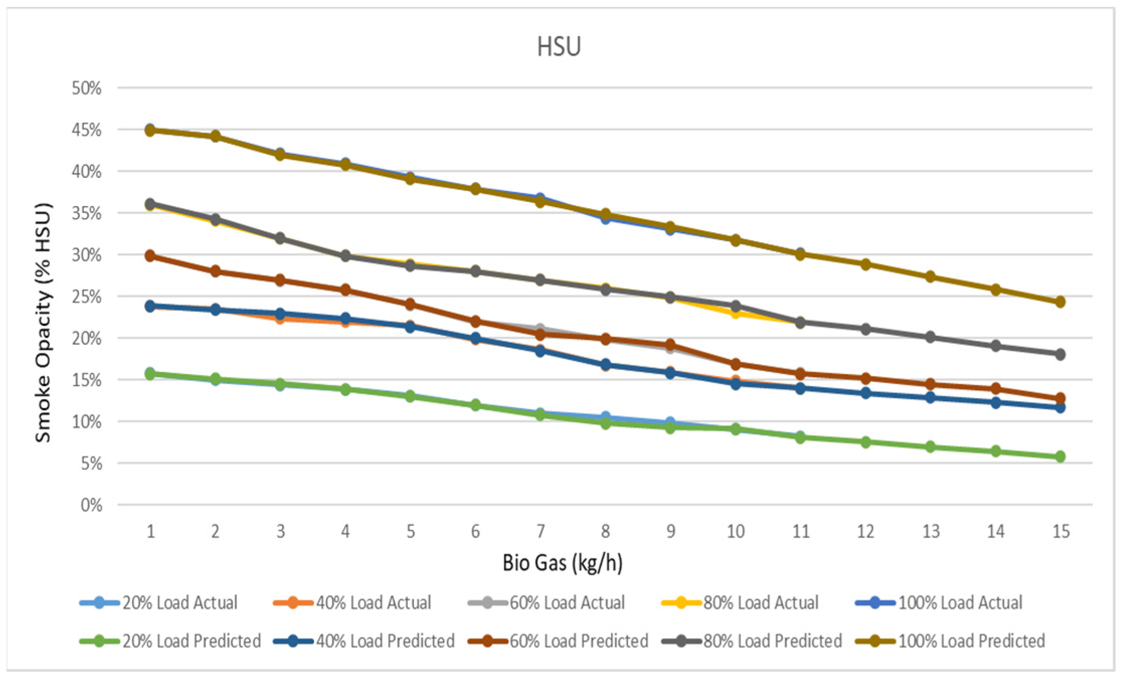
Figure 12 shows the regression coefficient (R = 0.99706) for HC prediction. Variation of HC with the variation of the mass flow rate of biogas at different engine loads is given in Figure 13. From the figure, it is clear that HC emissions are lower at lower engine loads. At 20% engine load and 1 kg/h biogas flow rate, the value of HC was 1.18 g/kWh and on increasing the gas flow rate it increases to 2.59 g/kWh. At 100% engine load and 1 kg/h biogas flow rate, the HC was 0.28 g/kWh and on increasing the flow rate further, it increases to 0.47 g/kWh. Increasing the engine load reduces the HC. It increases by increasing the biogas flow rate in the engine. At 15 kg/h biogas flow rate, HC was 2.59, 1.66, 1.18, 1.08, and 0.47 g/kWh for 20%, 40%, 60%, 80%, and 100% engine load, respectively. An increase in HC with an increase in biogas flow rate could be justified by the lower flame velocity of biogas. The regression coefficient for smoke opacity was 0.099865, as shown in Figure 14. Variation of smoke opacity with the variation of the mass flow rate of biogas at different engine loads is given in Figure 15. From the figure, it is clear that smoke opacity increases the engine load. At 20% engine load and 1 kg/h biogas flow rate, smoke opacity was 15.75%. Increasing the biogas flow rate to 15 kg/h reduces the smoke opacity to 5.78%. At 100% engine load, 1 kg/h biogas flow rate smoke opacity was 44.93% and increasing the biogas flow reduced the smoke opacity to 24.33%. A decrease in smoke opacity with an increase in biogas is because of the absence of aromatic compounds in the biogas composition.

8. Conclusions

Performance and emission characteristics of a dual-fueled compression ignition engine were predicted using an artificial neural network, by varying the mass flow rate of biogas. Biogas is a clean fuel (obtained by anaerobic digestion from agricultural wastes) and a better alternative to conventional fuels, which reduces the NO_x emissions gases without a major change in the existing diesel engine. ANN helped in predicting the performance and emission characteristics of the CI engine at different biogas mass flow rates. The comparative study shows that the experimental results are clearly identical to the ANN results. Based on the study it was noted that:

• ANN model was trained using the Levenberge Marquardt algorithm and training function was Tansig (Hyperbolic tangent sigmoid) and Logsig (logarithmic sigmoid).
• ANN model was evaluated on the basis of the regression coefficient(R > 0.98) and Mean squared error (MSE < 0.0001).
• BSEC was highest at 20% engine load and as we increase the flow of biogas from 1 kg/h to 15 kg/h BSEC increases linearly. At 20% engine load and 1 kg/h biogas flowrate, BSEC was 38.51 MJ/kWh, whereas at 100% load it was 18.27 MJ/kWh. Increasing the biogas flow rate increases the BSEC to 84.26 MJ/kWh and 26.00 MJ/kWh for 20% engine load and 100% engine load, respectively. It could be justified as an increase in biogas resulted in a lower heating value.
• BTE at 20% and 100% engine load and 1 kg/h biogas flow rate was 8.57% and 21.99%. On increasing the gas flow rate to 15 kg/h, BTE was reduced to 3.38% and 17.54%. Poor utilization of gaseous fuel may be blamed for lower BTE under dual fuel mode.
• NO_x prediction showed that at 20% engine load and 1 kg/h biogas flow rate, the value of NOx was 42.78 g/kWh and on increasing the gas flow rate, it reduced to 19.40 g/kWh. At 100% engine load and 1 kg/h biogas flow rate, NOx was 14.40 g/kWh and on increasing the flow rate further, it reduces to 1.23 g/kWh.
• CO emission increases with a decrease in load and an increase in biogas flow into the engine. Biogas decreases the oxygen supply in the engine, which leads to higher CO emissions.
• Prediction showed that the trend of HC was similar to that of the experimental value. Increasing the engine load reduces the HC and it increases on increasing the biogas flow rate in the engine. The lower flame velocity of biogas was the reason for the increase in HC.
• The absence of aromatic compounds in the biogas decreased the smoke opacity with an increase in biogas mass flow rate.

It could be concluded that this study helps in understanding the effect of dual fuel (diesel-biogas) combustion under different load conditions of the engine with the help of ANN, which could be a substitute fuel and help to protect the environment.

References

- Goga, G.; Chauhan, B.S.; Mahla, S.K.; Dhir, A.; Cho, H.M. Combined impact of varying biogas mass flow rate and rice bran methyl esters blended with diesel on a dual-fuel engine. Energy Sources Part A 2021, 43, 120–132. [Google Scholar] [CrossRef]
- Rosha, P.; Mohapatra, S.K.; Mahla, S.K.; Cho, H.M.; Chauhan, B.S.; Dhir, A. Effect of compression ratio on combustion, performance, and emission characteristics of compression ignition engine fueled with palm (B20) biodiesel blend. Energy 2019, 178, 676–684. [Google Scholar] [CrossRef]
- Mahla, S.K.; Ardebili, S.M.S.; Mostafaei, M.; Dhir, A.; Goga, G.; Chauhan, B.S. Multi-objective optimization of performance and emissions characteristics of a variable compression ratio diesel engine running with biogas-diesel fuel using response surface techniques. Energy Sources Part A 2020, 1–18. [Google Scholar] [CrossRef]
- Goga, G.; Chauhan, B.S.; Mahla, S.K.; Dhir, A.; Cho, H.M. Effect of varying biogas mass flow rate on performance and emission characteristics of a diesel engine fueled with blends of n-butanol and diesel. J. Therm. Anal. Calorim. 2020, 140, 2817–2830. [Google Scholar] [CrossRef]
- Goga, G.; Chauhan, B.S.; Mahla, S.K.; Cho, H.M. Performance and emission characteristics of diesel engine fuelled with rice bran biodiesel and n-butanol. Energy Rep. 2019, 5, 78–83. [Google Scholar] [CrossRef]
- Dimitrakopoulosa, N.; Giacomo, B.; Tunéra, M.; Tuneståla, P.; Di Blasio, G. Effect of EGR routing on efficiency and emissions of a PPC engine. Appl. Therm. Eng. 2019, 152, 742–750. [Google Scholar] [CrossRef]
- Singh, R.; Dhir, A.; Mohapatra, S.K.; Mahla, S.K. Dry reforming of methane using various catalysts in the process. Biomass Convers. Biorefinery 2020, 10, 567–587. [Google Scholar] [CrossRef]
- Bora, J.B.; Saha, U.K. Comparative assessment of a biogas run dual fuel diesel engine with rice bran oil methyl ester, pongamia oil methyl ester and palm oil methyl ester as pilot fuels. Renew. Energy 2015, 81, 490–498. [Google Scholar] [CrossRef]
- Barik, D.; Murugan, S. Investigation on Performance and Exhaust Emissions Characteristics of a DI Diesel Engine Fueled with Karanja Methyl Ester and Biogas in Dual Fuel Mode; SAE Technical Paper: Warrendale, PA, USA, 2014; pp. 1–9. [Google Scholar] [CrossRef]
- Porpatham, E.; Ramesh, A.; Nagalingam, B. Effect of compression ratio on the performance and combustion of a biogas fuelled spark ignition engine. Energy Convers. Manag. 2012, 95, 247–256. [Google Scholar] [CrossRef]
- Ali, M.O.; Rizalman, M.; Gholamhassan, N.; Talal, Y. Optimization of biodiesel-diesel blended fuel properties and engine performance with ether additive using statistical analysis and response surface methods. Energies 2015, 8, 14136–14150. [Google Scholar] [CrossRef] [Green Version]
- Namasivayam, A.M.; Korakianitis, T.; Crookes, R.J.; Bob-Manuel, K.D.H.; Olsen, J. Biodiesel, emulsified biodiesel and dimethyl ether as pilot fuels for natural gas fuelled engines. Appl. Energy 2010, 87, 769–778. [Google Scholar] [CrossRef]
- Gaikwad, M.S.; Jadhav, K.M.; Kolekar, A.H.; Chitragar, P.R. Combustion characteristics of biomethane–diesel dual-fueled CI engine with exhaust gas recirculation. Biofuels 2018, 12, 369–379. [Google Scholar] [CrossRef]
- Sayin Kul, B.; Kahraman, A. Energy and Exergy Analyses of a Diesel Engine Fuelled with Biodiesel-Diesel Blends Containing 5% Bioethanol. Entropy 2016, 18, 387. [Google Scholar] [CrossRef]
- Monsalve-Serrano, J.; Belgiorno, G.; Di Blasio, G.; Guzmán-Mendoza, M. 1D Simulation and Experimental Analysis on the Effects of the Injection Parameters in Methane–Diesel Dual-Fuel Combustion. Energies 2020, 13, 3734. [Google Scholar] [CrossRef]
- Piechota, G.; Iglinski, B. Biomethane in Poland—Current Status, Potential, Perspective and Development. Energies 2021, 14, 1517. [Google Scholar] [CrossRef]
- Murano, R.; Maisano, N.; Selvaggi, R.; Pappalardo, G.; Pecorino, B. Critical Issues and Opportunities for Producing Biomethane in Italy. Energies 2021, 14, 2431. [Google Scholar] [CrossRef]
- Mahla, S.K.; Dhir, A.; Gill, J.B.; Cho, H.M.; Lim, H.C. Influence of EGR on the simultaneous reduction of NOx-Smoke opacity trade-off under CNG-Biodiesel dual fuel engine. Energy 2018, 152, 303–312. [Google Scholar] [CrossRef]
- Zepter, J.M.; Engelhardt, J.; Gabderakhmanova, T.; Marinelli, M. Empirical Validation of a Biogas Plant Simulation Model and Analysis of Biogas Upgrading Potentials †. Energies 2021, 14, 2424. [Google Scholar] [CrossRef]
- Scarlat, N.; Dallemand, J.-F.; Fahl, F. Biogas: Developments and perspectives in Europe. Renew. Energy 2018, 129, 457–472. [Google Scholar] [CrossRef]
- Ryckebosch, E.; Drouillon, M.; Vervaeren, H. Techniques for transformation of biogas to biomethane. Techniques for transformation of biogas to biomethane. Biomass Bioenergy 2018, 129, 457–472. [Google Scholar]
- Palash, S.M.; Masjuki, H.H.; Kalam, M.A.; Atabani, A.E.; Fattah, I.R.; Sanjid, A. Biodiesel production, characterization, diesel engine performance, and emission characteristics of methyl esters from aphanamixispolys-tachya oil of bangladesh. Energy Convers. Manag. 2015, 91, 149–157. [Google Scholar] [CrossRef] [Green Version]
- Barik, D.; Murugan, S. Effects of diethyl ether (DEE) injection on combustion performance and emission characteristics of Karanja methyl ester (KME)–biogas fueled dual fuel diesel engine. Fuel 2016, 164, 286–296. [Google Scholar] [CrossRef]
- Jingura, R.M.; Matengaifa, R. Optimization of biogas production by anaerobic digestion for sustainable energy development in Zimbabwe. Renew. Sustain. Energy Rev. 2009, 13, 1116–1120. [Google Scholar] [CrossRef]
- Mahla, S.K.; Das, L.M.; Babu, M.K.G. Effect of EGR on performance and emission characteristics of natural gas fueled diesel engine. Jordan J. Mech. Ind. Eng. 2010, 4, 523–530. [Google Scholar]
- Barik, D.; Murugan, S. Performance and Emission Characteristics of a Biogas Fueled DI Diesel Engine; SAE Technical Paper: Warrendale, PA, USA, 2013; pp. 1–11. [Google Scholar] [CrossRef]
- Yoon, S.H.; Lee, C.K. Experimental investigation on the combustion and exhaust emission characteristics of biogas—Biodiesel dual-fuel combustion in a CI engine. Fuel Process Technol. 2011, 92, 992–1000. [Google Scholar] [CrossRef]
- Barik, D.; Murugan, S. Simultaneous reduction of NOx and smoke in a dual fuel DI diesel engine. Energy Convers. Manag. 2014, 84, 217–226. [Google Scholar] [CrossRef]
- Goga, G.; Chauhan, B.S.; Mahla, S.K.; Cho, H.M.; Dhir, A.; Lim, H.C. Properties and characteristics of various materials used as biofuels: A review. Mater. Today Proc. 2018, 5, 28438–28445. [Google Scholar] [CrossRef]
- Duc, P.H.; Wattanavichien, K. Study on biogas premixed charge diesel dual fuelled engine. Energy Convers. Manag. 2007, 48, 2286–2308. [Google Scholar] [CrossRef]
- Mahla, S.K.; Singla, V.; Sandhu, S.S. Performance and emissions characteristics of compression ignition engine fuelled with biogas-diesel under dual fuel mode. Environ. Sci. Pollut. Res. 2018, 25, 9722–9729. [Google Scholar] [CrossRef] [PubMed]
- Mahla, S.K.; Dhir, A. Performance and emission characteristics of CNG-fuelled compression ignition engine with Ricinus communis methyl ester as pilot fuel. Environ. Sci. Pollut. Res. 2019, 26, 775–785. [Google Scholar] [CrossRef] [PubMed]
- Bora, B.J.; Saha, U.K. Experimental evaluation of a rice bran biodiesel—Biogas run dual fuel diesel engine at varying compression ratios. Renew. Energy 2016, 67, 782–790. [Google Scholar] [CrossRef]
- Karthic, S.V.; Kumar, M.S. Predicting the performance and emission characteristics of a Mahua oil-hydrogen dual fuel engine using artificial neural networks. Energy Sources Part A 2020, 42, 2891–2910. [Google Scholar]
- Gul, M.; Shah, A.N.; Aziz, U.; Husnain, N.; Mujtaba, M.A.; Kousar, T.; Ahmad, R.; Hanif, M.F. Grey-Taguchi and ANN based optimization of a better performing low-emission diesel engine fueled with biodiesel. Energy Sources Part A 2019, 1–14. [Google Scholar] [CrossRef]
- Kumar, S. Process parameter assessment of biodiesel production from a Jatropha—Algae oil blend by response surface methodology and artificial neural network. Energy Sources Part A 2017, 39, 2119–2125. [Google Scholar] [CrossRef]
- Samuel, O.D.; Okwu, M.O. Comparison of Response Surface Methodology (RSM) and Artificial Neural Network (ANN) in modelling of waste coconut oil ethyl esters production. Energy Sources Part A 2018, 41, 1049–1061. [Google Scholar] [CrossRef]
- Calik, A.; Yildirim, S.; Tosun, E.; Uluocak, I.; Avsar, E. Artificial intelligence techniques for the vibration, noise, and emission characteristics of a hydrogen-enriched diesel engine. Energy Sources Part A 2019, 41, 2194–2206. [Google Scholar]
- Najafi, B.; Akbarian, E.; Lashkarpour, S.M.; Aghbashlo, M.; Ghaziaskar, H.S.; Tabatabaei, M. Modeling of a dual fueled diesel engine operated by a novel fuel containing glycerol triacetate additive and biodiesel using artificial neural network tuned by genetic algorithm to reduce engine emissions. Energy 2019, 168, 1128–1137. [Google Scholar] [CrossRef]
- Sahoo, B.B.; Sahoo, N.; Saha, U.K. Effect of engine parameters and type of gaseous fuel on the performance of dual-fuel gas diesel engines—A critical review. Renew. Sustain. Energy Rev. 2009, 13, 1151–1184. [Google Scholar] [CrossRef]
- Barik, D.; Murugan, S. Assessment of sustainable biogas production from de-oiled seed cake of karanja-an organic industrial waste from biodiesel industries. Fuel 2015, 148, 25–31. [Google Scholar] [CrossRef]
- Holman, J.P. Experimental Methods for Engineers, 8th ed.; McGraw-Hill Publishers: New York, NY, USA, 2012; pp. 60–163. [Google Scholar]
- Dey, S.; Reang, N.R.; Majumder, A.; Deb, M.; Das, P.K. A hybrid ANN-Fuzzy approach for optimization of engine operating parameters of a CI engine fueled with diesel-palm biodiesel-ethanol blend. Energy 2020, 202, 1–17. [Google Scholar] [CrossRef]
- Işcan, B. ANN modeling for justification of thermodynamic analysis of experimental applications on combustion parameters of a diesel engine using diesel and safflower biodiesel fuels. Fuel 2020, 279, 118391. [Google Scholar] [CrossRef]
- Javed, S.; Murthy, Y.V.V.S.; Baig, R.U.; Rao, D.P. Development of ANN model for prediction of performance and emission characteristics of hydrogen dual fueled diesel engine with Jatropha Methyl Ester biodiesel blends. J. Nat. Gas Sci. Eng. 2015, 26, 549–557. [Google Scholar] [CrossRef]
- Chakraborty, G.; Chakraborty, B. A novel normalization technique for unsupervised learning in ANN. IEEE Trans. Neural Netw. 2000, 11, 253–257. [Google Scholar] [CrossRef] [PubMed]
- Taghavifara, H.; Taghavifarb, H.; Mardania, A.; Mohebbia, A.; Khalilarya, S. A numerical investigation on the wall heat flux in a DI diesel engine fueled with n-heptane using a coupled CFD and ANN approach. Fuel 2015, 140, 227–236. [Google Scholar] [CrossRef]
- Çay, Y.; Çiçek, A.; Kara, F.; Sağiroğlu, S. Prediction of engine performance for an alternative fuel using artificial neural network. Appl. Therm. Eng. 2012, 37, 217–225. [Google Scholar] [CrossRef]
Figure 1.
Experimental setup block diagram.
Figure 2.
Artificial neural network structure for experiment.
Figure 3.
ANN model flowchart.
Figure 4.
Accuracy of the target and output data of BSEC using a Regression Coefficient metric.
Figure 5.
Effect on BSEC by change in engine load.
Figure 6.
Accuracy of the target and output data of BTE using a Regression Coefficient metric.
Figure 7.
Effect on BTE with change in engine load.
Figure 8.
Accuracy of the target and output data of NOx using a Regression Coefficient metric.
Figure 9.
Effect on NOx with change in engine load.
Figure 10.
Accuracy of the target and output data of CO using a Regression Coefficient metric.
Figure 11.
Effect on CO with change in engine load.
Figure 12.
Accuracy of the target and output data of HC using a Regression Coefficient metric.
Figure 13.
Effect on HC with change in engine load.
Figure 14.
Accuracy of the target and output data of smoke opacity using a Regression Coefficient metric.
Figure 15.
Effect on smoke opacity with change in engine load.