Article

A PROMETHEE Multiple-Criteria Approach to Combined Seismic and Flood Risk Assessment at the Regional Scale

1
Department of Engineering, University of Ferrara, 44122 Ferrara, Italy
2
Department of Environmental and Prevention Sciences, University of Ferrara, 44122 Ferrara, Italy
3
Faculty of Civil Engineering, Architecture and Geodesy, University of Split, 21000 Split, Croatia
4
OGS, Istituto Nazionale di Oceanografia e di Geofisica Sperimentale, Borgo Grotta Gigante 42/C, 34010 Sgonico, Italy
*
Author to whom correspondence should be addressed.
Appl. Sci. 2022, 12(3), 1527; https://doi.org/10.3390/app12031527
Submission received: 30 November 2021 / Revised: 26 January 2022 / Accepted: 27 January 2022 / Published: 31 January 2022
(This article belongs to the Special Issue Natural-Hazards Risk Assessment for Disaster Mitigation)

Abstract

:
Social vulnerability is deeply affected by the increase in hazardous events such as earthquakes and floods. Such hazards have the potential to greatly affect communities, including in developed countries. Governments and stakeholders must adopt suitable risk reduction strategies. This study is aimed at proposing a qualitative multi-hazard risk analysis methodology in the case of combined seismic and flood risk using PROMETHEE, a Multiple-Criteria Decision Analysis technique. The present case study is a multi-hazard risk assessment of the Ferrara province (Italy). The proposed approach is an original and flexible methodology to qualitatively prioritize urban centers affected by multi-hazard risks at the regional scale. It delivers a useful tool to stakeholders involved in the processes of hazard management and disaster mitigation.

1. Introduction

Many areas in Europe and worldwide are increasingly subjected to catastrophic events. These events intensify the exposure of these territories to multi-risk events and make societies more vulnerable to entangled risks [1,2,3,4,5,6,7]. Globalization and climate changes are the main culprits of these multi-risk dynamics. Globalization, indeed, makes countries closely linked and interdependent, so communities are not only vulnerable to local extreme events but also to those occurring outside their national territories. Climate change increases, among others, the frequency and intensity of extreme meteorological phenomena, hydrological and flood risk, as well as the risk of fires. The awareness of this worrying trend has determined the need for adequate tools to address and mitigate these risks, as well as information campaigns to foster resilience and coping capacity of communities [5,6,7].
Understanding risks involving vast inhabited areas is therefore paramount, particularly when assessing potential losses produced by a combination of multiple hazards. Hereafter, a hazard refers to the probability of occurrence in a specified period of a potentially damaging event of a given magnitude in a given area [8]. Total risk is a measure of the expected human (casualties, injuries) and economic (damage to property, activity disruption) losses due to adverse natural phenomena. Such a measure is assumed to be the product of hazard, vulnerability, and exposure instances [9]. Many areas on Earth are subjected to the effects of coexisting multiple hazards, among which floods [3,8] and earthquakes are some of the most widespread [5,6,7]. Though inhabited environments are affected by multiple hazardous processes, most studies focus on a single hazard [8].
The choice to adopt a multi-risk analysis approach has the potential to play a fundamental role in increasing urban resilience, an essential factor for sustainable development, enabling cities to prepare, respond, and recover when hit by catastrophic events, and therefore prevent or contain economic, environmental, and social losses [1]. However, performing a multi-risk analysis with the tools and methodologies available today raises numerous challenges and difficulties [10,11,12,13,14,15,16,17,18,19,20]. For instance, an updated analysis of multi-hazard aggregated risk for infrastructures considering multiple potential threats has recently been proposed in reference [5].
Risk assessment is indeed carried out through independent procedures that adopt different estimation metrics. This makes comparisons difficult and precludes considering correlations or cascading effects [11]. On the contrary, the Multiple-Criteria Decision Analysis (MCDA) technique is a promising approach in multiple-hazard risk analysis, even if this route has been scarcely explored to date [21,22,23,24].
To pave the way for sustainable land-use plans and risk-mitigation strategies, we must analyze, quantify, and, especially, compare all concurrent risks [25]. To date, single-risk assessment is generally performed by means of independent procedures, whose results cannot be compared. The purpose of this paper is to devise an approach for the qualitative assessment of combined risks at the regional scale. In particular, the objective is to jointly analyze the flood and seismic risk for the Ferrara province area. The proposed approach is based on the suitable use of the Preference Ranking Organization Method for Enrichment Evaluations (PROMETHEE), a Multiple-Criteria Decision Analysis technique [26,27,28,29]. The province of Ferrara is in a flatland area in the northern part of Italy. Historically, it has been mainly hit by floods and seismic events. Though floods are exogeneous processes, whereas earthquakes are exogenic, we assume flood and seismic hazards to be the two relevant hazards for determining a priority list. This priority list is meant to be useful to stakeholders and public agencies called to rapidly implement investment plans aimed to prevent economic and life losses and foster the coping capacity of communities to manage the adverse conditions induced by natural disasters. Particularly, the present objective is to prioritize this among the different municipalities. Therefore, the adopted level of observation is at the scale of the area included within each municipality.
Assuming the municipalities of the province of Ferrara as the alternatives of the multiple-criteria analysis, the proposed approach defines a priority ranking among all the alternatives. The outcome is represented by qualitative risk maps. These maps are useful tools for stakeholders involved in community management and risk prevention.
Among the Multi-Risk Methodologies applied in Italian territories, we recall here the works by Gallina et al. [23,24] for the assessment of the impact of sea-level rise, coastal erosion, and storm surge induced by climate changes in coastal zones in North Italy. Flood and seismic risks have been multi-assessed through a Machine Learning framework recently devised by the authors for the Emilia Romagna region [30]. Up to now, the present contribution is the very first to use an MCDA approach for multi-risk analysis of combined flood and earthquake risks, while no other relevant contributions exist dealing with multi-hazard analyses of the Province of Ferrara.

2. Materials and Methods

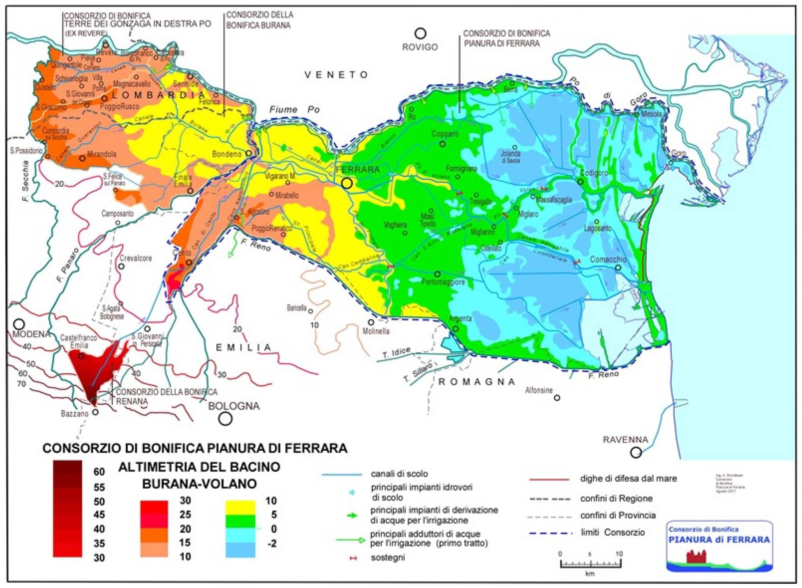
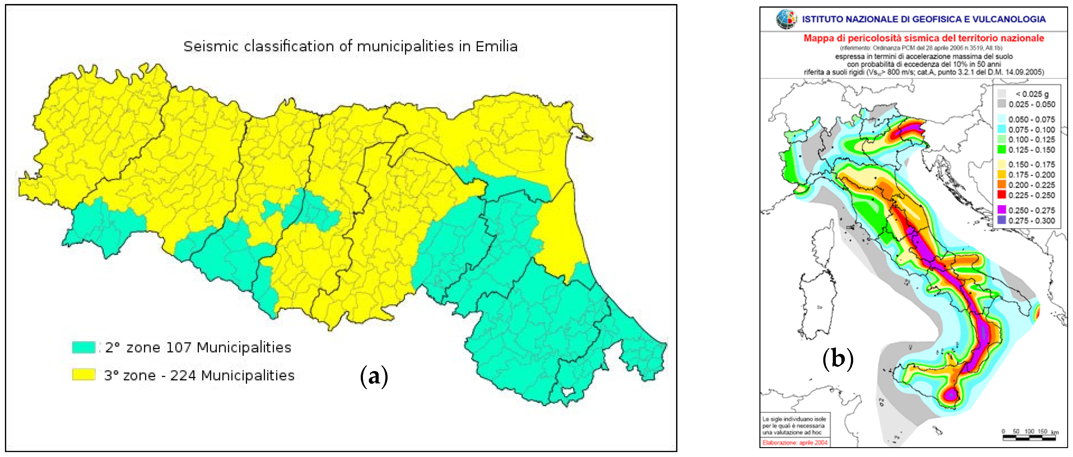
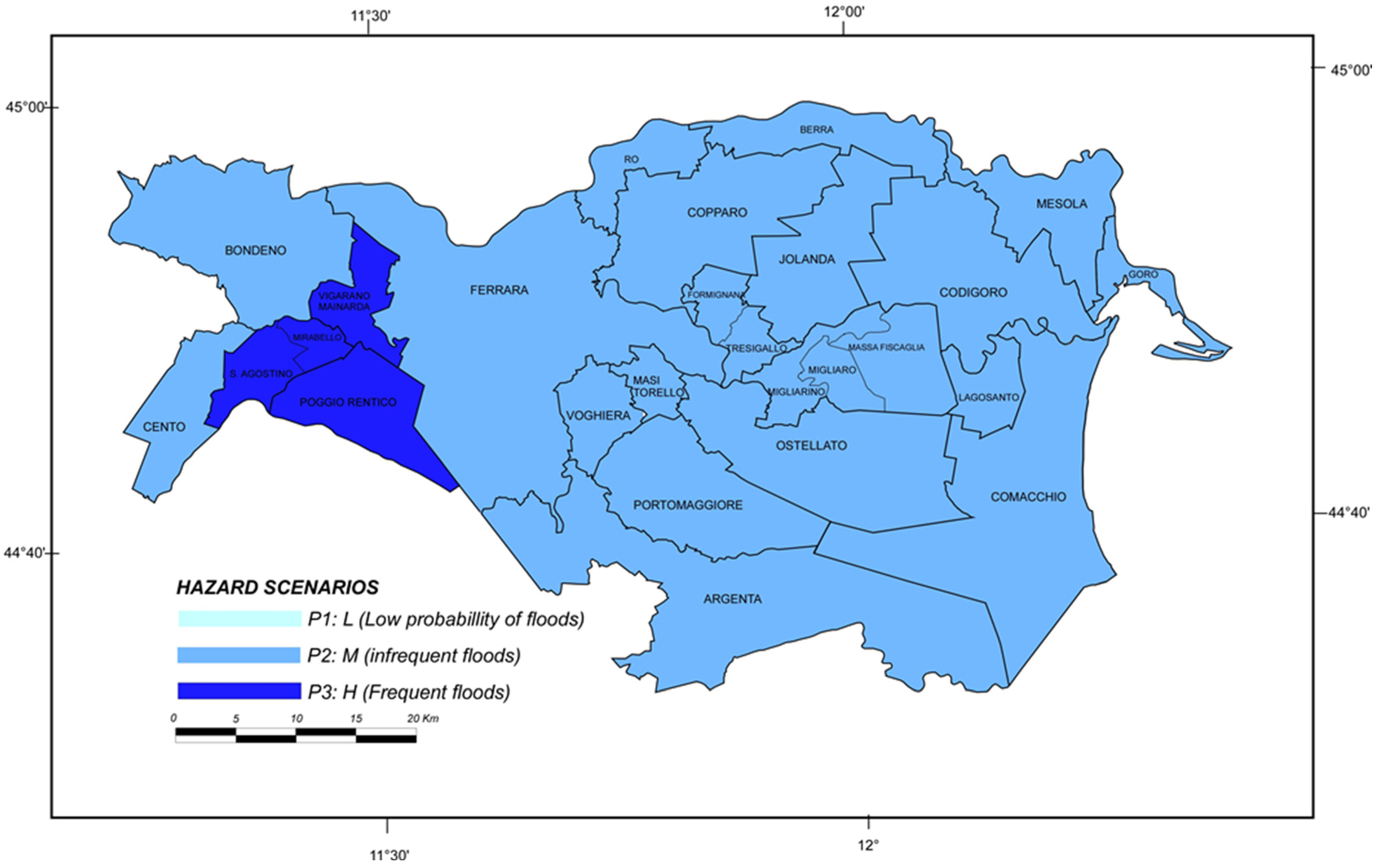
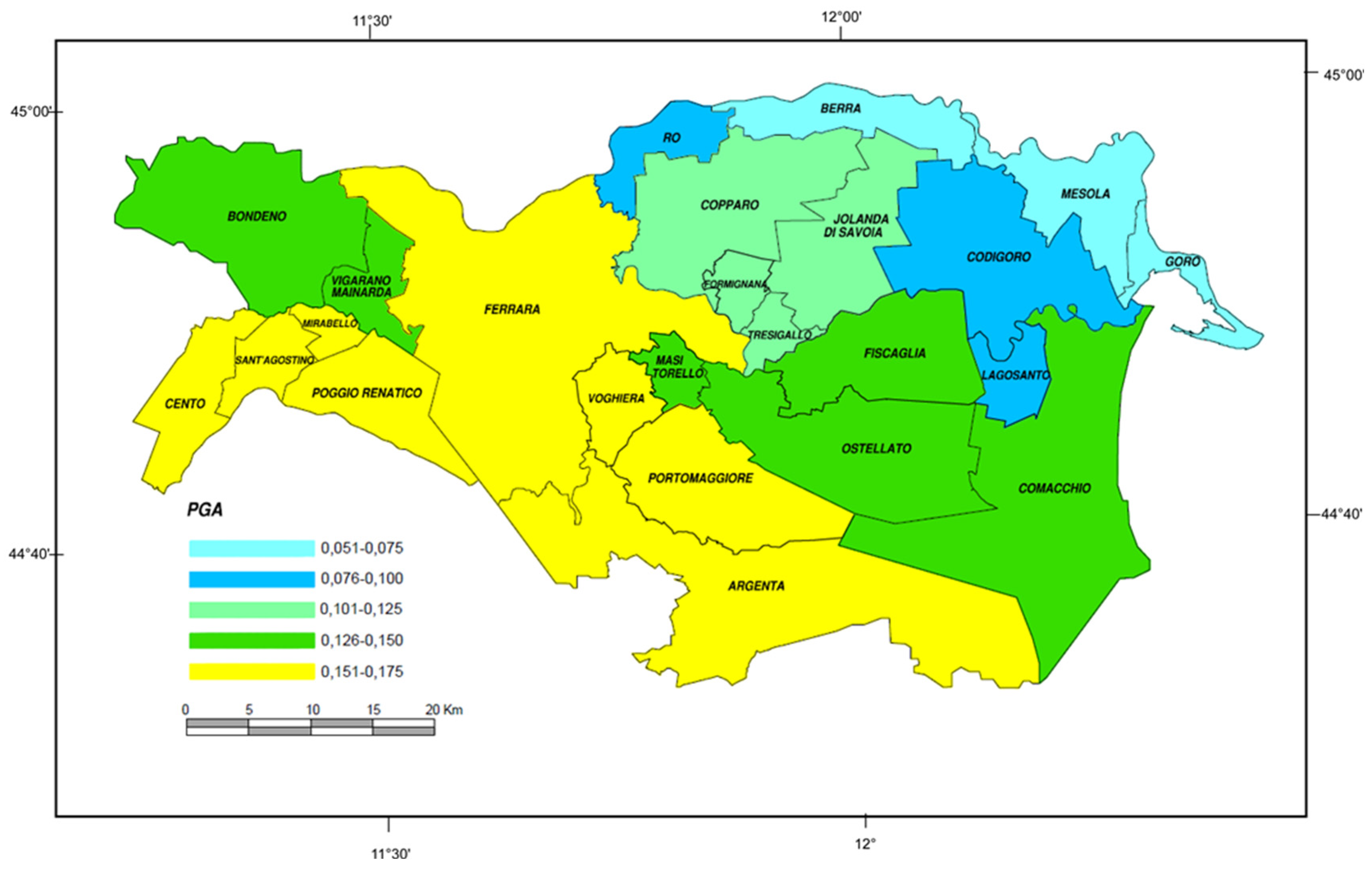
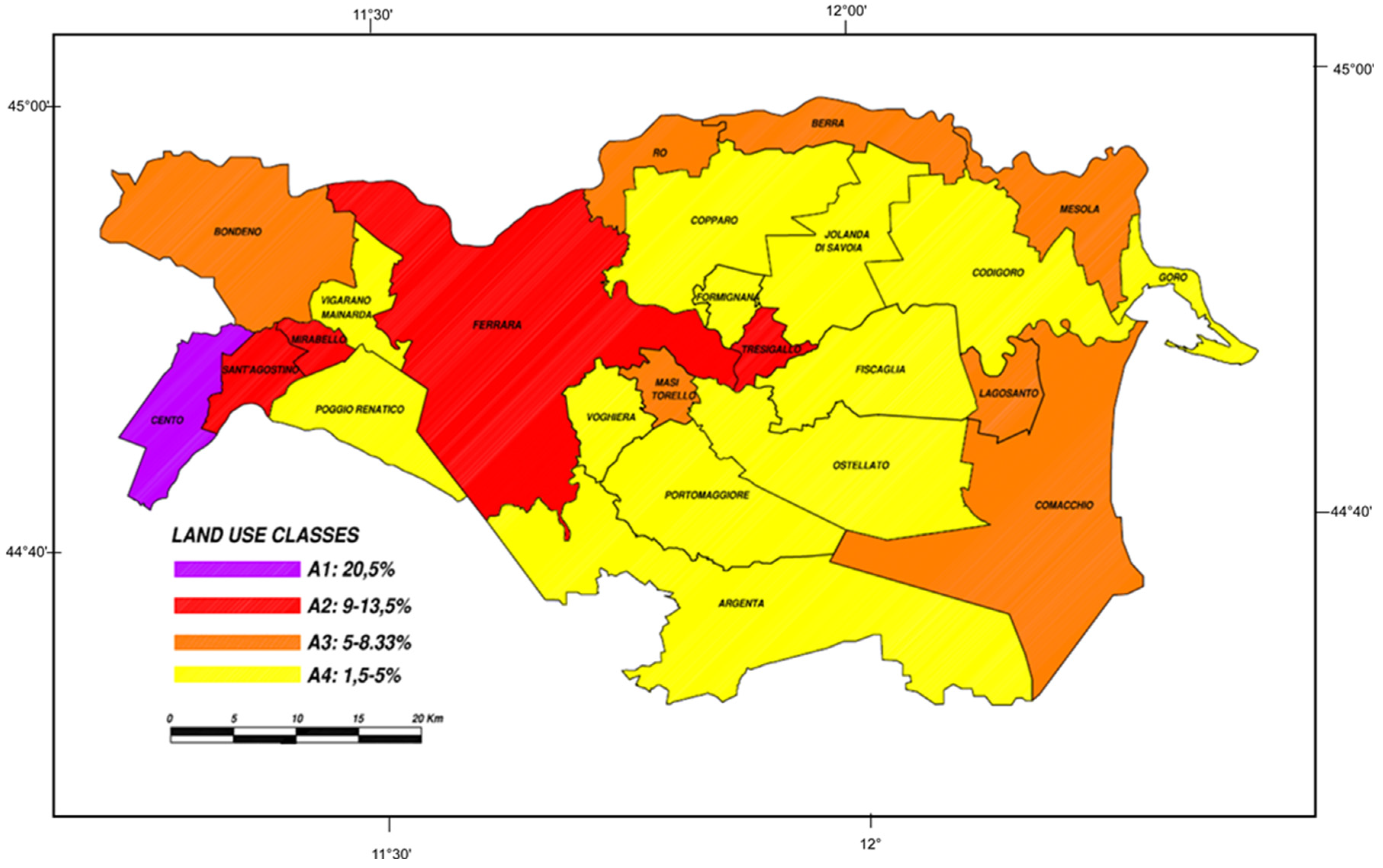
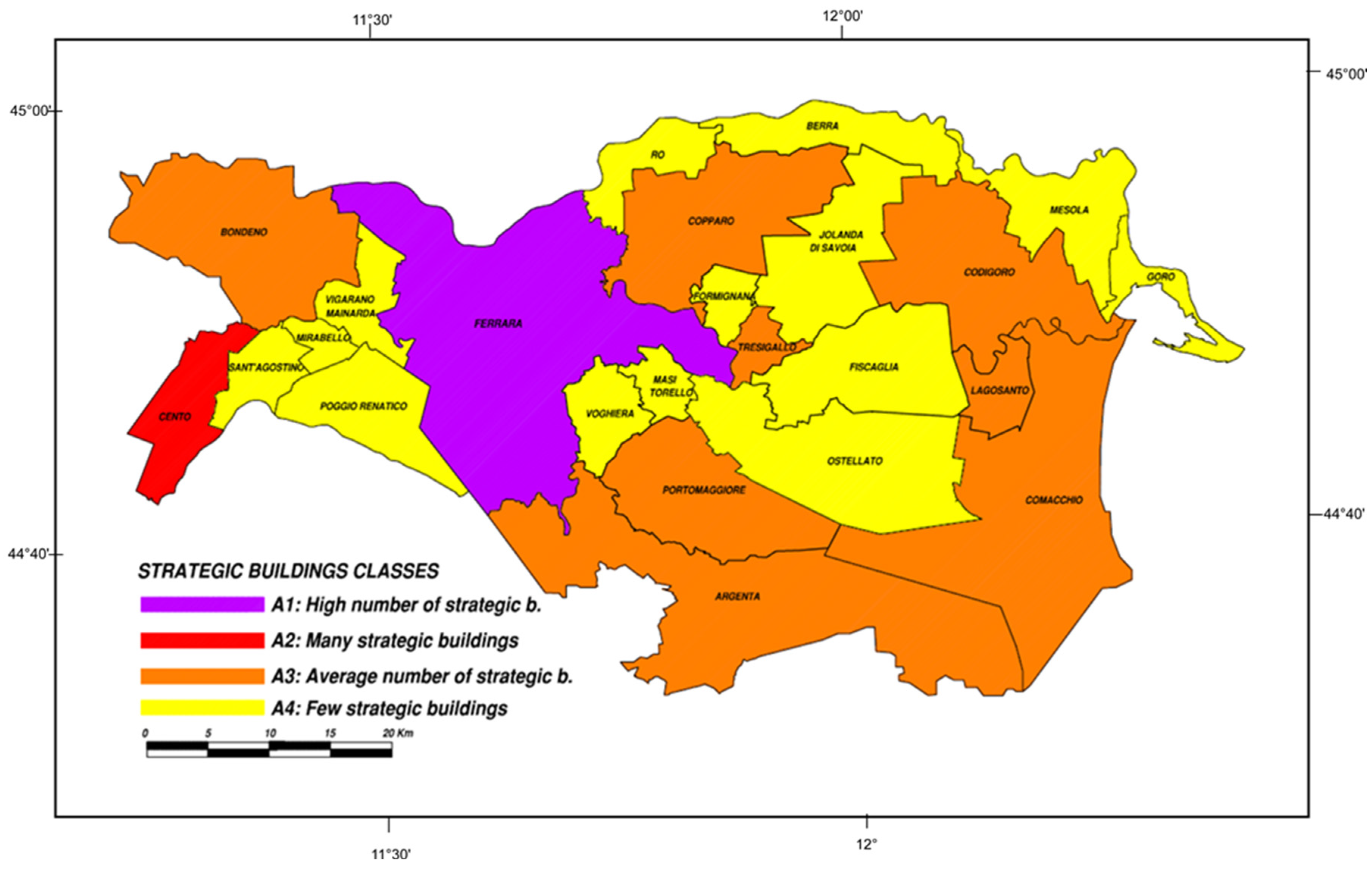
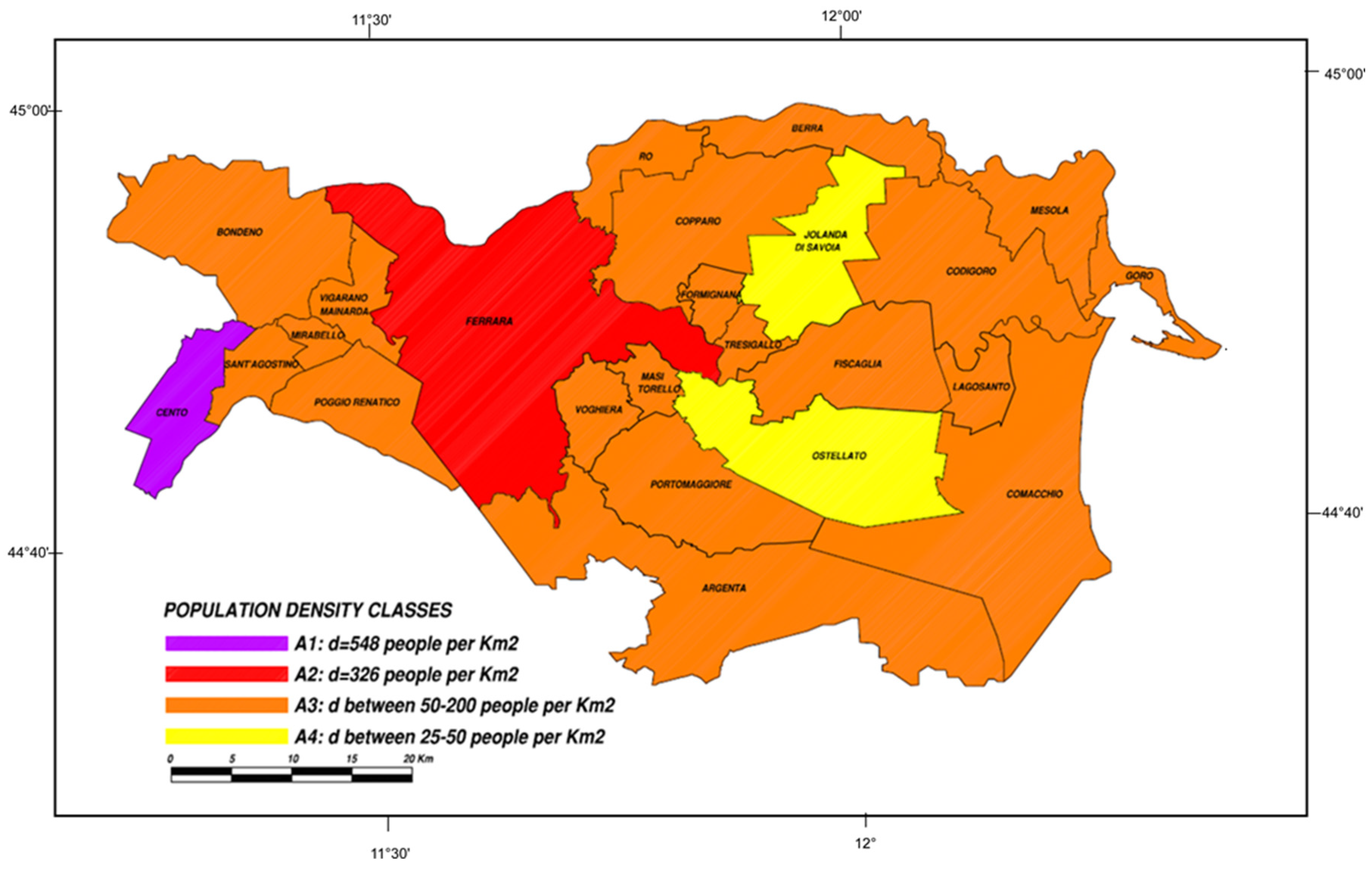
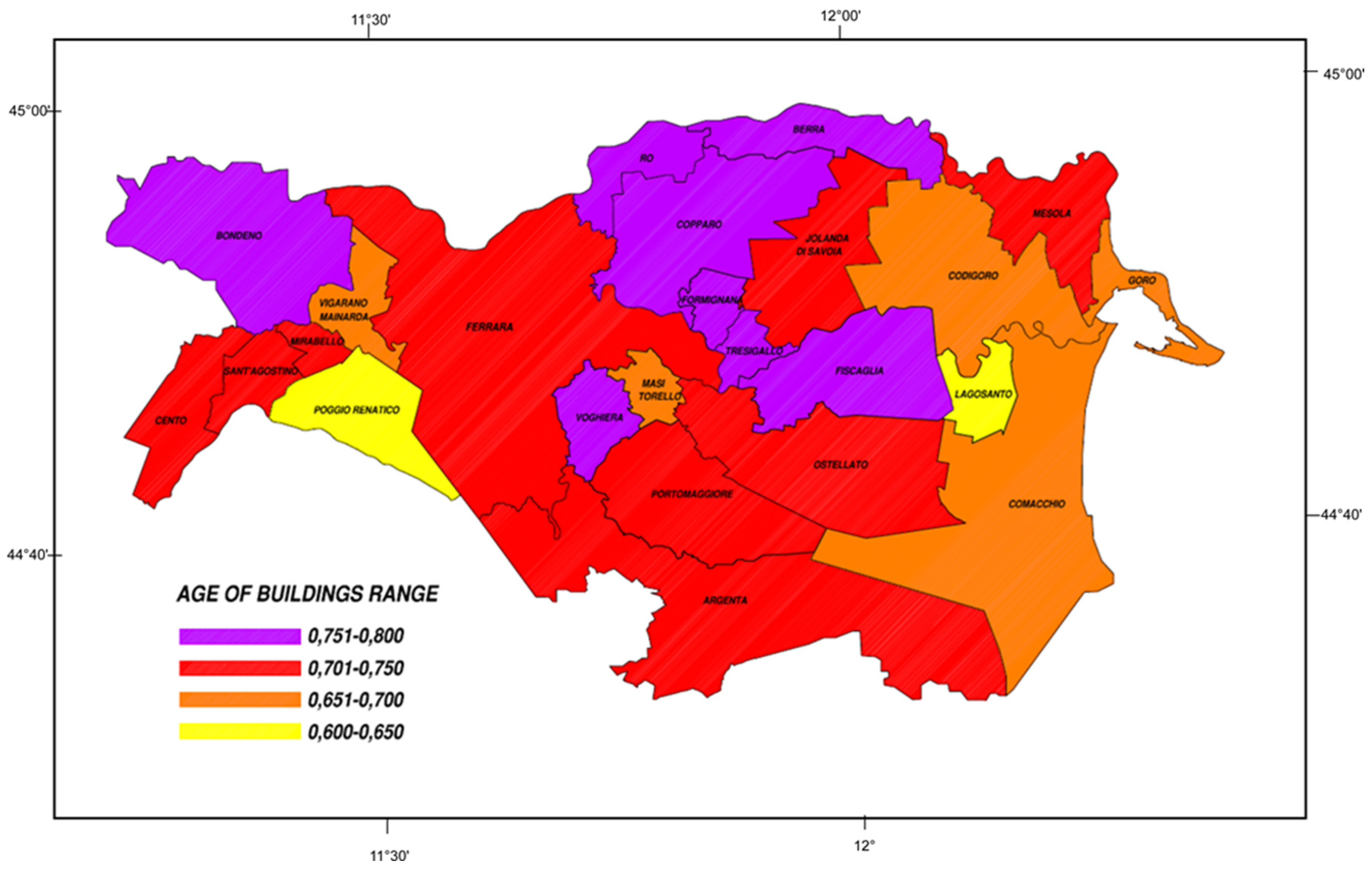
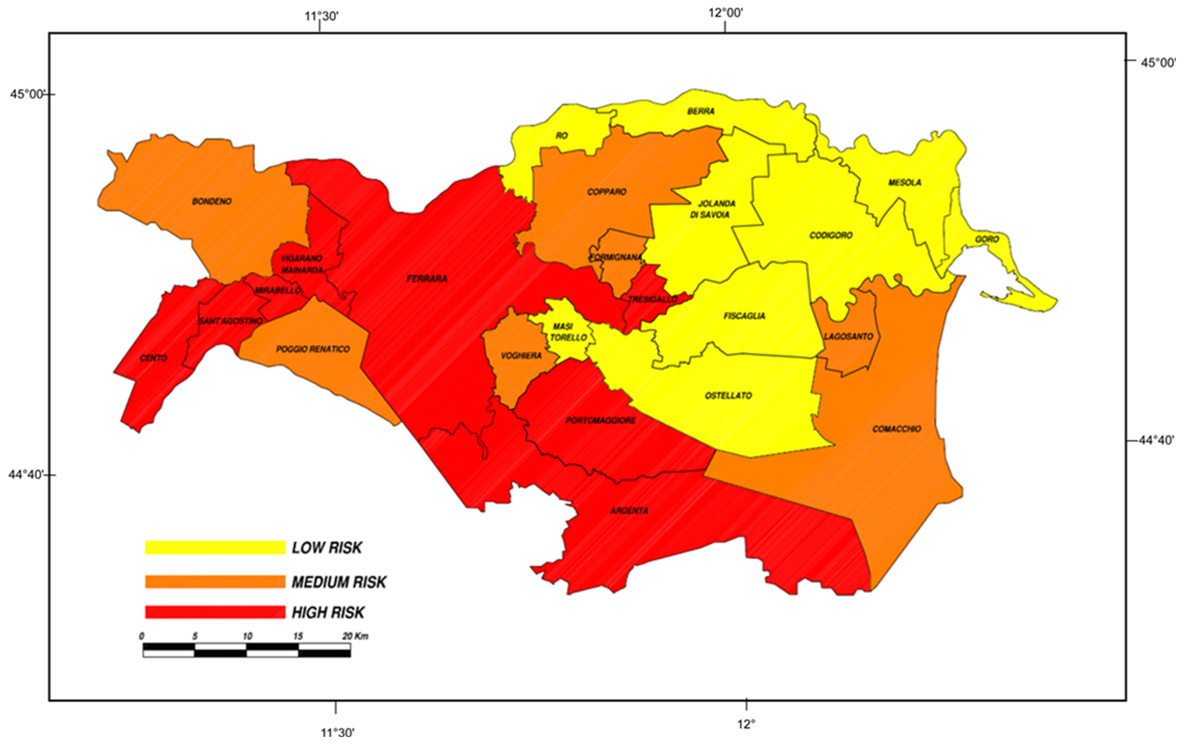
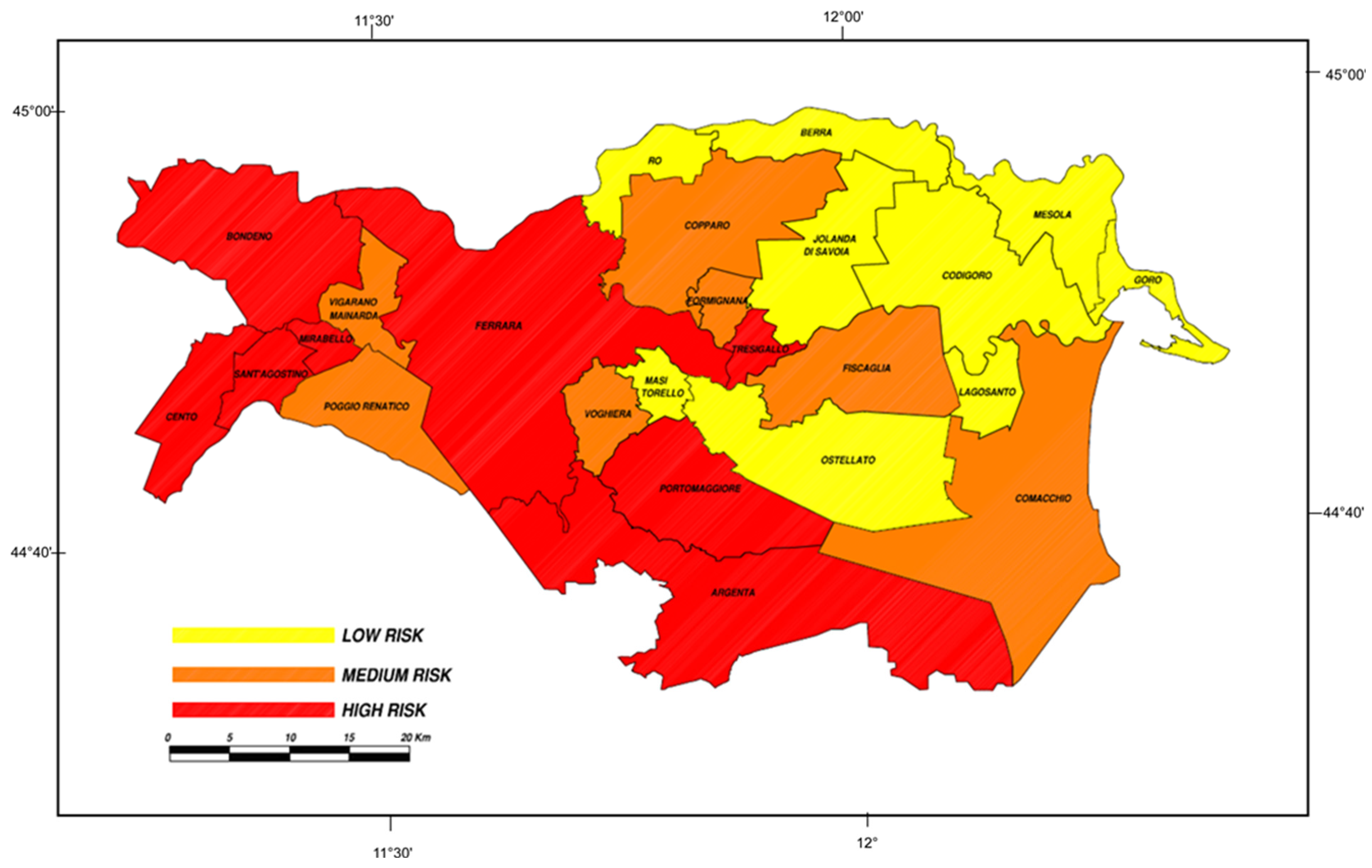
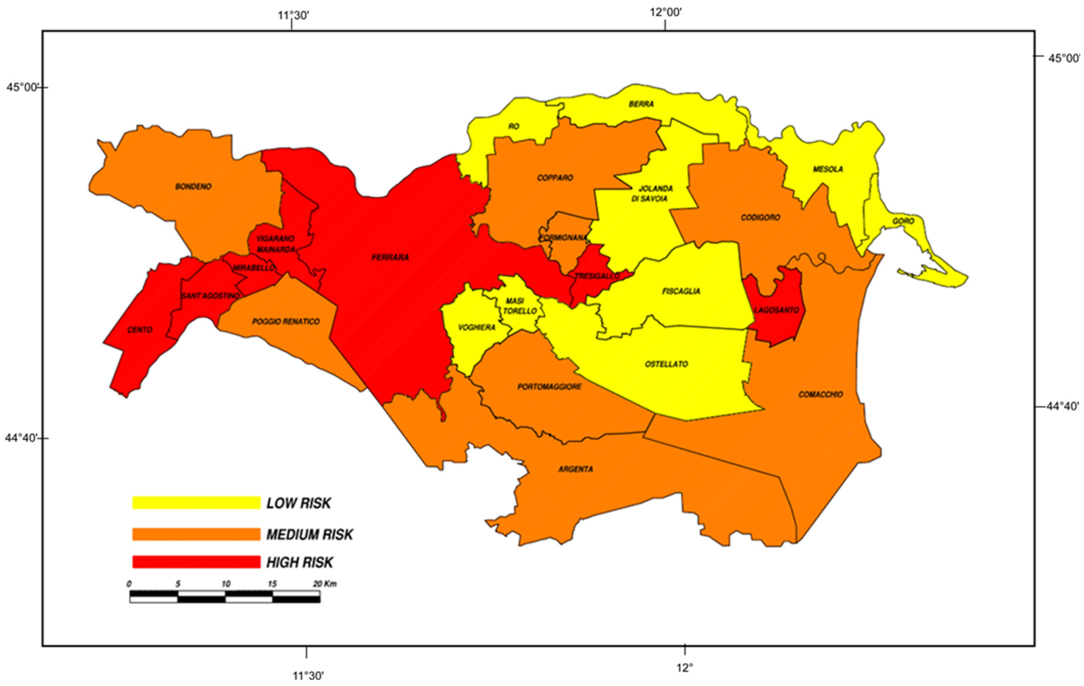
2.1. Geographical Context and Single Risk Description

To introduce the concept of multi-risk assessment, it is first necessary to discuss the concept of single risk. Risk is basically defined as the product of three parameters: Hazard, vulnerability, and exposure [9]. A hazard represents the probability that an adverse event will occur in a specific area and in a specific time interval. Vulnerability, on the other hand, is an intrinsic characteristic of a system; it represents its propensity to suffer a certain level of damage following the occurrence of a hazard event. Finally, exposure indicates the presence of people, critical infrastructures, natural and cultural heritage, and much more still in hazard zones that are thereby subject to potential losses [4].
The concept of multi-risk follows as the overall risk from a multi-hazard and multi-vulnerability perspective. The term multi-hazard indicates several hazards affecting the same exposed elements (with or without space–time coincidence) or the occurrence of a hazard event that triggers another one giving rise to a domino or cascade effect. Furthermore, the term multi-vulnerability indicates those circumstances where several elements are sensitive to different possible vulnerabilities towards the various hazards affecting them or vulnerabilities that vary over time [10,11].
The territory of the province of Ferrara is located at the north-eastern extremity of the Padana Plain, a flat land area in the north part of Italy crossed by the Po River and bathed by the Adriatic Sea on the east side. It is characterized by minimum land slopes and its altimetry is mainly under the mean sea level, as almost half of its area is below the mean sea level, as shown in Figure 1. Moreover, the eastern part of the territory is affected by subsidence phenomena as well. These ground-level modifications, caused mainly by anthropogenic actions as well as by geological and neotectonic factors [31,32], produced a subsidence rate of up to −2.5 mm/year [31]. The main watercourses that flow through the Ferrara province are the Po River, which marks the northern border of the Reno River, and the Idice and Sillaro streams, which are not tributaries of the Po River, and cross the province in their last stretch. Furthermore, numerous artificial canals flow through the Ferrara Province, including the Cavo Napoleonico, which connects the Po and Reno rivers, and the Idrovia Ferrarese.
The province of Ferrara includes 23 municipalities. Attention is hereafter restricted to the two main risks of the area under study, namely flood and seismic risks. Site effects associated with inherent geological morphology and instability issues such as liquefaction were not considered, for simplicity. Desertification is another risk that has been emerging in recent years in the Po delta plain [10]. However, it has not been considered in the present contribution. Hereafter, flood risk refers to the risk that depends on the probability of occurrence of a flood, evaluated concerning the different typologies of watercourses that flow through the territory. The flood risk for the selected region was quantified by the Land Reclamation Authority of the province of Ferrara (Consorzio di Bonifica Pianura di Ferrara), and accounts for flood hazard, exposure, and vulnerability parameters.
Seismic risk depends on the peak ground acceleration (PGA) as well as on the vulnerability of the built environment and the exposure of people and economic activities. We exploited the map of seismic hazard provided by the Italian Institute of Volcanology and Geophysics (INGV), and the seismic classification of municipalities in Emilia (free source https://ambiente.regione.emilia-romagna.it/en/geologia/seismic-risk/seismic-classification, accessed on 26 January 2022), shown in Figure 2a. In Figure 2b, Italy is divided into different areas according to peak ground acceleration values [33] (free source http://zonesismiche.mi.ingv.it/, accessed on 26 January 2022).
Finally, we used the database made available by the Italian National Institute of Statistics (Istat). This database was used in 2018 by the Italian Superior Institute for Environmental Protection and Research (ISPRA) to produce seismic, hydrogeological, volcanic, and social vulnerability hazard maps for the entire Italian peninsula. The reader is referred to the pertinent report by Trigila et al. [34] to obtain a detailed description of ISPRA’s methodology for the processing of the data.

2.2. The PROMETHEE Method

The proposed multi-hazard risk analysis procedure for the region under study is based on PROMETHEE [26,27,28,29], a Multiple-Criteria Decision Analysis method. It belongs to the class of aggregation methods based on outranking relationships. It is known for its simplicity and the ability to analyze information from multiple sources. PROMETHEE allows one to jointly compare data originally expressed in different units and scales. A flux diagram explaining the various steps of the PROMETHEE-based analysis can be found in reference [29].
PROMETHEE deals with maximization or minimization problems with k different criteria of the kind
max ( o r min ) { g 1 ( a ) , g 2 ( a ) , , g k ( a ) | a A } ,
where A is a finite set of possible alternatives and function g j ( a ) represents the performance of the j-th criterion. Let us consider two alternatives, ( a , b ) A . We have the following cases:
{ j : g j ( a ) g j ( b ) k : g k ( a ) > g k ( b ) a P b , j : g j ( a ) = g j ( b ) a I b , { s : g s ( a ) > g s ( b ) r : g r ( a ) < g r ( b ) a R b ,
where P, I, and R denote preference (P), indifference (I), or incompatibility relations (R) of one alternative over the other, respectively.
By comparing all the alternatives for each criterion, a hierarchy of alternatives belonging to the starting space A will be obtained. When comparing two actions, ( a , b ) A . the result of this comparison is expressed in terms of the preference function :   A × A ( 0 , 1 ) that represents the intensity of the preference of alternative a towards alternative b. Therefore, ( a , b ) = 0 indicates no preference of a over b (or indifference), ( a , b ) 0 indicates a weak preference of a over b, ( a , b ) 1 indicates a strong preference of a over b, and ( a , b ) = 1 indicates a strict preference of a over b. In practice, the preference function will often be a function of the difference between the evaluations of the two alternatives considered:
( a , b ) = P ( g ( a ) g ( b ) ) = P ( d ) ,
where P is a non-decreasing function, equal to zero for negative values of d. PROMETHEE offers six types of preference functions (see Table 1).
Therefore, a preference index is defined as follows:
{ π ( a , b ) = j = 1 k P j ( a , b ) w j π ( b , a ) = j = 1 k P j ( b , a ) w j ,
where π ( a , b ) expresses the degree to which a is preferred to b over all criteria and vice versa, and w j is the weight of each criterion and expresses a measure of the importance of the relative criterion.
For all the criteria, a classification is available for the various alternatives necessary to define the so-called outranking flows, which are the fundamental units for the PROMETHEE methodology. Each alternative a faces ( n 1 ) other alternatives that belong to the generic space A. The two following outranking flows are defined:
{ Θ + ( a ) = 1 n 1 x A π ( a , x ) Θ ( a ) = 1 n 1 x A π ( x , a ) ,
where x represents the deviation of the specific preference function with respect to the same function of preference for the other alternatives. Θ + ( a ) expresses how alternative a outranks all the others, otherwise Θ ( a ) expresses how alternative a is outranked by all the others. The higher Θ + ( a ) (lower Θ ( a ) ) is, the more likely alternative a is strongest; otherwise, alternative a, compared to the others, is weakest when Θ + ( a ) assumes small values. Once these two flows have been defined, it becomes very simple to make comparisons between alternatives and subsequently establish their order.
PROMETHEE offers several ways to view the results; the main ones are illustrated below:
  • PROMETHEE I Partial Ranking: This is a partial ranking of the alternatives, based on positive and negative flows, and includes preferences, indifference, and incomparability. This scheme allows, therefore, to compare, where possible, the alternatives and establish their partial order of preference through the indices and the related outranking flows.
  • PROMETHEE II Complete Ranking: This is useful when the decision maker needs a complete hierarchy among the alternatives of the problem. In this case, the alternatives will be compared in relation to their net flow Θ ( a ) = Θ ( a ) + Θ ( a ) . PROMETHEE II allows a complete classification of the alternatives; however, it is less realistic and poor in information as it eliminates any possible factor of incomparability between the different alternatives.
  • PROMETHEE Table: This displays the Θ , Θ + , and Θ scores. The actions are ranked according to the PROMETHEE II complete ranking.
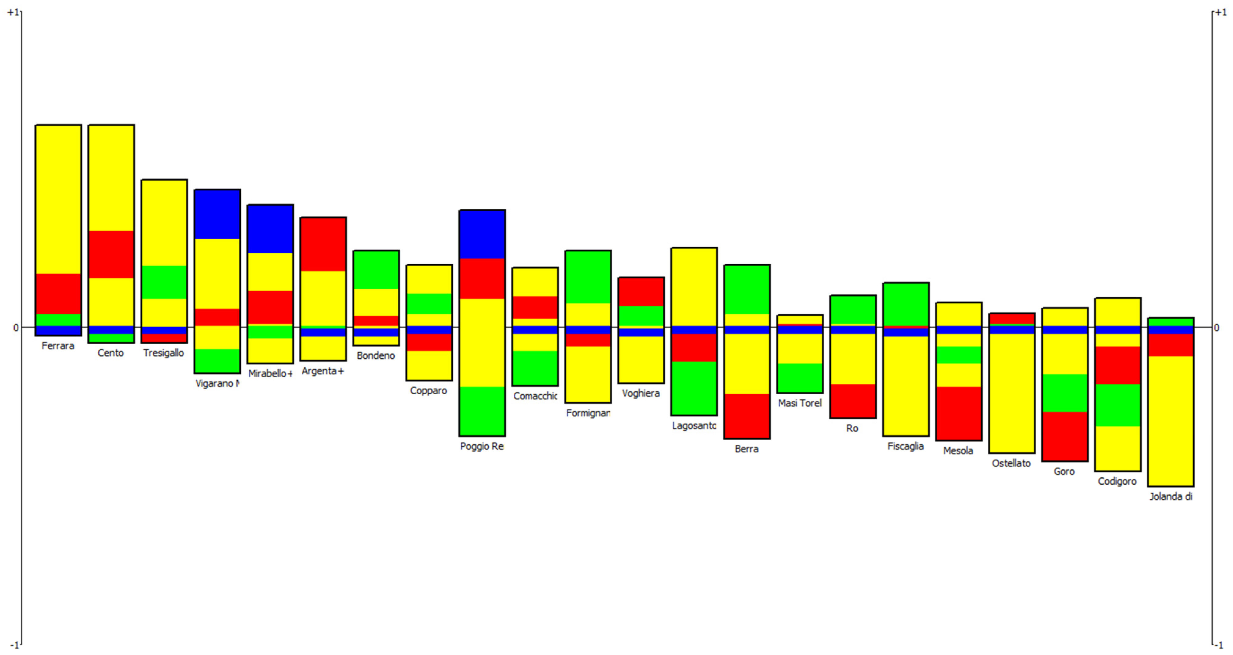
  • PROMETHEE Rainbow: This is a diagram that allows one to highlight, for each alternative, the criteria that positively or negatively affect the final result.
  • Profile of alternatives: This is a diagram that shows, for each alternative, the net flow Θ of each criterion.

2.3. Data Collection and Processing

Both flood and seismic risks have been included in PROMETHEE as criteria according to their components (hazard, exposure, and vulnerability), while the municipalities, i.e., the object on which to evaluate the criteria, are the alternatives. Risk parameters for each municipality are made available by the National Institute of Vulcanology and Geophysics (INGV), the Italian National Institute of Statistics (Istat), and the Land Reclamation Authorities of the Province of Ferrara. Accordingly, we have drawn from the aforementioned databases a simplified map of the flood risk. In particular, Figure 3 displays the flood hazard for the Province of Ferrara in terms of the probability of floods. In this map, the classification is based on Italian Government Decree n. 49/2010 [35]. Accordingly, frequent floods are defined as those having a high probability of occurrence, with a return period of 20 ≤ T ≤ 50 years (P3); infrequent floods have an average probability of occurrence with a return period of 100 ≤ T ≤ 200 years (P2); finally, low-probability floods have a return period of 200 < T ≤ 500 years (P1).
Figure 4 provides a map of the seismic hazard for the province of Ferrara in terms of peak ground acceleration (PGA). The PGA-intervals are indicated in the legend.
As for exposure-related criteria, for each municipality, we adopted three parameters: Land use percentage, the number of strategic buildings, and population density. All of them were drawn from the Istat database. The strategic buildings were defined based on the presence and number of halls, police stations, fire brigade buildings, schools, universities, water lifting plants, hospitals, and civil protection centers. This information was obtained from the website of the province of Ferrara (http://www.provincia.fe.it/, 1 October 2021), as per educational and public institutions and centers, and from the website of the Consorzio di Bonifica Pianura di Ferrara as per water lifting plants (https://www.bonificaferrara.it/, 1 October 2021).
Specifically, four classes of land use percentages were obtained based on the ratio between the urbanized area divided by the total area. In synthesis, we collected the municipalities into four land use classes (Figure 5), four classes in terms of the number of strategic buildings (Figure 6), and four classes of population density (Figure 7).
As for the vulnerability criteria, we adopted a single non-dimensionalized parameter, which accounts for the average age of buildings. Knowing the age of construction and the corresponding number of buildings, we computed the following vulnerability index:
I v = A   α 1 + B   α 2 + C   α 3 + D   α 4   A + B + C + D   ,
where A ,   B ,   C   e   D represent the number of buildings built between the end of 1800 and 1945; the number of buildings built between 1946 and 1980; the number of buildings built between 1981 and 2000, and finally, the number of buildings built from 2001 up to now. α 1 ,     α 2 ,   α 3   e   α 4 are coefficients equal to 1, 0.75, 0.5, and 0.25, respectively. The vulnerability index Iv results in being mainly related to the age of buildings, and its map is shown in Figure 8.

2.4. Normalization and Weight Assignment

All the data have been collected in an evaluation matrix, whose rows correspond to each alternative (i.e., each municipality), while each column corresponds to each selected criterion. In other words, the i,j-th element of the evaluation matrix expresses the value of the i-th alternative relating to the attribute of the j-th criterion and describes the performance of each alternative regarding each criterion.
It should be noted that criteria are represented through different scales and units. This precludes mutual comparisons. Thus, it is necessary to further homogenize the data contained in the evaluation matrix and proceed with comparisons through normalization. Through the preference function, the performance of the alternatives is transformed into a dimensionless value, ranging from o to 1. As a first attempt, we adopted the Type 1 preference function described in Table 1, which does not require the definition of any threshold. Subsequently, the linear preference function was also used.
Finally, we attributed weights to each criterion. Through this step, decision makers can make their preferences explicit, since it is not ensured that all the criteria take on the same importance. We first decided to attribute the same weight to each criterion. Then, a sensitivity analysis was performed with varying weights.
The risk maps shown in the following sections indicate three classes of risk levels, namely low, medium, high. It is emphasized that this classification must be intended as a pure ranking in terms of the relative urgence of investments. It does not at all intend to indicate the level of safety in absolute terms of the various municipalities. This classification answers the question as to whether the method can provide the priority level associated with a certain municipality and help to decide how to distribute investments over various municipalities.

2.5. Sensitivity Analysis

To verify the reliability of the results obtained, a sensitivity analysis was carried out. During this sensitivity analysis, we retraced the procedure by which the results were obtained and identified the steps most affected by uncertainties and subjectivity, considering their influence on the final ranking. Specifically, the choice of the preference function and the choice of weights appeared to be the most subjective. As for the choice of the preference function, a previous study [26] recommends assuming a linear preference function endowed with the definition of p, q thresholds. Two approaches are adopted for the determination of p and q: The so-called zero-max method, which imposes that the indifference threshold q is assigned the value of zero while the preference threshold p is set to be equal to the maximum difference between the evaluations of the criteria.
The mean-std method requires the calculation of the average value and the standard deviation of a set of differences between the evaluations of the criteria. In the mean-std method, the indifference threshold is assigned the value of the difference between the average value and standard deviation, while the sum between the average value and standard deviation is assigned to the preference threshold. Following [26,27,28], we adopted the preference function of the linear type for the quantitative criteria, that is flood hazard, land use, the age of buildings, and population density. However, the algorithm was also run by choosing the usual preference function, which is the simplest possible one. The thresholds were computed as shown in Table 2. As for the sensitivity on the weights, the four scenarios described in Table 3 have been considered.

3. Results

In the following Section, we describe the outcomes of the multiple-criteria analysis for the usual and linear preference function as well as the results of the sensitivity analysis performed for varying weight changes.

3.1. Usual Preference Function

When the usual preference function is used, the algorithm assumes equal weights. We recall that, here, thresholds p and q are not required. Basically, what is provided to the analyst is an order of priority where the municipalities in the province of Ferrara are ordered from the most sensitive to combined flood and seismic risk to the one that is least affected. Table 4 shows the final ranking of the alternatives.
This is not the only way to visualize the results: The PROMETHEE rainbow plot, shown in Figure 9, allows one to highlight, for each alternative, the criteria that positively or negatively affect the results. In Figure 9, the colors are representative of the criterion: Yellow indicates the criteria relating to exposure, red is used for seismic hazard, green for vulnerability, and blue for flood hazard. For example, for the municipality of Ferrara (first in the ranking), it can be observed that the criterion that has a negative effect is the one relating to the flood hazard, whereas the other criteria have a positive effect on the Ferrara municipality. On the contrary, in the municipality of Jolanda di Savoia (last in the ranking), the only criterion that has a positive influence is the one relating to vulnerability, while all the others have a negative influence.
Based on the ranking provided by PROMETHEE, it is possible to create a risk map of the municipalities of the province of Ferrara that highlights high-priority areas as those with a high level of combined flood and seismic risk, medium priority areas as the areas characterized by a medium combined-risk level, and, finally, low combined-risk areas.
This map is shown in Figure 10. It can be seen that the three risk levels are identified by three different colors: Red is used for high risk, orange for medium risk, and yellow for low risk.

3.2. Linear Preference Function

The ranking of alternatives for the linear preference function and zero-max method is shown in Table 5, while the corresponding multi-risk map is shown in Figure 11. These maps were obtained by associating the quantitative criteria, i.e., flood hazard, land use, age of buildings, and population density, with a linear preference function, while thresholds q and p were determined with the zero-max method.
For a linear preference function of the aforementioned quantitative criteria, and thresholds q and p determined by the mean-std method, we obtained the results shown in Table 6 and Figure 12.
By comparing the results obtained from the usual and the linear preference functions, it can be understood that changes of the preference function do not reflect large changes of the final risk maps. The only difference is that the risk levels of the municipality of Vigarano Mainarda swap with Bondeno, and Fiscaglia swaps with Lagosanto.
By comparing the maps in Figure 11 and Figure 12, obtained with the thresholds chosen with the zero-max and mean-std methods, respectively, we observe that the risk levels of Lagosanto, Vigarano Mainarda, and Codigoro increase. Particularly, we observe that the choice of the preference function affects the final ranking of the alternatives especially when the thresholds are chosen according to the mean-std method.
Regardless of the preference function chosen, the maps obtained present a similar risk trend, i.e., the territory is divided into two parts: The municipalities of the western part of the territory of the province of Ferrara, plus Ferrara and Tresigallo, are characterized by a medium–high risk level; the upper-eastern part of the province is characterized by a medium–low risk level.

3.3. Sensitivity Analysis on the Choice of Weights

As introduced in Section 2, the sensitivity analysis on the weights was performed by first increasing the weight of each individual criterion at a time, and then assuming the simultaneous increase in the weights of the three “exposure”-related criteria, namely land use, population density, and strategic buildings. Specifically, the weights were changed according to Scenarios 0, 1, 2, and 3 described in Table 3.
For the sake of brevity, we present hereafter the results obtained by assuming the usual preference function. For the reader’s convenience, the results are reported as maps, as in the previous sections.
In the first part of the analysis, the criteria are changed according to the following order: Flood hazard, PGA, land use, strategic buildings, age of buildings, and population density. Hereafter, we omit the maps obtained for the changes of the weights relating to the criteria of strategic buildings and age of buildings, for brevity. Figure 13 and Figure 14 illustrate the various risk maps obtained by increasing the weights.
With Scenario 1 based on the variation of the flood hazard weight, the ranking of the municipalities remains almost unchanged, as the multi-risk map is identical to that of Scenario 0. On the other hand, the maps change when Scenarios 2 and 3 are adopted, as shown in Figure 13a. More marked differences can be observed when the weight of the PGA (Figure 13b,c) is changed. By increasing the weight of the land-use criterion, an increase in Scenario 1 does not reflect evident changes in the multi-risk map (Figure 13d). On the other hand, changes in Scenarios 2 and 3 affect the multi-risk map. Looking back at the strategic building criterion, we observe differences in the risk map when the first change of Scenario 1 is applied, compared to Scenario 0 (Figure 13e), and more so with the last two increases of Scenario 2 (Figure 13f). For the criterion of population density, the first increase in the weight according to Scenario 1 does not affect the map (see Figure 14a), while the subsequent increases in the weight bring about noticeable modifications. In particular, the multi-risk map reported in Figure 14b assigns a comparatively low level of attention to the Argenta municipality, which, however, is associated with a medium seismicity level according to the territorial classification of Figure 2a. Depending on the stakeholders’ expectations, this might suggest that weights should not be varied to the extent of downgrading the seismic risk level of certain municipalities classified at medium to high seismic risk.
Lastly, results of the sensitivity on the weight choice for the criteria related to exposure are presented in Table 7. Proceeding as illustrated in Section 2, the first increase in the weight does not alter the risk map, which remains the same as in Scenario 0, whereas with the changes of Scenario 2, greater variations can be observed.
Therefore, concluding the sensitivity analysis of weights, it can be inferred that, in general, the results are sensitive to the increase in the weights of the criteria, determining a risk map that varies from case to case, causing the risk of some municipalities to decrease while that of others increased. However, these variations do not upset the overall trend, which highlights a territory divided into two parts, that of the municipalities of the western part of the territory of the province of Ferrara characterized by a medium–high risk level, and the municipalities of the north-eastern area characterized by a medium–low risk level.

3.4. Remarks on the Limitations of the Analysis

The proposed methodology requires the definition of several parameters, criteria, and weights, whose choice resulted in being strongly dependent on the expectations of stakeholders and end-users. Thus, the obtained results should be seen as a first attempt towards the proposal of an MCDA methodology that does not require great mathematical expertise, is flexible, and can be easily adapted to many situations. Nevertheless, further efforts are necessary in order for the tool to be readily exploited by public authorities and decision makers. Furthermore, it is worth highlighting other limitations inherent in the present analysis.
The first type of limitation is mainly related to the availability of data. Indeed, the choice of the criteria was based on the availability of the relevant information, which led, for some criteria, to a purely qualitative evaluation. Greater availability, accuracy, and ease of retrieval of the data would lead to the creation of a more complete and more precise analysis, and it could also contribute to the development of operational tools and software.
Secondly, this analysis neglected cascade effects, an aspect that deserves further investigation in the future [11].
Thirdly, the present contribution does not consider the impact of modeling assumptions on the seismic risk assessment. At the relevant scale of observations of the present analysis, specific structural aspects connected to the vulnerability levels of the buildings cannot be easily considered. In this regard, we recall that specific structural aspects and modeling assumptions play, among others, a key role for seismic risk evaluation at both the building and the urban scale [36]. A recent study focusing on South America has shown the uncertainties and biases that the use of simplified models or heterogenous data may produce in the determination of seismic vulnerability [36]. For completeness, seismic risk evaluation is extensively discussed, for instance, in the aforementioned contributions [36,37,38,39] and the references cited therein.
Finally, we recall that the seismic classification shown in Figure 2 has been merely used as a technical-administrative reference for establishing the priority of actions and measures aimed at preventing and mitigating seismic risk. It must not be used to determine the local seismic action or for the structural design of buildings, which, instead, rely upon more detailed maps highlighting, for instance, the presence of site effects due to the inherent geological structure of the ground or instability effects such as liquefaction. Therefore, the present analysis should be purposefully extended in order to consider the aforementioned local effects [40].

4. Conclusions

For the present case study, the application of the Multiple-Criteria Decision Analysis (MCDA) methodology through the PROMETHEE algorithm has proved an innovative and promising operational tool. Its potential derives from the ability to both analyze information from various sources and jointly systematize data expressed in different units and scales. The application of this methodology has made it possible to rank the various municipalities in terms of the relative proneness to joint flood and seismic hazards. We recall that the objective of the methodology is not to quantify the safety level in absolute terms of the various municipalities. Its scope is, indeed, to provide useful information for decision makers and public authorities to define future intervention priorities. We further emphasize that, in the authors‘opinion, the present study is original as it applies the PROMETHEE algorithm for the first time to a multi-risk assessment of seismic and flood hazards.
Depending on the territory to be studied, the relevant risks could be different, and therefore, different criteria must be used to express them. Nevertheless, the generalization to other multi-risk analyses and different case studies deserves further considerable efforts and thoughtful insights. Full validation of the present methodology is also of utmost importance and calls for new developments. However, the proposed methodology is flexible. This suggests that, with due precautions and adaptations, it is possible to apply it to different risk scenarios, such as scenarios including coastal floods and landslides, while keeping the same applicative scheme.
Finally, the obtained results have shown that the proposed methodology is an operational tool that, once further validated, can be used by end users, whether modelers or decision makers, to urgently allocate resources and increase the coping capacity of communities in the case of catastrophic events.

Author Contributions

Conceptualization, Ž.N., A.C., C.V. and E.B.; methodology, Ž.N., A.S. and A.C.; software, A.S.; validation, A.S., A.C. and C.V.; formal analysis A.S., A.C., Ž.N. and C.V.; resources E.B.; data curation, A.S.; writing—original draft preparation, A.S. and A.C.; writing—review and editing, A.C., C.V., Ž.N. and E.B.; visualization, A.S. and A.C.; supervision, E.B.; project administration, E.B.; funding acquisition, E.B. All authors have read and agreed to the published version of the manuscript.

Funding

This research was funded by the EUROPEAN UNION, Programme Interreg Italy-Croatia, Project “Preventing, managing and overcoming natural-hazards risks to mitigate economic and social impact”—PMO-GATE ID 10046122.

Institutional Review Board Statement

Not applicable.

Informed Consent Statement

Not applicable.

Data Availability Statement

Acknowledgments

The authors are very grateful to Consorzio di Bonifica Pianura di Ferrara for making the flood maps freely available, and, particularly, to Eng. Alessandro Bondesan for his kind support in georeferencing the maps.

Conflicts of Interest

The authors declare no conflict of interest.

References

  1. UN-ISDR. Sendai Framework for Disaster Risk Reduction 2015–2030. In Proceedings of the UN world Conference on Disaster Risk Reduction, Sendai, Japan, 14–18 March 2015; United Nations Office for Disaster Risk Reduction: Geneva, Switzerland. Available online: http://www.unisdr.org/files/43291_sendaiframeworkfordrren.pdf (accessed on 1 October 2021).
  2. Poljanšek, K.; Ferrer, M.M.; De Groeve, T.; Clark, I. Preface. In Science for Disaster Risk Management 2017: Knowing Better and Losing Less; Publications Office of the European Union: Luxembourg, 2017; ISBN 978-92-79-60678-6. [Google Scholar] [CrossRef]
  3. Topics Geo: Natural Catastrophes 2013: Analyses, Assessments, Positions, Münchener Rückversicherungs-Gesellschaft, Munich. 2014. Available online: https://www.munichre.com/content/dam/munichre/contentlounge/website-pieces/documents/302-08121_en.pdf/_jcr_content/renditions/original./302-08121_en.pdf (accessed on 26 January 2022).
  4. UN-ISDR. Terminology: Basic Terms of Disaster Risk Reduction. 2009. Available online: http://www.unisdr.org./we/inform/terminology (accessed on 1 October 2021).
  5. Urlainis, A.; Ornai, D.; Levy, R.; Vilnay, O.; Shohet, I.M. Loss and damage assessment in critical infrastructures due to extreme events. Saf. Sci. 2022, 147, 105587. [Google Scholar] [CrossRef]
  6. Kanamori, H.; Hauksson, E.; Heaton, T. Real-time seismology and earthquake hazard mitigation. Nature 1997, 390, 461–464. [Google Scholar] [CrossRef]
  7. Quesada-Román, A.; Villalobos-Chacón, A. Flash flood impacts of Hurricane Otto and hydrometeorological risk mapping in Costa Rica. Geogr. Tidsskr.-Dan. J. Geogr. 2020, 120, 142–155. [Google Scholar] [CrossRef]
  8. Quesada-Román, A.; Ballesteros-Cánovas, J.A.; Granados-Bolaños, S.; Birkel, C.; Stoffel, M. Improving regional flood risk assessment using flood frequency and dendrogeomorphic analyses in mountain catchments impacted by tropical cyclones. Geomorphology 2022, 396, 108000. [Google Scholar] [CrossRef]
  9. Kron, W. Reasons for the increase in natural catastrophes: The development of exposed areas. In Topics 2000: Natural Catastrophes, the Current Position; Munich Reinsurance Company: Munich, Germany, 1999; pp. 82–94. [Google Scholar]
  10. Barredo, J.I. Major flood disasters in Europe: 1950–2005. Nat. Hazards 2007, 42, 125–148. [Google Scholar] [CrossRef]
  11. Zuccaro, G.; De Gregorio, D.; Leone, M. Theoretical model for cascading effects analyses. Int. J. Disaster Risk Reduct. 2018, 30, 199–215. [Google Scholar] [CrossRef]
  12. Zschau, J. Where are we with multihazards, multirisks assessment capacities? In Science for Disaster Risk Management 2017: Knowing Better and Losing Less; Poljansek, K., Marin Ferrer, M., De Groeve, T., Eds.; Publications Office of the European Union: Luxembourg, 2017; ISBN 978-92-79-60678-6. [Google Scholar] [CrossRef]
  13. Fuchs, S.; Keiler, M.; Zischg, A. A spatiotemporal multi-hazard exposure assessment based on property data. Nat. Hazard. Earth Syst. Sci. 2015, 15, 2127–2142. [Google Scholar] [CrossRef] [Green Version]
  14. Komentova, N.; Scolobig, A.; Garcia-Aristizabal, A.; Monfort, D.; Fleming, K. Multi-risk approach and urban resilience. Int. J. Disast. Res. Built Environ. 2016, 7, 114–132. [Google Scholar] [CrossRef]
  15. Marzocchi, W.; Garcia-Aristizabal, A.; Gasparini, P.; Mastellone, M.L.; Di Ruocco, A. Basic principles of multi-risk assessment: A case study in Italy. Nat. Hazards 2012, 62, 551–573. [Google Scholar] [CrossRef]
  16. Kappes, M.S.; Keiler, M.; von Elverfeldt, K.; Glade, T. Challenges of analyzing multi-hazard risk: A review. Nat. Hazards 2012, 64, 1925–1958. [Google Scholar] [CrossRef] [Green Version]
  17. Bell, R.; Glade, T. Multi-hazard analysis in natural risk assessments. WIT Trans. Ecol. Environ. 2004, 77, 1–10. [Google Scholar]
  18. Schmidt, J.; Matcham, I.; Reese, S.; King, A.; Bell, R.; Henderson, R.; Smart, G.; Cousins, J.; Smith, W.; Heron, D. Quantitative multi-risk analysis for natural hazards: A framework for multi-risk modelling. Nat. Hazards 2011, 58, 1169–1192. [Google Scholar] [CrossRef]
  19. Neri, A.; Aspinall, W.P.; Cioni, R.; Bertagnini, A.; Baxter, P.J.; Zuccaro, G.; Andronico, D.; Barsotti, S.; Cole, P.D.; Esposti Ongaro, T.; et al. Developing an Event Tree for probabilistic hazard and risk assessment at Vesuvius. J. Volcanol. Geotherm. Res. 2008, 178, 397–415. [Google Scholar] [CrossRef]
  20. Barthel, F.; Neumayer, E. A trend analysis of normalized insured damage from natural disasters. Clim. Chang. 2012, 113, 215–237. [Google Scholar] [CrossRef] [Green Version]
  21. Skilodimou, H.D.; Bathrellos, G.D.; Chousianitis, K.; Youssef, A.M.; Pradhan, B. Multi-hazard assessment modeling via multi-criteria analysis and GIS: A case study. Environ. Earth Sci. 2019, 78, 47. [Google Scholar] [CrossRef]
  22. Brans, J.P.; Mareschal, B. Promethee Methods. In Multiple Criteria Decision Analysis: State of the Art Surveys; Figueira, J., Greco, S., Ehrogott, M., Eds.; Springer: Berlin/Heidelberg, Germany, 2005. [Google Scholar]
  23. Gallina, V.; Torresan, S.; Critto, A.; Sperotto, A.; Glade, T.; Marcomini, A. A review of multi-risk methodologies for natural hazards: Consequences and challenges for a climate change impact assessment. J. Environ. Manag. 2016, 168, 123–132. [Google Scholar] [CrossRef]
  24. Gallina, V.; Torresan, S.; Zabeo, A.; Critto, A.; Glade, T.; Marcomini, A. A Multi-Risk Methodology for the Assessment of Climate Change Impacts in Coastal Zones. Sustainability 2020, 12, 3697. [Google Scholar] [CrossRef]
  25. Peduzzi, P.; Dao, H.; Herold, C.; Mouton, F. Assessing global exposure and vulnerability towards natural hazards: The Disaster Risk Index. Nat. Hazards Earth Syst. Sci. 2009, 9, 1149–1159. [Google Scholar] [CrossRef]
  26. Brans, J.P.; Vincke, P.; Mareschal, B. How to select and how to rank projects: The PROMETHEE method. Eur. J. Oper. Res. 1986, 24, 228–238. [Google Scholar] [CrossRef]
  27. Mladineo, M.; Jajac, N.; Rogulj, K. A simplified approach to the PROMETHEE method for priority setting in management of mine action projects. Croat. Oper. Res. Rev. 2016, 7, 249–268. [Google Scholar] [CrossRef] [Green Version]
  28. Crnjac, M.; Aljinovic, A.; Gjeldum, N.; Mladineo, M. Two-stage product design selection by using PROMETHEE and Taguchi method: A case study. Adv. Prod. Eng. Manag. 2019, 14, 39–50. [Google Scholar] [CrossRef]
  29. Savic, M.; Nikolic, D.; Mihajlovic, I.; Zivkovic, Z.; Bojanov, B.; Djordjevic, P. Multi-Criteria Decision Support System for Optimal Blending Process in Zinc Production. Miner. Process. Extr. Metall. Rev. 2015, 36, 267–280. [Google Scholar] [CrossRef]
  30. Rocchi, A.; Chiozzi, A.; Nale, M.; Nikolic, Z.; Riguzzi, F.; Mantovan, L.; Gilli, A.; Benvenuti, E. A Machine Learning Framework for Multi-Hazard Risk Assessment at the Regional Scale in Earthquake and Flood-Prone Areas. Appl. Sci. 2022, 12, 583. [Google Scholar] [CrossRef]
  31. Carminati, E.; Martinelli, G. Subsidence rates in the Po Plain, northern Italy: The relative impact of natural and anthropogenic causation. Eng. Geol. 2002, 66, 241–255. [Google Scholar] [CrossRef]
  32. Salvati, L.; Mavrakis, A.; Colantoni, A.; Mancino, G.; Ferrara, A. Complex Adaptive Systems, soil degradation and land sensitivity to desertification: A multivariate assessment of Italian agro-forest landscape. Sci. Total Environ. 2015, 521–522, 235–245. [Google Scholar] [CrossRef] [PubMed]
  33. Stucchi, M.; Meletti, C.; Montaldo, V.; Akinci, A.; Faccioli, E.; Gasperini, P.; Malagnini, L.; Valensise, G. Pericolosità Sismica di Riferimento Per il Territorio Nazionale MPS04 [Data Set]. Istituto Nazionale di Geofisica e Vulcanologia (INGV). 2004. Available online: https://data.ingv.it/en/dataset/70#additional-metadata (accessed on 1 October 2021). [CrossRef]
  34. Trigila, A.; Iadanza, C.; Bussettini, M.; Lastoria, B. Dissesto Idrogeologico in Italia: Pericolosità e Indicatori di Rischio—Edizione 2018; Rapporti 287/2018; ISPRA: Roma, Italy, 2018. [Google Scholar]
  35. Decreto Legislativo n. 49/2010. Available online: https://www.mite.gov.it/sites/default/files/archivio/allegati/vari/documento_definitivo_indirizzi_operativi_direttiva_alluvioni_gen_13.pdf (accessed on 3 January 2022).
  36. Dolce, M.; Prota, A.; Borzi, B.; da Porto, F.; Lagomarsino, S.; Magenes, G.; Moroni, C.; Penna, A.; Polese, M.; Speranza, E.; et al. Seismic risk assessment of residential buildings in Italy. Bull. Earthquake Eng. 2021, 19, 2999–3032. [Google Scholar] [CrossRef]
  37. Hoyos, M.C.; Hernández, A.F. Impact of vulnerability assumptions and input parameters in urban seismic risk assessment. Bull. Earthq. Eng. 2021, 19, 4407–4434. [Google Scholar] [CrossRef]
  38. Asadi, E.; Salman, A.M.; Li, Y.; Yu, X. Localized health monitoring for seismic resilience quantification and safety evaluation of smart structures. Struct. Saf. 2021, 93, 102127. [Google Scholar] [CrossRef]
  39. Joyner, M.D.; Gardner, C.; Puentes, B.; Sasani, M. Resilience-Based seismic design of buildings through multiobjective optimization. Eng. Struct. 2021, 246, 113024. [Google Scholar] [CrossRef]
  40. CTMS. Linee Guida per la Gestione del Territorio in Aree Interessate da Faglie Attive e Capaci (FAC). Commissione Tecnica Per la Microzonazione Sismica, Gruppo di Lavoro FAC. Dipartimento Della Protezione Civile e Conferenza Delle Regioni e Delle Province Autonome. 2015. Available online: http://www.protezionecivile.gov.it/resources/cms/documents/LineeGuidaFAC_v1_0.pdf (accessed on 3 January 2022).
Figure 1. Altimetric map of Ferrara province (free source https://www.bonificaferrara.it/images/Allegati/SITL/4d-3-altimetria(100).pdf, accessed on 3 January 2022, made available by Consorzio di Bonifica Pianura di Ferrara). The minimum and maximum extremal values of the ground level over the sea in the legend are −2 m (dark blue) and 60 m (dark red), respectively.
Applsci 12 01527 g001
Figure 2. (a) Seismic classification of municipalities in Emilia (https://ambiente.regione.emilia-romagna.it/en/geologia/seismic-risk/seismic-classification, accessed on 26 January 2022). (b) Seismic Hazard Map of Italy (free source from INGV webpage http://zonesismiche.mi.ingv.it/, accessed on 26 January 2022).
Applsci 12 01527 g002
Figure 3. Map of the flood hazard for the province of Ferrara in terms of probability of flood.
Applsci 12 01527 g003
Figure 4. Map of the seismic hazard for the province of Ferrara in terms of peak ground acceleration.
Applsci 12 01527 g004
Figure 5. Land use map for the province of Ferrara.
Applsci 12 01527 g005
Figure 6. Map of strategic buildings incidence for the province of Ferrara.
Applsci 12 01527 g006
Figure 7. Map of the population density for the province of Ferrara.
Applsci 12 01527 g007
Figure 8. Map of the vulnerability parameter for the province of Ferrara computed as a function of the building age.
Applsci 12 01527 g008
Figure 9. PROMETHEE rainbow plot for the usual preference function. On the vertical axis, the preference function Θ is reported. The yellow bar indicates the criteria relating to exposure, red is used for seismic hazard, green for vulnerability, and blue for hydraulic hazard.
Applsci 12 01527 g009
Figure 10. Multiple-risk map for the Ferrara province obtained for the usual preference function (Type 1 in Table 1). The risk levels strictly indicate the relative priority ranking for decision-makers and do not indicate the effective safety level of the various municipalities.
Applsci 12 01527 g010
Figure 11. Multiple-risk map for the Ferrara province for the linear preference function with the thresholds chosen with the zero-max method. The risk levels strictly indicate the relative priority ranking for decision-makers and do not indicate the effective safety level of the various municipalities.
Applsci 12 01527 g011
Figure 12. Multiple-risk map for the Ferrara province for the linear preference function with the thresholds chosen with the mean-std method. The risk levels strictly indicate the relative priority ranking for decision-makers and do not indicate the effective safety level of the various municipalities.
Applsci 12 01527 g012
Figure 13. Weights sensitivity analysis, multi-risk maps; (a) flood hazard weight increase assuming Scenarios 2 or 3; (b) PGA weight increase assuming Scenario 1; (c) PGA weight increase assuming Scenario 2; (d) land use weight increase assuming Scenarios 2 or 3; (e) strategic buildings weight increase assuming Scenario 1; (f) strategic buildings weight increase assuming Scenarios 2 or 3. The risk levels strictly indicate the relative priority ranking for decision-makers and do not indicate the effective safety level of the various municipalities.
Applsci 12 01527 g013
Figure 14. Weights sensitivity analysis, multi-risk maps; (a) Scenario 2, population density weight increase; (b) Scenario 3, population density weight increase. The risk levels strictly indicate the relative priority ranking for decision-makers and do not indicate the effective safety level of the various municipalities.
Applsci 12 01527 g014
Table 1. Types of preference function.
Generalized CriterionDefinitionParameters to Fix
Type 1: usual criterion P ( d ) = { 0       d 0 1       d > 0 -
Type 2: U-shape criterion P ( d ) = { 0       d q 1       d > q q
Type 3: V-shape criterion P ( d ) = { 0         d p d p       0 d p 1         d > p p
Type 4: Level criterion P ( d ) = { 0         d q 1 2       q d p 1         d > p p, q
Type 5: V-shape with indifference criterion P ( d ) = { 0             d q d q p q       q d p 1             d > p p, q
Type 6: Gaussian criterion P ( d ) = { 0                           d 0 1 e d 2 2 s 2       d > 0 s
Table 2. Preference functions and the associated thresholds p, q, and s.
Criteria
Flood HazardPGALand UseStrategic BuildingsAge of BuildingsPopulation Density
Min/MaxmaxMaxmaxmaxmaxmax
Weight111111
Preference functionUsualLinearLinearUsualLinearLinear
ThresholdsabsoluteAbsoluteabsoluteabsoluteabsoluteabsolute
q: Indifference, zero-maxn/a0.0000.0000n/a0.0000.000
p: Preference (zero-max)n/a0.0980.1896n/a0.158523.00
s: Gaussian (zero-max)n/an/an/an/an/an/a
q: Indifference (mean-std)n/a0.0930.0261n/a0.067616.10
p: Preference (mean-std)n/a0.1550.1081n/a0.766238.60
s: Gaussian (mean-std)n/an/an/an/an/an/a
Table 3. Sensitivity analysis on the weights of the criteria.
Sensitivity Analysis: Increase of Single Criteria Weights
Scenario 0All criteria have the same weight.
p = 17%
Scenario 1Increase the weight of the i-th criterion by 50% compared to its initial value.
p i = 25.5 % ; p other     criteria = 14.9 %
Scenario 2Increase the weight of the i-th criterion by 50% compared to its previous value.
p i = 38.2 % ; p other     criteria = 12.3 %
Scenario 3Increase the weight of the i-th criterion by 50% compared to its previous value.
p i = 57.4 % ; p other     criteria = 8.5 %
Table 4. Ranking of alternatives for the usual preference function.
RankAlternatives Θ Θ + Θ
1Ferrara0.61110.73020.119
2Cento0.58730.72220.1349
3Tresigallo0.41270.61110.1984
4Vigarano Mainarda0.28570.58730.3016
5Mirabello + Sant’Agostino0.26980.57940.3095
6Argenta + Portomaggiore0.23810.52380.2857
7Bondeno0.18250.49210.3095
8Copparo0.02380.41270.3889
9Poggio Renatico0.02380.45240.4286
10Comacchio0.00000.40480.4048
10Formignana0.00000.3810.381
12Voghiera−0.02380.36510.3889
13Lagosanto−0.03170.38890.4206
14Berra−0.15870.30160.4603
15Masi Torello−0.17460.29370.4683
16Ro−0.19050.28570.4762
17Fiscaglia−0.20630.27780.4841
18Mesola−0.28570.23810.5238
19Ostellato−0.35710.19840.5556
20Goro−0.36510.19840.5635
21Codigoro−0.36510.22220.5873
22Jolanda di Savoia−0.47620.14290.619
Table 5. Ranking of alternatives for the linear preference function and zero-max method.
RankAlternatives Θ Θ + Θ
1Cento0.4590.50860.0496
2Ferrara0.35450.3930.0385
3Tresigallo0.18210.26420.0821
4Mirabello + Sant’Agostino0.14440.26220.1179
5Argenta + Portomaggiore0.13520.21820.0829
6Bondeno0.12570.20690.0812
7Vigarano Mainarda0.1120.2550.143
8Copparo0.05050.16840.1179
9Poggio Renatico0.0310.22160.1906
10Comacchio0.02240.16310.1406
10Voghiera−0.04220.09840.1406
12Formignana−0.07210.09370.1657
13Fiscaglia−0.07610.08680.1628
14Lagosanto−0.08980.13850.2283
15Codigoro−0.1010.11550.2164
16Ostellato−0.10920.07360.1828
17Ro−0.13620.05890.195
18Masi Torello−0.13710.05570.1928
19Berra−0.15510.06880.2239
20Jolanda di Savoia−0.19470.04080.2355
21Mesola−0.22030.03530.2556
22Goro−0.2830.01370.2968
Table 6. Ranking of alternatives for the linear preference function and std-mean method.
RankAlternatives Θ Θ + Θ
1Cento0.45320.48490.0317
2Ferrara0.37690.41230.0354
3Tresigallo0.20510.26130.0562
4Vigarano Mainarda0.12190.21850.0966
5Mirabello+ Sant’Agostino0.0780.18350.1056
6Lagosanto0.05970.13190.0722
7Poggio Renatico0.05230.1670.1147
8Argenta + Portomaggiore0.03070.11330.0826
9Copparo0.02610.11070.0846
10Bondeno0.02220.10750.0853
11Comacchio0.02170.10750.0857
12Codigoro0.01250.10530.0928
13Formignana−0.12320.01460.1378
14Masi Torello−0.12750.00860.1361
15Goro−0.12780.01060.1384
16Mesola−0.13170.00690.1386
17Berra−0.13830.00460.1429
18Voghiera−0.13830.00410.1424
19Ro−0.13850.0040.1425
20Fiscaglia−0.14970.0020.1517
21Ostellato−0.183900.1839
22Jolanda di Savoia−0.201400.2014
Table 7. Sensitivity analysis on the exposure factor, ranking of alternatives (EXP: EXPOSURE).
Scenario 1: WEIGHT = 0.22; OTHERS = 011Scenario 2: WEIGHT = 0.32; OTHERS = 0.01
RankAlternativa Θ Θ + Θ Alternativa Θ Θ + Θ
1Ferrara0.71530.80640.0911Cento0.94520.96830.0231
2Cento0.70930.80610.0968Ferrara0.91680.95380.037
3Tresigallo0.50920.67460.1654Tresigallo0.6960.79750.1015
4Vigarano Mainarda0.29080.57710.2863Lagosanto0.46030.67970.2193
5Argenta + Portomaggiore0.22790.5340.306Vigarano Mainarda0.30060.55750.2569
6Mirabello + Sant’Agostino0.2190.54130.3222Argenta + Portomaggiore0.20830.55360.3454
7Bondeno0.15970.49710.3375Mirabello + Sant’Agostino0.12070.46750.3468
8Lagosanto0.13590.4880.352Bondeno0.11540.5070.3915
9Copparo0.04160.43810.3965Comacchio0.10440.50170.3973
10Comacchio0.03560.43780.4022Copparo0.0760.48730.4113
11Poggio Renatico−0.04990.40410.454Mesola−0.09190.35740.4493
12Formignana−0.06610.35550.4216Masi Torello−0.14480.33090.4757
13Voghiera−0.11270.32950.4422Goro−0.15630.32520.4815
14Masi Torello−0.16440.30640.4708Codigoro−0.18610.35640.5426
15Berra−0.20450.28630.4908Poggio Renatico−0.19240.31070.5031
16Mesola−0.21970.27870.4984Formignana−0.19380.30640.5002
17Ro−0.2260.27560.5016Voghiera−0.28480.26070.5455
18Goro−0.29390.24160.5355Berra−0.29290.25690.5498
19Codigoro−0.30410.2680.5721Ro−0.29490.25590.5507
20Fiscaglia−0.33850.21930.5578Fiscaglia−0.5940.10630.7003
21Ostellato−0.48160.14510.6267Ostellato−0.72250.04180.7643
22Jolanda di Savoia−0.58290.09710.68Jolanda di Savoia−0.78930.00870.798
Publisher’s Note: MDPI stays neutral with regard to jurisdictional claims in published maps and institutional affiliations.

