A Machine Learning Framework for Multi-Hazard Risk Assessment at the Regional Scale in Earthquake and Flood-Prone Areas

Abstract

Communities are confronted with the rapidly growing impact of disasters, due to many factors that cause an increase in the vulnerability of society combined with an increase in hazardous events such as earthquakes and floods. The possible impacts of such events are large, also in developed countries, and governments and stakeholders must adopt risk reduction strategies at different levels of management stages of the communities. This study is aimed at proposing a sound qualitative multi-hazard risk analysis methodology for the assessment of combined seismic and hydraulic risk at the regional scale, which can assist governments and stakeholders in decision making and prioritization of interventions. The method is based on the use of machine learning techniques to aggregate large datasets made of many variables different in nature each of which carries information related to specific risk components and clusterize observations. The framework is applied to the case study of the Emilia Romagna region, for which the different municipalities are grouped into four homogeneous clusters ranked in terms of relative levels of combined risk. The proposed approach proves to be robust and delivers a very useful tool for hazard management and disaster mitigation, particularly for multi-hazard modeling at the regional scale.

1. Introduction

The frequency of natural extreme events is increasing worldwide [1,2,3,4,5,6,7,8,9], and human activities often interact with devastating effects, affecting people and natural environments, and producing great economic losses, especially in developing countries. On the other hand, in some developed countries, disasters have been decreasing since the beginning of the 20th century [3,4]. Understanding risk involving vast inhabited areas is, therefore, paramount, particularly when assessing potential losses produced by a combination of multiple hazards, which are defined as the probability of occurrence in a specified period of a potentially damaging event of a given magnitude on a given area [5]. In fact, total risk is a measure of the expected human (casualties and injuries) and economic (damage to property and activity disruption) losses due to a particular adverse natural phenomenon. Such a measure is conceptually assumed as the product of hazard, vulnerability, and exposure instances [6]. Exposure of people to the consequences of extreme natural phenomena could be reduced if predictive models based on new approaches and deeper knowledge of effective factors were employed [7].

Many areas on Earth are subjected to the effects of coexisting multiple hazards, among which floods and earthquakes are some of the most widespread [8,9] and even if it is well established that inhabited environments are affected by multiple hazardous processes, most studies focus on a single hazard [10]. However, hazards usually interact with each other and contribute to the overall risk in a complex way. For this reason, the development of multi-hazard risk assessment approaches is of first importance [11] and multi-hazard mapping is receiving increasing attention [12,13]. In particular, Schmidt et al. proposed a multi-hazard risk assessment methodology in New Zealand, devising an adaptable computational tool allowing its users to input the natural phenomena of interest [11]. Still, relatively scarce are the studies exploiting machine learning techniques to assess multi-hazard risks [14,15,16], albeit machine learning is especially useful when dealing with the huge amount of data encountered in risk analysis, particularly at the regional scale.

In this study, machine learning is used to construct a risk assessment framework in which the combined effects of two major natural events (flood and earthquakes) are analyzed for the Emilia Romagna test region (Italy). A large input dataset containing, for each municipality of the test region, a wide number of quantitative variables related to hazard, exposure, and vulnerability instances for both flood and earthquake hazards is adopted. Then, the number of variables is suitably reduced by means of Principal Component Analysis (PCA) [17,18,19], and the municipalities are subsequently grouped into four approximately risk-wise homogeneous clusters using a K-means clustering algorithm [20,21]. Finally, a qualitative overall risk level is assigned to each cluster. The proposed methodology represents a robust tool for the qualitative multi-hazard risk assessment at the regional scale, which enables suitable extraction of risk-related information from a large input dataset and provides a useful instrument that assists stakeholders in decision-making processes, especially with respect to intervention prioritization.

2. Materials and Methods

The proposed multi-hazard risk assessment approach is based on the analysis of available data using logical, mathematical, and statistical tools. It was applied to the Emilia Romagna region, which is located in the Northern part of Italy. Our analysis focused on seismic and hydraulic risks associated with this territory. A map of the seismic classification of municipalities in Emilia is shown in Figure 1. A hot-spot of hydraulic risk in Emilia Romagna, Ferrara possesses an altimetry below the sea level over a large part of its territory, as illustrated in Figure 2.

To evaluate the overall combined risk for the different municipalities in the test region, several intermediate steps were necessary. At first, the reliability of the method was tested on a smaller data sample given by the municipalities in the Province of Ferrara (Italy), then on a slightly larger one, considering municipalities from other provinces in the test region, and then, finally, expanding the data sample to each municipality of the Emilia Romagna region. This type of approach improved control on both the algorithm and its calibration, as well as the initial dataset, leading to a significant reduction in terms of computational time. In what follows, we omit the description of the intermediate steps and directly present the analysis for the whole test region.

2.1. Dataset

Choosing the correct amount of data is paramount. The data employed for our analysis have been obtained from the Italian National Institute of Statistics (ISTAT) database, which was used in 2018 by the Italian Superior Institute for Environmental Protection and Research (ISPRA) to produce seismic, hydrogeological, volcanic, and social vulnerability hazard maps for the entire Italian peninsula as shown in the report by Trigila et al. [22]. These maps constitute a fundamental tool of support to national risk mitigation policies, allowing the identification of intervention priorities, the allocation of funds, and the planning of soil protection interventions.

The input dataset was organized as a matrix in which the rows corresponded to each of the 331 municipalities of the Emilia-Romagna region and the columns corresponded to quantitative variables associated with different aspects of seismic and flood risk. Hence, we had 331 rows or observations and hundreds of columns or variables. For instance, we adopted as variables the number of buildings sharing certain features (such as building material, the period of construction, or the state of conservation), superficial extension, number of inhabitants, population density, seismic peak ground acceleration, etc. Overall, all the variables can be grouped into three macro-categories: variables related to vulnerability instances, variables related to exposure instances, and variables related to hazard instances for both seismic and hydraulic risks.

Since hydraulic risk, as a combination of hydraulic vulnerability, exposure, and hazard, has previously been evaluated for each observation by the Italian National Institute of Geophysics and Vulcanology (INGV), it was represented in the proposed analysis as a unique variable, which condensed all the variables related to hydraulic risk.

The relative importance between some variables and the relation among them is quantified by means of the PCA method, which will be described in the next subsections.

For instance, some of the crucial variables were identified as follows:

-

agMAX_50: maximum value of the peak ground acceleration about the grid data point;

-

DENSPOP: Population density (n. of inhabitants/kmq);

-

E1-E31: Type of Buildings (e.g., residential, masonry, and state of conservation);

-

IDR_AreaP1/P2/P3: Hydraulic risk surface, respectively, low/medium/high;

-

IDR_PopP1/P2/P3: Population living in, respectively, low/medium/high hydraulic risk surface.

An extensive table reporting the explanations of all acronyms associated with the relevant variables is reported in Appendix A.

2.2. Initial Exploratory Analysis

Exploratory analysis is a typical analytical approach in statistics that is suitable for defining and synthesizing the main characteristics of a group of data. This type of approach enables preliminarily evaluating, searching, and finally, analyzing possible notable patterns within the data, in a phase where possible interactions among variables are not known yet. Again, graphics techniques for data visualization are quite useful in this step, producing diagrams such as box plots, scatter plots, histograms, etc. More analytical techniques, such as PCA, are very useful. The whole proposed analysis has been implemented and performed in a MATLAB computing environment [23].

2.2.1. Standardization

The first step of the exploratory analysis is data standardization. As usual [15,16], the metric of standard deviation was adopted to test the machine learning model’s accuracy and to measure confidence in the obtained statistical conclusions. This allows us to compare variable data with different units of measure, scaling all the variables such that each scaled variable will have mean value equal to 0 and standard deviation equal to 1, referred to the data distribution for each variable. To attain this outcome, for each variable $x$ of the dataset, mean $\mu$ and the standard deviation $\sigma$ have been calculated. Then the z-score formula has been applied:

$$z=\frac{x-\mu }{\sigma }.$$

(1)

2.2.2. PCA

Once the entire dataset was standardized, PCA was applied. One of the main targets of PCA is to reduce the dimensionality of the initial dataset without losing the amount of information belonging to it. A dimensionality reduction technique is a process that takes advantage of linear algebraic operations to convert an n-dimensional dataset to an n-k dimensional one. Clearly, this transformation comes at the cost of a certain loss of information, but it also gives the benefit of being able to graphically visualize the data, while keeping good accuracy.

The idea behind PCA is to find the best subspace, which explicates the highest possible variance in the dataset. Using linear transformations, starting from an initial standardized matrix in the n-dimensional space, changes in variables are carried out that makes possible to identify observations in the space generated from the principal components, which have the particularity to catch the maximum possible variance of the initial dataset, thus reducing the loss of information.

Given p random standardized variables ${\tilde{X}}_1,{\tilde{X}}_2,\dots ,{\tilde{X}}_p$, collected into the matrix $\tilde{X}$, the analysis allows determining $k<p$ variables $Y_1,Y_2,\dots ,Y_k$, each of them a linear combination of the p starting variables, having maximum variance. To find $Y_i$, also known as the i-th principal component, we need to find the vector $V_i$ such that

$$Y_i=\tilde{X}{V}_i$$

(2)

by maximizing the variance relative to the first principal component. In other words, vectors $V_i$ are the eigenvectors of the covariance matrix $C$ of $\tilde{X}$, i.e., the $n\times p$ matrix whose generic element $C_{hk}$ is equal to $COV({\tilde{X}}_h,{\tilde{X}}_k)$.

The j-th element of $Y_i$ represents the score of the i-th principal component for j-th statistical unit. The j-th element of $V_i$ represents the weight that the j-th variable ${\tilde{X}}_j$ has in the definition of the i-th principal component. Vectors $V_i$ can be collected as columns in the matrix of weights $V$.

Lastly, axis rotations are applied, which mean a change of position of the dimensions obtained during the factor’s extraction phase, keeping the initial variance fixed as much as possible. The axis can be rigidly rotated (orthogonal rotation) or interrelated (oblique rotation). The result is a new matrix of rotated factors.

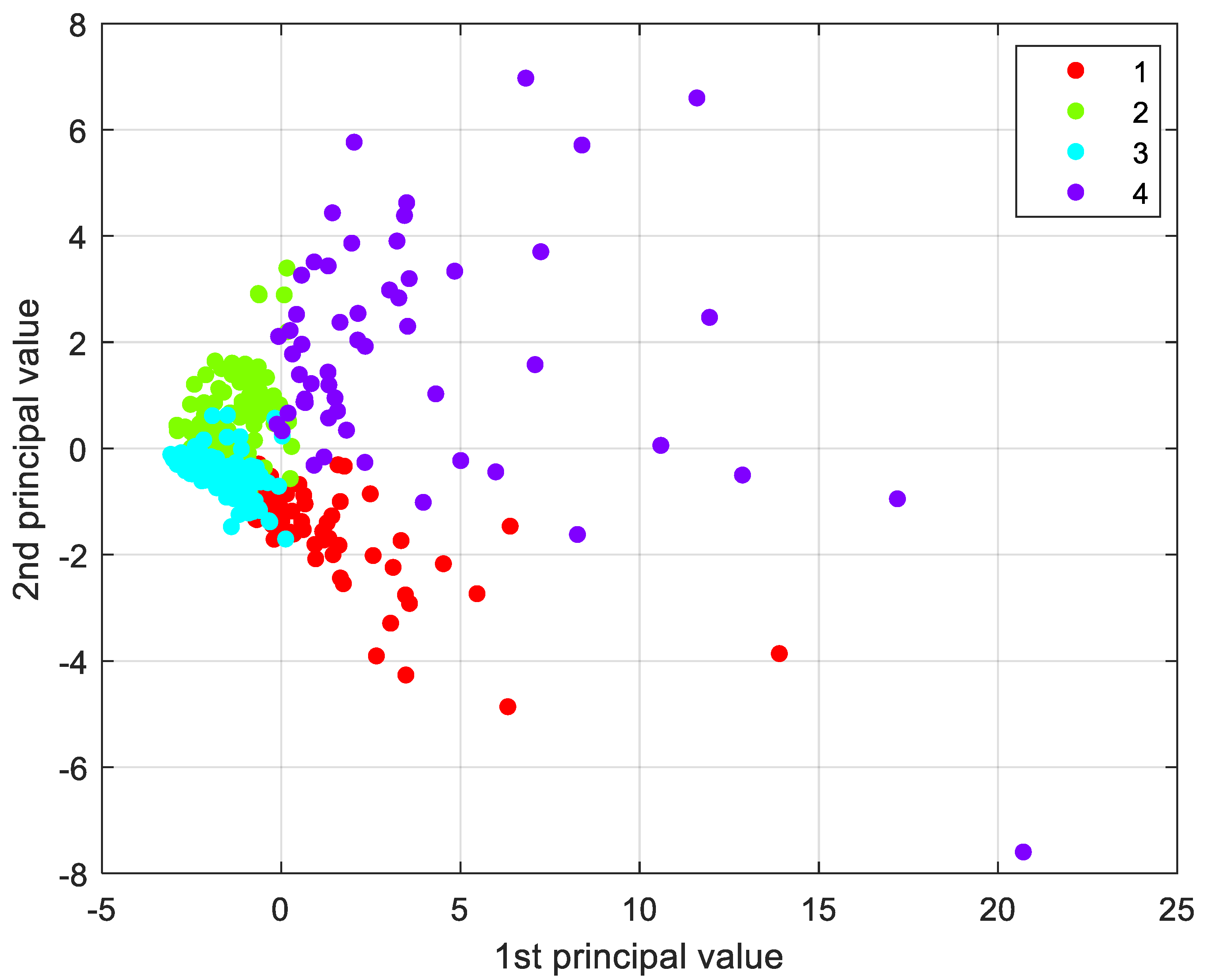
Once the dimension of the dataset has been reduced, it is possible to plot the observations in the new space generated by the principal components, space where the coordinates of the observations have undergone linear transformation, in accordance with the variables as mentioned before.

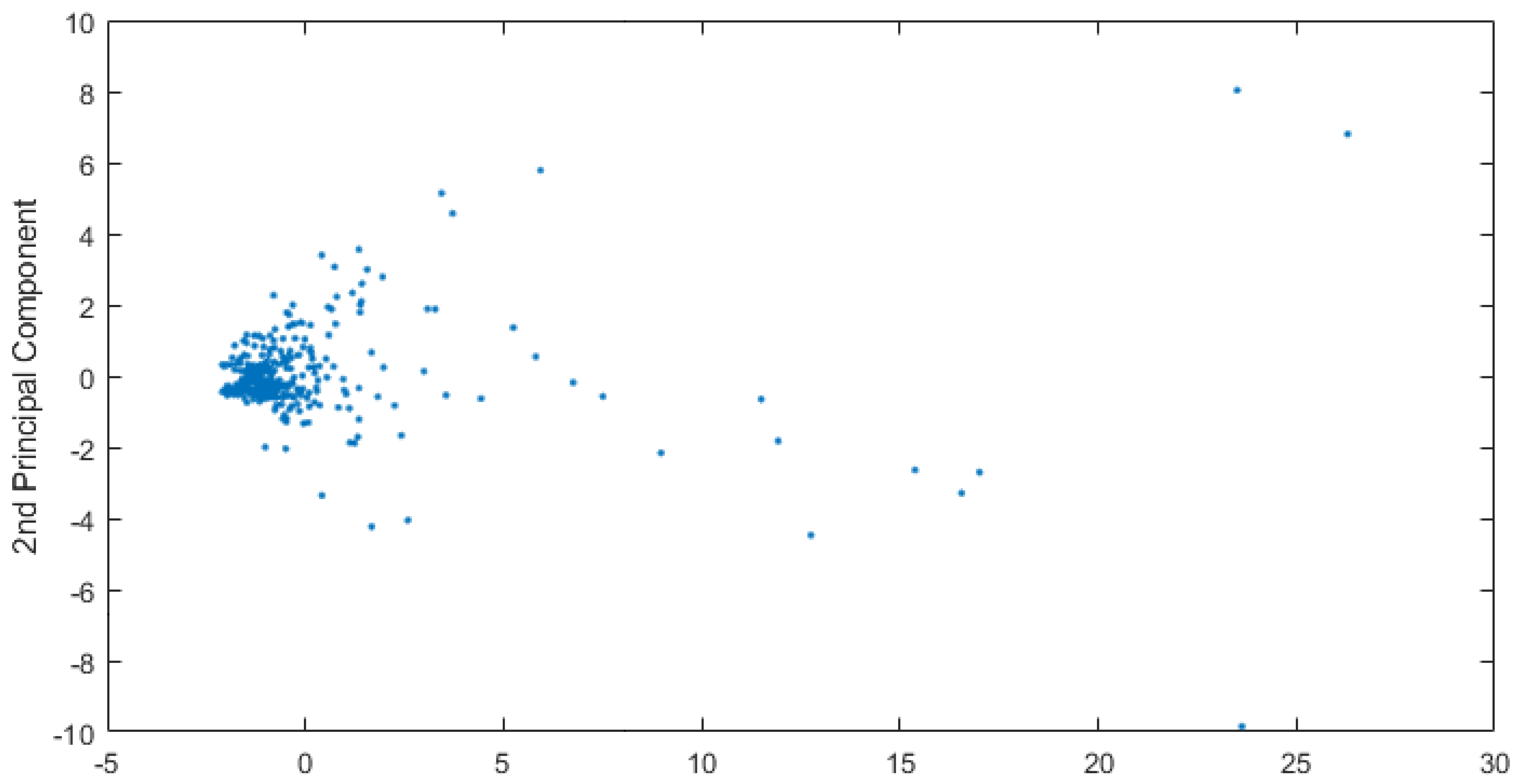
The scatter plot represented in Figure 3, depicts the observations after variable reduction. One can notice the presence of elements defined as outliers, i.e., abnormal values, far from the average observations. These disturbing elements could generate unbalanced compensations inside the analytical model, and that is why they will be handled with care, modifying the algorithm’s settings whenever possible or, in extreme cases, removed from the dataset. In this case, the outliers were almost all the administrative centers of Emilia-Romagna region, far away, in terms of the quantitative variables, from the rest of the observations.

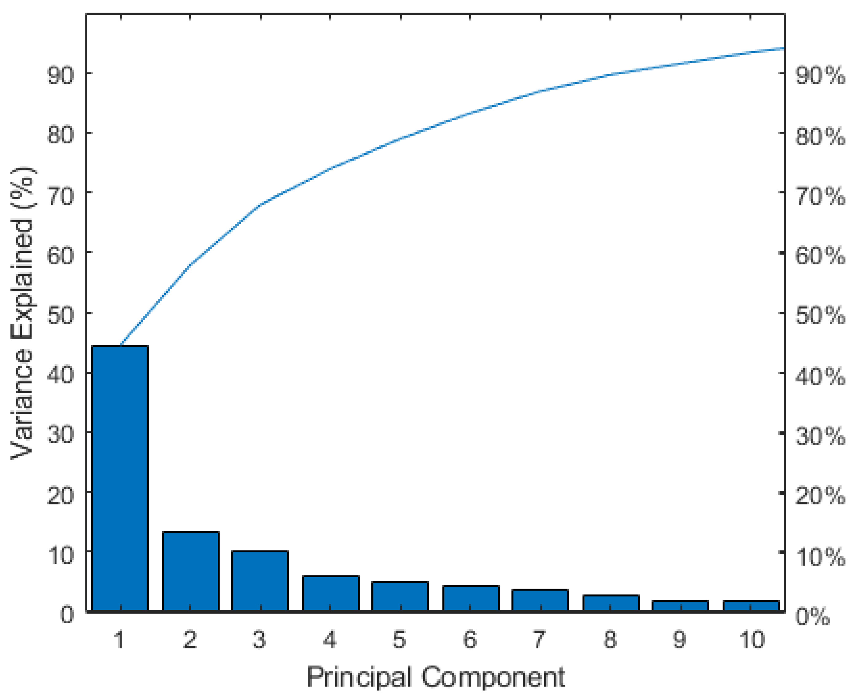
It is a good rule to consider the principal components that catch at least 80% of the variance of the starting dataset. The more the considered variables, the higher the number of principal components necessary to reach that quote. Whenever the amount of variance reached is not sufficient, an additional reduction in variables is performed by iterating the process.

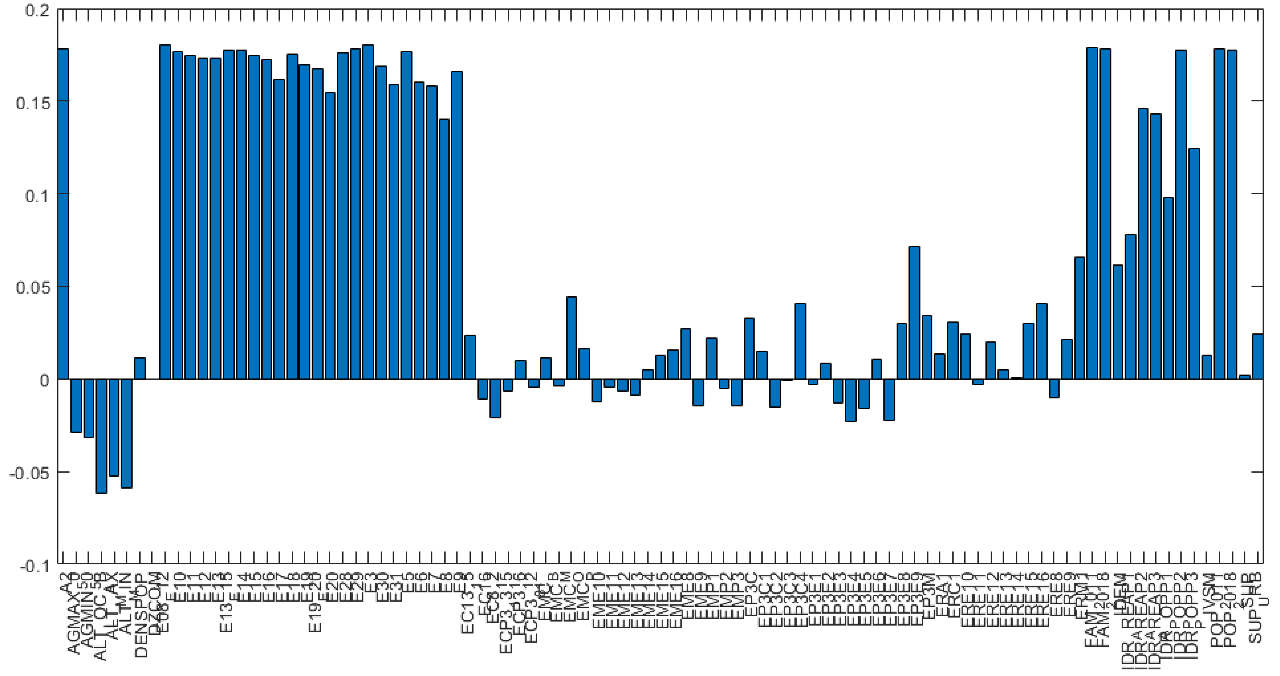
One of PCA’s main purposes is to delete the noise due to non-useful data, which is evaluated in terms of how much information and how much variance they carry inside the dataset. Figure 4 represents variance for each principal component before variable reduction. Loading plots have been generated as histograms representing the weight of the variables transformed after the PCA and are reported in Figure 5 and Figure 6. The variables reported along the abscissa have been selected among all the available data for being the most meaningful as per the multi-risk evaluation. For instance, AGMAX_50 denotes the maximum ground acceleration (fiftieth percentile) calculated on a grid with a 0.02° step, with the maximum and minimum of the values of the grid points falling within the municipal area. IDR_POPP3 indicates the resident population at risk in areas with high hydraulic hazard (P3). 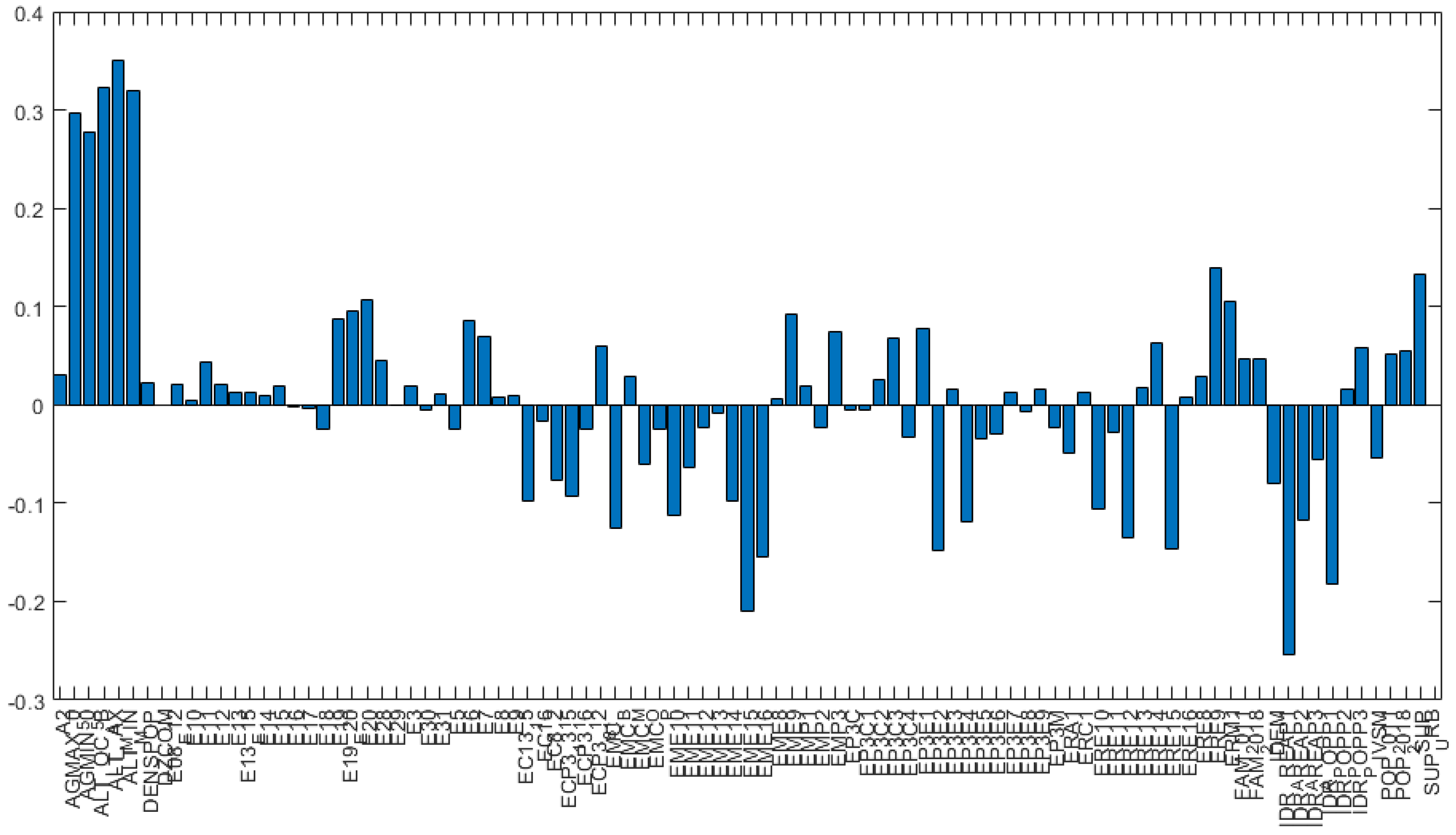From Figure 5 and Figure 6, the variables with the highest coefficients have been extrapolated, the higher the coefficient of the variable, the higher the weight of the variable on the principal component. Along the first principal component, the difference between observations will be led by the different values referred to the variables with highest coefficient in the histogram depicted in Figure 5.

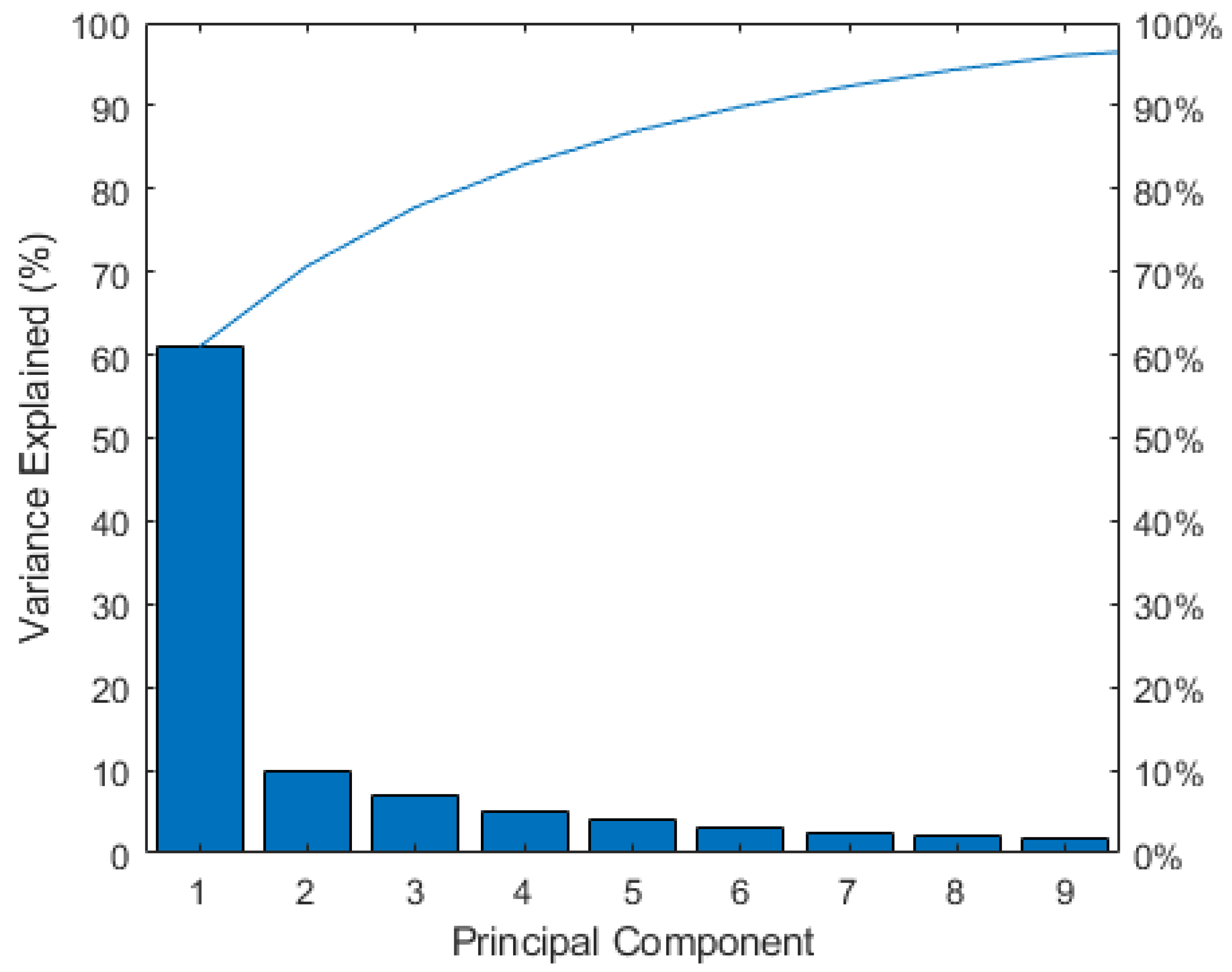
We chose to assess the weight of the coefficient of the variables referring to the first two principal components only, because they explicated more than 70% of the variance and are the most significant of the combined risk assessment. Figure 7 depicts the variance explicated by the first 10 principal components after the PCA.

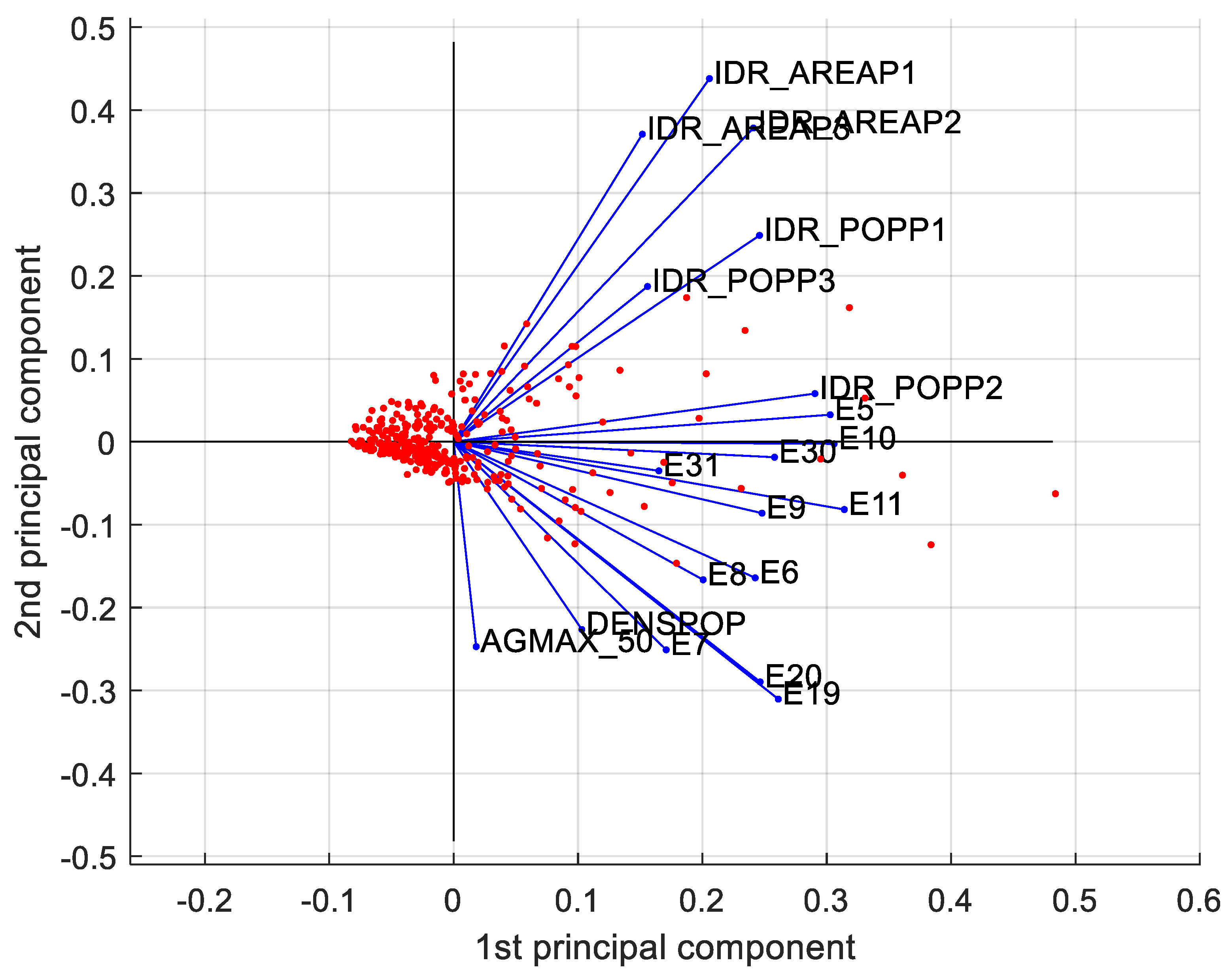
Fundamental to the visualization of both observations and the relation between the variables is the biplot in Figure 8.

This plot allows catching at an early stage any pattern within the dataset, such as the separation between observations and deep relation among variables. In general:

• the projection of the values on each principal component shows how much weight those values have on that principal component;
• when two vectors are close, in terms of angle, the two represented variables have a positive correlation;
• if two vectors create a 90 angle, the respective variables are not correlated;
• when they diverge and create an angle of almost 180, they are negatively correlated.

Outliers differ from the other observations in terms of vulnerability and the population at hydraulic risk. It is reasonable because, remembering the outliers are the provincial administrative centers, they present higher values in terms of population and built environment. Moreover, along the vertical axis the observations differ in terms of seismic hazard and exposition.

Moreover, vulnerability and exposure to hydraulic risk variables are quite correlated and differentiate the observations along the horizontal axis, whereas seismic hazard and exposition variables are not correlated with the variables representing surfaces at hydraulic risk. These remarks will come in handy later, at a post-clustering stage, a level of multi-risk will be attributed to each cluster.

2.3. K-Means Clustering Algorithm

The PCA allowed us to reduce the dimensionality of the dataset and plot the observations, i.e., the municipalities of the Emilia Romagna region, in the new sub-space identified by the principal components, while retaining the majority of information, which identified the observations in the initial n-dimensional space before the linear transformations.

To suitably group the observations according to homogeneous levels of overall risk, we used an unsupervised machine learning algorithm, known as k-means clustering.

In general, cluster analysis is a technique to group data where the main purpose is to gather observations according to the features selected by the user. The analysis allows splitting a set of observations into clusters according to similar or non-similar features. Cluster analysis does not require knowing the classes in advance, as in the case of supervised algorithms.

In the k-means clustering algorithm, we assumed $N$ observations $x_1,x_2,\dots ,x_n$ and partitioned them into $k$ clusters, each defined by a centroid $c_1,c_2,\dots ,c_k$. We assigned the $x_i$ observation to the cluster, such that the distance among the observation and the cluster center was minimum.

The algorithm began by randomly choosing k centroids. After measuring the distance of each observation to each centroid, the observation was assigned to the closest cluster. Then, centroids were updated, as the average of the observations in each centroid. The procedure was repeated iteratively, each time minimizing the distance between observation and centroid.

Different choices for such distance function are possible and readily available in many scientific computing software packages such as MATLAB: the squared Euclidean distance, one minus the cosine of the included angle between points (treated as vectors), or one minus the sample correlation between points (treated as sequences of values).

In particular, the squared Euclidean metric does not allow keeping the outlier in the dataset because of the square of the distance. By doing so, the algorithm will place a specific cluster just for the outlier, influenced by its distance from the other observations. Later, we will propose a comparison among the distances in terms of the quality of clustering.

To legitimate the clusterization carried out with the k-means algorithm, the silhouette method was employed. The technique provided a succinct graphical representation of how well each observation has been classified. The silhouette value is a measure of how similar an object is to its own cluster (cohesion) compared to other clusters (separation). The silhouette ranges from −1 to +1, where a high value indicates that the object is well matched to its own cluster and poorly matched to neighboring clusters. If most objects have a high value, then the clustering configuration is appropriate. If many points have a low or negative value, then the clustering configuration may have too many or too few clusters. The silhouette can be calculated with any distance metric, such as the Euclidean distance or the so-called Manhattan distance.

To decide which metrics to adopt, a comparison based on the silhouette of each method was performed (see Figure 9). Correlation metrics appear to be the most reliable, whereas the squared Euclidean would be as good if it were not for the outliers.

A four clusters grouping was chosen for the proposed analysis. Figure 10 represents the final clusterization of Emilia-Romagna municipalities. Cluster evaluation was conducted considering the weight and the distribution of the variables. All the outliers belonged to cluster 4, which was developed both on the horizontal axis, led by seismic vulnerability and hydraulic risk variables, and slightly on the vertical one, led by seismic hazard and by hydraulic risk variables. The great majority of the municipalities presented similar quantitative values of variables, in particular, those belonging to clusters 2 and 3. Silhouette values relative to this clusterization were good, reinforcing the reliability of the method proposed.

3. Results

In this section, we show how to assign to each observation and, more generally, to each cluster, a label which identifies the associated level of overall risk.

3.1. Variables Label Assignment

First, we set intervals in an objective way, in order to suitably define labels for the variables. To this aim, we set interval extremals in correspondence of quartile percentages Q1, Q2, and Q3 as indicated in

Table 1. Labels and intervals for cluster definition.

Intervals	Label
first element: Q1	Low
Q1: Q2	Medium-to-low
Q2: Q3	Medium-to-high
Q3: last element	High

.

The chosen labels referred, respectively, to the presence of low, medium-to-low, medium-to-high and high amounts regarding that specific variable. Such subdivision was allowed because the variables were quantitative types and sorted by normal distribution. Furthermore, sorting out variables, the information within them was unaffected.

We analyzed the variable with the greater value from the previous analysis, as a component that defined a risk, with the risk as the combined result of three factors, hazard, exposure, and vulnerability. We illustrate how to assign a label to each cluster for each variable considered, among the most relevant ones.

We first considered the variable $a_{g,max}$, i.e., the peak ground acceleration for the site, with a return period of 475 years. The first step was the extrapolation of observables in the initial dataset. Subsequently, we associated each observation with the respective cluster indexes and the respective values of $a_{g,max}$. Then, we rearranged the observables in ascending order of $a_{g,max}$, and defined the quartile as the extreme point of the interval. The cluster composition in terms of $a_{g,max}$ is reported in

Table 2. Quartile distribution of the $a_{g,max}$ variable in the four clusters.

	%Q1	%Q2	%Q3	%Q4	Label
CL1	74	20	6	0	Low
CL2	0	25	25	50	Medium-to-high
CL3	3	18	68	11	Medium-to-low
CL4	7	16	13	64	High

, together with the resulting assigned labels.

The labels were assigned based on the percentage prevalence of the cluster for each quartile. A prevalence allocated in the fourth quartile for one of the clusters indicated that the selected cluster gathered the most dangerous municipalities in terms of $a_{g,max}$ On the other hand, a prevalence in the first quartile indicated that the cluster gathered the less dangerous municipalities in terms of seismic hazard.

The same operation was carried out for the hydraulic risk component IDR_POPP2, the prevailing seismic vulnerability variable, i.e., the percentage of buildings under poor maintenance conditions E_30, and the main exposure variable, i.e., density population DENS_POP (see

Table 3. Quartile distribution of the IDR_POPP2 variable in the four clusters.

	%Q1	%Q2	%Q3	%Q4	Label
CL1	17	20	54	9	Medium-to-low
CL2	46	41	12	1	Low
CL3	3	5	18	74	Medium-to-high
CL4	4	5	9	82	High

,

Table 4. Quartile distribution of the E_30 variable in the four clusters.

	%Q1	%Q2	%Q3	%Q4	Label
CL1	41	27	22	9	Low
CL2	25	30	29	15	Medium-to-low
CL3	18	29	37	16	Medium-to-high
CL4	0	4	11	86	High

and

Table 5. Quartile distribution of the $a_{g,max}$ variable in the four clusters.

	%Q1	%Q2	%Q3	%Q4	Label
CL1	16	29	40	14	Medium-to-low
CL2	46	28	19	7	Low
CL3	0	0	3	97	High
CL4	5	25	27	43	Medium-to-high

).

3.2. Overall Risk Definition

Once the variables were rearranged, the incidence of clusters for each variable were calculated and a label for each variable and cluster was assigned (based on the distribution of the cluster indexes within the variable); each cluster was assigned an overall risk label based on their score for each rearranged variable (

Table 6. Overall risk quantification for each cluster of municipalities.

	Hydraulic Risk	Seismic Exposition	Seismic Vulnerability	Seismic Hazard	Label
CL1	Medium-to-low	Low	Medium-to-low	Low	Low
CL2	Low	Medium-to-low	Low	Medium-to-high	Low-to-medium
CL3	Medium-to-high	Medium-to-high	High	Medium-to-low	Medium-to-high
CL4	High	High	Medium-to high	High	High

).

The significance of the assigned risk labels was strictly dependent on the starting population, i.e., from the region under study and do not have absolute value.

This means that the obtained labels cannot be extrapolated to a larger scale without losing their significance. As shown in Figure 11, it is also possible to represent the population of each risk cluster by the main administrative province in the Emilia Romagna region. Obviously, frequency values for each province depend on the number of municipalities, which constitute each province. Therefore, this plot allows analyzing risk clusters from the same province, but comparing clusters from different provinces may be inappropriate. It is worth noting that the proposed methodology has recognized Piacenza as the province with most low-risk municipalities, while the main cluster featuring Parma, Modena, Bologna, Forlì-Cesena, and Rimini is the low-to-medium risk cluster. Most municipalities of the Reggio-Emilia province are associated with low and low-to-medium clusters. Finally, each of the provinces of Ferrara and Ravenna result being equally split in two main clusters, namely the low and the high-risk clusters in the former case, and the low-to-medium and high-risk clusters in the latter case.

4. Discussion

Ensuring ethical, inclusive, and unbiased machine learning tools is one of the new epistemic frontiers in the application of artificial intelligence technologies to disaster risk management. We recall that this paper discusses an individual application of machine learning tools to a multi-risk assessment of a Northern Italy case study. For this purpose, we had at our disposal a massive amount of data from the ISTAT database containing indicators and data on seismic, hydrogeological, and volcanic risk as well as demographic, housing, territorial and geographical information, obtained through the integration of various institutional sources such as Istat, INGV, ISPRA, Italian Ministry for Cultural Heritage. Like all big data technologies, the adopted machine learning model proved effective in reducing CPU time and model-development costs, owing to its ability to process quantities and sources of data that could not have been otherwise simply elaborated [24,25]. We expect that the model can be used to devise mitigation measures, prepare emergency response, and plan flood recovery measures. The proposed tool has, indeed, the potential for being an operational instrument for land use managers and planners. However, misuse should be avoided, and, for this purpose, crucial issues such as applicability, bias, and ethics should be carefully considered [24,25,26]. The ethical issues pertaining to a possible misuse of Artificial Intelligence technologies are several [25], including the loss of human decision making, the potential for criminal and malicious use, the emergence of problems of control and use of data and systems, the dependence of the outcomes on users’ bias, and the possible prioritization of the “wrong” problems with respect to stakeholder expectations.

Prioritization in disaster multi-risk management, additionally, is markedly affected by needs and expectations of private users, public agencies, and final stakeholders. For instance, a water level management company will be expectedly more inclined to consider flood risk as the most important risk to cope with, while any public agency that is called to reduce the seismic vulnerability of a certain region will tend to consider seismic risk as a priority. Thus, the labeling of the clusterization will be intrinsically permeated with the end-user’s intentions. A further aspect is that one should understand that publicizing the results of a multi-risk algorithm might inadvertently touch sensitive aspects from a privacy point of view [27].

In many cases, criticalities rely upon an inherent disconnect between the algorithm’s designers and the communities where the research is conducted [26], while users may complain about a lack of transparency and accountability. Furthermore, immature machine learning tools might be used in safety-critical situations for which they are not yet ready. As suggested by Gevaert et al. [26], disaster-risk-management specialists constantly seek expertise on how to clearly communicate the results and uncertainties of machine learning algorithms to reduce inflated expectations. Furthermore, sensitive groups should be identified and audited for overcoming bias. Therefore, we suggest that, before being systematically applied, the present machine learning methodology is validated against established computational modeling tools. We also believe that the obtained results are very promising, but further efforts are necessary to assess the proneness of the proposed machine learning tool to the aforementioned ethical and bias issues.

5. Conclusions

The purpose of this work is to illustrate a sound methodology for the qualitative multi-risk analysis at the regional scale by means of machine learning techniques that allow dealing with large and heterogeneous amounts of data. The initial dataset, made of variables carrying information about hazard, exposure, and vulnerability for both seismic and hydraulic risk for each municipality of the Emilia Romagna region, has been suitably normalized and reduced through the PCA, whereas observations have been clustered through a machine-learning algorithm.

Then, risk labels were individually assigned to clusters for each variable. Finally, based on the score of each variable an overall risk label was assigned to each cluster. Results confirmed previous risk classifications for the case study analyzed. Both provinces with a moderate risk level and high-risk level have been correctly detected by the proposed approach. The reliability of the obtained results is dependent on the existence of valid quantitative initial data for the region under study. In fact, the proposed methodology does not allow qualitative data, whether they are fundamental or not.

In conclusion, the proposed analysis delivers useful information: municipalities with major priority of intervention are identified so that stakeholders can take advantage of this tool to prioritize any preventive measures. Moreover, the procedure also allows identifying the most important variables to consider in a combined seismic and hydraulic multi-risk analysis. In other words, this tool allows evaluating the variables most suited to categorize the observations in terms of combined risk. Indeed, from the analysis, variables have emerged relative to different types of risks, which better communicate with each other and carry most information. By contrast, the methodology also allows identifying variables, which do not collaborate with variables of different nature and, therefore, cannot be usefully employed.

References

1. Fuchs, S.; Keiler, M.; Zischg, A. A spatiotemporal multi-hazard exposure assessment based on property data. Nat. Hazards Earth Syst. Sci. 2015, 15, 2127–2142. [Google Scholar] [CrossRef] [Green Version]
2. Kron, W. Reasons for the increase in natural catastrophes: The development of exposed areas. In Topics 2000: Natural Catastrophes, the Current Position; Munich Reinsurance Company: Munich, Germany, 1999; pp. 82–94. [Google Scholar]
3. Zschau, J. Where are we with multihazards, multirisks assessment capacities? In Science for Disaster Risk Management: Knowing Better and Losing Less; Poljansek, K., Marin Ferrer, M., De Groeve, T., Clark, I., Eds.; European Union: Luxembourg, 2017; pp. 98–115. [Google Scholar]
4. Barthel, F.; Neumayer, E. A trend analysis of normalized insured damage from natural disasters. Clim. Chang. 2012, 113, 215–237. [Google Scholar] [CrossRef] [Green Version]
5. Munich, R.E.; Kron, W.; Schuck, A. Analyses, assessments, positions. In Topics Geo: Natural Catastrophes; Münchener Rückversicherungs-Gesellschaft: Munich, Germany, 2014. [Google Scholar]
6. Peduzzi, P.; Dao, H.; Herold, C.; Mouton, F. Assessing global exposure and vulnerability towards natural hazards: The Disaster Risk Index. Nat. Hazards Earth Syst. Sci. 2009, 9, 1149–1159. [Google Scholar] [CrossRef]
7. Bell, R.; Glade, T. Multi-hazard analysis in natural risk assessments. WIT Trans. Ecol. Environ. 2004, 77, 1–10. [Google Scholar]
8. Barredo, J.I. Major flood disasters in Europe: 1950–2005. Nat. Hazards 2007, 42, 125–148. [Google Scholar] [CrossRef]
9. Kanamori, H.; Hauksson, E.; Heaton, T. Real-time seismology and earthquake hazard mitigation. Nature 1997, 390, 461–464. [Google Scholar] [CrossRef]
10. Kappes, M.S.; Keiler, M.; von Elverfeldt, K.; Glade, T. Challenges of analyzing multi-hazard risk: A review. Nat. Hazards 2012, 64, 1925–1958. [Google Scholar] [CrossRef] [Green Version]
11. Schmidt, J.; Matcham, I.; Reese, S.; King, A.; Bell, R.; Henderson, R.; Smart, G.; Cousins, J.; Smith, W.; Heron, D. Quantitative multi-risk analysis for natural hazards: A framework for multi-risk modelling. Nat. Hazards 2011, 58, 1169–1192. [Google Scholar] [CrossRef]
12. Gruber, F.E.; Mergili, M. Regional-scale analysis of high-mountain multi-hazard and risk indicators in the Pamir (Tajikistan) with GRASS GIS. Nat. Hazards Earth Syst. Sci. 2013, 13, 2779–2796. [Google Scholar] [CrossRef] [Green Version]
13. Tyagunov, S.; Vorogushyn, S.; Jimenez, C.M.; Parolai, S.; Fleming, K. Multi-hazard fragility analysis for fluvial dikes in earthquake- and flood-prone areas. Nat. Hazard. Earth Syst. Sci. 2018, 18, 2345–2354. [Google Scholar] [CrossRef] [Green Version]
14. Yousefi, S.; Pourghasemi, H.R.; Emami, S.N.; Pouyan, S.; Eskandari, S.; Tiefenbacher, J.P. A machine learning framework for multi-hazards modeling and mapping in a mountainous area. Sci. Rep. 2020, 10, 12144. [Google Scholar] [CrossRef] [PubMed]
15. Boniolo, F.; Dorigatti, E.; Ohnmacht, A.J.; Saur, D.; Schubert, B.; Menden, M.P. Artificial intelligence in early drug discovery enabling precision medicine. Expert Opin. Drug Discov. 2021, 16, 991–1007. [Google Scholar] [CrossRef]
16. Pouyan, S.; Pourghasemi, H.R.; Bordbar, M.; Rahmanian, S.; Clague, J.J. A multi-hazard map-based flooding, gully erosion, forest fires, and earthquakes in Iran. Sci. Rep. 2021, 11, 14889. [Google Scholar] [CrossRef] [PubMed]
17. Pearson, K. On Lines and Planes of Closest Fit to Systems of Points in Space. Phil. Mag. 1901, 2, 559–572. [Google Scholar] [CrossRef] [Green Version]
18. Hotelling, H. Analysis of a complex of statistical variables into principal components. J. Edu. Psychol. 1933, 24, 417–441. [Google Scholar] [CrossRef]
19. Jolliffe, I.T. Principal Component Analysis; Springer: New York, NY, USA, 2002. [Google Scholar]
20. MacQueen, J.B. Some methods for classification and analysis of multivariate observations. In Proceedings of the 5th Berkeley Symposium on Mathematical Statistics and Probability, Berkeley, CA, USA, 1967; University of California Press: Berkeley, CA, USA, 1967; pp. 281–297. [Google Scholar]
21. Ding, C.; Xieofeng, H. K-means clustering via principal components analysis. In Proceedings of the 21st International Conference on Machine Learning, Banff, AB, Canada, 4–8 July 2004; ACM Press: New York, NY, USA, 2004. [Google Scholar]
22. Trigila, A.; Iadanza, C.; Bussettini, M.; Lastoria, B. Dissesto Idrogeologico in Italia: Pericolosità e Indicatori di Rischio—Edizione 2018; Rapporti 287/2018; ISPRA: Roma, Italy, 2018. [Google Scholar]
23. Mantovan, L.; Gilli, A. Supplementary Material, Open Access. Available online: https://github.com/alessandrogilli/analisi-multirischio (accessed on 15 October 2021).
24. Wagenaar, D.; Curran, A.; Balbi, M.; Bhardwaj, A.; Soden, R.; Hartato, E.; Sarica, G.M.; Ruangpan, L.; Molinario, G.; Lallemant, D. Invited perspectives: How machine learning will change flood risk and impact assessment. Nat. Hazards Earth Syst. Sci. 2020, 20, 1149–1161. [Google Scholar] [CrossRef]
25. Stahl, B.C. Ethical Issues of AI. Artificial Intelligence for a Better Future: An Ecosystem Perspective on the Ethics of AI and Emerging Digital Technologies. In SpringerBriefs in Research and Innovation Governance; Springer: Berlin/Heidelberg, Germany, 2021; pp. 35–53. [Google Scholar]
26. Gevaert, C.M.; Carman, M.; Rosman, B.; Georgiadou, Y.; Soden, R. Fairness and accountability of AI in disaster risk management: Opportunities and challenges. Patterns 2021, 2, 100363. [Google Scholar] [CrossRef] [PubMed]
27. GFDRR. Machine Learning for Disaster Risk Management; GFDRR: Washington, WA, USA, 2018. [Google Scholar]
Figure 1. Seismic classification of municipalities in Emilia (https://ambiente.regione.emilia-romagna.it/en/geologia/seismic-risk/seismic-classification, accessed on 15 October 2021).
Applsci 12 00583 g001
Figure 2. Ferrara territory altimetry (The map can be downloaded from https://www.bonificaferrara.it and has been released from “Consorzio di Bonifica Pianura di Ferrara”; accessed on 15 October 2021).
Applsci 12 00583 g002
Figure 3. Observations scatter plot which depicts the observations after variable reduction.
Applsci 12 00583 g003
Figure 4. Variance for each principal component before variable reduction.
Applsci 12 00583 g004
Figure 5. Loading plot of the variable coefficients along the first principal component (see Appendix A for an explanation of the acronyms).
Applsci 12 00583 g005
Figure 6. Loading plot of the variables coefficients along the second principal component (see Appendix A for an explanation of the acronyms).
Applsci 12 00583 g006
Figure 7. Variance of the first 10 principal components after variable reduction.
Applsci 12 00583 g007
Figure 8. Biplot along the first two principal components.
Applsci 12 00583 g008
Figure 9. Silhouette for different metrics: squared Eculidean (a), cosine (b), and correlation (c).
Applsci 12 00583 g009
Figure 10. Grouping of the Emilia Romagna municipalities into four clusters.
Applsci 12 00583 g010
Figure 11. Population of each risk cluster by province in the Emilia Romagna region. In the y-axis, the number of municipalities has been reported.
Applsci 12 00583 g011