
Turbulent Flow over Confined Backward-Facing Step: PIV vs. DNS
by
 and
and
Boštjan Zajec
*, 
Marko Matkovič
,
Nejc Kosanič
,
Jure Oder
,
Blaž Mikuž
,
Jan Kren
and
Iztok Tiselj
* Jožef Stefan Institute, Jamova Cesta 39, SI-1000 Ljubljana, Slovenia
*
Authors to whom correspondence should be addressed.
Appl. Sci. 2021, 11(22), 10582; https://doi.org/10.3390/app112210582
Submission received: 22 September 2021
/
Revised: 5 November 2021
/
Accepted: 6 November 2021
/
Published: 10 November 2021
(This article belongs to the Section Fluid Science and Technology)
Abstract
:Featured Application
The paper answers the question about an expected agreement between the very accurate numerical simulations and very accurate experiments in 3D time-averaged turbulent flow with separation.
Abstract
Particle Image Velocimetry measurements of the liquid velocity fields in the flow over the backward-facing step were performed in the same flow configuration as in the existing Direct Numerical Simulation (DNS). The experiment and the simulation were performed in an identical cross-section geometry with step expansion rate 2.25 and the square shape of the outlet duct at the Reynolds number in an inlet part of the section 7100. The experiment was performed in transparent test section, 1.2 m long, with 20 × 45 mm2 cross-section upstream and 45 × 45 mm2 downstream, while a domain that was three times shorter was used in the DNS. A 2D-2C PIV system with a single high-speed camera and a pulse laser was used for a series of two-dimensional measurements of the velocity field at several cross-sections from two different perspectives. Variables analyzed in the experiment are time-averaged fluid velocities, velocity RMS fluctuations and two components of the Reynolds stress tensor. The key novelty is the comparison of two very accurate approaches, PIV and DNS, in the same cross-section geometry. Comparison of the similarities, and especially the differences between the two approaches, elucidates uncertainties of both studies and answers the question on what kind of agreement is expected when two very accurate approaches are compared.
1. Introduction
The separation and reattachment of turbulent flows occur in many industrial applications and natural systems, and as such, represent an important field of study. Flow over a Backward-Facing Step (BFS) is one of the simplest geometries with flow separation, recirculation, and reattachment and as such, is a representative geometry for sudden expansions in pipes, channels and ducts. Simple geometry means that it can be easily studied in experiments and modelled with computational fluid dynamics. As such, the channel with a step represents a next step in complexity compared to the flows through the constant cross-section ducts and channels. Flows in BFS geometry are important because flow separation drastically increases the momentum, heat and mass transfer downstream the step. According to a recent review study on separated flows by Terekhov [1], the flow behind a backward step is one of the cases which attracted the most attention in the available literature.
The BFS geometry considered in the present study was chosen as one of the reference geometries within the EU-EURATOM research project SESAME (2015–2019), which aimed at experimental and computational research of liquid metal flow and heat transfer. Among the results of the SESAME project is an extensive DNS study performed by Oder et al. [2], which considers the heat transfer in the liquid metal flow through BFS geometry. The key novelty in [2] is the 3D nature of the recirculating flow behind the step, which is a consequence of BFS confinement in a spanwise direction. The temperature field of Oder’s study is a passive scalar; thus, the velocity fields allow comparison with adiabatic experiments that can be performed with water. The BFS geometry in SESAME project was considered in a liquid metal experiment [2] at the same Reynolds number 7100, which included the heated section at the same position as in DNS of Oder et al. [2]. Such low Reynolds numbers are relevant for liquid metal reactors [3], where low flow rates are foreseen due to the superb heat transfer characteristics of the coolants. Since the final geometry and the Reynolds number of liquid metal experiment [4] were slightly different than in DNS, the second BFS experiment related to the SESAME project was developed: adiabatic experiment performed with water and without heating. This experiment is described in the present paper.
When the spanwise dimension of the BFS geometry is at least ten step heights wide, the flow behind the step can be treated as two-dimensional in time-averaged sense [5], which means that it contains another simplification comparing to the general sudden expansion geometry. Two-dimensional time-averaged BFS flows have been studied experimentally in many previous publications. Some of the early publications were written by Abbot and Kline [6] and De Brederode and Bradshaw [7]. More recent studies are those of Armaly et al. [8], Kasagi and Matsunaga [9], and Beaudoin et al. [10]. Relatively new studies were recently performed by Liakos and Malamataris [11], Buckingham [12], Chen et al. [13], Polewski and Cizmas [14], and Pont-Vilchez et al. [15]. Many of the previous studies were focused on the heat transfer behind the BFS expansion that might include natural or mixed convection cases [16]. Especially in nuclear engineering, studies are focused on heat transfer of liquid metal flows [12,17]. An extensive review of separated flows, including the BFS flows, has been recently performed by Terekhov [1]. The main analysis in previous paper was aimed at assessing the effect of external turbulence on the dynamics and thermal characteristics of the separated flow behind different obstacles and it has been shown that turbulence of the incoming flow has a more noticeable effect on separated flows than on the boundary layers. At the same time, the turbulence upstream the BFS is not correlated with high turbulence induced in the shear layer of the separated flow [18,19,20]. Moreover, coherent vortex structures have been proved to exist in the separation-reattachment process downstream a backward-facing step flow with a Reynolds number of 4400 and 9000 [21]. They are well-organized in the recirculation regions with forming, developing, shedding, and redeveloping in the shear layer. Understanding the flow behavior is necessary for accurate modeling of such flows.
For a detailed review of the numerical studies of BFS geometry, the reader is referred to the paper by Oder et al. [2], where highly accurate numerical simulations performed with DNS and LES approaches are summarized. Here, we mention only the earliest DNS study in BFS geometry by Le et al. [22], while several recent publications are focused on more special configurations [2,15,23].
In this paper, we emphasize the studies which are relevant for our setup and deal with 3D time-averaged flows, where spanwise dimension of the duct with BFS is comparable with the step height. The shape of the recirculation vortices downstream the step has a complex 3D geometry, which presents an additional challenge for measurements and simulations. Lim et al. [24] performed experiments on the backward-facing step flow of air through a rectangular duct with an aspect ratio of 3.3 and expansion ratio of 2.0 at a Reynolds number of 10,000. They found that the reattachment length in 3D cases is smaller than in 2D. Velocities were measured with Laser-Doppler velocimetry and hot wire anemometry. Nie et al. [25] performed LDV measurements on air flowing over a BFS with an aspect ratio of 2 over a range of Reynolds numbers between 100–8000 with a special focus on reversed flow regions. Piirto et al. [26] performed PIV measurements on water flowing in a square duct with a BFS expansion ratio of 1.25 with Reynolds numbers between 12,000 and 55,000. They have confirmed the reattachment lengths that are smaller for 3D flows than in 2D.
The key parameter of the BFS geometry is its expansion ratio, i.e., the ratio of channel cross sections downstream and upstream of the backward step. Several experimental and numerical studies in BFS geometries have been performed with different Reynolds numbers, channel shapes and expansion ratios. Most of them at expansion ratios close to 1, while the geometries with ratios around 2 are rather scarce [13,15,27]. The DNS data of Oder et al. [2] served as a starting point for experimental part of the research described in this paper. We have not found the specific cases of the rectangular channel with expansion ratio of around 2 and with moderate Reynolds numbers, which can be accurately described with DNS (or LES) studies. Since such a numerical study was performed by Oder et al. [2], we decided to build a test-section based on this simulation. The first preliminary experimental results with velocities measured in a single plane were presented by Zajec et al. [28] and represent the first PIV measurements performed in our laboratory. The present PIV results are obtained in a new test section at Reynolds number 7100, which corresponds to the Reynolds number of the simulation.
While DNS results are often treated as perfect and are assumed to contain no errors except the statistical uncertainty of the realized turbulent flow, even DNS data are not entirely immune to systematic errors, which can only be exposed with accurate measurements. The new PIV study of the 3D BFS turbulence presents an added value in the field of turbulence studies. Comparison of PIV and DNS presents a mutual verification of both approaches and demonstrates their accuracy and their uncertainties. These data will be applicable for the assessment and development of LES and RANS models [29], which do not solve the smallest turbulent scales explicitly, but consider them with (semi)empirical turbulence models. Especially the RANS models remain the key tool for high Reynolds number industrial flows [30], where DNS approaches are typically not feasible and even LES models are too expensive due to the enormous computational power required.
2. Experimental and Computational Geometry
The first test section used in our laboratory by Zajec et al. [28] in 2018 was 1 m long. The most recent test section, used for measurements in the present paper, is 1.2 m long. The length, pump flow rate and the desired Reynolds number constrains resulted in a duct with inlet section with 45 × 20 mm2 cross-section, a step height of 25 mm, and a square duct of 45 × 45 mm2 downstream the step. The geometry has an expansion ratio of 2.25.
The part of the section downstream the step was extended from 32 cm in the first test section to 52 cm in the second and the third test section in order to diminish the effects of the constriction at the outflow, where the section is connected to a pipe with a diameter of 10 mm.
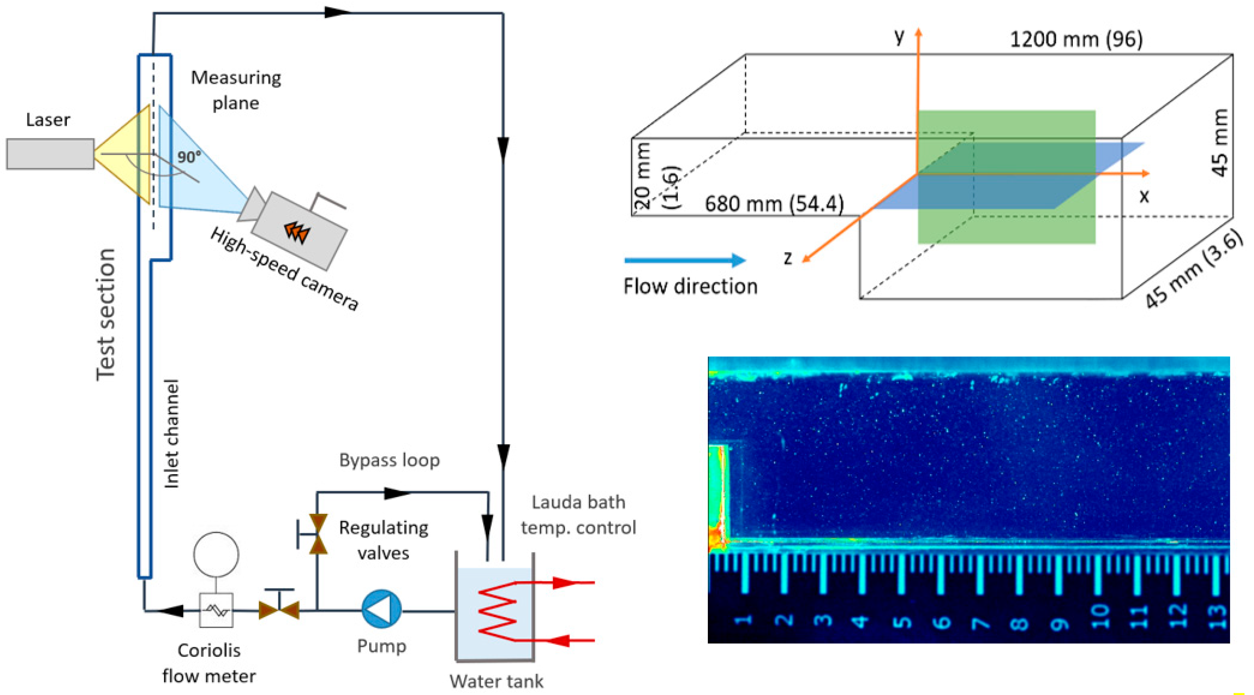
The complete backward-facing step test section, schematically shown in Figure 1, was manufactured from 10 mm thick polycarbonate plexiglass, to provide the transparency needed for PIV measurements. Water was used as a working fluid at a temperature of 24 ± 0.5 °C in order to minimize the variations of viscosity. The test section was positioned vertically and plumbed as a semi-open (non-pressurized) loop. Pump operating at constant flow rate was delivering water into the test section and into the by-pass loop. A valve was used for accurate setting of the mass flow rate through the main loop. The Coriolis flowmeter (Emerson Micro Motion) was used to measure the mass flow rate with an accuracy of 0.5% of the measured value. The Reynolds number, based on the hydraulic radius of the inflow and the bulk velocity at the inflow was equal to 7100. Fluctuations of the Reynolds number 7120 ± 20 were observed in the recorded histories of the mass flow rates during the measurement and are below the uncertainty of the flowmeter.
Each experimental case in Table 1 was performed with two separate measurements with position of the camera changed in x direction in each measurement. This approach improved the spatial resolution of each measurement in comparison with the first two experimental campaigns, but required an additional post-processing step where two measurements were merged in a streamwise direction. Small discontinuities are visible in the results of the measurements presented in several of the figures below for most of the cases in Table 1; nevertheless, this approach, with a reduced field of view, increased the spatial resolution of the measurements. The magnitude of the uncertainties related to the merging of images is closely related to the uncertainties of the camera position setting, image scaling and laser sheet position and is discussed in Section 4 and Section 5.
All figures and results are plotted in the dimensionless units of the DNS performed by Oder et al. [2] with dimensional units in the experiment converted into dimensionless values for comparison. The cross-section of the duct downstream the step is 3.6 × 3.6 dimensionless units, which corresponds to 45 × 45 mm2 in the experiment. The velocities are scaled with the bulk velocity in the upstream part of the test section, which was fixed to a unity value in the DNS, and corresponds to roughly 0.233 m/s inlet velocity in the experiment. Exact velocity used to convert measurements into dimensionless units took into account slight temperature and Reynolds number dependence separately for each measurement (~1% variations). Thus, the basic conversion between the dimensionless units and experiment are as follows:
- (a)
- 12.5 mm = 1 dimensionless length unit,
- (b)
- 0.233 m/s~1 dimensionless velocity unit.
3. Computational Set-Up of Direct Numerical Simulation
The DNS code Nek5000 [31] was used to solve dimensionless Navier-Stokes equations for incompressible fluid with internal energy equation. Details of the simulation, with a focus on heat transfer, are described in [2]. Since the passive scalar heat transfer equations do not affect the velocity field, they are irrelevant for the present work. The code Nek5000 is based on the spectral element method. Similar to the finite element method, the domain was divided into elements. Within each element, a spectral method was used to search for the solution. In this way, the method can be applied to irregularly shaped geometries, which are usually simulated with the finite element method. However, the spectral element method retains the quick convergence rate and the high accuracy of the spectral method. In addition, the elements serve as the unit for parallelization.
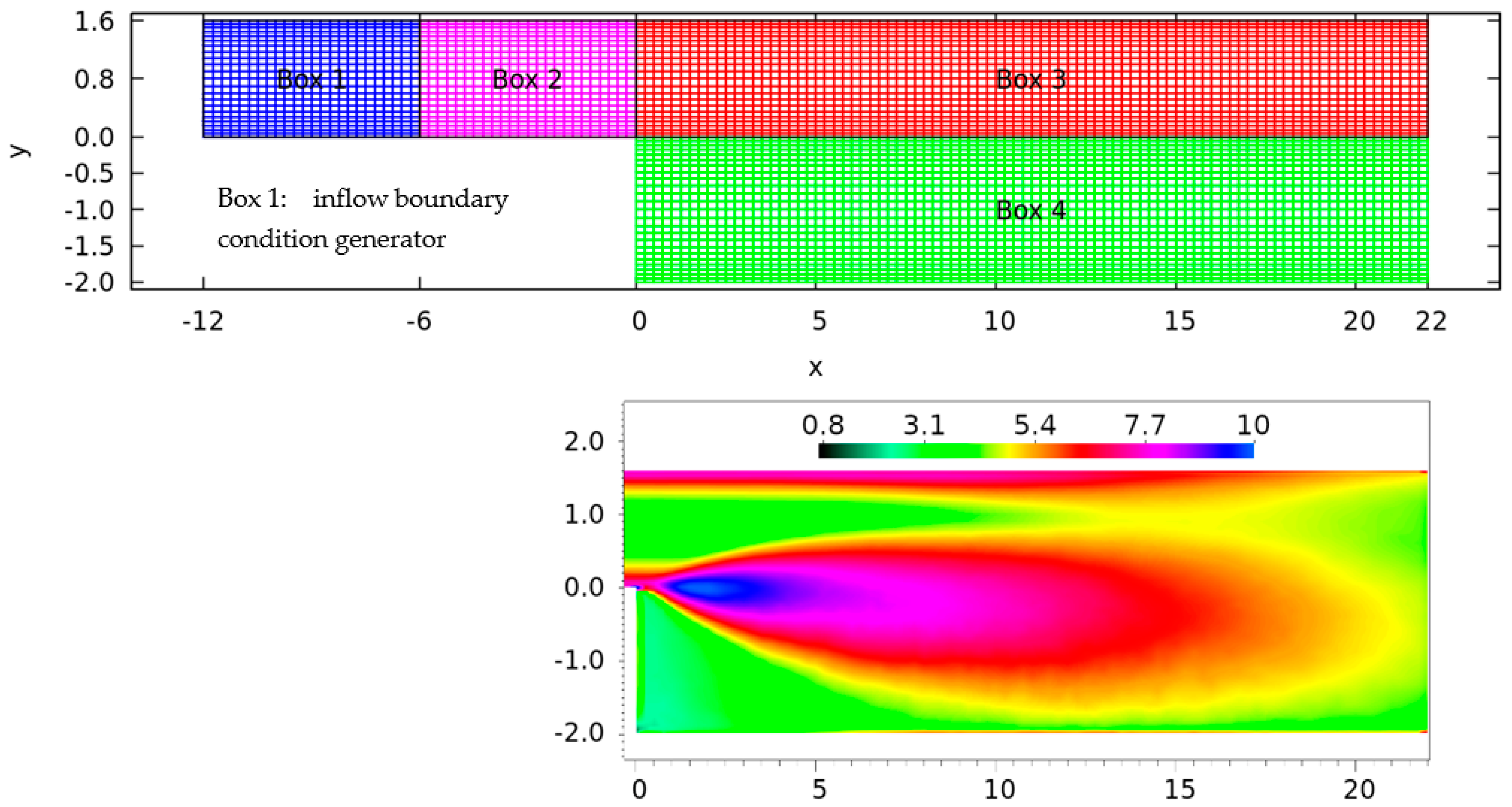
The computational domain in the DNS shown in Figure 2 is shorter than the one shown in Figure 1. A four-fold shorter inlet of 12 dimensionless units was applied and half of that inlet length was used to produce the fully developed turbulent inflow with the cyclic boundary condition. The inlet boundary condition ensured a constant mass flow rate through the domain. The outlet section in the computation was shorter too (22 dimensionless units); however, it was long enough to eliminate the influence of the outflow boundary condition on the recirculation vortex behind the step.
The computational domain was divided into approximately 153,000 elements, shown in the top drawing of Figure 2. The sizes of the elements varied in the wall normal directions and were smaller near the wall. However, the elements were of the same length in the streamwise x direction. Within each element, seven collocation points were used in each direction, bringing the number of points within each element to 343. Distances between the collocation points in the domain were in the following intervals: Δx Є [0.0212, 0.0586], Δy Є [0.0037, 0.0269] and Δz Є [0.0040, 0.0493]. These points define the basic cells but are not shown in Figure 2. The points on the boundaries between the elements coincided, so the total number of unique points within the domain was approximately 31 million.
The spatial resolution of the simulation is shown in the bottom drawing of Figure 2, where the ratio of the mesh cell and the local Kolmogorov scale, a posteriori obtained from the DNS results, is shown. Such a resolution is typical for DNS in 3D geometries.
The second-order accurate time integration is a combination of an explicit Adams-Bashfort scheme for convective and source terms and a semi-implicit backward differentiation for diffusion terms. The time step of 0.0004 dimensionless time units corresponds to around 10% of the CFL (Courant-Friedrichs-Lewy condition). Our tests have shown that the time step must be significantly lower than the stability limit of 0.5 CFL in order to ensure time step-independent results.
Since the domain was three-dimensional with walls surrounding the BFS, there were no homogeneous directions. This meant that no spatial averaging can be employed to ease the averaging procedure, except for the symmetry in the spanwise (z) direction, and DNS required long time-averaging intervals. The presented results are shown with averaging over about 4900 dimensionless time units or approximately 12 million time steps (3 million Intel Xeon-E5 CPU hours). The averaging time corresponds to roughly 80 flow-through times of the DNS domain. This is an order of magnitude more than in comparable studies, which had periodic boundary conditions in the spanwise direction and compensate the shorter averaging times with spatial averaging over the spanwise direction. Nevertheless, the statistical uncertainties due to finite averaging time are still important and are estimated to be around 1–2% percent in the average streamwise velocity, while for the RMS fluctuations, the uncertainties are estimated to be two times higher than for average velocities [2,32].
4. PIV Experiment and Data Processing
The PIV system consisted of an Nd:YLF double cavity pulsed laser (100 ns pulse) from Litron and a Phantom camera with a maximum resolution of 1280 × 800 pixels. With a Tokina 100 mm Macro F2.8 lens, we achieved a resolution of roughly 10 pixels per mm length and an active field of the images around 1250 × 450 pixels. To improve the resolution, flow downstream the step was measured in two separated runs, where each of them covered a streamwise length of around 13 cm. Both results were merged in the post-processing phase, where combined fields covered sufficient length to capture the flow behind the step up to the reattachment line, which is around 15–20 cm downstream the step. Camera positioning was performed with 3 mm (~2%) accuracy, which was roughly halved in the post-processing length calibration phase.
Hollow glass spheres with a diameter of 9–13 µm were dispersed in the water to provide particle seeds. With a density of 1.1 g/cm3 they are close to neutrally buoyant in water. PIV measurements of 2D velocity fields were performed in several planes, as described in Table 1. Two of these planes are also shown in the top-right drawing of Figure 1. The positions of the measured planes in Table 1 are given with respect to the origin of the coordinate system shown in Figure 1.
The laser sheet was around 1 mm thick. The laser sheet positioning uncertainty was around 0.5 mm (0.04 dimensionless units). PIV algorithm calculates velocity field from cross correlation maps while shifting whole image parts (windows), making it more robust to blurriness and optical distortions. The standard PIV algorithm was used with velocities reconstructed from two consecutive images on the 24 × 24 pixel surfaces with 50% overlap. With the optics used, a velocity field spatial resolution of about one vector per 1.2 mm (0.1 dimensionless unit) was achieved.
Uncertainties of the PIV technique were analyzed according to [33], and key uncertainties were found to be in positioning of the camera and related scaling of the images. An additional relevant factor was position of the laser sheet. Due to the Cartesian geometry of the test section, and therefore, minimal optical distortions, a simple linear calibration was performed to transform the distances in pixels into the metric units. Known channel widths in combination with calibration plates immersed in vessels parallel to the test section were used as the calibration lengths. Contributions of the uncertainties related to the image quality and PIV data processing accuracy were found to be lower.
Due to the 3D nature of the observed flow, a priori uncertainty quantification was not possible. Uncertainty of the observed quantity depends on the local properties of the flow; in particular, on the gradients of the observed quantity. The easiest way to demonstrate that is to observe the influence of the laser sheet positioning uncertainty in measurements of the mean streamwise velocity u in two planes: z = 0, the symmetry plane of the BFS section, and in the plane z = 1.36, which is already in the boundary layer region. In the first order approximation, the mean streamwise velocity uncertainty and the laser sheet positioning uncertainty are related:
If the gradients are estimated from our measurement at z = 0 and at z = 1.36, and 0.04 dimensionless laser sheet position uncertainty is taken into account, we obtain the following:
These results show that the particular systematic uncertainty, which is negligible in one measurement plane, becomes important in the other plane due to the flow structure. Consequently, a priori uncertainty quantification in the particular flow cannot be performed without at least a rough quantification of the 3D field of the observed variable. Quantification of the total measurement uncertainties was eventually performed through the crosswise comparison of variables profiles in roughly 10 line segments of each PIV plane and is described in Section 5.5.
The software limitations of the system dictated the minimal measurement frequency of 200 Hz, although a lower frequency of around 100 Hz would be sufficient according to the DNS (Oder et al., 2019). A single laser pulse per frame was used. We captured a 245 s long time interval (~50,000 images) in each measurement, which corresponds to 4500 dimensionless time units. This measurement interval is comparable to the time-averaging interval in the DNS and reduces the statistical uncertainties of the average velocity and turbulent velocity fluctuations fields to the uncertainties achieved in the DNS study [2]. This averaging time interval is, thus, sufficient for the prediction of the average velocity; however, as discussed by Oder et al. [2], this might be slightly too short for accurate prediction of velocity fluctuations and turbulent Reynolds stresses.
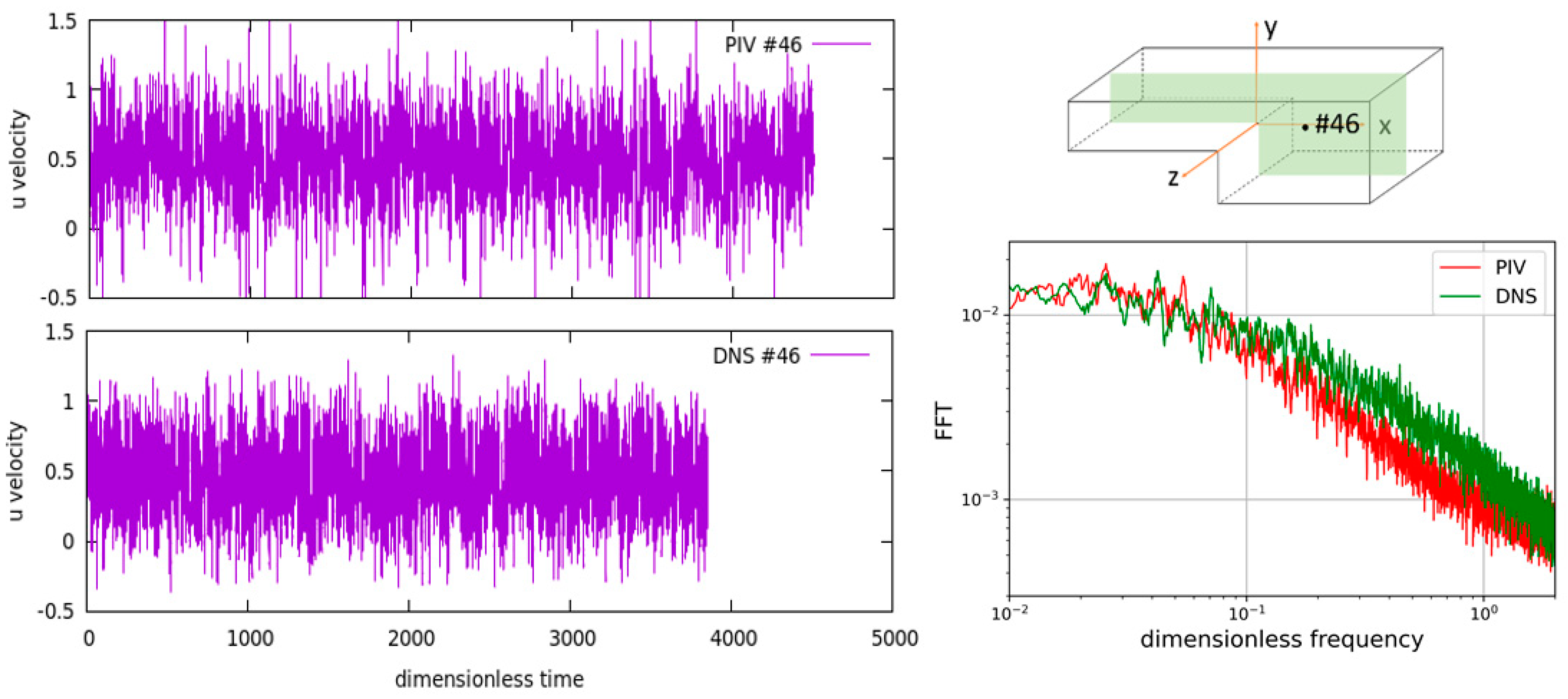
Figure 3 shows time histories of the streamwise velocity in a point at similar location in the PIV experiment and in the DNS. The point number #46 corresponds to the location #46 used in the uncertainty analysis of the DNS results performed by Oder et al. [32]. This analysis was based on time histories recorded in 50 points in the computational domain. The exact locations of the point #46 is slightly different in the experiment and DNS in order to get the data from a single spatial point without any spatial interpolation. Nevertheless, neighboring points in the experiment and DNS show similar qualitative behavior in the region, where turbulent kinetic energy of the flow is near its maximum.
The left graph of Figure 3 shows the frequency spectra of DNS and PIV at the point #46—similar behavior can be seen. It is important to note that a part of the DNS study [2,32] was also a quest for possible low frequency oscillations, which could point to the existence of the vortex shedding phenomena. However, such frequencies were not identified.
5. Results and Discussion
The results of the measurements, i.e., the velocities, velocity fluctuations and available components of Reynolds stress tensor, are discussed and compared with the DNS in four parts. Section 5.1 addresses the flow in the inlet section upstream of the step. Section 5.2 discusses the measurements of the recirculation zone taken in the planes z = const, where the most relevant properties of the recirculation can be identified. Section 5.3 discusses the measurements downstream the step in the planes y = const. that are, based on the DNS results of Oder et al. (2019), expected to be symmetric over the symmetry plane z = 0. Section 5.4 discusses profiles on line segments that lie at the intersections of the measurement planes y = const. and z = const. Lastly, Section 5.5 quantifies the uncertainties of the experiment.
5.1. Inlet Boundary Conditions
Comparison of the measurement and DNS starts in the inlet part of the test section. In the fully developed DNS, statistically steady turbulence is established through the implementation of the streamwise periodic boundary conditions on a short part (six dimensionless units) of the inlet section. In the experiments, fully developed flow is established with sufficiently long inlet section. The requirement for entrance length can be reduced if the large-scale turbulent structures are destroyed on the inlet. In the present test section, this was achieved with a diffusor: an acrylic piece covering the 20 mm × 45 mm2 cross-section entrance with 15 holes of 1 mm diameter distributed over the inlet surface. The preliminary analysis performed by Zajec et al. [28], according to the guidelines of White [34], resulted in the inlet part of the test section, which is 68 cm long (~25 hydraulic diameters).
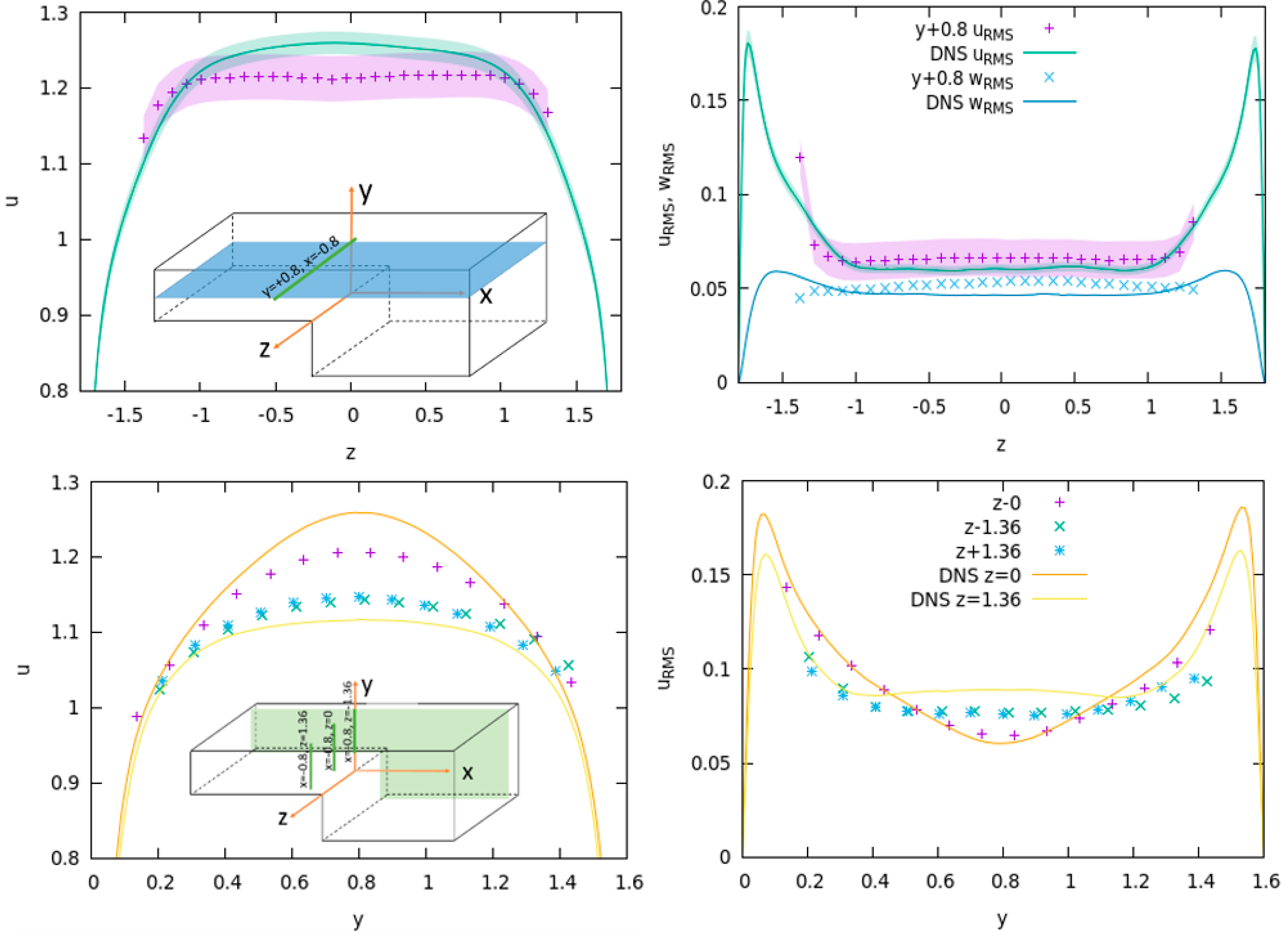
Inlet section streamwise velocity profiles and velocity RMS fluctuations are extracted from four measurements and compared with the DNS in Figure 4. All measurements and simulation results are taken 10 mm upstream of the step, which corresponds to x = −0.8 plane. Positions of the line segments where the profiles are taken are shown in the inset images. The two graphs at the top of Figure 4 show the u velocity and u and w velocity RMS fluctuation profiles extracted from the measurement case ‘y + 0.8’, while the bottom row of Figure 4 contains the profiles from the measurement cases ‘z − 1.36’, ‘z − 0’, and ‘z + 1.36’, together with two DNS profiles taken at x = −0.8, z = 0 and x = −0.8, z = +1.36. DNS profiles at x = −0.8, z = −1.36 are not given due to the symmetry of the z = −1.36 and z = +1.36 results.
Uncertainty bands in the top graphs of Figure 4 mark the magnitude of the measurement uncertainties in mean velocities and velocity fluctuations. Quantification of these uncertainties was performed a posteriori and is described in Section 5.5. A rough estimate is that the total measurement uncertainties are around two times larger than the statistical uncertainties of the measurements and DNS.
Several other observations follow from Figure 4:
- -
- Measured mean streamwise velocity profile is slightly flatter in the central region of the inlet section (Figure 4, top-left) than in the DNS. Maximum velocity in the axis of the inlet section DNS is higher than in the experiment, despite having the same Reynolds number and mass flow rate. On the other hand, measured mean velocities are higher near the walls (Figure 4, both left graphs: ~0.6 length units of the near-wall regions). We can see that uncertainty bands of both profiles overlap in most of the central region; however, the measurement and DNS seem to be consistent, and they both show very smooth profiles with clearly distinguishable difference. The same behavior is observed in the z direction and in y direction measurements. Thus, we believe that the flat measured profile, which is somewhat different than in the DNS, comes as a consequence of a slightly too short inlet section of around 25 hydraulic diameters based on the guidelines of [34]. In a recent review, most of the pipe entrance length studies analyzed by Düz [35] recommended 25–50 hydraulic diameters to achieve constant pressure gradient, but an even longer section, up to 100 hydraulic diameters, is needed to achieve fully developed values of the mean turbulent statistics, which are studied in the present paper. A longer inlet section gives more length and time for complete development of large-scale turbulent vortices [35]. Nevertheless, using the same argument, we cannot completely exclude the error on the side of DNS. There is a possibility that the periodic domain for the generation of inlet boundary conditions in DNS was too short and did not generate a sufficient amount of large-scale structures, despite being comparable with similar simulations in the literature.
- -
- Unlike in the DNS, the velocity profile in the experiment is weakly asymmetric in the z = 0 plane. Flow in the z > 0 half of the domain is slightly faster than in the z < 0 region. Weak asymmetry, which is visible in some measurement and is almost absent in other cases, is further shown in some of the figures below. The asymmetry was too weak to find the cause: the inlet diffusor has a symmetric arrangement of holes over the z = 0 plane and the dimensions of the test section were found to be accurate within the measurement accuracy of our length measuring tools.
- -
- Due to the proximity of the camera to the laser sheet plane (~20 cm), and the camera view that is centered on the details around x-axis, the near wall measurements are less accurate. Ideally, the walls of the section should be parallel to the line-of-sight; however, walls that are actually seen under the non-negligible angle and out-of-plane motions of particles might contribute to the error. Consequently, the boundary layers in the region of about 0.1 dimensionless units from the wall are poorly resolved in the measurements taken in z = const planes (bottom drawings of Figure 4). Due to the manufacturing method, unresolved near-wall layer is even larger in y = const. measurements (around 0.4 dimensionless length units). Since the focus of our study is not on the boundary layers but on the recirculation zone downstream the BFS, these non-accuracies in the near-wall regions were considered to be acceptable.
5.2. Recirculation Zone, Planes z = Const
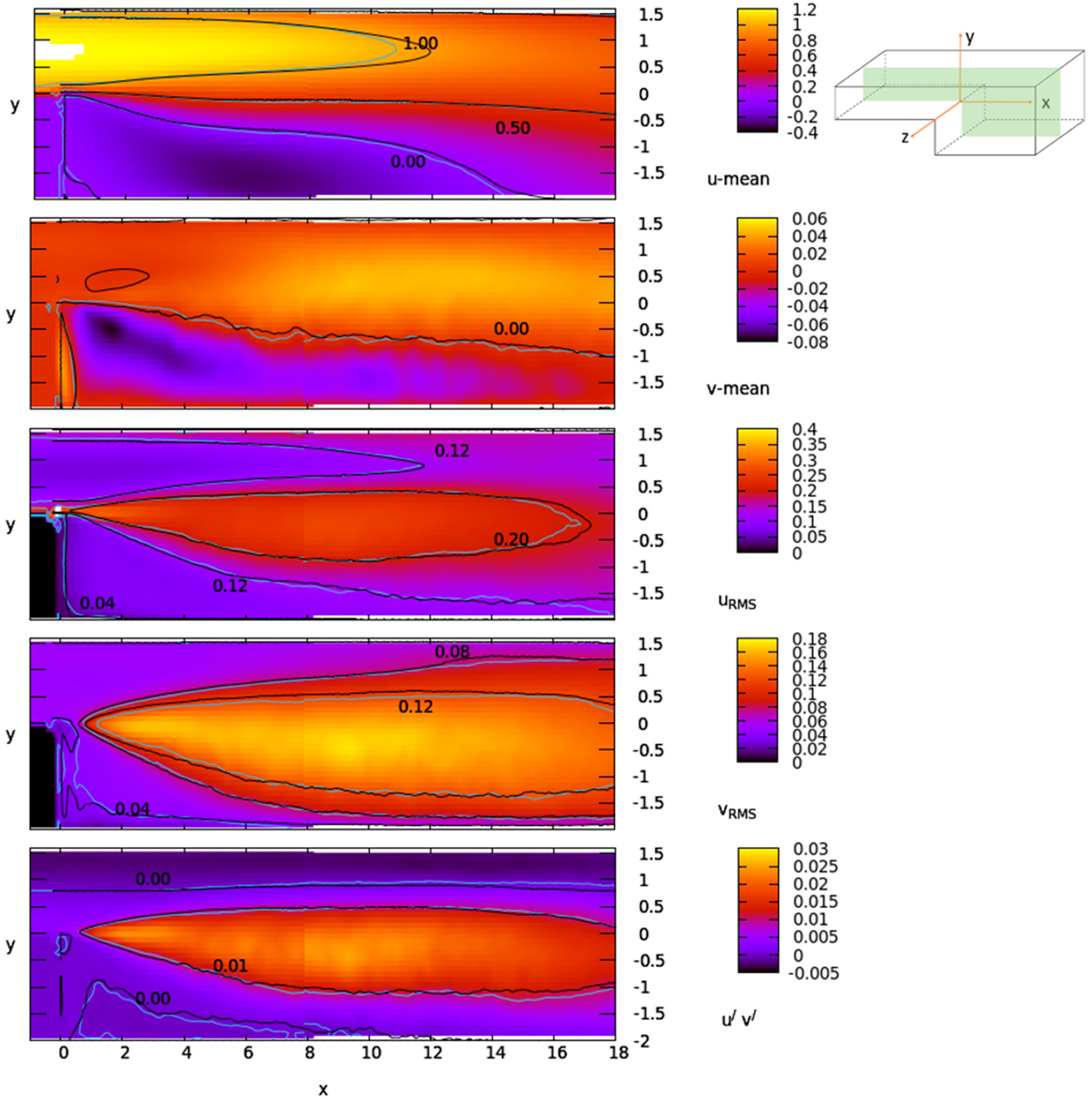
Figure 5 shows the 2D fields measured in the z = 0 plane; case ‘z − 0’ in Table 1. Case ‘z − 0’ consists of two separate measurements, which were merged in the post-processing phase.
Mild discontinuities can be observed in Figure 5 at x~8, where the fields are glued into a single image, and are a consequence of the uncertainties related to scaling of the images due to the uncertain laser and camera position. These systematic errors dominate the total uncertainty and are quantified for each measurement case in Section 5.5. Measurement data in each plane are available in two separate files, because the coordinates of the rows and columns in the global coordinate system of the experiment do not overlap.
The streamwise velocity field shown in Figure 5 shows the expected agreement of the measurements and the black simulation contours. A small vortex can be seen in the bottom left corner (x = 0 and y~−2) just downstream the step and is visible in both mean velocity components in Figure 5. The large vortex that spans down to the dimensionless length of x~15 (~20 cm behind the step) is clearly visible in the top image of Figure 5. Reattachment point at z = 0 is defined by the point where the contour 0.0 of u velocity touches the y = −2 plane. Due to the 3D nature of the flow, the reattachment point is actually not a point but a curve on the plane y = −2. The shape of the reattachment curve can be obtained from the measurements from the different perspective (y = const. planes), and is discussed in the next subsection. Several authors [1,18,19,20] reported that the size of the separation zone in separated flow depends not only on step height but also on the degree of turbulence in the upstream flow. In fact, it has been shown that the length of the separation region decreases with the increasing degree of turbulence in the upstream flow. In particular, Isomoto and Honami [19] measured the influence of turbulence on the length of the separation region behind the step with height of 40 mm at Reynolds number of 32,000. Our obtained reattachment point at the symmetry plane (i.e., plane z = 0) is 7.5 step heights downstream the step and it corresponds to the turbulence intensity of the inlet flow of about 4%. In general, the length of the separation region behind the step depends on the degree of expansion and asymmetry of the channel, and it varies from 6 to 9 calibers of the step height [1].
Bottom three images of Figure 5 show two components of the velocity fluctuations and one component of Reynolds stress tensor available from 2D measurement in z = 0 planes. One can see that the fluctuations created in the recirculation zone significantly exceed the fluctuations in the boundary layer of the inlet section: the maximum values of uRMS are almost two times higher and the maximum of vRMS is roughly three times higher.
The first consistency check, which also served as one of the measures of total uncertainty, was a check of the repeatability of the measurements, which was performed in the plane z = 0. Contours shown in Figure 6 compare the measurements of the ‘z − 0’ case and the case ‘z − 0a’, which was performed 10 days later under the same conditions. The expected agreement has demonstrated the repeatability of the measurements. Only contours of two parameters, u and vRMS, are shown in Figure 6, with the other three processed quantities showing a similar agreement. Dotted contours in Figure 6 show that positions of the violet contours increased and decreased for 0.03 and 0.01 for u and vRMS, respectively. These are values of the estimated uncertainty in the mean streamwise velocity and velocity fluctuations given in Section 5.5; however, they conveniently show the sensitivity of the measurements. DNS contours in Figure 6 are black and serve as an independent measure of the uncertainty.
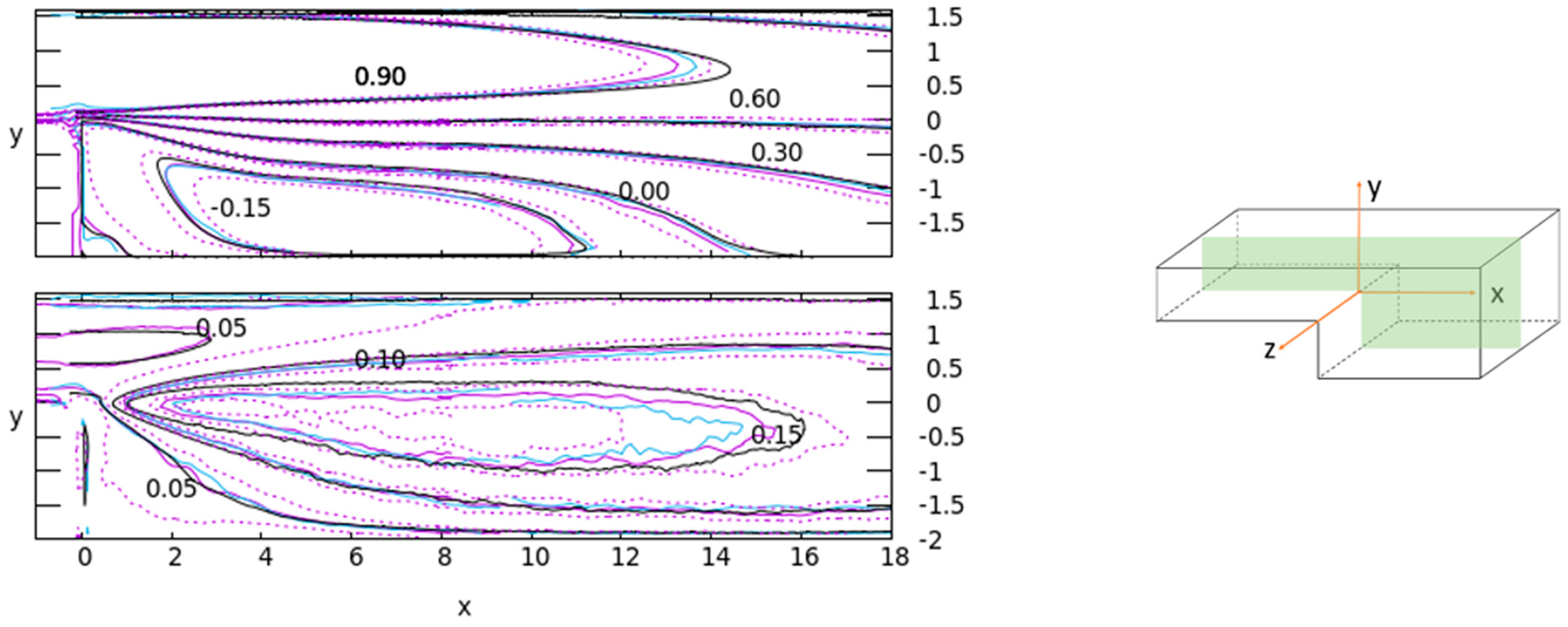
Beside carrying out the repeatability tests, we have also checked the consistency of our measurements against the flow symmetry in the z = 0 plane. Figure 7 compares two measurements taken in symmetry planes z = ±0.8 (‘z + 0.8’ and ‘z − 0.8’ cases) and two measurements taken in planes z = ±1.36 (‘z + 1.36’ and ‘z − 1.36’). Minor asymmetry of the flow, already observed in the inlet section flow, is seen here too: flow in the region z > 0 side (blue contours) of the domain is slightly faster than flow at z < 0 (violet contours). Especially the violet contour u = 0.0 of ‘z − 1.36’ seems to be far from the DNS and blue measurement. However, this contour is very sensitive to the laser sheet positioning error discussed in Section 4, as shown by the additional dotted contours that mark the experimental uncertainty band of each ‘z − 0’ contour.
Figure 7 shows another property mentioned in Section 5.1: the DNS velocity in the inlet section of the duct at y = 0.8 is higher than measurements at z~±0.8 and lower than the measured flow at z~±1.36.
A detailed comparison of the results from the contour plots and color fields is often too rough when one wants to verify the results of detailed computations and experiments. The profiles of the measured quantities at various line segments, such as the one shown in Figure 8, can provide a more accurate comparison. Three line segments in the plane z = 0 are selected, with their positions indicated in the sketch drawing in the top-right corner of Figure 8. The colors of the line segments in the sketch correspond to the colors of the lines used in graphs of Figure 8. Two solid lines in each graph correspond to the cases ‘z − 0’ and ‘z − 0a’ and were used as a part of the uncertainty analysis.
In Figure 8, better agreement of both measurements and DNS is observed for the first-order statistics, i.e., mean velocity components, and just slightly worse in the second-order statistics (velocity RMS fluctuations and Reynolds stress tensor component).
A single uncertainty bar is shown for each measurement in Figure 8. Evaluation of these uncertainties is described in Section 5.5. Similar graphs in other z = const. planes are not shown in the paper, but were created from the available database and used for uncertainty quantification. Agreement of DNS and measurement for the cases ‘z − 0.8’ and ‘z + 0.8’ is similar as in the ‘z − 0’ case. Slightly worse agreement was obtained for the cases ‘z − 1.36’ and ’z + 1.36’, which is mainly due to the rapid change of the recirculation vortex shape in the z direction, where even minor uncertainties in laser sheet position result in larger measurement errors.
5.3. Recirculation Zone, Planes y = Const
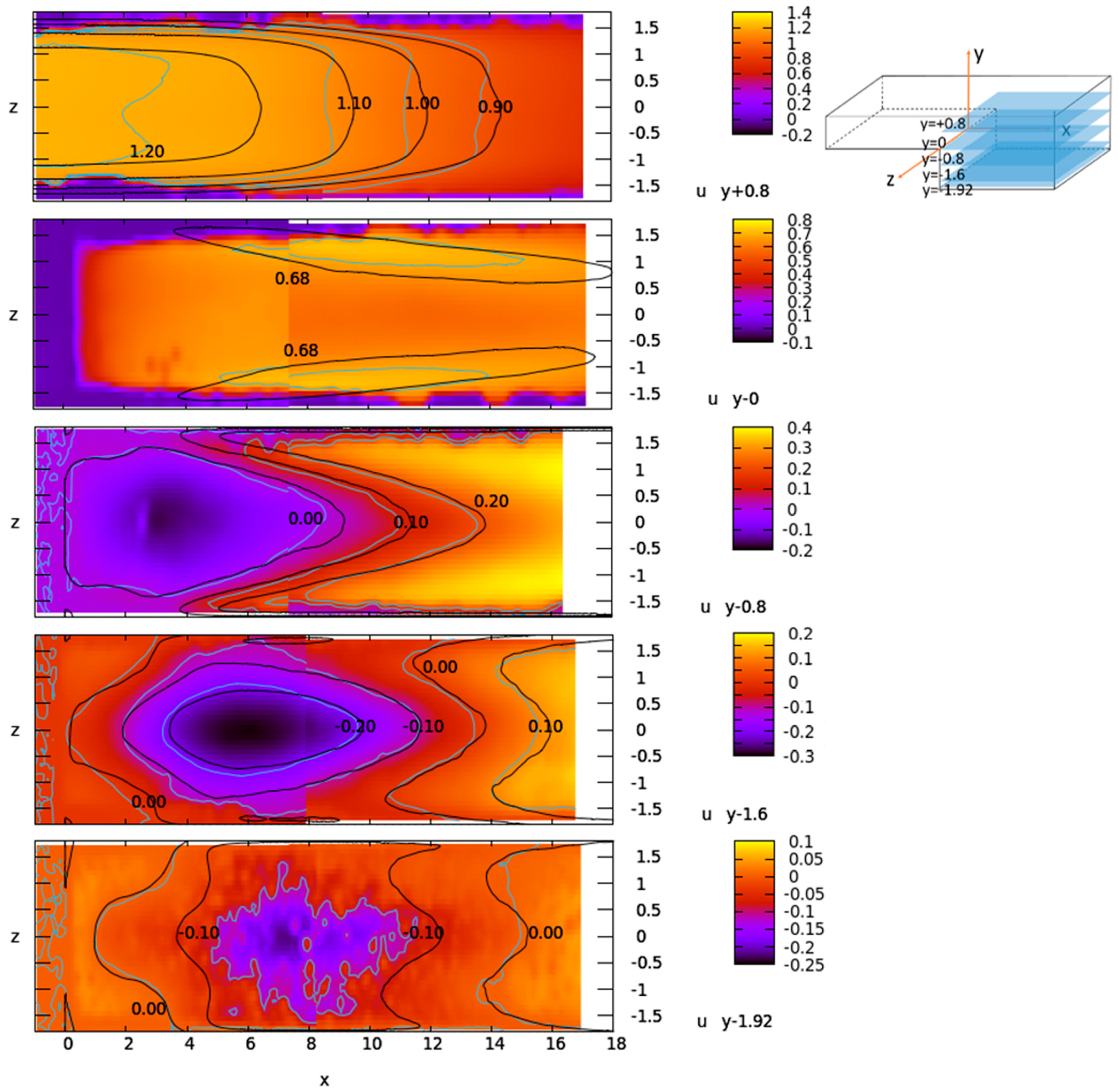
Results of the measurements in planes y = const. are shown in Figure 9 and Figure 10. Complete fields of streamwise velocity component u are shown in Figure 9, although, as already mentioned, the results in the near-wall regions of around 0.4 dimensionless units on each side should be ignored. Thus, the color fields and contours of the measurements at z > 1.4 and z < −1.4 should be disregarded in Figure 9. The profiles shown in Figure 10 have this part of the measurements already removed.
The top four measurements in Figure 9 at y = 0.8, 0, −0.8, −1.6 are made with comparable accuracy, while the bottom image in the plane y = −1.92 is close to the wall and less accurate. Plane position 1 mm away from the wall is in the region with large gradients and is consecutively very sensitive to laser sheet positioning. Thus, reasonable accuracy (quantification in Section 5.5) is available only for the first-order statistics, i.e., mean velocities.
Discontinuities in the merged images of each y = const. in Figure 9 are more pronounced than the discontinuities in the z = const. cases in Figure 5. This is expected because the flow field gradients in the y direction are larger than in the z direction. Consequently, measurements in y = const. planes are more sensitive to the uncertainties in the camera positions, scaling, and laser sheet position.
The y= −1.92 measurement shown in the bottom image of Figure 9 was performed in order to verify the length and the shape of the recirculation zone downstream the step. Despite the reduced accuracy of this measurement, taken 1 mm from the wall, with a laser sheet thickness of 1 mm, the results show good agreement with the recirculation zone length obtained in the DNS. Recirculation zone length is marked with u = 0.00 contour at a position of around x = 15.
The results in Figure 9 show another view on the slight asymmetry of the flow in the experiment, which was not observed in the DNS results. Despite the asymmetry, reasonable quantitative agreement with simulation is achieved. The seemingly large differences in the contours of the streamwise velocity u in Figure 9 are shown from a different aspect in Figure 10.
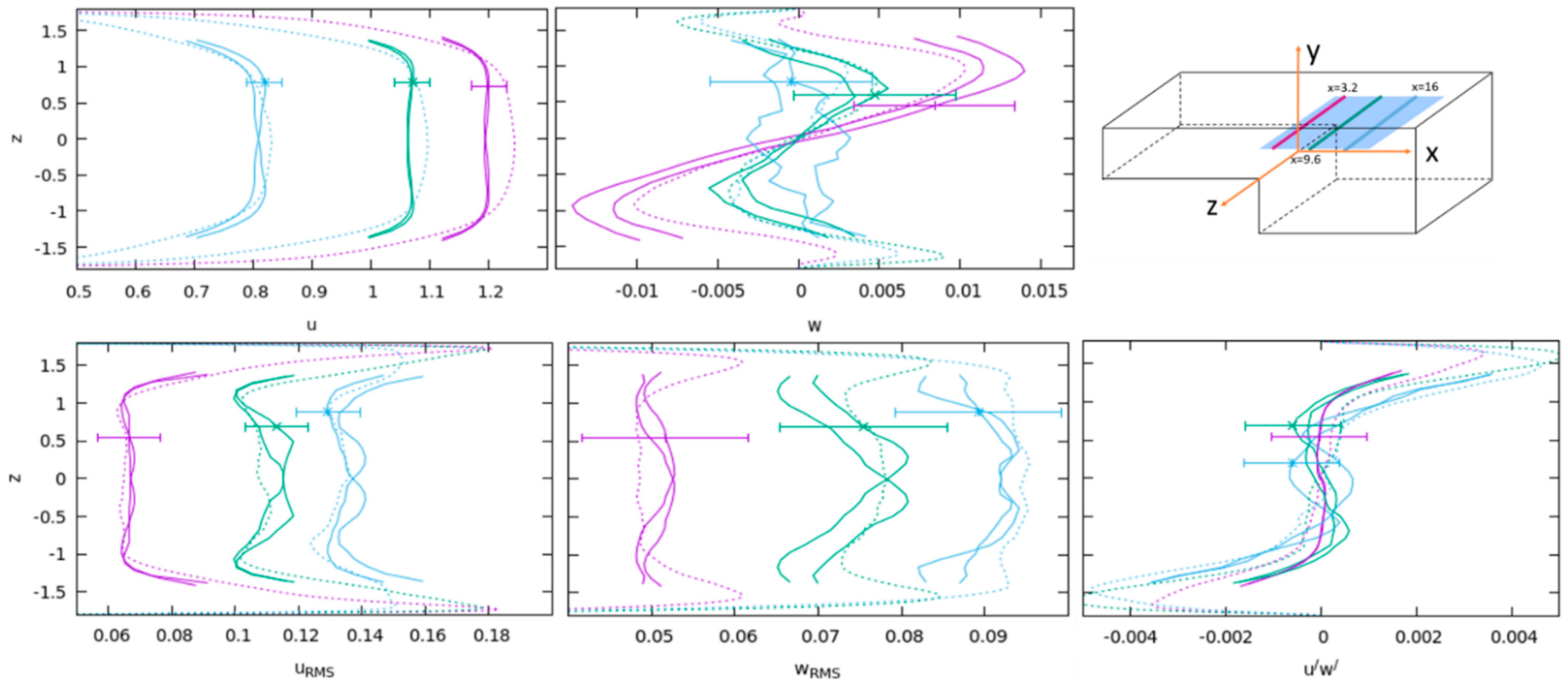
Figure 10 gives qualitative comparison of the measured and computed profiles of turbulence statistics in selected line segments on the y = 0.8 plane (case ‘y + 0.8’). Two solid curves on each graph are actually plots of the original measurement and the same measurement mirrored over the z = 0 plane. The symmetry of the measurements at z > 0 and z < 0 was used also to estimate the experimental uncertainty, which is plotted with a single uncertainty bar for each measurement and explained in Section 5.5.
Position of the line segments, where the profiles are plotted, is shown in the top-right sketch of Figure 10. Similar graphs with similar agreement can be obtained from the database at other y = const. planes, except the plane y = −1.92, where the accuracy of the measurements is deteriorated. Seemingly, larger differences are observed in the profiles of the w direction mean velocity; however, one should notice that the magnitudes of this velocity are very low: just around 1% of the mean flow velocity u and almost 10 times lower than the magnitude of the v velocity component shown in Figure 8. Agreement of the velocity RMS fluctuations is similar as the one observed in measurements in z = const. planes in Figure 8 and the agreement of the Reynolds stress component u′w′ is slightly worse than the one observed in Figure 8 for the component u′v′.
5.4. Results at the Cross-Section of the Planes z = Const and y = Const
The last check of consistency, used as another mean of uncertainty quantification of our measurements, was performed in the line segments that lie at the cross-sections of the measurement in planes z = const. and planes y = const. and were, thus, available from measurements taken from two different angles. Part of these results are shown in Figure 11, and others, which were also used for uncertainty quantification, can be extracted from the database.
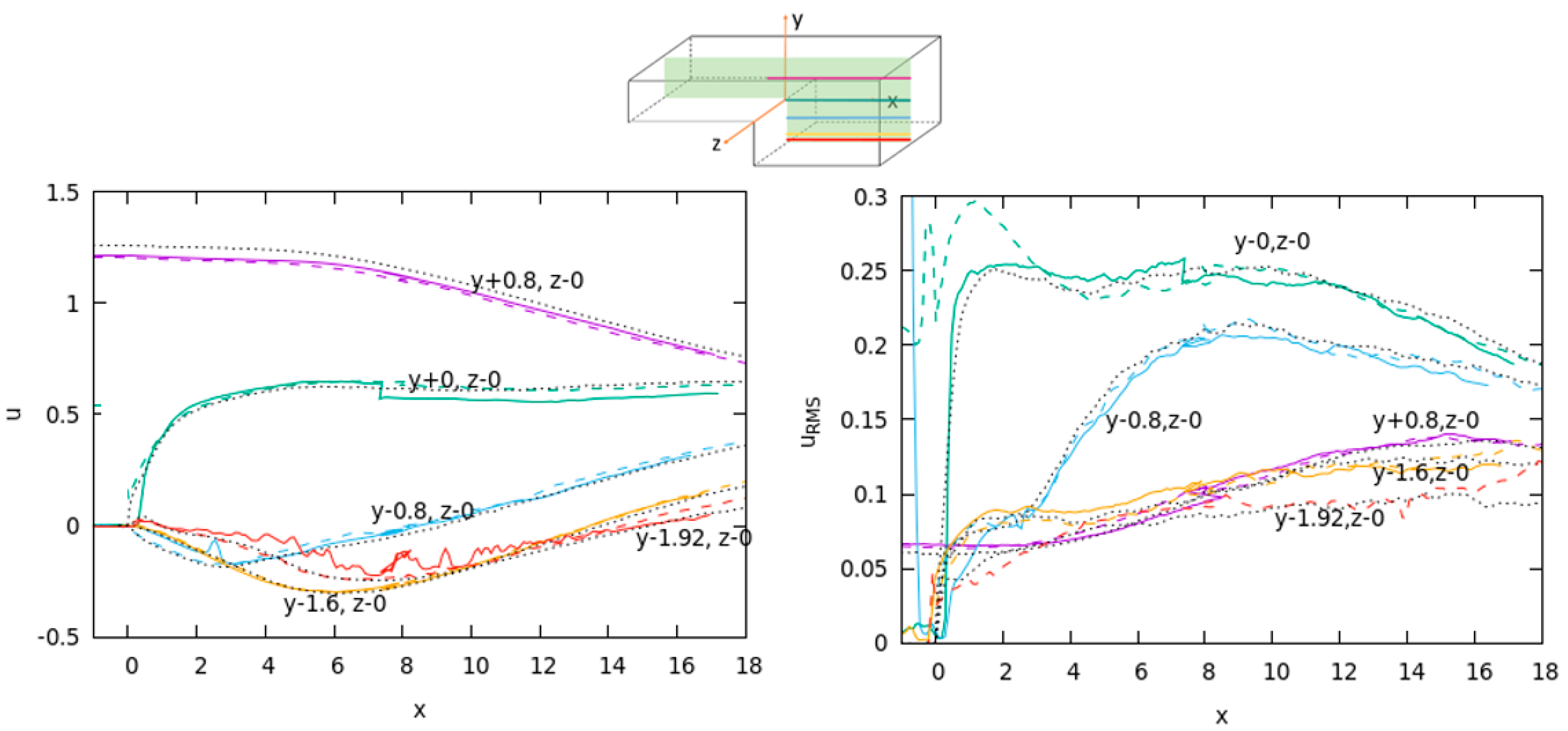
One must recall that the overall error of the measurements at ‘y − 0’ near the separation point is more susceptible to the accuracy of the laser sheet positioning as compared to other y = const. measurements due to high gradients at the contact of the recirculation zone and the main stream flow. Indeed, discontinuity of the merged fields in the mean u and uRMS is larger than in other cases. Higher uncertainties are observed also for the near-wall measurement ‘y − 1.92’, where only mean velocity u is show, while the uRMS exhibits fluctuations of around 0.04 dimensionless velocity units, which is not shown in the right graph.
Similar graphs to the one shown in Figure 11 were created at cross-sections of other four z = const planes and y = const planes and were used for uncertainty quantification.
The line segments at the cross-sections of z = const. and y = const. planes shown in Figure 11 are important for possible validation studies of CFD RANS turbulence models, since the measured profiles of the turbulence kinetic energy are available at these positions.
5.5. Uncertainties of the Measurements
Systematic and statistical uncertainties of the measurements were estimated together from all the available measurements. Total experimental uncertainties based on a review of a complete set of measurements are summarized in Table 2. They are expressed as absolute uncertainties and can be compared with orientation values: bulk velocity 1 and maximum uRMS fluctuations ~0.25. These integral uncertainties obtained from various properties of our measurements are based on the fact that we performed 22 independent (or weakly dependent) measurements, where 10 of them in y = const. planes exhibit an additional internal symmetry. Uncertainty quantification of each 2D measurement case was consequently performed on around 10 profiles of each particular variable taken at various streamwise or spanwise line segments on the 2D plane, and crosswise compared with results of other independent measurements of the same variable in the same line segments. As such, this set of independent measurements provides a reasonable estimate of the measurement uncertainties.
Different aspects of our measurements were used for quantification of uncertainties:
- -
- Repeatability of the measurement performed in plane z = 0 is discussed in Section 5.2. Next to the graphs shown for u and vRMS in Figure 6, graphs of other variables, v, uRMS and v’u’, were considered in the uncertainty analysis.
- -
- Comparison of the measurements in symmetry planes z = ±0.8 and z = ±1.36 is discussed in Section 5.2. Beside the comparison of the mean streamwise velocities shown in Figure 7, a symmetry check was also done for other variables. This comparison encompassed all measurement uncertainties, since the measurements in different z = const. planes are independent of each other; some of them were made on different days.
- -
- Quantification of the uncertainties in y = const. measurements were slightly less precise and were performed through mirroring of the measurements over the z = 0 plane, as shown in Figure 10 for plane y = 0.8. All other planes were analyzed in a similar fashion. The y = const. measurements do not encompass all systematic errors. Uncertainties due to the camera and laser sheet position are not available in a single measurement and only the discontinuities due to the merging of measurement pairs into a single dataset provided an insight into this type of uncertainties.
- -
- Measurements in z = const. and y = const. planes were analyzed in the line segments that represent intersections of these planes. This analysis gave us 25 line segments, where the streamwise velocity u and uRMS fluctuations can be compared from entirely independent measurements. An example of such analysis is discussed in Section 5.4 and in Figure 11 for 5 out of 25 available line segments. This approach allows more precise uncertainty quantification of u and uRMS, but not for other components of velocity and velocity fluctuations.
For orientation, we specify the uncertainties of the DNS, which are reported in Oder et al., 2019 and are due to statistical uncertainties of the time-averaging interval. The 2-sigma DNS uncertainties are 1–2% of the bulk velocity (1.5% or 0.015 dimensionless unit band is shown in the top-left Figure 4). Relative 2-sigma uncertainty of the second-order statistics (RMS fluctuations and Reynolds stress tensor components) is 4% (0.01 in dimensionless units) in the DNS (4% of maximal uRMS is used to plot uncertainty band of uRMS in DNS in Figure 4 top-right). The same statistical uncertainty applies to the experiment due to the similar length of the time-averaging interval; however, this uncertainty is added to the systematic errors, which are actually a dominant source of uncertainty in our experiment.
The overview of Table 2 shows that typical measurement uncertainties are up to two times larger than statistical uncertainties of the measurements and DNS. This estimate is applicable for recirculation zone, but not for the boundary layers, which are not covered in our measurements. Uncertainties closer to the walls (cases ‘z − 1.36’, ‘z + 1.36, ‘y − 1.92’) are larger than uncertainties in the central recirculation zone due to the higher near-wall gradients. A total of 2 out of 22 measurements, half of ‘y − 0’ and half of ‘y − 0.8’ case, were performed with a lower concentration of seeds and were, consequently, more uncertain. Good agreement of the measurements and the DNS result, which were not directly used for uncertainty quantification, confirms the quality of our database.
6. Conclusions
We have measured velocity field of water flowing over a confined backward-facing step with the 2D PIV system and compared the fields with the results of the DNS. Experiments and computations were performed at Reynolds number 7100. The measurements were performed in several planes from two different perspectives. The experiments presented in this paper were obtained after three years of training, gathering the experience with the PIV technique, gradual improvements of the test section, test loop, and camera and laser positioning techniques. The experiment has confirmed the predictions of the DNS about the flow behavior: shape of time-averaged vortices downstream the step, velocity fluctuations in the separation region, shape of the reattachment curve, and other properties. Comparison of PIV and DNS presents a mutual verification of both approaches.
Uncertainty of the velocity measurements was estimated by comparing different 1D profiles measured in different experimental cases on the same line segments. After the analysis of profiles in around 50 line segments of various orientations, the uncertainty of the streamwise velocity was estimated to be around 3–4% of the bulk velocity in the inlet section of the channel. This is roughly two times higher than in the DNS. The main contributions to the experimental uncertainty stem from the positioning of the camera and corresponding scaling of the results and from the laser sheet position.
We have shown that systematic uncertainty in laser sheet position results in negligible additional uncertainty when measurements are performed in the symmetry plane z = 0, while the same laser sheet position uncertainty becomes the dominant source of the total uncertainty, when measurements are performed closer to the walls, where gradients of the variables are large.
Improvement of the camera and laser sheet positioning to below 0.1 mm accuracy could produce measurements with accuracy comparable to the DNS, where the systematic measurement errors would be reduced below the statistical uncertainties of the finite time-averaging interval. When such an accuracy is reached, measurements (and DNS) should continue with much longer averaging times, if one would require results with further reduction of statistical uncertainties. In the specific case of the BFS flow at Reynolds number 7100, the required time-averaging interval should be increased from around 5 min to a few dozen minutes to reduce 2-sigma uncertainty of mean velocities below 1%.
Although the measurements are estimated to be slightly less accurate than DNS, they are accurate enough to raise some doubts about the sufficient entrance length of our experimental test section and of the DNS inlet flow boundary condition generator. Graphs in Figure 4 show small, but very consistent discrepancies of the measurement and simulation in the inlet part of the test section. Making a point-by-point wise comparison, both datasets are very close to each other’s uncertainty bands. However, the measurements (or simulation points) are not distributed randomly and show a very constant behavior over the recorded length interval. This difference could be a topic of our further experimental and numerical analyses.
Flow over the confined Backward-Facing Step is one of the simplest computationally and experimentally accessible geometries with the separation and reattachment of turbulent flows that can be used as a starting point for studies of the flows with sudden expansion. Such geometric changes are responsible for significant enhancement of turbulent mixing and heat and mass transfer. The measurements described in the present paper, combined with the existing DNS results by Oder et al. [2], represent a high-fidelity dataset, which can be used for benchmarking of the DNS computations and especially for the validation of other, less accurate LES and RANS turbulence models. Our preliminary results obtained with LES model on around 2.5 million mesh points, which has consumed more than two orders of magnitudes less CPU time than the DNS, show that the three-dimensional nature of the time-averaged flow makes the confined BFS flow a demanding validation case. While the LES results predict similar reattachment length as the PIV and the DNS in top image of Figure 5, the shape of the reattachment curve shown in the bottom image of Figure 9 shows differences, which will require further research of our LES models.
Author Contributions
B.Z.: development of the experimental loop, measurements of the three test sections; M.M.: development of the experimental loop, measurements of the first test section, paper review; N.K., measurement of the first and second test section, PIV processing, figures; J.O., DNS computation, DNS data processing; B.M., head of the lab, coordination and measurements of the second and third test section, paper review; J.K., measurements of the third test section; I.T., measurements of the second and third test section, PIV processing, writing. All authors have read and agreed to the published version of the manuscript.
Funding
This research was funded by the Slovenian Research Agency, grants P2-0026 and L2-9210. and SESAME project funded by the EURATOM Research and Training Programme (#654935) of the European Commission (H2020).
Institutional Review Board Statement
Not applicable.
Informed Consent Statement
Not applicable.
Data Availability Statement
Experimental and DNS databases of the confined BFS flow are in open access. Contact: Jure Oder (DNS) and Iztok Tiselj (PIV).
Acknowledgments
The authors acknowledge the financial support of the Slovenian Research Agency and Nuklearna Elektrarna Krško for the project L2-9210, and of the Slovenian Research Agency research core funding No. P2-0026.
Conflicts of Interest
The authors declare no conflict of interest.
References
- Terekhov, V.I. Heat Transfer in Highly Turbulent Separated Flows: A Review. Energies 2021, 14, 1005. [Google Scholar] [CrossRef]
- Oder, J.; Shams, A.; Cizelj, L.; Tiselj, I. Direct numerical simulation of low-Prandtl fluid flow over a confined backward facing step. Int. J. Heat Mass Transfer. 2019, 142, 118436. [Google Scholar] [CrossRef]
- Da Vià, R.; Giovacchini, V.; Manservisi, S. A Logarithmic Turbulent Heat Transfer Model in Applications with Liquid Metals for Pr = 0.01–0.025. Appl. Sci. 2020, 10, 4337. [Google Scholar] [CrossRef]
- Schaub, T.; Arbeiter, F.; Hering, W.; Stieglitz, R. Forced and mixed convection experiments in a confined vertical backward facing step at low-Prandtl number, to appear in Exp. Fluids 2021. [Google Scholar] [CrossRef]
- Kim, J.; Kline, S.J.; Johnston, J.P. Investigation of a reattaching turbulent shear layer: Flow over a backward-facing step. J. Fluids Eng. 1980, 102, 302. [Google Scholar] [CrossRef]
- Abbott, D.E.; Kline, S.J. Experimental investigation of subsonic turbulent flow over single and double backward facing steps. J. Basic Eng. 1962, 84, 317. [Google Scholar] [CrossRef]
- De Brederode, V.; Bradshaw, P. Three-Dimensional Flow in Nominally Two Dimensional Separation Bubbles. I, Flow behind a Rearward-Facing Step; I.C. Aero Report 1972; Department of Aeronautics, Imperial College of Science and Technology: London, UK, 1972. [Google Scholar]
- Armaly, B.F.; Durst, F.; Pereira, J.C.F.; Schönung, B. Experimental and theoretical investigation of backward-facing step flow. J. Fluid Mech. 1988, 127, 473–496. [Google Scholar] [CrossRef]
- Kasagi, N.; Matsunaga, A. Three-dimensional particle-tracking velocimetry measurement of turbulence statistics and energy budget in a backward-facing step flow. Int. J. Heat Fluid Flow 1995, 16, 477–485. [Google Scholar] [CrossRef]
- Beaudoin, J.-F.; Cadot, O.; Aider, J.-L.; Wesfreid, J.E. Three-dimensional stationary flow over a backward-facing step. Eur. J. Mech.—B/Fluids 2004, 23, 147–155. [Google Scholar] [CrossRef] [Green Version]
- Liakos, A.; Malamataris, N.A. Topological study of steady state, three dimensional flow over a backward facing step. Comput. Fluids 2015, 118, 1–18. [Google Scholar] [CrossRef]
- Buckingham, S. Prandtl Number Effects in Abruptly Separated Flows: LES and Experiments on an Unconfined Backward Facing Step. Ph.D. Thesis, Université Catholique de Louvain, Ottignies-Louvain-la-Neuve, Belgium, 2018. [Google Scholar]
- Chen, L.; Asai, K.; Nonomura, T.; Xi, G.; Liu, T. A review of backward-facing step (BFS) flow mechanisms, heat transfer and control. Thermal Sci. Eng. Prog. 2018, 6, 194–216. [Google Scholar] [CrossRef]
- Polewski, M.D.; Cizmas, P.G.A. Several Cases for the Validation of Turbulence Models Implementation. Appl. Sci. 2021, 11, 3377. [Google Scholar] [CrossRef]
- Pont-Vílchez, A.; Trias, F.; Gorobets, A.; Oliva, A. Direct numerical simulation of backward-facing step flow at and expansion ratio 2. J. Fluid Mech. 2019, 863, 341–363. [Google Scholar] [CrossRef] [Green Version]
- Schumm, T.; Frohnapfel, B.; Marocco, L. Investigation of a turbulent convective buoyant flow of sodium over a backward-facing step flow. Heat Mass Transf. 2018, 54, 2533–2543. [Google Scholar] [CrossRef]
- Oder, J.; Tiselj, I.; Jaeger, W.; Schaub, T.; Hering, W.; Otic, I.; Shams, A. Thermal fluctuations in low-Prandtl number fluid flows over a backward facing step. Nucl. Eng. Des. 2020, 359, 110460. [Google Scholar] [CrossRef]
- Terekhov, V.I.; Yarygina, N.I.; Zhdanov, R.F. Heat transfer in turbulent separated flows in the presence of high free-stream turbulence. Int. J. Heat Mass Transf. 2003, 46, 4535–4551. [Google Scholar] [CrossRef]
- Isomoto, K.; Honami, S. The effect of inlet turbulence intensity on the reattachment process over a backward-facing step. JSME 1988, B54, 51–58. [Google Scholar] [CrossRef] [Green Version]
- Jaňour, Z.; Jonás, P. On the flow in a channel with a backward-facing step on one wall. Eng. Mech. 1994, 1, 313–320. [Google Scholar]
- Wang, F.; Gao, A.; Wu, S.; Zhu, S.; Dai, J.; Liao, Q. Experimental Investigation of Coherent Vortex Structures in a Backward-Facing Step Flow. Water 2019, 11, 2629. [Google Scholar] [CrossRef] [Green Version]
- Le, H.; Moin, P.; Kim, J. Direct numerical simulation of turbulent flow over a backward-facing step. J. Fluid Mech. 1997, 330, 349–374. [Google Scholar] [CrossRef] [Green Version]
- Zhao, P.; Wang, C.; Ge, Z.; Zhu, J.; Liu, J.; Ye, M. DNS of turbulent mixed convection over a vertical backward-facing step for lead-bismuth eutectic. Int. J. Heat Mass Transf. 2018, 127, 1215–1229. [Google Scholar] [CrossRef]
- Lim, K.S.; Park, S.O.; Shim, H.S. A low aspect ratio backward-facing step flow. Exp. Therm. Fluid Sci. 1990, 3, 508–514. [Google Scholar] [CrossRef]
- Nie, J.H.; Armaly, B.F. Reverse flow regions in three-dimensional backward-facing step flow. Int. J. Heat Mass Transf. 2004, 47, 4713–4720. [Google Scholar] [CrossRef]
- Piirto, M.; Karvinen, A.; Ahlstedt, H.; Saarenrinne, P.; Karvinen, R. PIV Measurements in Square Backward-Facing Step. J. Fluids Eng. ASME 2007, 129, 984–990. [Google Scholar] [CrossRef]
- Barri, M.; El Khoury, G.K.; Andersson, H.I.; Pettersen, B. DNS of backward-facing step flow with fully turbulent inflow. Int. J. Numer. Meth. Fluids 2010, 64, 777–792. [Google Scholar] [CrossRef] [Green Version]
- Zajec, B.; Oder, J.; Matkovič, M. Two-dimensional PIV Measurements of Water Flow Over a Backward-facing Step. In Proceedings of the NENE 2018, 27th Conference Nuclear Energy for New Europe, Portorož, Slovenia, 10–13 September 2018. [Google Scholar]
- Argyropoulos, C.D.; Markatos, N.C. Recent advances on the numerical modelling of turbulent flows. Appl. Math. Model. 2015, 39, 693–732. [Google Scholar] [CrossRef]
- Weaver, D.; Miškovic, S. A Study of RANS Turbulence Models in Fully Turbulent Jets: A Perspective for CFD-DEM Simulations. Fluids 2021, 6, 271. [Google Scholar] [CrossRef]
- Fisher, P.F.; Lottes, J.W.; Kerkemeier, S.G. nek5000 Web Page. Available online: http://nek5000.mcs.anl.gov (accessed on 15 June 2021).
- Oder, J.; Flageul, C.; Tiselj, I. Statistical Uncertainty of DNS in Geometries without Homogeneous Directions. Appl. Sci. 2021, 11, 1399. [Google Scholar] [CrossRef]
- Sciacchitano, A. Uncertainty quantification in particle image velocimetry. Meas. Sci. Technol. 2019, 30, 092001. [Google Scholar] [CrossRef] [Green Version]
- White, F.M. Fluid Mechanics, 7th ed.; McGraw-Hill Education Ltd.: New York, NY, USA, 2011. [Google Scholar]
- Düz, H. Numerical and experimental study to predict the entrance length in pipe flows. J. Appl. Fluid Mech. 2019, 12, 155–164. [Google Scholar] [CrossRef]
Figure 1.
Left: Test loop configuration. Top-right: Schematic of the test-section, coordinate system and measurement planes z = 0 (green) and y = 0 (blue). In parentheses: dimensionless lengths. X-length of the measurement planes is around 25 cm. Bottom-right: raw image for PIV analysis in plane z = 0.

Figure 2.
Top: DNS spectral element mesh. Bottom: reference mesh dimension divided by the local Kolmogorov scale in the z = 0 plane.
Figure 2.
Top: DNS spectral element mesh. Bottom: reference mesh dimension divided by the local Kolmogorov scale in the z = 0 plane.

Figure 3.
Time history of the streamwise velocity component u in point #46. PIV: (5.83, −0.16, 0), DNS: (6, −0.2, 0). Top-left: experiment, case ‘z − 0’, Bottom-left: DNS. Bottom-right: frequency spectra of PIV and DNS time histories in point #46.
Figure 3.
Time history of the streamwise velocity component u in point #46. PIV: (5.83, −0.16, 0), DNS: (6, −0.2, 0). Top-left: experiment, case ‘z − 0’, Bottom-left: DNS. Bottom-right: frequency spectra of PIV and DNS time histories in point #46.

Figure 4.
Top: profiles of u (left), uRMS, wRMS (right) at line segment x = −0.8, case ‘y + 0.8’ in Table 1 (green line on top inset drawing). Bottom: profiles of u (left), uRMS (right) at line segments x = −0.8 in cases ‘z − 0’, ‘z − 1.36’, ‘z + 1.36’ (green lines on bottom inset drawing). Symbols: PIV, lines: DNS.

Figure 5.
Time-averaged velocity field of case ‘z − 0’: components u and v (top pair), uRMS,vRMS, u’v’ (bottom triplet) in plane z = 0. PIV experiment: color-scale and blue contours. DNS—black contours.
Figure 5.
Time-averaged velocity field of case ‘z − 0’: components u and v (top pair), uRMS,vRMS, u’v’ (bottom triplet) in plane z = 0. PIV experiment: color-scale and blue contours. DNS—black contours.

Figure 6.
Streamwise velocity u contours (top) and vRMS (bottom) in plane z = 0. Solid contours: case ‘z − 0’—violet, case ‘z − 0a’—blue, DNS—black. Violet dotted contours: sensitivity contours of ‘z − 0’ case; ±0.03 and ±0.01 for u and vRMS, respectively.
Figure 6.
Streamwise velocity u contours (top) and vRMS (bottom) in plane z = 0. Solid contours: case ‘z − 0’—violet, case ‘z − 0a’—blue, DNS—black. Violet dotted contours: sensitivity contours of ‘z − 0’ case; ±0.03 and ±0.01 for u and vRMS, respectively.

Figure 7.
Flow symmetry: time-averaged u velocity contours. Top: measurements ‘z − 0.8’ (violet) and ‘z + 0.8’ (blue). Bottom: measurements ‘z − 1.36’ (violet), ‘z + 1.36’ (blue). DNS—black contours. Dotted violet contours: sensitivity contours at ±0.03 units of ‘z − 0.8’ (top) and ‘z − 1.36’ (bottom) cases.

Figure 8.
Measurements ‘z − 0’ and ‘z − 0a’. Profiles at x = 3.2, 9.6, 16 mm. Variables: u, v, uRMS, vRMS, and u′v′. Measurements—solid lines. DNS—dotted lines. Uncertainties are given for ‘z − 0’ measurement in a single point per profile.
Figure 8.
Measurements ‘z − 0’ and ‘z − 0a’. Profiles at x = 3.2, 9.6, 16 mm. Variables: u, v, uRMS, vRMS, and u′v′. Measurements—solid lines. DNS—dotted lines. Uncertainties are given for ‘z − 0’ measurement in a single point per profile.

Figure 9.
Time-averaged field of velocity component u in all y = const. planes. Measurements—color scale and blue contours. DNS—black contours.
Figure 9.
Time-averaged field of velocity component u in all y = const. planes. Measurements—color scale and blue contours. DNS—black contours.

Figure 10.
Measurement ‘y + 0.8’, profiles at x = 3.2, 9.6, 16. Variables: u, w, uRMS, wRMS, and u′w′. Solid lines: original measurements and measurements mirrored over z = 0. DNS—dotted lines. Uncertainties are given in a single point per profile.
Figure 10.
Measurement ‘y + 0.8’, profiles at x = 3.2, 9.6, 16. Variables: u, w, uRMS, wRMS, and u′w′. Solid lines: original measurements and measurements mirrored over z = 0. DNS—dotted lines. Uncertainties are given in a single point per profile.

Figure 11.
Mean streamwise velocity u and velocity fluctuations uRMS at cross-sections of the measurement planes. Dashed lines: profiles of the case ‘z − 0’ in line segments at y = −1.92, −1.6, −0.8, 0, 0.8. Solid lines: profiles from cases ‘y − 1.92’, ‘y − 1.6’, ‘y − 0.8’, ‘y − 0’, and ‘y + 0.8’ at z = 0. DNS—black dotted lines.


Table 1.
List of measurements in the planes z = const. and in the planes y = const. Each case contains two measurements: one with camera at position at x = 4 cm and another at x = 16 cm. Reynolds numbers are given for each of them.
Table 1.
List of measurements in the planes z = const. and in the planes y = const. Each case contains two measurements: one with camera at position at x = 4 cm and another at x = 16 cm. Reynolds numbers are given for each of them.
| Case Name | Re | z (mm) | z Dimensionless |
|---|---|---|---|
| ‘z − 1.36’ | 7120, 7120 | −17 | −1.36 |
| ‘z − 0.8’ | 7140, 7120 | −10 | −0.8 |
| ‘z − 0’ | 7120, 7120 | 0 | 0 |
| ‘z + 0.8’ | 7120, 7120 | 10 | 0.8 |
| ‘z + 1.36’ | 7120, 7120 | 17 | 1.36 |
| ‘z − 0a’ | 7130, 7120 | 0 | 0 |
| y (mm) | y Dimensionless | ||
| ‘y + 0.8’ | 7120, 7120 | 10 | 0.8 |
| ‘y − 0’ | 7120, 7120 | 0 | 0 |
| ‘y − 0.8’ | 7130, 7130 | −10 | −0.8 |
| ‘y − 1.6’ | 7110, 7130 | −20 | −1.6 |
| ‘y − 1.92’ | 7130, 7120 | −24 | −1.92 |
Table 2.
Absolute uncertainties of measured quantities rounded to the leading digit (* uncertainties up to 0.05 are present in the interval 0 < x < 3 where maximum uRMS values are measured and calculated).
Table 2.
Absolute uncertainties of measured quantities rounded to the leading digit (* uncertainties up to 0.05 are present in the interval 0 < x < 3 where maximum uRMS values are measured and calculated).
| Case Name | u | uRMS | v | vRMS | u’v’ |
|---|---|---|---|---|---|
| ‘z − 1.36’ | 0.03 | 0.02 * | 0.02 | 0.01 | 0.003 |
| ‘z − 0.8’ | 0.03 | 0.01 * | 0.01 | 0.01 | 0.003 |
| ‘z − 0’ | 0.03 | 0.01 * | 0.007 | 0.01 | 0.003 |
| ‘z + 0.8’ | 0.03 | 0.01 * | 0.01 | 0.01 | 0.003 |
| ‘z + 1.36’ | 0.03 | 0.02 * | 0.02 | 0.01 | 0.003 |
| ‘z − 0a’ | 0.03 | 0.01 * | 0.007 | 0.01 | 0.003 |
| u | uRMS | w | wRMS | u’w’ | |
| ‘y + 0.8’ | 0.03 | 0.01 | 0.005 | 0.01 | 0.001 |
| ‘y − 0’ | x < 8: 0.15 x > 8: 0.03 | x < 8: 0.04 x > 8: 0.01 | 0.007 | 0.02 | 0.002 |
| ‘y − 0.8’ | x < 8: 0.05 x > 8: 0.03 | x < 8: 0.02 x > 8: 0.01 | 0.01 | 0.01 | 0.004 |
| ‘y − 1.6’ | 0.03 | 0.01 | 0.02 | 0.01 | 0.002 |
| ‘y − 1.92’ | 0.08 | 0.04 | / | / | / |
Publisher’s Note: MDPI stays neutral with regard to jurisdictional claims in published maps and institutional affiliations. |
© 2021 by the authors. Licensee MDPI, Basel, Switzerland. This article is an open access article distributed under the terms and conditions of the Creative Commons Attribution (CC BY) license (https://creativecommons.org/licenses/by/4.0/).
Share and Cite
MDPI and ACS Style
Zajec, B.; Matkovič, M.; Kosanič, N.; Oder, J.; Mikuž, B.; Kren, J.; Tiselj, I. Turbulent Flow over Confined Backward-Facing Step: PIV vs. DNS. Appl. Sci. 2021, 11, 10582. https://doi.org/10.3390/app112210582
AMA Style
Zajec B, Matkovič M, Kosanič N, Oder J, Mikuž B, Kren J, Tiselj I. Turbulent Flow over Confined Backward-Facing Step: PIV vs. DNS. Applied Sciences. 2021; 11(22):10582. https://doi.org/10.3390/app112210582
Chicago/Turabian StyleZajec, Boštjan, Marko Matkovič, Nejc Kosanič, Jure Oder, Blaž Mikuž, Jan Kren, and Iztok Tiselj. 2021. "Turbulent Flow over Confined Backward-Facing Step: PIV vs. DNS" Applied Sciences 11, no. 22: 10582. https://doi.org/10.3390/app112210582
Note that from the first issue of 2016, this journal uses article numbers instead of page numbers. See further details here.