A Logarithmic Turbulent Heat Transfer Model in Applications with Liquid Metals for Pr = 0.01–0.025

Abstract

The study of turbulent heat transfer in liquid metal flows has gained interest because of applications in several industrial fields. The common assumption of similarity between the dynamical and thermal turbulence, namely, the Reynolds analogy, has been proven to be invalid for these fluids. Many methods have been proposed in order to overcome the difficulties encountered in a proper definition of the turbulent heat flux, such as global or local correlations for the turbulent Prandtl number and four parameter turbulence models. In this work we assess a four parameter logarithmic turbulence model for liquid metals based on the Reynolds Averaged Navier-Stokes (RAN) approach. Several simulation results considering fluids with $Pr=0.01$ and $Pr=0.025$ are reported in order to show the validity of this approach. The Kays turbulence model is also assessed and compared with integral heat transfer correlations for a wide range of Peclet numbers.

1. Introduction

The fluid-dynamics of low-Prandtl-number liquid metals is currently being studied due to an increasing interest in the applications of these fluids in engineering problems. Advanced nuclear reactor designs cooled with liquid metals have been proposed in the Generation IV Forum and some liquid metal fast nuclear reactors have been built and operated [1]. Liquid metal fluid dynamics is also studied in other engineering fields as they are considered possible coolants for new solar power systems [2]. These fluids show low dynamical viscosity with high thermal conductivity and therefore low Prandtl numbers. Two main important coolants for Generation IV nuclear reactors are sodium and lead–bismuth eutectic. The coolant Prandtl number depends on the operational temperature of the reactor; in particular, with increasing temperature the Prandtl number decreases. The Prandtl number of lead–bismuth eutectic is in the range of $0.03$–$0.01$, while sodium has a lower Prandtl with values ranging from $0.01$ to $0.005$ [3]. Despite the increasing interest in reliable computational tools for these fluids for the study of turbulent heat transfer in complex industrial applications with liquid metals, they are still lacking in commercial codes.

The study of reliable and robust computational techniques to deal with this problem is still in the development phase [1,4,5,6,7,8]. Due to the complexity of the modeling, different approaches have been proposed by different authors. Grötzbach in his work [1] attempted to model the temperature variance equation for turbulent natural convection; meanwhile, Cheng et al. in [4] proposed a modeling of the turbulence Prandtl number based on experimental data in circular tubes. Near-wall modeling and Kays correlation based on Large Eddy Simulations (LES) for forced convection at low Prandtl numbers is described by Duponcheel et al. [5] and Bricteux et al. in [6]. Shams et al. in [7] presented an overview of different algebraic models for prediction of heat transfer turbulent flow. In Manservisi et al. [8] a four equation turbulence model is introduced for single rod and rod bundle simulations.

Direct numerical simulations are being used to investigate these physical phenomena but an accurate prediction of heat transfer in industrial applications, such as heat exchangers or nuclear reactor pools, cannot rely on this technique due to limitations of the available computational resources [6,9,10,11,12]. On the other hand, numerical data obtained with Direct Numerical Simulations (DNS) are of strong interest for the validation of turbulence models based on Reynolds averaging Navier–Stokes approach because they can be used to finely tune the turbulence model in the low-Reynolds-number regime. Reynolds Averaged Navier-Stokes (RANS) modeling has been successfully employed in multiple sectors, such as aeronautical, the automotive industry, the nuclear industry and many other fields where DNS is not affordable. In this framework it is very common to assume similarity between the dynamical and thermal turbulent transfer and therefore to define a constant, turbulent Prandtl number as the ratio between the eddy viscosity and eddy thermal diffusivity. For fluids with $Pr$ ∼ 1 the turbulent Prandtl number is set to $P{r}_t$ = 0.85–0.9, but for liquid-metal flows this assumption is known to be invalid [4,5,7].

Several solutions have been proposed to deal with this problem. One possible method is to evaluate the turbulent Prandtl number by means of correlations employing global parameters of the flow, such as Reynolds or Peclet numbers. In Cheng et al. [4] a constant $P{r}_t$ is assumed on the whole domain, case by case, as a function of the Reynolds number. Another possible solution is to define a local turbulent Prandtl number as a function of flow variables, as proposed by Kays [13]. In their work, Duponcheel et al. [5] studied this and other local or global correlations and compared the results obtained in a few test cases. They concluded that Kays correlation is the most reliable one among existing local correlations for RANS computations. The key point in many of these approaches is that the correlation has to be defined and validated for each geometry. Another different approach is to define the turbulent heat diffusivity with specific time scales resolved by the introduction of the dissipation rate of both temperature and velocity fluctuations. These models have been studied by some authors for forced convection and buoyant flows in different geometrical configurations [7,8,14,15]. The effects of geometries with injection and suction at the wall are simulated in [14,15] with a two-equation turbulent thermal model. In Shams et al. [7] an overview of different realistic geometries for liquid-metal applications in the field of nuclear engineering is summarized with the help of several Computational Fluid Dynamic (CFD) models and tools. A four-parameter turbulence model k-$\epsilon$-$k_{\theta }$-${\epsilon }_{\theta }$, based on Abe and Nagano’s model [15,16,17,18], was introduced by Manservisi and Menghini [8]. The model has been validated against DNS and experimental correlation data, with simulations of $Pr=0.025$ fluids for several geometries, involving plane channels, cylindrical ducts and triangle and square bundle lattices [8,19,20]. With the purpose of improving the numerical stability of the model, a change of state variables has been considered in [21], where specific dissipation rates $\omega$ and ${\omega }_{\theta }$ have been used in place of $\epsilon$ and ${\epsilon }_{\theta }$, and in [22], where, by following the work of [23], logarithmic values of $\omega$ and ${\omega }_{\theta }$, i.e., $\mathsf{\Omega }$ and ${\mathsf{\Omega }}_{\theta }$, have been used. As a consequence of the change of state variables, some model coefficients had to be changed in order to improve the numerical stability, and the resulting models have been validated with simulations of plane channels and cylindrical ducts for $Pr=0.025$. The model, in a fully logarithmic version and with additional terms accounting for buoyancy, has also been used to simulate a sodium turbulent flow over a backward facing step geometry, with $Pr=0.0088$, in the cases of forced and mixed convection [24]. Many studies have been performed to both examine the range of validity of the model and to improve its numerical stability.

The purpose of the present paper is to test fully developed turbulent flows in plane channels and cylindrical ducts, with $Pr=0.01$, in order to further extend the validation tests of the model presented in [8,19,20]. These works presented in previous papers deal with a single $Pr$ number and therefore these heat transfer turbulence models may not be suitable for different liquid metals. Now we present numerical results obtained with two Prandtl numbers, namely, $Pr=0.01$ and $0.025$, in order to test the possibility of studying, with a unique set of parameters, different $Pr$ numbers and different operational temperature ranges. Furthermore, we present the model in a logarithmic k-$\mathsf{\Omega }$-$k_{\theta }$-${\mathsf{\Omega }}_{\theta }$ formulation with the purpose of improving its numerical robustness. In two-equation turbulence models, when state variable limiters are not used, numerical instabilities usually appear due to negative values of the state turbulence variables, especially near boundaries where temperature and velocity field profiles show steep variations. A logarithmic formulation of the problem avoids these numerical undershooting or overshooting errors and improves the smoothness of dynamical and thermal field profiles at the walls for a thinner boundary refinement [23]. Since a four-equation turbulence model k-$\mathsf{\Omega }$-$k_{\theta }$-${\mathsf{\Omega }}_{\theta }$ could be computationally expensive, with respect to a SED model, we report also the results obtained by using Kays correlation.

2. Mathematical Model

2.1. Turbulence Model k-$\mathsf{\Omega }$-$k_{\theta }$-${\mathsf{\Omega }}_{\theta }$

The Reynolds averaged Navier–Stokes equations for incompressible flows can be written as [8,22]

$$\begin{array}{cc}\hfill & \mathbf{\nabla }·\mathbf{u}=0,\hfill \end{array}$$

(1)

$$\begin{array}{cc}\hfill & \frac{\partial \mathbf{u}}{\partial t}+\mathbf{u}·\mathbf{\nabla }\mathbf{u}=-\frac{1}{\rho }\mathbf{\nabla }P+\mathbf{\nabla }·\left[\left(\nu +{\nu }_t\right)\left(\mathbf{\nabla }\mathbf{u}+\mathbf{\nabla }{\mathbf{u}}^T\right)\right]+\mathbf{g},\hfill \end{array}$$

(2)

$$\begin{array}{cc}\hfill & \frac{\partial T}{\partial t}+\mathbf{u}·\mathbf{\nabla }T=\mathbf{\nabla }·\left[\left(\alpha +{\alpha }_t\right)\mathbf{\nabla }T\right]+\frac{Q}{\rho C_p}.\hfill \end{array}$$

(3)

where $\mathbf{u}$ is the average fluid velocity, P the pressure, T is the average temperature and Q represents the volume heat source or sink. In Equations (2) and (3) Reynolds stresses ${\mathit{\tau }}^R$ and the turbulent heat flux ${\mathbf{q}}^R$ are calculated using the mean velocity $\mathbf{u}$, the mean temperature T and two new variables, the eddy viscosity ${\nu }_t$ and the eddy heat diffusivity ${\alpha }_t$ by setting [25,26]

$$\begin{array}{c}{\mathit{\tau }}^R=\rho \overline{{\mathbf{u}}^{\prime }{\mathbf{u}}^{\prime }}=-\rho {\nu }_t\left(\mathbf{\nabla }\mathbf{u}+\mathbf{\nabla }{\mathbf{u}}^T\right)+\rho \frac{2k}{3}\mathbf{I},\hfill \end{array}$$

(4)

$$\begin{array}{cc}\hfill & {\mathbf{q}}^R=\rho C_p\overline{{\mathbf{u}}^{\prime }{T}^{\prime }}=-\rho C_p{\alpha }_t\mathbf{\nabla }T,\hfill \end{array}$$

(5)

where ${\mathbf{u}}^{\prime }$ and $T^{\prime }$ are the values of fluctuating velocity and temperature field, respectively. The hypothesis in Equation (4) is known as the Boussinesq hypothesis, wherein k represents the turbulent kinetic energy. The hypothesis in Equation (5) is known as diffusion gradient hypothesis. When ${\alpha }_t$ is a constant we have simple eddy diffusivity model (SED), but it is possible to consider ${\alpha }_t$ as a function of the velocity field, leading to the generalized diffusion gradient model.

In this paper, in order to extend the range of the turbulence model validity with respect to the Prandtl number, we employ a four-parameter logarithmic turbulence model k-$\mathsf{\Omega }$-$k_{\theta }$-${\mathsf{\Omega }}_{\theta }$ (KLW model). It is obtained through a change of state variables in the k-$\epsilon$-$k_{\theta }$-${\epsilon }_{\theta }$ turbulence model [8,16,17,18]. Let k be the turbulent kinetic energy, $\epsilon$ be its dissipation rate, $k_{\theta }$ be the mean-squared temperature fluctuations value and ${\epsilon }_{\theta }$ be its dissipation rate defined as

$$\begin{array}{c}k:=\frac{1}{2}\overline{{{\mathbf{u}}^{\prime }}^2},\epsilon :=\nu \overline{\parallel \mathbf{\nabla }{\mathbf{u}}^{\prime }{\parallel }^2},k_{\theta }:=\frac{1}{2}\overline{{T^{\prime }}^2},{\epsilon }_{\theta }:=\alpha \overline{\parallel \mathbf{\nabla }{T}^{\prime }{\parallel }^2}.\hfill \end{array}$$

(6)

To compute the time scales of turbulence we propose to employ logarithmic values of k and $k_{\theta }$ specific dissipation rate $\omega$ and ${\omega }_{\theta }$,

$$\mathsf{\Omega }=ln\left(\frac{\epsilon }{C_{\mu }k}\right),{\mathsf{\Omega }}_{\theta }=ln\left(\frac{{\epsilon }_{\theta }}{C_{\mu }{k}_{\theta }}\right),$$

(7)

where $C_{\mu }$ is a model constant.

The motivation to use logarithmic variables is well known [8,23]. During numerical computations the state values of turbulence equations, such that $k_{\theta }$, ${\epsilon }_{\theta }$, k and $\epsilon$, may take negative values near the boundary. Laplacian operator with negative coefficients looses its stability and convergence of the Navier–Stokes system may not be attained. This is one of the main problems with k-$\epsilon$ models and numerical limiters are very common [23]. Furthermore logarithmic variables take smoother variations at the wall where turbulence state variable profiles take larger changes [23]. By substituting the new definitions in Equation (7) in the k-$\epsilon$ formulation of the turbulence model, we obtain [8,16,17,18]

$$\begin{array}{c}\frac{\partial k}{\partial t}+\mathbf{u}·\mathbf{\nabla }k-\mathbf{\nabla }·\left[\left(\nu +\frac{{\nu }_t}{{\sigma }_k}\right)\mathbf{\nabla }k\right]={\mathcal{P}}_k-C_{\mu }k{e}^{\mathsf{\Omega }},\hfill \end{array}$$

(8)

$$\begin{array}{c}\frac{\partial \mathsf{\Omega }}{\partial t}+\mathbf{u}·\mathbf{\nabla }\mathsf{\Omega }-\mathbf{\nabla }·\left[\left(\nu +\frac{{\nu }_t}{{\sigma }_{\epsilon }}\right)\mathbf{\nabla }\mathsf{\Omega }\right]=\hfill \\ \frac{2}{k}\left(\nu +\frac{{\nu }_t}{{\sigma }_{\epsilon }}\right)\mathbf{\nabla }k·\mathbf{\nabla }\mathsf{\Omega }+\left(\nu +\frac{{\nu }_t}{{\sigma }_{\epsilon }}\right)\mathbf{\nabla }\mathsf{\Omega }·\mathbf{\nabla }\mathsf{\Omega }+\frac{c_{\epsilon 1}-1}{k}{\mathcal{P}}_k-C_{\mu }\left(c_{\epsilon 2}{f}_{\epsilon }-1\right)e^{\mathsf{\Omega }},\hfill \end{array}$$

(9)

$$\begin{array}{c}\frac{\partial k_{\theta }}{\partial t}+\mathbf{u}·\mathbf{\nabla }{k}_{\theta }-\mathbf{\nabla }·\left[\left(\alpha +\frac{{\alpha }_t}{{\sigma }_{\theta }}\right)\mathbf{\nabla }{k}_{\theta }\right]={\mathcal{P}}_{k\theta }-C_{\mu }{k}_{\theta }{e}^{{\mathsf{\Omega }}_{\theta }},\hfill \end{array}$$

(10)

$$\begin{array}{c}\frac{\partial {\mathsf{\Omega }}_{\theta }}{\partial t}+\mathbf{u}·\mathbf{\nabla }{\mathsf{\Omega }}_{\theta }-\mathbf{\nabla }·\left[\left(\alpha +\frac{{\alpha }_t}{{\sigma }_{{\epsilon }_{\theta }}}\right)\mathbf{\nabla }{\mathsf{\Omega }}_{\theta }\right]=\frac{2}{k_{\theta }}\left(\alpha +\frac{{\alpha }_t}{{\sigma }_{{\epsilon }_{\theta }}}\right)\mathbf{\nabla }{k}_{\theta }·\mathbf{\nabla }{\mathsf{\Omega }}_{\theta }\hfill \\ +\left(\alpha +\frac{{\alpha }_t}{{\sigma }_{{\epsilon }_{\theta }}}\right)\mathbf{\nabla }{\mathsf{\Omega }}_{\theta }·\mathbf{\nabla }{\mathsf{\Omega }}_{\theta }+\frac{c_{p1}-1}{k_{\theta }}{\mathcal{P}}_{k\theta }+\frac{c_{p2}}{k}{\mathcal{P}}_k-\left(c_{d1}-1\right)e^{{\mathsf{\Omega }}_{\theta }}-c_{d2}{C}_{\mu }{e}^{\mathsf{\Omega }}.\hfill \end{array}$$

(11)

The terms ${\mathcal{P}}_k$ and ${\mathcal{P}}_{k\theta }$ are the source terms for turbulent kinetic energy and temperature fluctuations. In our modeling we set

$${\mathcal{P}}_k:=-\overline{u_i^{\prime }{u}_j^{\prime }}\frac{\partial u_i}{\partial x_j}=\frac{{\nu }_t}{2}\parallel \mathbf{\nabla }\mathbf{u}+\mathbf{\nabla }{\mathbf{u}}^T{\parallel }^2,{\mathcal{P}}_{k\theta }:=-\overline{{\mathbf{u}}^{\prime }{T}^{\prime }}·\mathbf{\nabla }T={\alpha }_t{\parallel \mathbf{\nabla }T\parallel }^2.$$

(12)

A summary of the model’s constant values is collected in

Table 1. Values for the KLW model constants in Equations (8)–(11) [22].

${\mathit{C}}_{1\mathit{\epsilon }}$	${\mathit{C}}_{2\mathit{\epsilon }}$	${\mathit{C}}_{\mathit{\mu }}$	${\mathit{\sigma }}_{\mathit{k}}$	${\mathit{\sigma }}_{\mathit{\epsilon }}$	${\mathit{c}}_{\mathit{p}1}$	${\mathit{c}}_{\mathit{p}2}$	${\mathit{c}}_{\mathit{d}1}$	${\mathit{\sigma }}_{\mathit{\theta }}$	${\mathit{\sigma }}_{\mathit{\epsilon }\mathit{\theta }}$
1.5	1.9	0.09	1.4	1.4	1.025	1.9	1.1	1.4	1.4

, where $f_{\epsilon }$ and $C_{d2}$ are two functions needed to correct the behavior of the turbulence model near the wall [15,16,17,18]

$$f_{\epsilon }={\left(1-e^{-0.3226R_{\delta }}\right)}^2\left(1-0.3e^{-0.0237R_t^2}\right),$$

(13)

$$C_{d2}=\left[1.9\left(1-0.3e^{-0.0237R_t^2}\right)-1\right]{\left(1-e^{-0.0308R_{\delta }}\right)}^2.$$

(14)

We define the turbulent Reynolds number $R_t$ and the non-dimensional length $R_{\delta }$ by using the variables k and $\epsilon$. Let $\delta$ be the wall distance and ${({\nu }^3/\epsilon )}^{1/4}$ be the Kolmogorov length scale. Now we have

$$R_t:=\frac{k^2}{\nu \epsilon },R_{\delta }:=\frac{\delta }{{({\nu }^3/\epsilon )}^{1/4}}$$

(15)

and, when logarithmic variables are used, $R_t$ and $R_{\delta }$ become

$$\begin{array}{cc}\hfill & R_t=\frac{k}{\nu C_{\mu }{e}^{\mathsf{\Omega }}},R_{\delta }=\frac{\delta }{\nu }\sqrt{\frac{k}{\sqrt{R_t}}}.\hfill \end{array}$$

(16)

2.2. Eddy Viscosity and Heat Diffusivity Model

In order to model the eddy viscosity ${\nu }_t$ and heat diffusivity ${\alpha }_t$, we need to introduce different time scales. For the dynamical case, let ${\tau }_{lu}$ be the dynamical turbulence time scale and the eddy viscosity ${\nu }_t$ be defined as [8,16,17,18,27]

$${\nu }_t=C_{\mu }k{\tau }_{lu},{\tau }_{lu}=f_{1\mu }{A}_{1\mu }+f_{2\mu }{A}_{2\mu },$$

(17)

where

$$\begin{array}{c}{f}_{1\mu }{A}_{1\mu }={(1-e^{-R_d/14})}^2{\tau }_u,f_{2\mu }{A}_{2\mu }=f_{1\mu }{e}^{-2.5\times {10}^{-5}{R}_t^2}{\tau }_u\frac{5}{R_t^{3/4}}.\hfill \end{array}$$

(18)

The far wall characteristic dynamical time scale ${\tau }_u$ is defined as $k/\epsilon =1/C_{\mu }{e}^{\mathsf{\Omega }}$, $f_{1\mu }{A}_{1\mu }$ and $f_{2\mu }{A}_{2\mu }$ are the correction terms for the bulk and the near wall behavior, respectively. As the wall distance increases, $f_{2\mu }$ decreases, and it is significantly different from zero only in the near wall region. This function forces the correct near wall behavior of ${\nu }_t$ when the wall distance $\delta$ tends to zero; namely, ${\nu }_t$ has to be proportional to ${\delta }^3$.

For the thermal case, let ${\tau }_{l\theta }$ be the dynamical turbulence time scale and the eddy heat diffusivity ${\alpha }_t$ be defined by [8,16,17,18,19,20,27]

$${\alpha }_t=C_{\theta }k{\tau }_{l\theta },{\tau }_{l\theta }=f_{1\theta }{B}_{1\theta }+f_{2\theta }{B}_{2\theta },$$

(19)

where

$$\begin{array}{cc}\hfill & f_{1\theta }{B}_{1\theta }=\left(1-e^{-\sqrt{Pr}{R}_d/19}\right)\left(1-e^{-R_d/14}\right)\frac{{\tau }_u}{P{r}_{t,\infty }},\hfill \end{array}$$

(20)

$$\begin{array}{c}{f}_{2\theta }{B}_{2\theta }={\tau }_u\left(f_{2a\theta }\frac{2R}{C_{\gamma }+R}+f_{2b\theta }\sqrt{\frac{2R}{Pr}}\frac{1.3}{\sqrt{Pr}{R}_t^{3/4}}\right),\hfill \end{array}$$

(21)

$$\begin{array}{c}{f}_{2a\theta }=f_{1\theta }{e}^{-{\left(R_t/500\right)}^2},f_{2b\theta }=f_{1\theta }{e}^{-{\left(R_t/200\right)}^2}.\hfill \end{array}$$

(22)

As in the dynamical case the time scale ${\tau }_{l\theta }$ is calculated as the sum of a near and a far wall term. $B_{1\theta }$ is the bulk term and depends only on the dynamical time scale ${\tau }_u$. It is the most important term in the region far from the wall, while $B_{2\theta }$ dominates in the near and medium regions. In the near and medium region, another characteristic thermal time scale should be introduced. Let ${\tau }_{\theta }$ be the thermal time scale defined by $k_{\theta }/{\epsilon }_{\theta }=1/C_{\mu }{e}^{{\mathsf{\Omega }}_{\theta }}$. Let R be the thermal to dynamical time scale ratio ${\tau }_{\theta }/{\tau }_u=k_{\theta }\epsilon /\left(k{\epsilon }_{\theta }\right)=e^{\mathsf{\Omega }-{\mathsf{\Omega }}_{\theta }}$. $B_{2\theta }$, which consists of two contributions, and is the sum of a near wall term proportional to the time scale ${\tau }_u\sqrt{R}=\sqrt{{\tau }_u{\tau }_{\theta }}$ and a term proportional to the mixed time scale ${\tau }_m$ calculated as the harmonic mean between the time scales ${\tau }_u$ and ${\tau }_{\theta }$; namely, ${\tau }_m={\tau }_{u}R/(C_{\gamma }+R)$. This setting allows the model to reproduce the near wall behavior of the eddy thermal diffusivity with ${\alpha }_t$ proportional to the cubic power of the distance from the wall $\delta$ in the presence of no thermal fluctuations on wall surfaces, and ${\alpha }_t$ proportional to the square power of the distance from the wall $\delta$, when thermal fluctuations are considered [8,16,17,27].

In this study we shall also consider the Kays model which has been used in many RANS simulations [5,13]. This model computes ${\alpha }_t$ as a function of the eddy viscosity ${\nu }_t$. We consider ${\nu }_t$ as in Equation (17) with the appropriate time scales and model functions already defined. ${\alpha }_t$ is computed through the definition of a variable turbulent Prandtl number as

$$P{r}_t=0.85+\frac{0.7\nu }{Pr{\nu }_t},{\alpha }_t=\frac{{\nu }_t}{P{r}_t},$$

(23)

where ${\nu }_t/\nu$ is the eddy viscosity ratio. This model has some advantages because it is very simple, not computationally expensive and allows one to compute the $P{r}_t$ as a local function.

In the Numerical Results section we compare the results obtained with these two models with DNS data and an experimental correlation for liquid-metal flows.

2.3. Boundary Conditions for Turbulence Models

Two-equation turbulent models can be solved if appropriate boundary conditions are applied. When a near-wall approach with no wall functions is used, the boundary conditions can be computed by a near wall series expansion, as reported in [22]. In

Table 2. Expansion for the components of the velocity and temperature for plane coordinates x-z around wall points and y distance from the wall.

Mean Components	Fluctuating Components
$u=A_{1}y+A_2{y}^2+A_3{y}^3$	$u^{\prime }=a_{1}y+a_2{y}^2+a_3{y}^3$
$v=+B_2{y}^2+B_3{y}^3$	$v^{\prime }=+b_2{y}^2+b_3{y}^3$
$w=C_{1}y+C_2{y}^2+C_3{y}^3$	$w^{\prime }=c_{1}y+c_2{y}^2+c_3{y}^3$
$T=D_0+D_{1}y+D_2{y}^2$	$T^{\prime }=d_0+d_{1}y+d_2{y}^2$

the expansion is computed for the mean and fluctuating velocity, and for the mean and fluctuating temperature, by considering a small, plane surface area with x-z plane coordinates and y the wall distance. We remark that the velocity normal to the surface is assumed to vanish like its fluctuating components.

By using similar expansions we calculate the near wall behaviors of k, $\epsilon$, $k_{\theta }$ and ${\epsilon }_{\theta }$, which are labeled by the lower-script w (“wall”). Then we combine these expansions and derive those for $\mathsf{\Omega }$ and ${\mathsf{\Omega }}_{\theta }$. Dynamical turbulence variables can be expanded around a wall point as

$$\begin{array}{cc}\hfill & k_w\simeq \frac{1}{2}(a_1^2+c_1^2)y^2=\frac{1}{2}\xi y^2,\hfill \end{array}$$

(24)

$$\begin{array}{cc}\hfill & {\epsilon }_w\simeq \nu (a_1^2+c_1^2)=\nu \xi ,\hfill \end{array}$$

(25)

$$\begin{array}{cc}\hfill & {\mathsf{\Omega }}_w\simeq ln\left(\frac{2\nu }{C_{\mu }{y}^2}\right).\hfill \end{array}$$

(26)

From Equation (24) one can see that the $k_w$ tends to zero as y vanishes. The constant $\xi$ is not known but the $k_w$ boundary conditions can be written in a closure form by taking the derivative of k. In fact we can write

$${\left.\frac{\partial k}{\partial y}\right|}_w=\xi y=\frac{2k_w}{y}.$$

(27)

The form in Equation (27) is a well known result that allows us to determine Dirichlet boundary conditions for fluctuations in terms of their derivatives. We see that the dissipation of turbulent kinetic energy, $\epsilon$, in the near wall region does not depend on the wall distance. The near wall behavior is ${\epsilon }_w=\nu \xi$, where $\xi$ is a constant value which depends on the fluctuating velocity components. This value cannot be determined a priori and it should be calculated as $\xi =2k_w/y^2$. On wall surfaces we thus impose a Dirichlet b.c. ${\epsilon }_w=\nu \xi$ with $\xi$ varying iteration by iteration. This could be a reason for the KE model showing poor numerical stability. ${\mathsf{\Omega }}_w$ depends only on the known kinematic viscosity $\nu$, wall distance y and model constant $C_{\mu }$ so that the KLW model is not affected by this instability issue. If we take the $\mathsf{\Omega }$ derivative in the y direction we obtain

$${\left.\frac{\partial \mathsf{\Omega }}{\partial y}\right|}_w=-\frac{2}{y},$$

(28)

so we can also impose a Neumann b.c. on wall surfaces. The boundary conditions for the dynamical turbulent variables of the KLW model are summarized in

Table 3. Dynamical (on the left) and  mixed (MX) thermal boundary conditions for the KLW model [22].

Variable	Boundary Condition		Variable	Boundary Condition
	Dirichlet	Neumann		Dirichlet	Neumann
$k_w$	-	$\frac{\partial k_w}{\partial y}=\frac{2k_w}{y}$	$k_{\theta w}$	-	$\frac{\partial k_{\theta w}}{\partial y}=\frac{2k_{\theta w}}{y}$
${\mathsf{\Omega }}_w$	${\mathsf{\Omega }}_w=ln\left(\frac{2\nu }{C_{\mu }{y}^2}\right)$	$\frac{\partial {\mathsf{\Omega }}_w}{\partial y}=-\frac{2}{y}$	${\mathsf{\Omega }}_{\theta w}$	${\mathsf{\Omega }}_{\theta w}=ln\left(\frac{2\alpha }{C_{\mu }{y}^2}\right)$	$\frac{\partial {\mathsf{\Omega }}_{\theta w}}{\partial y}=-\frac{2}{y}$

.

The issue of boundary conditions on fluctuating variables is still an open question [8,9,16,17,27]. As it concerns the energy equation, in this paper we apply only boundary conditions with uniform heat flux on the wall surfaces. Boundary conditions of this kind have to be satisfied for the total variation which is the sum of an instantaneous and an averaged temperature. For this reason the derivative of the fluctuating temperature tends to vanish as we tend to the wall. In this paper we use the mixed boundary condition (MX) in which the temperature fluctuation and its derivative on the wall—so the terms $d_0$ and $d_1$ in the near wall expansion in Table 2—are set to zero.

With these assumptions on the fluctuating temperature field we obtain the following near wall behaviors

$$\begin{array}{cc}\hfill & k_{\theta w}\simeq \frac{d_2^2}{2}{y}^2,\hfill \end{array}$$

(29)

$$\begin{array}{cc}\hfill & {\epsilon }_{\theta w}\simeq \alpha d_2^2,\hfill \end{array}$$

(30)

$$\begin{array}{cc}\hfill & {\mathsf{\Omega }}_{\theta w}\simeq ln\left(\frac{2\alpha }{C_{\mu }{y}^2}\right).\hfill \end{array}$$

(31)

We observe that, as for the case of dynamical turbulence, the temperature fluctuations $k_{\theta }$ are proportional to $y^2$ while its dissipation ${\epsilon }_{\theta w}$ tends to a constant value. The quantity ${\epsilon }_{\theta w}$ is thus affected by the same issue of ${\epsilon }_w$, so we can only apply a Dirichlet b.c. with a value $\alpha d_2^2$ that varies iteration by iteration. For the variable $k_{\theta w}$ we impose a Neumann b.c.

$$\frac{\partial k_{\theta w}}{\partial y}=d_2^{2}y=\frac{2k_{\theta w}}{y}.$$

(32)

For ${\mathsf{\Omega }}_{\theta w}$ we can impose both forms of b.c., as explained for the dynamical turbulence. For thermal turbulence variables one can refer to Table 3. We finally observe that if we impose the exact Dirichlet b.c. on the variables $\mathsf{\Omega }$ and ${\mathsf{\Omega }}_{\theta }$ then the time scale ratio R is

$$\begin{array}{cc}\hfill & R=e^{\mathsf{\Omega }-{\mathsf{\Omega }}_{\theta }}=e^{ln(\nu /\alpha )}=Pr.\hfill \end{array}$$

(33)

This implies that the value of R tends to $Pr$ near the wall surface. In some DNS simulations this limit has been observed when MX b.c. are used [9].

3. Numerical Results

In this part of the paper we investigate fully developed turbulent flows in plane channels and cylindrical ducts for several values of the Reynolds number by using the KLW and Kays models. In particular, the simulations reported are obtained for a fluid with $Pr=0.01$ in the plane channel and for fluids with $Pr=0.01$ and $Pr=0.025$ in the cylindrical pipes.

By reporting these results we aim at extending the validation of our turbulence model to fluids with different Prandtl numbers. In

Table 4. Physical properties used in the simulation for $Pr=$ 0.025 and 0.01.

Properties			Value
Viscosity	$\mu$		$0.00184$	Pa s
Density	$\rho$		10340	kg/m${}^3$
Thermal conductivity	$\lambda$	$Pr=0.01$	$26.818$	W/(m K)
		$Pr=0.025$	$10.76896$
Heat specific capacity	$C_p$		146	J/(kg K)

we report the values of the physical properties employed for the simulations. The materials used as coolant liquid metals are lead, lead–bismuth eutectic, sodium and some other alloys. We study liquid metals with non-dimensional $Pr$ numbers in the range 0.025–0.01. We use the values in Table 4 since not enough data-related information is reported in many reference papers. However, the model depends only on non-dimensional numbers which are independent of the specific property values. For each case we have specified the non-dimensional results.

We implement and solve the system in Equations (8)–(11) together with the Navier–Stokes Equations (1)–(3) in the code FEMuS [28]. The code uses Taylor–Hood finite elements for the coupled velocity-pressure Navier–Stokes equations, and quadratic finite elements for the turbulence equations that are solved uncoupled at the end of the Navier–Stokes step where the turbulence fields are updated.

When dealing with new turbulence models it is very important to have available reference data for the model validations. These data can either be results of direct numerical simulations or results of physical experiments. In the first case the model can be validated after a quantitative comparison of the calculated fields with respect to DNS results, with a great level of detail, since fields can be compared on each point of the computational grid. In the case of experimental results, the model validation is done mainly through integral quantities; namely, pressure drops measured between different sections of the domain or heat transfer coefficients. DNS results are very useful, but are usually restricted to low Reynolds number, because for higher $Re$ number values the required computational cost is still too high. Experimental results are instead available on a wider range of $Re$ numbers. In the following sections DNS results are used to compared the obtained results for the two-dimensional channel case, since DNS data are available for three cases of $Re$ number at $Pr=0.01$, while for the study of the cylindrical duct we focus our attention on heat transfer coefficients values and validation against experimental correlations.

3.1. Two-Dimensional Channel Tests

Experimental data with forced flows in engineering applications cannot provide velocity and temperature profiles due to the measurement limits of the liquid-metal instrumentation. However, these profiles can be computed by direct numerical simulations which are available mainly in low Prandtl numbers, in plane geometries and in fully developed turbulence regime [9,10]. For the case $Pr=0.025$, even if the KWL model is slightly modified, the results are very similar to those reported in [8] and therefore we focus our attention to $Pr=0.01$.

Since DNS data in [10] are available for both the dynamical and thermal turbulence for a fluid with $Pr=0.01$, we study three KLW model simulation cases for $R{e}_{\tau }=180$ (A), 395 (B) and 590 (C). The corresponding bulk Reynolds numbers for these cases are respectively $Re=5760$, 14,160 and 22,170. The physical domain consists of a channel of width $L=0.0605$ m. On the wall surfaces a uniform heat flux q per unit area is applied with $q=3.6\times {10}^5$ W/m${}^2$.

We consider half physical domain because the fully developed turbulent flows present symmetry with respect to the middle channel axis. The boundary conditions we apply are reported in

Table 5. Two-dimensional channel tests. Boundary conditions.

Var.	${\mathsf{\Gamma }}_{\mathit{sym}}$	${\mathsf{\Gamma }}_{\mathit{in}}\cup {\mathsf{\Gamma }}_{\mathit{out}}$	${\mathsf{\Gamma }}_{\mathit{w}}$
u	$u=0$	$\frac{\partial u}{\partial y}=0$	$u=0$
v	$\frac{\partial v}{\partial x}=0$	$\frac{\partial v}{\partial y}=0$	$\frac{\partial v}{\partial x}=\frac{\mu }{\delta }$
k	$\frac{\partial k}{\partial x}=0$	$\frac{\partial k}{\partial y}=0$	$\frac{\partial k}{\partial x}=\frac{2k}{\delta }$
$\mathsf{\Omega }$	$\frac{\partial \mathsf{\Omega }}{\partial x}=0$	$\frac{\partial \mathsf{\Omega }}{\partial y}=0$	$\mathsf{\Omega }=ln\left(\frac{2\nu }{C_{\mu }{\delta }^2}\right)$
$\tilde{T}$	$\frac{\partial \tilde{T}}{\partial x}=0$	$\frac{\partial \tilde{T}}{\partial y}=0$	$\tilde{T}=0$
$k_{\theta }$	$\frac{\partial k_{\theta }}{\partial x}=0$	$\frac{\partial k_{\theta }}{\partial y}=0$	$\frac{\partial k_{\theta }}{\partial x}=\frac{2k_{\theta }}{\delta }$
${\mathsf{\Omega }}_{\theta }$	$\frac{\partial {\mathsf{\Omega }}_{\theta }}{\partial x}=0$	$\frac{\partial {\mathsf{\Omega }}_{\theta }}{\partial y}=0$	${\mathsf{\Omega }}_{\theta }=ln\left(\frac{2\alpha }{C_{\mu }{\delta }^2}\right)$

. We denote with x the direction normal to the wall surfaces and with y the axial direction. The inlet and outlet surfaces are represented with ${\mathsf{\Gamma }}_{in}$ and ${\mathsf{\Gamma }}_{out}$ respectively; ${\mathsf{\Gamma }}_{sym}$ indicates the symmetry plane and ${\mathsf{\Gamma }}_w$ the wall surface. Different mesh refinements have been used to study the turbulent flows for the various $R{e}_t$ cases, in order to obtain a value of non-dimensional wall distance $y^{+}$ smaller than 1 on the first mesh nodes away from the wall.

The results are set to non-dimensional values by using the kinematic viscosity $\nu$; the friction velocity $v_{\tau }=\sqrt{{\tau }_w/\rho }$, with ${\tau }_w$ the wall shear stress and $\rho$ the fluid density; and the friction temperature $T_{\tau }=q/\left(v_{\tau }\rho C_p\right)$, where $C_p$ is the fluid specific heat capacity.

In Figure 1 the non-dimensional axial velocity profiles $v^{+}$ are reported for different $R{e}_t$ together with the DNS results. We see that the linear behavior $v^{+}=y^{+}$ is well reproduced in the viscous region, while the typical logarithmic behavior $v^{+}=1/\kappa ln\left(y^{+}\right)+5.2$ is better captured by the case of $R{e}_t=590$, since for the other two cases the $R{e}_t$ is quite small and the deflection of the velocity profile, close to the channel center, occurs before the complete development of the logarithmic profile. The non-dimensional Reynolds stresses ${\tau }_R^{+}=\langle u^{\prime +}{v}^{\prime +}\rangle$ and the non-dimensional total stresses ${\tau }_{eff}^{+}$ = ${\tau }_R^{+}+\nu v_{,y}/u_{\tau }^2$ are shown as a function of the non-dimensional wall distance $y^{+}$ in Figure 1b together with the DNS data.

The comparison is good in the logarithmic region ($y^{+}>30$), while some discrepancies are present in the buffer region ($5<y^{+}<30$) and in a part of the viscous region. A more quantitative comparison between the KLW results and the DNS ones is reported on the bottom plots of Figure 1, where the percentage difference

$$\mathrm{DIFF}={\displaystyle \frac{{\lambda }_{\mathrm{KLW}}-{\lambda }_{\mathrm{DNS}}}{{\lambda }_{eff,\mathrm{DNS}}}}$$

(34)

is defined on the base of the effective value. For the non-dimensional velocity, the difference with respect to the DNS results is bounded in the range $[-2\%;6\%]$, with slightly higher values obtained in the buffer region. Even if the non-dimensional Reynolds stress component ${\tau }_r^{+}$ shows some underestimation with respect to the DNS value in the viscous region, the total stress ${\tau }_{eff}^{+}={\tau }^{+}+{\tau }_R^{+}$ shows very good agreement with the reference values due to the the turbulent stress. In fact, the viscous stress is predominant in the viscous region, while the turbulent stress becomes significant in the buffer and bulk regions. For the total stress the difference with DNS data is in the range [−0.5%, 2%].

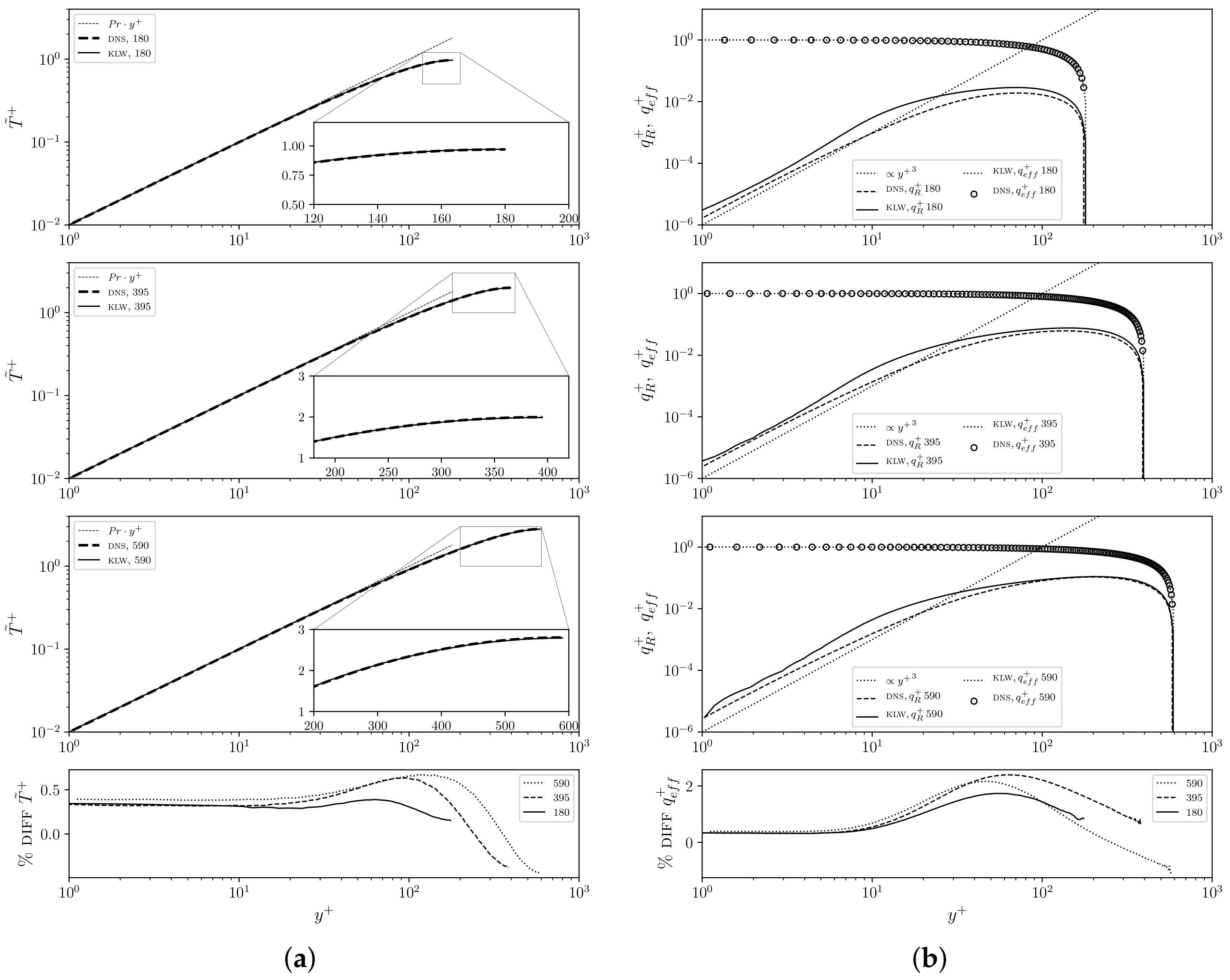
The non-dimensional mean temperature profiles ${\tilde{T}}^{+}$ are shown in Figure 2a for all the simulated cases. We see that the numerical results match the linear behavior ${\tilde{T}}^{+}=Pr{y}^{+}$ and the relative DNS data.

In Figure 2b we report the profiles of the non-dimensional turbulent heat flux ${\mathbf{q}}_R^{+}·\widehat{n}=\langle u^{\prime +}{T}^{\prime +}\rangle$, where $\widehat{n}$ is the unit vector normal to the wall surface, and of the total non-dimensional heat flux $q_{eff}^{+}$ = $({\mathbf{q}}_R^{+}+{\mathbf{q}}^{+})·\widehat{n}$. In the viscous region the non-dimensional heat flux profiles agree with the reference behavior, i.e.,

$$\langle u^{\prime +}{T}^{\prime +}\rangle \propto {\left(y^{+}\right)}^3,$$

which is obtained in the case of zero temperature fluctuations on the heated wall. In fact, from the near wall behaviors described in Table 2, it follows

$$\langle u^{\prime +}{T}^{\prime +}\rangle =(b_2{y}^2+\dots )·(d_0+d_{1}y+\dots ).$$

Having imposed null temperature fluctuations on the heated wall, the value of $d_0$ is equal to zero, so $\langle u^{\prime +}{T}^{\prime +}\rangle =b_2{d}_1{y}^3+\dots$, with $b_2$ and $d_1$ being unknown coefficients. As for the case of non-dimensional velocity and Reynolds stress component, a quantitative analysis is reported with the percentage difference plots shown on the bottom of Figure 2. For the non-dimensional temperature, the agreement is very satisfactory, with a diff value in the range $[-0.25\%;0.5\%]$, while for the total non-dimensional heat flux the difference with DNS is in the range [−0.5%, 2.5%]. In particular, in the viscous and buffer regions the computed turbulent heat flux overestimates the reference values. Since the turbulent heat flux is computed as $\langle u^{\prime }{T}^{\prime }\rangle ={\alpha }_t{T}_{,x}$ and the temperature profile perfectly matches the reference one, the overestimation of the heat flux is due to the modeled value of the eddy thermal diffusivity. At low Reynolds, in order to capture these components, an appropriate non-isotropic model may be needed. However this difference in the turbulent heat flux does not influence the temperature profile because the molecular heat flux has a great importance for these very low Prandtl and Reynolds numbers, and for very high $y^{+}$ (see [5]), as can be seen from the comparison of $q_R^{+}$ and $q_{eff}^{+}$.

3.2. Cylindrical Pipe Tests

With the reference to a duct geometry that consists of a cylinder with a diameter $D=0.0605$ m, we simulate several cases of fully developed turbulent flows with both $Pr=0.01$ and $Pr=0.025$. A summary of these cases is reported in

Table 6. Cylindrical pipe tests. Summary table and labels for different simulated cases.

Case	A	B	C	D	E	F	G
$R{e}_{\tau }$	180	360	550	1000	3580	5840	6860
$Re$	5760	12,770	20,700	41,000	165,000	286,000	341,000

together with the relative value of the turbulent Reynolds number $R{e}_{\tau }$ and of the Reynolds number $Re$.

On the wall surface, a uniform heat flux q per unit area is applied with value of $3.6\times {10}^5$ W/m${}^2$. As for the case of plane channel, we denote with ${\mathsf{\Gamma }}_w$ the wall surface; with ${\mathsf{\Gamma }}_{in}$ and ${\mathsf{\Gamma }}_{out}$ the inlet and outlet sections; and with ${\mathsf{\Gamma }}_{sym}$ the cylinder axis which is the axial symmetry axis of the problem. The boundary conditions are reported in

Table 7. Cylindrical pipe tests. Boundary conditions.

Var.	${\mathsf{\Gamma }}_{\mathit{sym}}$	${\mathsf{\Gamma }}_{\mathit{in}}\cup {\mathsf{\Gamma }}_{\mathit{out}}$	${\mathsf{\Gamma }}_{\mathit{w}}$
u	$u=0$	$\frac{\partial u}{\partial y}=0$	$u=0$
v	$\frac{\partial v}{\partial r}=0$	$\frac{\partial v}{\partial y}=0$	$\frac{\partial v}{\partial r}=\frac{\mu }{\delta }$
k	$\frac{\partial k}{\partial r}=0$	$\frac{\partial k}{\partial y}=0$	$\frac{\partial k}{\partial r}=\frac{2k}{\delta }$
$\mathsf{\Omega }$	$\frac{\partial \mathsf{\Omega }}{\partial r}=0$	$\frac{\partial \mathsf{\Omega }}{\partial y}=0$	$\mathsf{\Omega }=ln\left(\frac{2\nu }{C_{\mu }{\delta }^2}\right)$
$\tilde{T}$	$\frac{\partial \tilde{T}}{\partial r}=0$	$\frac{\partial \tilde{T}}{\partial y}=0$	$\tilde{T}=0$
$k_{\theta }$	$\frac{\partial k_{\theta }}{\partial r}=0$	$\frac{\partial k_{\theta }}{\partial y}=0$	$\frac{\partial k_{\theta }}{\partial r}=\frac{2k_{\theta }}{\delta }$
${\mathsf{\Omega }}_{\theta }$	$\frac{\partial {\mathsf{\Omega }}_{\theta }}{\partial r}=0$	$\frac{\partial {\mathsf{\Omega }}_{\theta }}{\partial y}=0$	${\mathsf{\Omega }}_{\theta }=ln\left(\frac{2\alpha }{C_{\mu }{\delta }^2}\right)$

, where r is the radial coordinate, u its component of the mean velocity field and v the axial one.

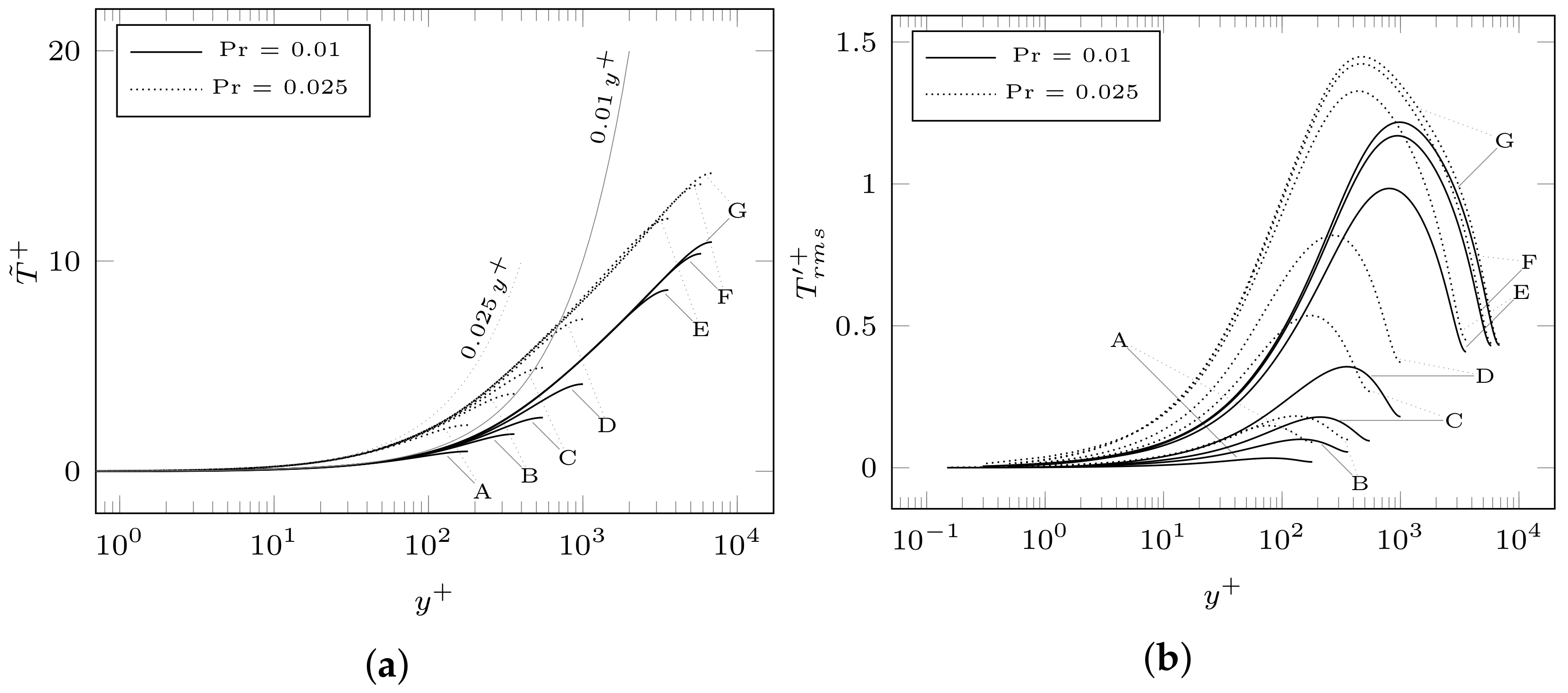
The physical properties are shown in Table 4 where we consider two fluids with different Prandtl numbers. We implement the modified KLW model and also the Kays correlation in the same numerical code. The same test cases are carried out for this model and the same comparison with the experimental correlations is given. In this way we intend to compare two different thermal turbulence models using the same numerical code and the same model for the dynamical turbulence, thereby allowing us to highlight the differences obtained in the simulated heat transfer performances, which are then due only to the different thermal turbulence models. In Figure 3a the non-dimensional temperature ${\tilde{T}}^{+}$ profiles are reported for the simulated cases. We see that the simulations match the linear behavior ${\tilde{T}}^{+}=Pr{y}^{+}$, in accordance with the near wall behavior described in Table 2. In Figure 3b the non-dimensional root-mean-squared temperature fluctuation $k_{\theta }$ is shown as a function of non-dimensional wall distance $y^{+}$ for all the simulated cases and for both $Pr=0.01$ and $0.025$. We can see how the different molecular Prandtl numbers affect the temperature fluctuations. In fact, for any given Reynolds number, the simulations with $Pr=0.01$ are characterized by a maximum value of $T_{rms}^{\prime +}$ which is smaller than the one obtained with $Pr=0.025$ and the peak position is shifted nearer the pipe’s middle axis. In

Table 8. Cylindrical pipe tests. Mean values across the transverse section of the pipe: RMS temperature fluctuations $T_{rms,m}^{\prime +}$, mean temperature ${\tilde{T}}_m^{+}$ and the ratio $T_{rms,m}^{\prime +}/{\tilde{T}}_m^{+}$.

Case	${\mathit{Re}}_{\mathit{\tau }}$	$\mathit{Pr}=0.01$			$\mathit{Pr}=0.025$
		${\tilde{\mathit{T}}}_{\mathit{m}}^{+}$	${\mathit{T}}_{\mathit{rms},\mathit{m}}^{\prime +}$	${\mathit{T}}_{\mathit{rms},\mathit{m}}^{\prime +}$/${\tilde{\mathit{T}}}_{\mathit{m}}^{+}$	${\tilde{\mathit{T}}}_{\mathit{m}}^{+}$	${\mathit{T}}_{\mathit{rms},\mathit{m}}^{\prime +}$	${\mathit{T}}_{\mathit{rms},\mathit{m}}^{\prime +}$/${\tilde{\mathit{T}}}_{\mathit{m}}^{+}$
A	180	0.62	0.025	0.041	1.46	0.112	0.076
B	360	1.17	0.075	0.064	2.53	0.275	0.108
C	550	1.71	0.134	0.078	3.44	0.402	0.117
D	1000	2.82	0.268	0.095	5.16	0.609	0.117
E	3578	6.35	0.711	0.111	9.30	0.895	0.096
F	5843	7.85	0.814	0.103	10.82	0.896	0.082
G	6852	8.34	0.836	0.100	11.32	0.918	0.081

we report the mean values across the pipe transverse section of non-dimensional mean temperature and non-dimensional RMS temperature fluctuations

$${\tilde{T}}_m^{+}=\frac{2}{D}\underset{0}{\overset{D/2}{\int }}{\tilde{T}}^{+}dr{T}_{rms,m}^{\prime +}=\frac{2}{D}\underset{0}{\overset{D/2}{\int }}{T}_{rms}^{\prime +}dr,$$

(35)

together with their ratio $T_{rms,m}^{\prime +}/{\tilde{T}}_m^{+}$. These parameters allow us to compare the mean temperature fluctuations modulus with the average difference between the fluid and the solid temperatures. For low velocities, i.e., with $R{e}_{\tau }\le 1000$, we see that the temperature fluctuations increase for increasing mean velocities and are higher for $Pr=0.025$ than for $Pr=0.01$. For the cases $R{e}_{\tau }>1000$ we observe that the importance of the temperature fluctuations, relative to the mean temperature, decreases for increasing velocities and that it is higher for $Pr=0.01$ than for $Pr=0.025$.

For forced convection flows and high Reynolds numbers DNS simulations are not available and only experimental data can be compared with the results obtained with the KLW model. As a consequence, temperature profiles actually cannot be captured from liquid-metal experiments, and only integral measurements, i.e., Nusselt number values and heat transfer coefficients, are available. Nusselt numbers usually define the heat transfer coefficients between a wall surface and a fluid flow as

$$Nu=\frac{h{D}_h}{\lambda },$$

(36)

where $\lambda$ is the thermal conductivity, $D_h$ the hydraulic diameter and h the convective heat transfer coefficient. If a constant heat flux q is applied on wall surfaces, the convective heat transfer coefficient h can be written as

$$h=\frac{q}{T_w-T_b},$$

(37)

where $T_w$ is the wall surface temperature and $T_b$ is the bulk temperature of the fluid defined as

$$T_b=\frac{{\int }_{A}T\mathbf{u}·\widehat{n}dA}{{\int }_A\mathbf{u}·\widehat{n}dA},$$

(38)

where the unit vector normal is denoted by $\widehat{n}$ and A is the channel cross section.

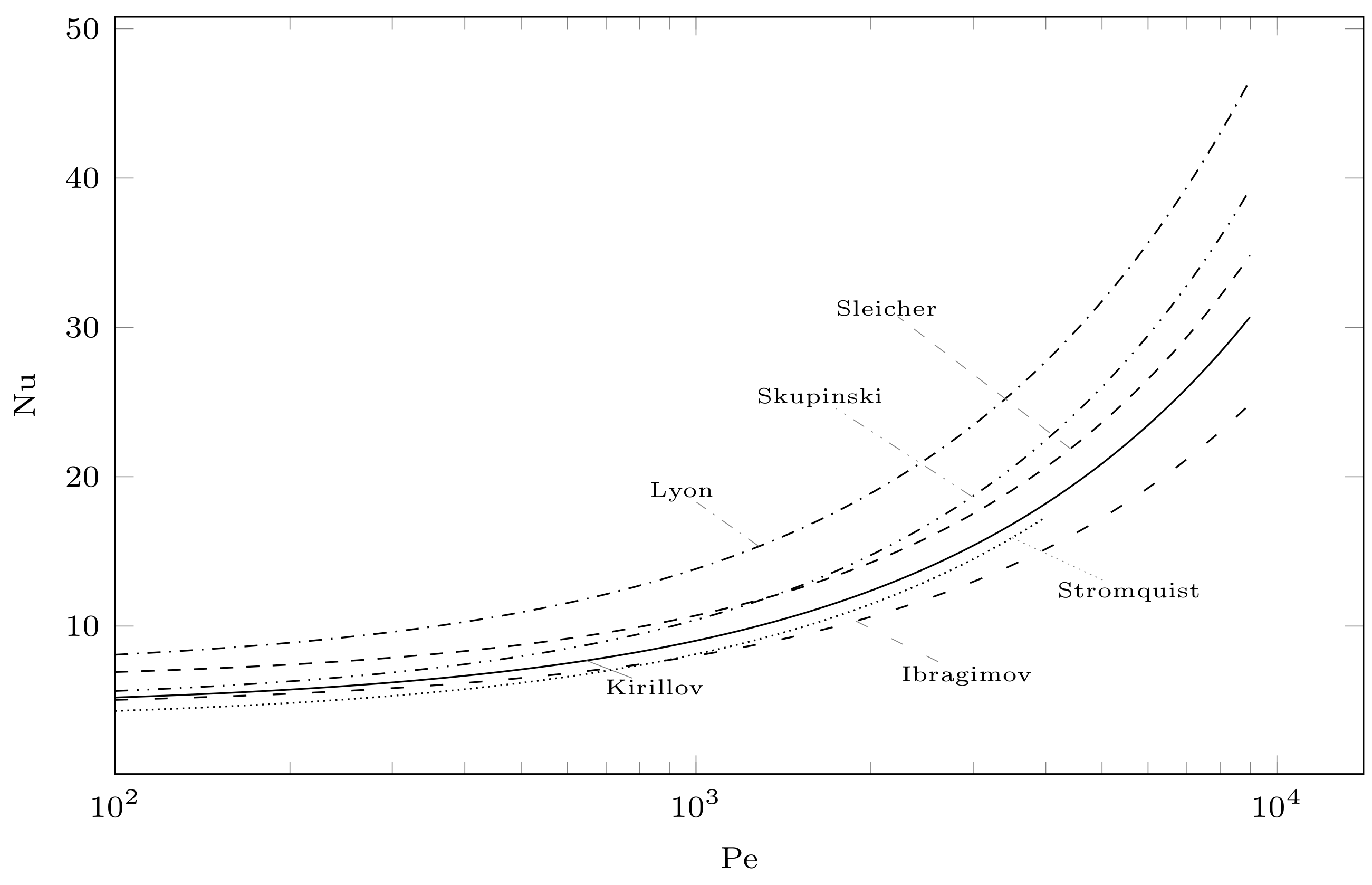
Experimental data summarize their results in the form of correlations for each type of geometry as a function of the Peclet number $\mathit{Pe}=\mathit{Pr}·\mathit{Re}$. Many experimental correlations are known for liquid metals, but unfortunately many of them do not agree. One can easily see that there is a disagreement between the different experiments and authors have attempted many explanations for this discrepancy; see for example, [4]. The general expressions of these correlations for the cylindrical pipe geometry take the following form:

$$Nu=A+aP{e}^n,$$

(39)

where a and n are constant assumed to be positive numbers. As said before, there are many different experimental correlations and each correlation comes from a different experiment that brings its own range of validity expressed in terms of Reynolds numbers. Some of these well known correlations are reported as

$$\begin{array}{ccccc}\hfill & \mathit{Lyon}\hfill & \hfill & Nu=7.0+0.025{\left(\frac{Pe}{P{r}_t}\right)}^{0.8}\hfill & \hfill {10}^4\le Re\le 5·{10}^6,\end{array}$$

(40)

$$\begin{array}{ccccc}\hfill & \mathit{Skupinski}\hfill & \hfill & Nu=4.82+0.0185P{e}^{0.827}\hfill & \hfill {10}^4\le Re\le 5·{10}^6,\end{array}$$

(41)

$$\begin{array}{ccccc}\hfill & \mathit{Sleicher}\hfill & \hfill & Nu=6.3+0.0167P{e}^{0.85}P{r}^{0.08}\hfill & \hfill {10}^4\le Re\le 5·{10}^6,\end{array}$$

(42)

$$\begin{array}{ccccc}\hfill & \mathit{Ibragimov}\hfill & \hfill & Nu=4.5+0.014P{e}^{0.8}\hfill & \hfill {10}^4\le Re\le 5·{10}^6,\end{array}$$

(43)

$$\begin{array}{ccccc}\hfill & \mathit{Stromquist}\hfill & \hfill & Nu=3.6+0.018P{e}^{0.8}\hfill & \hfill 88\le Pe\le 4000.\end{array}$$

(44)

$$\begin{array}{ccccc}\hfill & \mathit{Kirillov}\hfill & \hfill & Nu=4.5+0.018P{e}^{0.8}\hfill & \hfill {10}^4<Re<5·{10}^6.\end{array}$$

(45)

The correlations in Equations (40)–(45) can be seen in Figure 4. Each correlation has a name related to its investigator, as labeled in Figure 4. In this Figure, correlation data from different experiments, such as lead, lead-bismuth, bismuth and sodium, are mixed with the aim to obtain a law valid for all liquid metals. The interested reader can see details for each experiment in [29,30,31,32,33,34,35,36]. For low values of Peclet numbers ($Pe<1000$) the Kirillov curve is the correlation that fits better all the experimental points [4,34]. In [4] the authors proposed the following new correlation

$$\begin{array}{cc}\hfill & Nu=A+0.018P{e}^{0.8},\hfill \\ \hfill & A=\left\{\begin{array}{cc}\hfill & 4.5Pe<1000,\hfill \\ \hfill & 5.4-9\times {10}^{-4}Pe1000\le Pe\le 2000,\hfill \\ \hfill & 3.6Pe>2000.\hfill \end{array}\right.\hfill \end{array}$$

(46)

It is easy to see that this correlation matches the Kirillov correlation in the low Peclet region while it tends to the Stromquist one in the range of high Peclet numbers. In Figure 5 we compare the values of $Nu$ obtained with the KLW and with Kays models for simulations in the range $80<Pe<10000$ with $Pr=0.025$ and $0.01$ with Kirillov and Cheng correlations. The same data are shown in

Table 9. Cylindrical pipe tests. Numerical comparison of the KLW and Kays [13] models with Kirillov [33] and  Cheng [4] correlations for $Pr=0.025$ and $0.01$.

Pr	Source	Reynolds Number
		341,360	285,800	165,400	41,000	20,680	12,760	5760
0.025	KLW	29.4092	26.1685	18.5608	9.2123	7.5382	6.6523	5.6329
	Kays	42.9137	38.1888	27.0105	12.4689	9.3894	7.9416	6.3323
	Kirillov	29.6295	26.3008	18.5779	9.1108	7.1690	6.3135	5.4593
	Cheng	28.7295	25.4008	17.6779	9.0885	7.1690	6.3135	5.4593
0.01	KLW	15.9311	14.4070	10.8496	6.7213	6.0596	5.7411	5.3430
	Kays	22.9363	20.7126	15.4458	8.6137	7.1788	6.5008	5.7193
	Kirillov	16.6110	15.0068	11.2848	6.7221	5.7863	5.3740	4.9623
	Cheng	15.7110	14.1068	10.6900	6.7221	5.7863	5.3740	4.9623

as functions of different $Pr$ and $Re$ numbers.

The KLW model, for $Pr=0.025$, matches close to the Kirillov correlation when $Pe>1000$, while some difference can be seen for $Pr=0.01$. The KLW model lays between Kirillov and the Cheng correlations, in the high Peclet region, while in the low Peclet region the model overestimates the values. From Figure 5 it can be seen that the Nusselt number values obtained from the KLW model, in both $Pr=0.01$ and $Pr=0.025$ cases, lay in the range $[0,+5\%]$ with respect to the Cheng correlation. As it regards the Kays model, we can see that for low Peclet and Prandtl numbers the results are greater than those obtained with KLW model and predicted by both correlations, while with increasing Peclet the mismatch becomes very large, with Nusselt number values lying in the range $[+30\%;+50\%]$ with respect to Cheng correlation. When eddy viscosity ratio increases, namely, for high Peclet numbers, the average turbulent Prandtl, given by Equation (23), tends to $0.85$, which is known to be inaccurate for predicting this type of flow.

4. Conclusions

In this work we have extended the investigation of heat turbulence modeling to a wider range of low-Prandtl numbers characteristic of liquid-metal flows. The investigation, which presents a two-equation logarithmic k-$\mathsf{\Omega }$-$k_{\theta }$-${\mathsf{\Omega }}_{\theta }$ model, includes forced flow studies with both low Peclet numbers, where only DNS simulations are available, and high Peclet numbers where only experimental results are available. Two approaches have been compared, a Kays model and a logarithmic k-$\mathsf{\Omega }$-$k_{\theta }$-${\mathsf{\Omega }}_{\theta }$ turbulence model, to be used in engineering applications with low-high Peclet numbers. Since only DNS results are available, for low-Peclet-number, in plane and channel geometries, we have compared them for sodium and lead’s characteristic Prandtl numbers. The comparison between the numerical results obtained with the four-parameter turbulence model with DNS data and experimental correlations can be considered satisfactory for a wide range of Peclet numbers and for both the Prandtl numbers studied. On the other hand, the Kays model does not seem to be able to adapt to the study of all these different cases, especially for high Peclet numbers, and a two-equation model for the heat turbulent diffusivity seems necessary.

References

- Grötzbach, G. Challenges in low-Prandtl number heat transfer simulation and modeling. Nucl. Eng. Des. 2013, 264, 41–55. [Google Scholar] [CrossRef]
- Marocco, L.; Cammi, G.; Flesch, J.; Wetzel, T. Numerical analysis of a solar tower receiver tube operated with liquid metals. Int. J. Therm. Sci. 2016, 105, 22–35. [Google Scholar] [CrossRef]
- Fazio, C. (Ed.) Handbook on Lead-Bismuth Eutectic Alloy and Lead Properties, Materials Compatibility, Thermal-hydraulics and Technologies; OECD: Paris, France, 2015. [Google Scholar]
- Cheng, X.; Tak, N.i. Investigation on turbulent heat transfer to lead–bismuth eutectic flows in circular tubes for nuclear applications. Nucl. Eng. Des. 2006, 236, 385–393. [Google Scholar] [CrossRef]
- Duponcheel, M.; Bricteux, L.; Manconi, M.; Winckelmans, G.; Bartosiewicz, Y. Assessment of RANS and improved near-wall modeling for forced convection at low Prandtl numbers based on LES up to Reτ = 2000. Int. J. Heat Mass Transf. 2014, 75, 470–482. [Google Scholar] [CrossRef]
- Bricteux, L.; Duponcheel, M.; Winckelmans, G.; Tiselj, I.; Bartosiewicz, Y. Direct and large eddy simulation of turbulent heat transfer at very low Prandtl number: Application to lead-bismuth flows. Nucl. Eng. Des. 2012, 246, 91–97. [Google Scholar] [CrossRef]
- Shams, A.; Roelofs, F.; Baglietto, E.; Lardeau, S.; Kenjeres, S. Assessment and calibration of an algebraic turbulent heat flux model for low-Prandtl fluids. Int. J. Heat Mass Transf. 2014, 79, 589–601. [Google Scholar] [CrossRef]
- Manservisi, S.; Menghini, F. A CFD four parameter heat transfer turbulence model for engineering applications in heavy liquid metals. Int. J. Heat Mass Transf. 2014, 69, 312–326. [Google Scholar] [CrossRef]
- Kawamura, H.; Abe, H.; Matsuo, Y. DNS of turbulent heat transfer in channel flow with respect to Reynolds and Prandtl number effects. Int. J. Heat Fluid Flow 1999, 20, 196–207. [Google Scholar] [CrossRef]
- Tiselj, I.; Cizelj, L. DNS of turbulent channel flow with conjugate heat transfer at Prandtl number 0.01. Nucl. Eng. Des. 2012, 253, 153–160. [Google Scholar] [CrossRef]
- Hoyas, S.; Jiménez, J. Reynolds number effects on the Reynolds-stress budgets in turbulent channels. Phys. Fluids 2008, 20, 101511. [Google Scholar] [CrossRef] [Green Version]
- Lozano-Durán, A.; Jiménez, J. Effect of the computational domain on direct simulations of turbulent channels up to Reτ = 4200. Phys. Fluids 2014, 26, 011702. [Google Scholar] [CrossRef]
- Kays, W. Turbulent Prandtl number. Where are we? J. Heat Transf. 1994, 116, 284–295. [Google Scholar] [CrossRef]
- Hwang, C.; Lin, C. A low Reynolds number two-equation kt-et model to predict thermal field. Int. J. Heat Mass Transf. 1999, 42, 3217–3230. [Google Scholar] [CrossRef]
- Abe, K.; Suga, K. Towards the development of a Reynolds-averaged algebraic turbulent scalar-flux model. Int. J. Heat Fluid Flow 2001, 22, 19–29. [Google Scholar] [CrossRef]
- Abe, K.; Kondoh, T.; Nagano, Y. A new turbulence model for predicting fluid flow and heat transfer in separating and reattaching flows I. Flow field calculations. Int. J. Heat Mass Transf. 1994, 37, 139–151. [Google Scholar] [CrossRef]
- Nagano, Y.; Shimada, M. Development of a two equation heat transfer model based on direct simulations of turbulent flows with different Prandtl numbers. Phys. Fluids 1996, 8, 3379–3402. [Google Scholar] [CrossRef]
- Abe, K.; Kondoh, T.; Nagano, Y. A new turbulence model for predicting fluid flow and heat transfer in separating and reattaching flows II. Thermal field calculations. Int. J. Heat Mass Transf. 1995, 38, 1467–1481. [Google Scholar] [CrossRef]
- Manservisi, S.; Menghini, F. Triangular rod bundle simulations of a CFD k-ε-kθ-εθ heat transfer turbulence model for heavy liquid metals. Nucl. Eng. Des. 2014, 273, 251–270. [Google Scholar] [CrossRef]
- Manservisi, S.; Menghini, F. CFD simulations in heavy liquid metal flows for square lattice bare rod bundle geometries with a four parameter heat transfer turbulence model. Nucl. Eng. Des. 2015, 295, 251–260. [Google Scholar] [CrossRef]
- Cerroni, D.; Vià, R.D.; Manservisi, S.; Menghini, F.; Pozzetti, G.; Scardovelli, R. Numerical validation of a k-ω-kθ-ωθ heat transfer turbulence model for heavy liquid metals. J. Phys. Conf. Ser. 2015, 655, 012046. [Google Scholar] [CrossRef]
- Da Vià, R.; Manservisi, S.; Menghini, F. A k-Ω-kθ-Ωθ four parameter logarithmic turbulence model for liquid metals. Int. J. Heat Mass Transf. 2016, 101, 1030–1041. [Google Scholar] [CrossRef]
- Ilinca, F.; Hetu, J.; Pelletier, D. A unified finite element algorithm for two-equation models of turbulence. Comput. Fluids 1998, 27, 291–310. [Google Scholar] [CrossRef]
- Da Vià, R.; Manservisi, S. Numerical simulation of forced and mixed convection turbulent liquid sodium flow over a vertical backward facing step with a four parameter turbulence model. Int. J. Heat Mass Transf. 2019, 135, 591–603. [Google Scholar] [CrossRef]
- Wilcox, D.C. Turbulence Modeling for CFD, 3rd ed.; DCW Industries, Inc.: La Cañada, CA, USA, 2006. [Google Scholar]
- Hanjalić, K.; Launder, B. Modelling Turbulence in Engineering and the Environment; Cambridge University Press: New York, NY, USA, 2011. [Google Scholar]
- Hattori, H.; Nagano, Y.; Tagawa, M. Analysis of turbulent heat transfer under various thermal conditions with two-equation models. Eng. Turbul. Model. Exp. 2014, 2, 43–52. [Google Scholar]
- Official Repository for Multigrid Finite Element Code FEMuS, Github Link. Available online: https://github.com/FemusPlatform/femus (accessed on 23 June 2020).
- Lyon, R. Liquid metal heat transfer coefficients. Chem. Eng. Prog. 1951, 47, 75–79. [Google Scholar]
- Lyon, R. Liquid-Metals Handbook; Atomic Energy Comm.: Oak Ridge, TN, USA, 1952. [Google Scholar]
- Ibragimov, M.; Subbotin, V.; Ushakov, P. Investigation of heat transfer in the turbulent flow of liquid metals in tubes. At. Energiya 1960, 8, 54–56. [Google Scholar]
- Stromquist, W.K. Effect of Wetting on Heat Transfer Characteristics of Liquid Metals; University of Tennessee: Knoxville, TN, USA, 1953. [Google Scholar]
- Kirillov, P.; Ushakov, P. Heat transfer to liquid metals: Specific features, methods of investigation, and main relationships. Therm. Eng. 2001, 48, 50–59. [Google Scholar]
- Johnson, H.; Hartnett, J.; Clabaugh, W. Heat transfer to molten lead–bismuth eutectic in turbulent pipe flow. Trans. Am. Soc. Mech. Eng. 1953, 75, 1191–1198. [Google Scholar]
- Skupinski, E.; Tortel, J.; Vautrey, L. Determination des coefficients de convection d’un alliage sodium-potassium dans un tube circulaire. Int. J. Heat Mass Transf. 1965, 8, 937–951. [Google Scholar] [CrossRef]
- Sleicher, C.A.; Awad, A.S.; Notter, R.H. Temperature and eddy diffusivity profiles in NaK. Int. J. Heat Mass Transf. 1973, 16, 1565–1575. [Google Scholar] [CrossRef]
Figure 1.
Two-dimensional channel tests (). Non-dimensional mean axial velocity profiles (a) and non-dimensional Reynolds stresses (b) as a function of the non-dimensional wall distance . Results obtained with KLW model are compared with DNS data [10]. The quantitative analysis (plots on bottom) show the percentage difference computed between the KLW and DNS results for and .
Figure 2.
Two-dimensional channel tests (). Non-dimensional mean temperature profiles (a) and non-dimensional turbulent heat flux and total heat flux (b) as a function of the non-dimensional distance from the wall . The results obtained with KLW model are compared with DNS data [10]. On the bottom, quantitative comparisons with DNS data for and .
Figure 3.
Cylindrical pipe tests (KLW model). Non-dimensional profiles of the mean temperature (a) and the root-mean-squared temperature fluctuations (b) as a function of the non-dimensional distance from the wall with and . The cases A, B, C, D, E, F and G are defined in Table 6.
Figure 4.
Cylindrical pipe tests (constant heat flux). Nusselt numbers from different experimental data in Equations (40)–(45) as a function of the Peclet number.
Figure 5.
Cylindrical pipe tests. Nusselt number values for the simulations performed for fluids with and with the KLW and Kays [13] models. The values are compared with the Kirillov [33] and Cheng [4] correlations.