Article

Delineation of Management Zones for Site-Specific Information about Soil Fertility Characteristics through Proximal Sensing of Potato Fields

1
Faculty of Sustainable Design Engineering, University of Prince Edward Island, Charlottetown, PE C1A 4P3, Canada
2
School of Climate Change and Adaptation, University of Prince Edward Island, Charlottetown, PE C1A 4P3, Canada
3
Engineering Department, Dalhousie University Agriculture Campus, Truro, NS B2N 5E3, Canada
*
Authors to whom correspondence should be addressed.
Agronomy 2020, 10(12), 1854; https://doi.org/10.3390/agronomy10121854
Submission received: 19 October 2020 / Revised: 18 November 2020 / Accepted: 21 November 2020 / Published: 25 November 2020
(This article belongs to the Section Agricultural Biosystem and Biological Engineering)

Abstract

:
The delineation of management zones (MZs) has been suggested as a solution to mitigate adverse impacts of soil variability on potato tuber yield. This study quantified the spatial patterns of variability in soil and crop properties to delineate MZs for site-specific soil fertility characterization of potato fields through proximal sensing of fields. Grid sampling strategy was adopted to collect soil and crop data from two potato fields in Prince Edward Island (PEI). DUALEM-2 sensor, Time Domain Reflectometry (TDR-300), GreenSeeker were used to collect soil ground conductivity parameter horizontal coplanar geometry (HCP), soil moisture content (θ), and normalized difference vegetative index (NDVI), respectively. Soil organic matter (SOM), soil pH, phosphorous (P), potash (K), iron (Fe), lime index (LI), and cation exchange capacity (CEC) were determined from soil samples collected from each grid. Stepwise regression shortlisted the major properties of soil and crop that explained 71 to 86% of within-field variability. The cluster analysis grouped the soil and crop data into three zones, termed as excellent, medium, and poor at a 40% similarity level. The coefficient of variation and the interpolated maps characterized least to moderate variability of soil fertility parameters, except for HCP and K that were highly variable. The results of multiple means comparison indicated that the tuber yield and HCP were significantly different in all MZs. The significant relationship between HCP and yield suggested that the ground conductivity data could be used to develop MZs for site-specific fertilization in potato fields similar to those used in this study.

1. Introduction

The potato (Solanum tuberosum L.) is the world’s third most consumed food, which is produced in all continents except Antarctica [1]. Potatoes are produced above 19 million hectares worldwide, Canada being ahead of many countries in its potato production. Two Atlantic Canadian provinces, including Prince Edward Island and New Brunswick, contribute 24.5% and 13.6%, respectively, in the total potato production of Canada [2]. However, the yield per unit area of potatoes in these provinces is less than that of most American States, emphasizing the need for better management of potato cultivation in Canada.
For precise management of crop production within-field, it is very important to know about the spatial variability of crop and soil properties [3]. Several soil properties have been identified as influencing potato yield, including soil texture [4], soil water content [5], and organic matter content [6]. The within-field variability of soil and crop properties is important to optimize productivity and reduce environmental risks. As there exists spatial variability within the fields, precision agriculture (PA) uses information technology to manage crop production by considering the variations within-field, and increase crop productivity and sustainability [7]. Data acquisition, management, analysis, and processing/modeling is vital for sustainable agriculture in order to ensure meeting future food safety challenges [8]. Reductions in crop productivity can—directly or indirectly—be accredited to several factors, such as inadequate nutrient availability, insufficient crop and soil management practices, unpleasant weather conditions, the occurrence of pests and diseases, and water deficiency [9,10,11,12]. Spatially variable fertilizer application can manage these problems, while being economically viable and environment friendly [13]. Despite the choice of cultivar, plant protection, and constant water supply, a further, important agronomic measure for potato production is adequate, and site-specific nutrient supply [14].
Efficient nutrient management for better soil health requires understanding of available technologies; for example, for site-specific nutrient management [15]. Developing variable rate fertilizer application maps is significant in applying PA techniques. One effective PA technique is delineation of management zones (MZs) [16]. The cost of inputs and their impact on surrounding environment can be minimized by the customized application of these inputs in different parts of the field through MZs [17]. Yield, fertility, and geographical maps can be used to form MZs for site-specific fertigation. This application can enhance the crop yield and farmer profit. Development of these maps for soil properties, plant characteristics, and yield by using grid sampling is a significant feature of PA [18]. Precision agriculture plays an important role in achieving sustainable agriculture [19] and the use of MZs is an important aspect of PA [20]. The most popular approach to manage spatial variability within fields is the use of MZs, which are field subdivisions, and can be used to direct variable rate fertilizer application [16].
There are different methods for delineating MZs; e.g., soil mapping [21] from the data collected through proximal sensing of fields [22]. Variables, including soil electrical conductivity, yield statistics, soil texture, topography, soil organic matter (SOM), and different soil nutrients, have all been used to delineate MZs. The MZs are delineated by dividing the field into different areas. Some of the areas have different responses, whereas others may show the same behaviors [23]. The delineation of MZs for PA based on cluster analysis has been verified to be effective to combine the impacts of different variables on the outcome [24].The analysis is based on finding dissimilarities among observations by using a clustering algorithm through partitioning or hierarchical methods [25]. In addition to this, the use of MZs is a promising approach to fertilizer management in intensive potato production in Canadian provinces including Quebec [26,27], New Brunswick, and Prince Edward Island [28]. However, the soils of Prince Edward Island have special characteristics of presence of gravels [29], slope leading to variations in soil moisture content (θ) [30], and varying SOM [31]. The purpose of this study was to quantify the spatial patterns of variability in soil and crop properties in Prince Edward Island (PEI). To achieve this purpose, it was hypothesized that delineation of MZs would help in quantifying spatial patterns of variability in soil and crop properties.

2. Material and Methods

Two potato fields were selected in Souris, PEI, Canada, during the growing seasons of 2017 and 2018. The experimental field of the 2017 growing season is referred to as Field 1 (46.3550° N, 62.2518° W) and the field used during the 2018 growing season is referred to as Field 2 (46.7071° N, 64.2269° W) from here onwards (Figure 1). The two fields are approximately 5 km apart from one another. The same fields could not be selected during the second year of study due to the crop rotation strategy in Prince Edward Island. Both fields were managed according to conventional practices in the region. Fertility and pest management was applied according to provincial recommendations. A common potato variety Russet Burbank was cultivated. The potato seeds were sown on 18 May 2017 in Field 1 and 19 May 2018 in Field 2.
A grid sampling approach was established by determining the coordinates of grids with Real-Time Kinematic Global Position System (RTK-GPS) (Benchmark, Calgary, AB, Canada). The horizontal coplanar geometry (HCP) of the field was measured using ground conductivity surveys with DUALEM-2 sensor (DUALEM Inc., Milton, ON, Canada) in both fields. The grid pattern for sampling was one-third, or half of the range of variability [32], based on which a grid size of 25 m × 25 m was fixed for Field 1 (n = 40) and Field 2 (n = 39); where n is the number of grids nodes).
Soil samples (about 500 g each) were collected from each grid from a 15 cm depth with a soil auger prior to sowing. The soils of PEI potato fields are sandy loams (Orthic Humo-Ferric Podzol) with large gravels and stones contents, and with more than 2% of SOM. The sandy soils have good drainage, aeration, and thus can result in drought stress in absence of supplemental irrigation. However, sandy loam soils with adequate presence of SOM can retain θ and do not drain as rapidly. Potatoes prefer a well-drained, medium textured and loose loam, fertile soil that is high in organic matter [33].
Post-sowing data collection was done twice during the growing season. For Field 1, the first and second samplings were on 8 June 2017 and 13 July 2017, respectively. For Field 2, the first and second samplings were on 11 June 2018 and 10 July 2018, respectively. At each sampling time, HCP was measured using DUALEM-2 sensor. A FieldScout TDR-300 probe (Spectrum Technologies, Inc., Aurora, CO, USA) was used to measure θ at each soil sampling point by inserting TDR rods to 15 cm depths. The data for normalized difference vegetative index (NDVI) and yield were collected at the end of growing seasons. GreenSeeker™ handheld sensor was used to measure NDVI. To collect the tuber yield samples a 1 m × 1 m plot was dug manually in each grid. A digital weighing balance was used to weigh those samples. After yield measurements, tubers were buried back in soil for farmers to collect their farm yield. Harvesting was performed on 2 October 2017 and 4 October 2018 in Fields 1 and 2, respectively.
The soil samples were analyzed for SOM, soil pH, θ, P, K, Fe, CEC, and LI. Phosphorus was measured using Olsen method [34], K using Flame photometric method [35], Fe with colorimetric method [36], CEC with BaCl2- compulsive exchange procedure [37], and pH was determined using a pH multimeter. The LI was determined by mixing the SMP buffer solution with soil and followed by measuring its pH [38]. Soil organic matter was determined using standard methods [39,40]. Five grams of ground air-dried soil <2 mm diameter were placed in 15 mL ceramic cups and oven-dried at 105 °C for 24 h and cooled in a desiccator before weighing for its mass (M105) prior to combusting it for 5 h at 550 °C in a muffle furnace. The soil was then cooled down to 105 °C before putting it in a desiccator for further cooling down. The cooled samples were weighed again for their mass (M550) to determine SOM, using a formula introduced by [41].
S O M ( % ) = ( M 105 M 550 M 105 ) × 100

Statistical Analysis

Values of the mean, maximum, minimum, coefficient of variance (CV), and variance were calculated for all the crop and soil properties using Minitab 18 (Minitab, INC., State College, PA, USA). Minitab provides numerous statistical analysis tools helpful for conducting regression, analysis of variance (ANOVA), and other statistical measures [42]. Stepwise regression, which is a method of fitting regression models while making choice of predictive variables, was conducted in Minitab. In each step, a variable (from the list of variables given in Table 1 and Table 2) were considered for addition to or subtraction from the set of explanatory variables mentioned in Equations (1)–(4), based on values of coefficient of determination (R2) of the regression models. Stepwise regression helped in assessing the overall contribution of all soil properties toward soil variability in a Fields 1 and 2. Stepwise regression was performed, which reduced the number of parameters to have ones with more effect on the variability. Coefficient of variation (CV) is the first indicator of variability. If the CV < 15%, it means the parameter is the least variable; if CV = 15–35%, it means the parameter is moderately variable. If the CV > 35%, it means the parameter is highly variable [43]. Geostatistical analysis was performed using GeoStatistics Software (GS+) to describe the spatial dependencies of soil and crop parameters. GS+ is a geostatistical analysis program that allows readily measuring and illustrating spatial relationships in geo-referenced data. GS+ analyzes spatial data for autocorrelation and uses the generated information to make optimal (as well as statistically precise) maps of the area of interest [44].
ArcMap 10.7 was used to analyze the spatial variability of soil properties and crop yield. All of the parameters were interpolated using the Inverse Distance Weighted (IDW) interpolation technique. The IDW was preferred over other interpolation methods including kriging based on its simple approach [45] and several error statistics used to assess the performance of interpolation methods to represent the analysis of spatially continuous phenomena [46,47]. Since, lower values of the error statistics indicate higher accuracy of spatial interpolation, the lower error statistics of IDW were considered as basis for evaluating prediction accuracy of the interpolated data by this method [48].
All of the maps were produced on the same scale and the equal number of classes to allow easier comparison. Cluster analysis was performed on parameters reduced by stepwise regression analysis to observe the spatial patterns of natural productivity groups, and cluster dendrograms were developed with the help of which the data was classified in the form of groups. A dendrogram represents different clusters and the distinctness of the cluster from its closest neighbor. The multiple means comparison was performed using Minitab 18 software and the means of yield were compared to check the low yielding and high yielding areas of the fields. The clustered data based on the class membership was imported into ArcMap to develop the MZs.

3. Results and Discussion

3.1. Variability in Crop and Soil Parameters

The soil and crop properties were least to moderately variable, except HCP and K that were highly variable (CV > 35%) during the second sampling of Field 1 (Table 1). Whereas, LI was least variable during first and second samplings in Field 1 (CV = 1.06 and 1.68%) and Field 2 (CV = 1.95 and 1.55%). The SOM showed the least variability and θ was moderately variable in both fields during both samplings (Table 1). The SOM reported in Table 1 does not reflect that the soils of the experimental fields were ideal for potato production. Soils with higher levels of organic matter (over 3.5%) have an ability to mineralize nitrogen for use by a growing potato crop [49]. Loss of SOM leads to poor water infiltration through soil and slow drainage, increase in saturated soil conditions, and electrical conductivity and resultantly soil’s ability to buffer electrical conductivity [50]. Farooque et al. [31] evaluated spatial variability of HCP and θ measured in two potato fields of New Brunswick and two in PEI, different from the fields used in this study, and reported average values of HCP and θ in the range of this study.
Potassium concentration in soil has been negatively related to potato tuber yield or count by Redulla et al. [51] who reported that K in soils of their experimental fields might have been present in excess, since when there was a significant correlation between tuber yield or tuber count and K, it was negative. Their four potato experimental fields had K ranging from 168 to 233 mg kg−1 and in the range of K concentration of four dates of measurements in the two studied fields (i.e., 173 to 222 mg kg−1 in Field 1, 169 to 201 mg kg−1 in Field 2). Tuber yield in this study was also negatively related with K concentration; e.g., Field 1 with comparatively higher concentration of K than Field 2 had lower tuber yield than Field 2 (Table 1).
Soil pH and CEC showed least variability (CV < 15%) in both fields during both samplings and it had almost the same values as discussed reported by Khan et al. [28]; their values were non-significantly variable across the potato fields of New Brunswick and PEI. The pH ranged from 4.50 to 6.20 in accordance with the findings of [36], who reported soil pH of potato fields of PEI in this range. These pH ranges are lower than the optimal values of pH for potato production, i.e., 7 to 9 [52]. Soil liming is one of the ways to bring alkaline soil to the optimal level of soil pH for potato production. Statistics Canada reports state that 1.1% of cropland across Canada were treated with lime during 2010, whereas PEI’s 20.2% croplands went under these treatments [53]. The uniform application of lime is reflected by the least variable readings of LI; i.e., CV = 1.06% during first sampling, CV = 1.68% during second sampling in Field 1, and CV = 1.95% during first sampling and CV = 1.55% during second sampling in Field 2. The P showed the least to moderate variability during both years.

3.2. Spatial Dependencies of Soil Parameters

Geostatistical analysis was performed in which spatial dependencies of soil parameters were evaluated to check the spatial variability within fields (Table 2). For Field 1 data, a Gaussian was the best-fitted model for all of the parameters, except CEC, which had the best fit with a linear model. All of the parameters had strong spatial dependencies except CEC. The range of all the parameters varied from 27 to 34 m except for CEC, which was 66 m. All of the parameters had strong R2 ranging from 0.85 to 0.98, except CEC, which had the weakest R2; i.e., 0.28. For Field 2 data, linear model had the best fit to pH, P, K, lime index, CEC, and yield variables. Moisture content had the best fit with the exponential model. The spherical model was fitted for NDVI and Gaussian showed the best fit to the data of SOM and Fe. The range and, thus, spatial variability for HCP data, was least; i.e., 19 m. Yield, pH, P, K, LI, and CEC had strong spatial dependencies, having a range of 65.8 m.

3.3. Regression Analysis

It was suggested by Tang et al. [30] that HCP has a positive correlation with potato tuber yield, which showed that HCP played a very important role in predicting potato yield. Regression analysis at α = 0.05 resulted in the parameters describing 90% of the variability in the Field 1 (Equation (1)) and 89% variability in Field 2 (Equation (2)).
Yield = 7.95 + 0.28 × HCP + 0.20 × θ + 0.27 × SOM + 1.18 × pH + 0.001 × P + 0.002 × K + 0.005 × Fe − 2.42 × LI − 0.08 × %P/Al − 1.19 × CEC + 13.62 × NDVI
Yield = 56.8 + 0.98 × HCP + 0.15 × θ − 0.49 × SOM − 0.49 × pH + 0.005 × P + 0.014 × K − 0.0002 × Fe − 8.39 × LI + 0.19v% P/Al − 1.14 × CEC + 5.50 × NDVI
It is difficult for growers to manage too many parameters as mentioned in Equations (1) and (2) to increase crop yield. The large list of variables can be shortened without compromising quality of prediction through stepwise regression to eliminate the least important parameters, while keeping the R2 value close to high. Managing a lesser number of variables becomes easier for growers. Equations (3) and (4) present the most important soil and crop properties including HCP, θ, and NDVI that explain 86 and 71% of the within-field variability for Fields 1 and 2, respectively.
Yield = −5.89 + 0.30 × HCP + 0.18 × θ + 19.1 × NDVI
Yield = 0.27 + 1.42 × HCP + 0.19 × θ + 5.47 × NDVI
For farmers’ ease, the component of HCP may be removed from Equations (3) and (4) to get simplified forms of the equations as Yield = −7.99 + 0.26 × θ + 22 × NDVI (R2 = 83%) and Yield = 2.36 + 0.57 × θ + 9.05 × NDVI (R2 = 52%) that use the easily measured variables θ and NDVI. Removing θ and NDVI from these equations and using HCP may only reduce strength (R2) of these equations. Farooque et al. [29] reported strong relationships of ground electrical conductivity (ECa)—HCP is a component of ECa—with tuber yield with R2 ranging from 55 to 62% using linear cubic models, and from 57 to 0.66% using cubic models for potato fields of Atlantic provinces in Canada (PEI and New Brunswick).

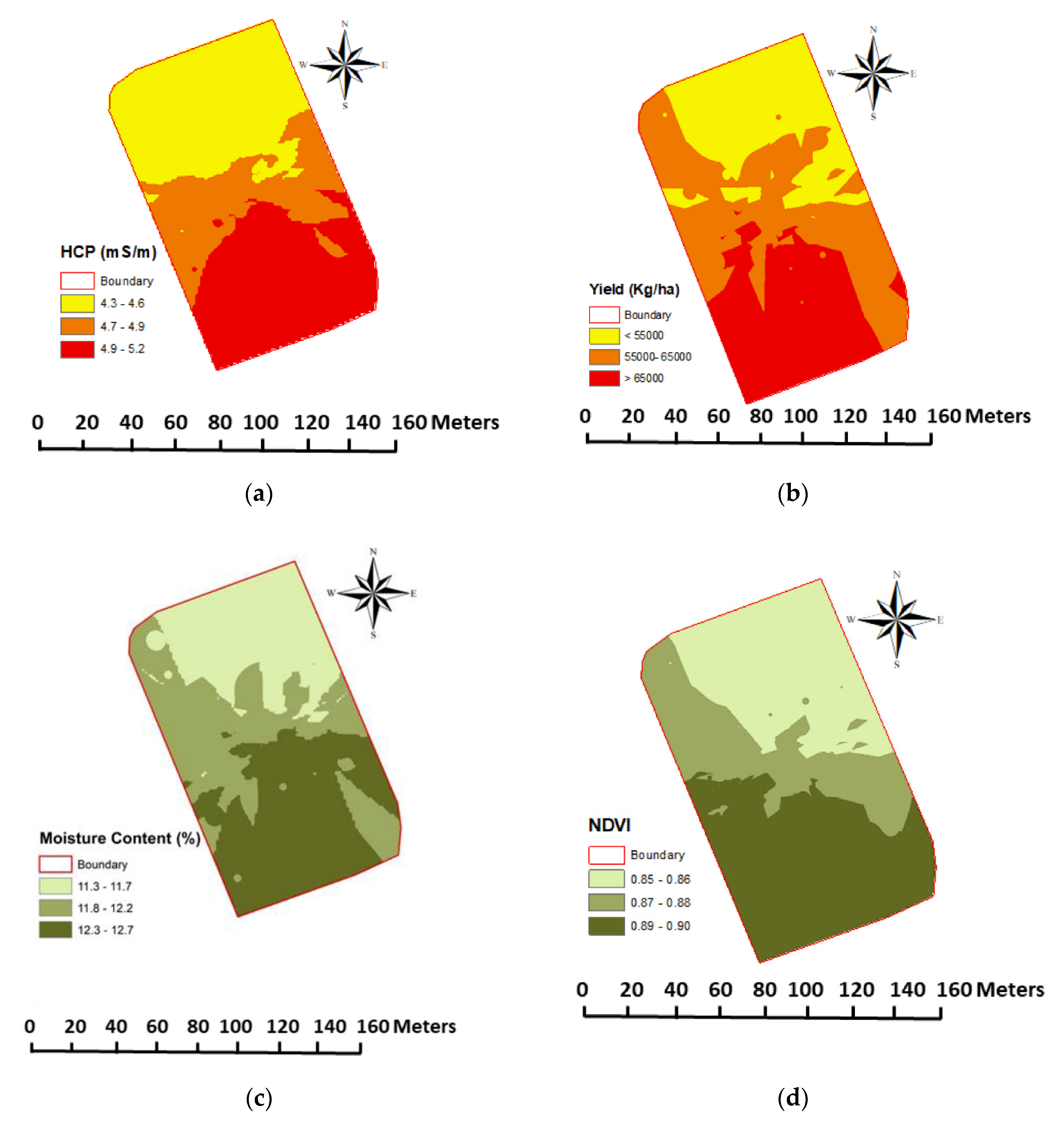
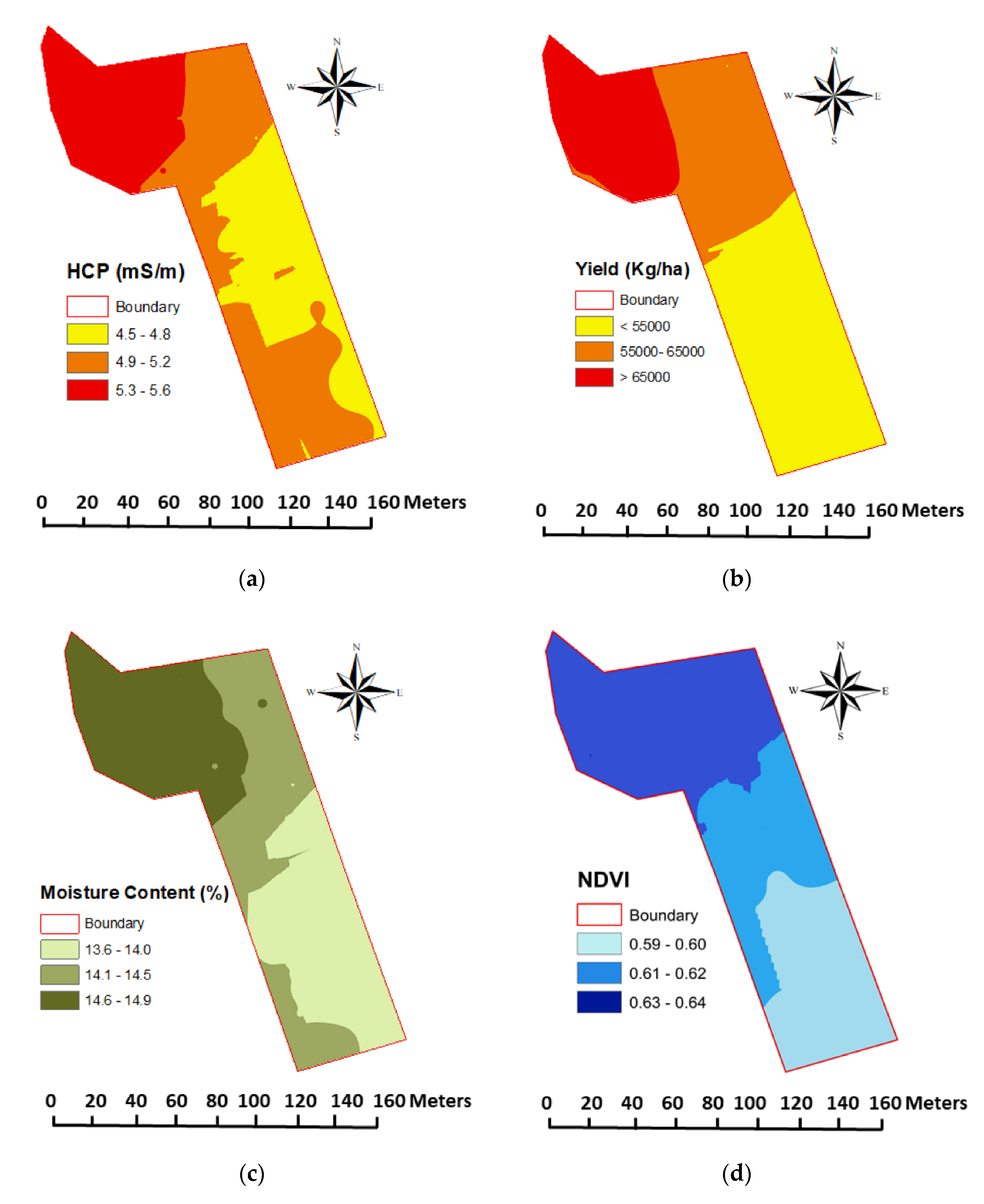
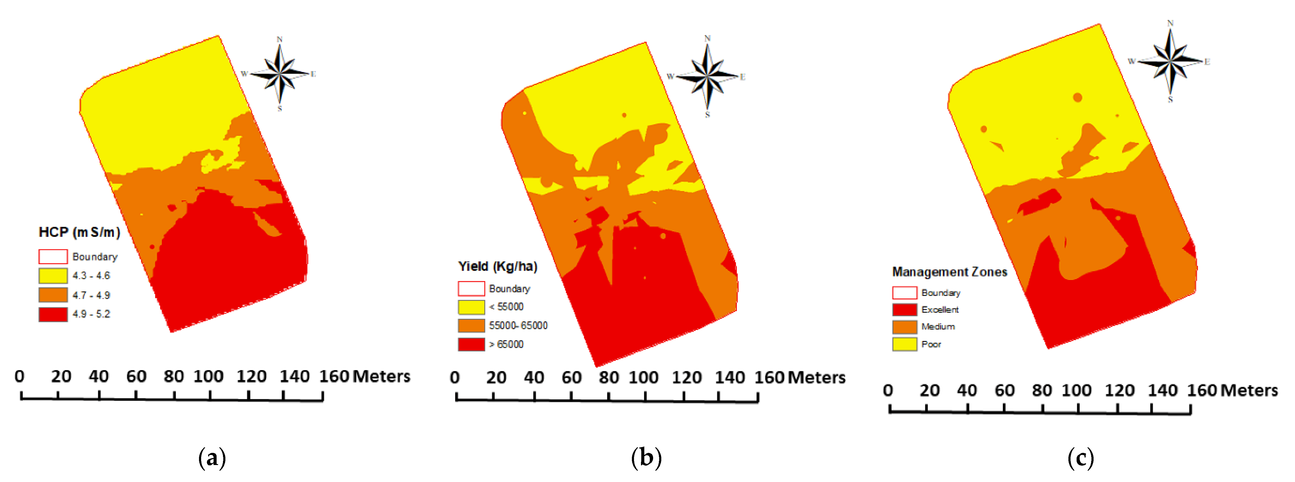
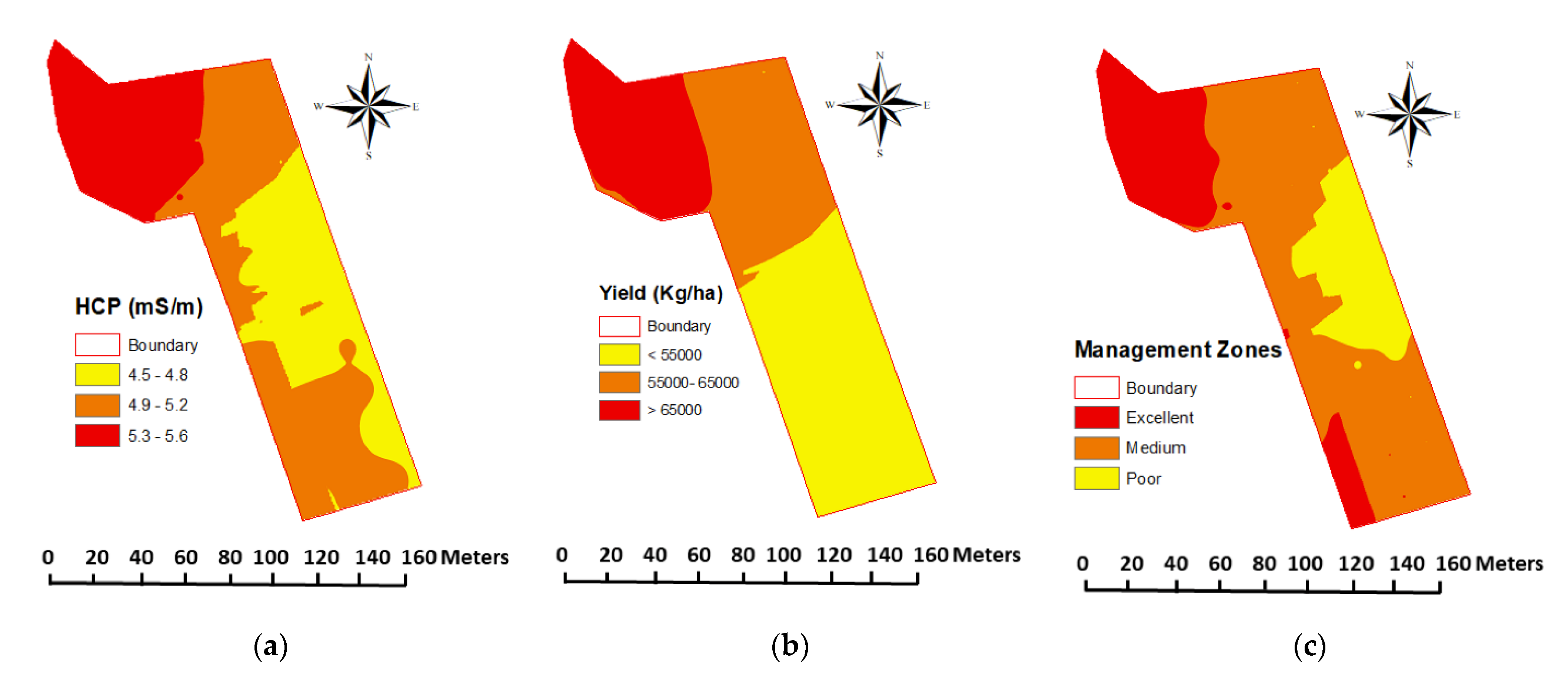
3.4. Interpolation for Within-Field Variability

The GIS interpolated maps of soil and crop properties, produced in ArcGIS using the IDW showed significant spatial variability for the selected properties across Fields 1 and 2 (Figure 2). A higher value of HCP was observed in the southeast part of Field 1, the lower value was observed in the northwest part of this field (Figure 2). A higher value of yield was observed in the south and west parts of the field than those observed in the north and east parts of the field. It was because of high SOM in the southeastern and western parts of the field. Soil organic matter that affects crop productivity has been related with spatial yield variations for effective nutrient management [54,55].
High values of θ were observed in the southwest of the field; whereas, low value was observed in the northeast part. Southwestern parts of the field had the higher NDVI than the northern parts. Yield maps showed substantial spatial variation across the field. High yielding areas were in the southwest of the field, and low yielding areas were in the north of the field in most of the parameters for Field 1. Maps presented in Figure 2 also showed that the tuber yield was higher in the areas with more HCP, θ, and NDVI. The overall results of descriptive statistics and the interpolated maps suggested moderate variability in soil properties and tuber yield within-field, except for HCP, θ, and NDVI, which was highly variable for Field 1.
The maps of Field 2 have been shown in Figure 3. Higher values of HCP, θ, and yield were observed in western parts of the field and lower value of HCP and θ was observed in the east of the field, whereas the lower value of yield was observed in the southeast part of the field. The presence of soil moisture content enhances the crop growth by improving nutrient use efficiency of soils/crops [54,55].
Higher value of NDVI was observed in the northwest parts of the field where lower value of NDVI was observed in the southern part of the field. Maps of Field 2 also showed that tuber yield was higher in the areas with high θ, NDVI, and HCP values.
The MZs maps or the relationships of yield developed with θ, NDVI, and HCP can help growers to manage their practices according to variations in field HCP, θ, and NDVI. The HCP maps of a field may be obtained either commercially or upon request from governments’ agricultural services related ministries. For example, the department of Agriculture and Agri-Food Canada (https://www.agr.gc.ca/eng/?id=1343066456961) provides interactive agriculture-related maps, geospatial data, and tools to help you make better decisions for environmentally responsible yet competitive agriculture. There exist simple methods to measure θ and NDVI using a variety of sensors available in the market. Gozdowski et al. [21] also showed significant variations in NDVI within the MZs. This vegetation index reflects actual crop status, which relates to the soil properties that are important to satisfy crop requirements. Consequently, the NDVI may be a useful tool for MZ delineation, especially because their measurements are simple to make. The moisture content of soil can also be determined by oven dry method. Moreover, the simplest method to determine θ in the soil is “the feel and appearance method”, which is one of several irrigation scheduling methods used worldwide. It is a way of monitoring soil moisture to determine when to irrigate and how much water to apply.

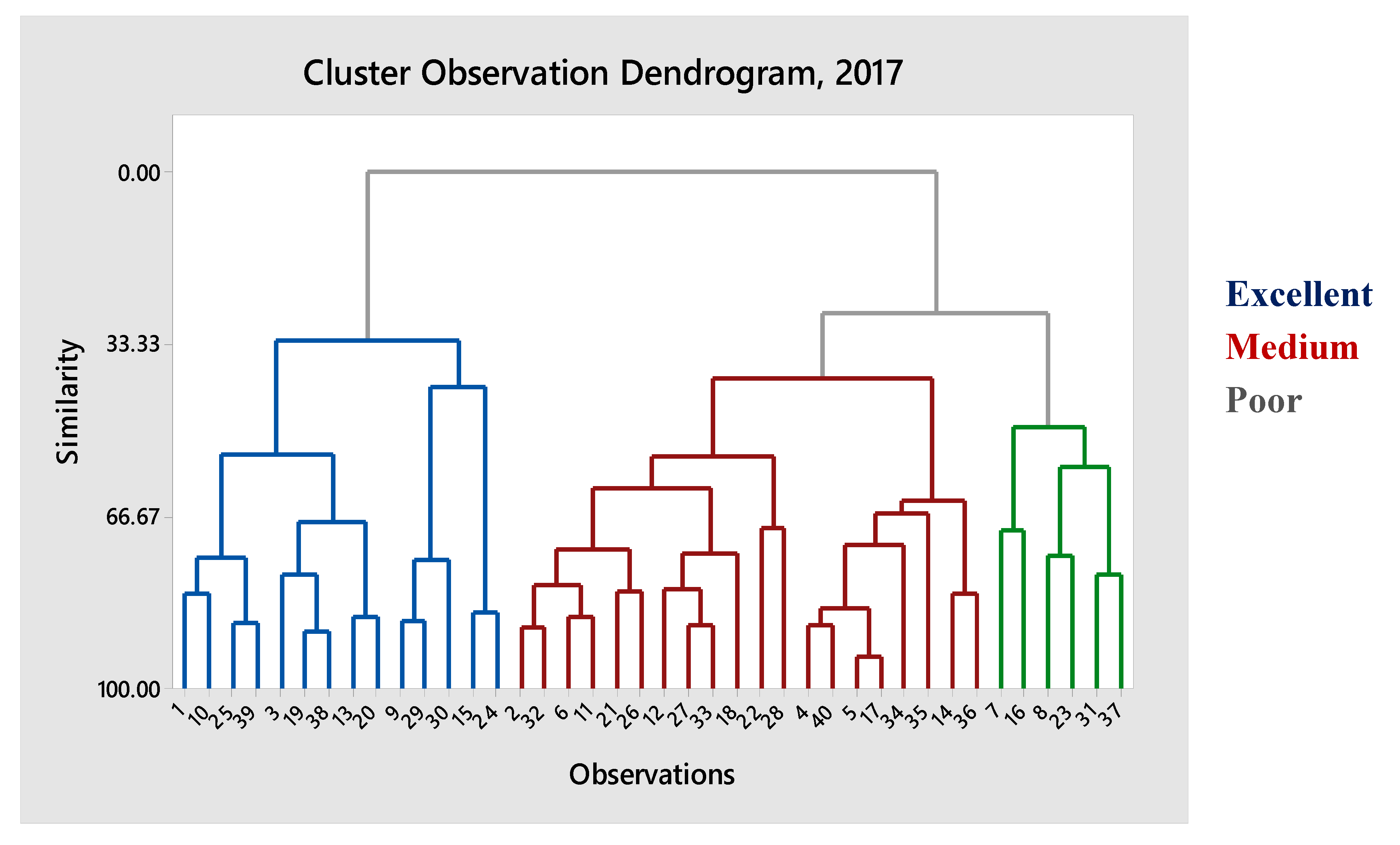
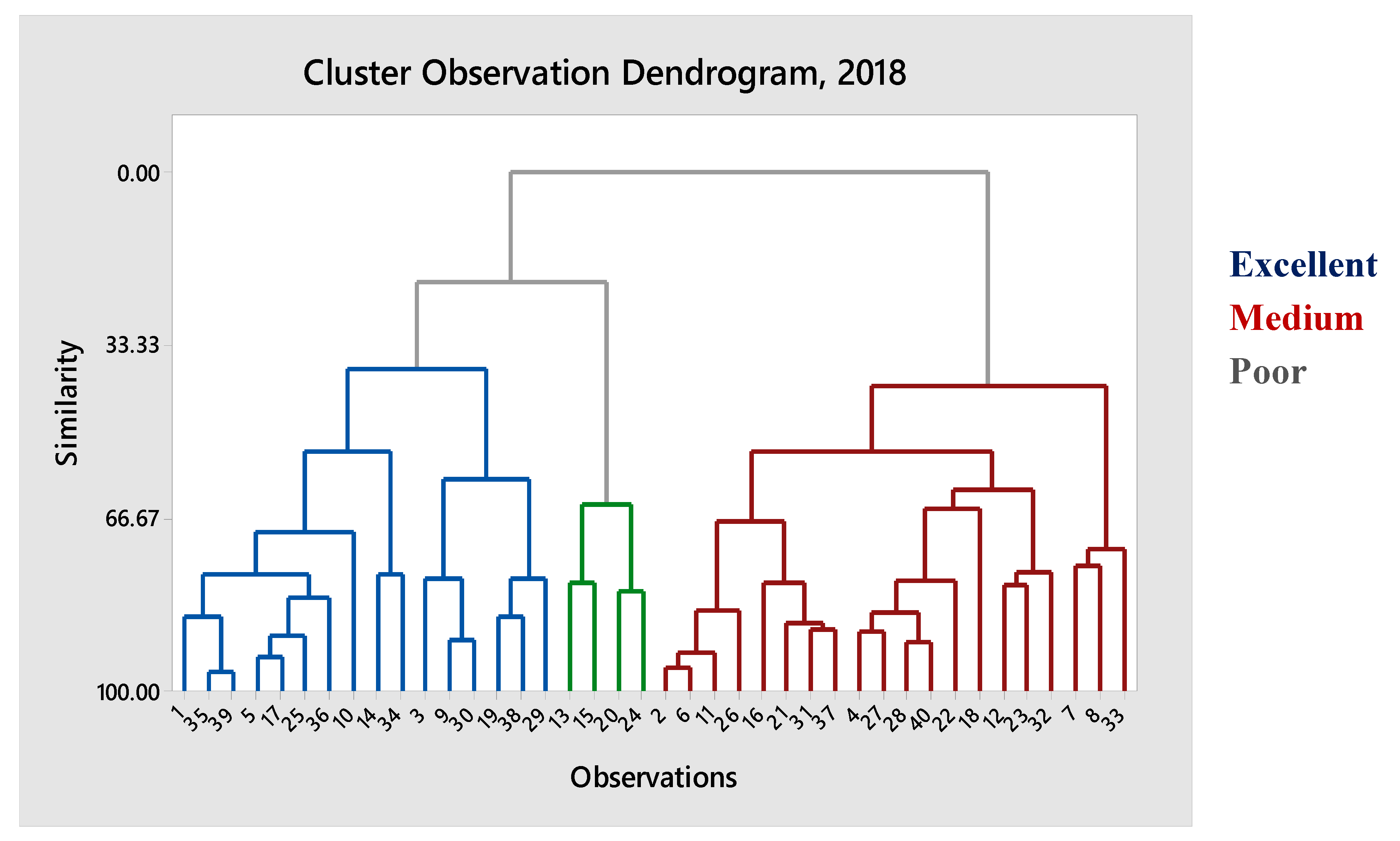
3.5. Cluster Analysis and Management Zones

The results of interpolated maps confirmed that there exists spatial variations in the fields, which require the development of MZs for site-specific nutrient management. Cluster analysis was performed and soil and crop properties were clustered in the form of groups that differentiate the high yielding and low yielding areas of the fields, by separating the high yielding sampling points and low yielding sampling points. The dendrograms of the Fields 1 and 2 are shown in Figure 4 and Figure 5, representing clustered soil and tuber yield data into three groups based on their similarity level. The productivity levels to develop MZs were decided based on tuber yield data, i.e., excellent (yield > 65,000 kg ha−1), medium (yield 55,000–65,000 kg ha−1), poor (yield < 55,000 kg ha−1) for both fields. The grouping of soil and crop properties in dendrogram showed that most of the sampling points fall in medium productivity area (Figure 4 and Figure 5) and a of couple data points fell in excellent productivity area and a very few points lied in the poor productivity area of the field, which indicated that both were high yielding fields. Moreover, the cluster analysis differentiated the high yielding and low yielding areas of the fields.
After cluster analysis, the comparison of mean tuber yield and soil properties for MZs in Field 1 are shown in Table 3. In this, field HCP and yield were significantly different in all zones having the highest values in excellent zones. Highest values were observed for θ and SOM in the medium zone. Lime index and pH had maximum values in the poor zone. Phosphate, K, Fe, and NDVI were not significantly variable in all the zones.
Similarly, in Field 2 (Table 4), HCP, θ, pH, K, and yield were significantly different in all of the zones having the highest values in the excellent zones. Phosphate, Fe, and CEC had higher values in excellent zones; however, their values differ moderately across the field. Soil organic matter and NDVI were the least significant in the field. Since higher values of HCP, θ, pH, K, P, Fe, and CEC determine good soil health for potato production [30,56] their presence in the excellent zone ensures higher tuber yield in excellent zones as compared to the poor and medium zones [29,31]. The tuber yield obtained from Fields 1 and 2 was higher than the country average vales of tuber yield of nations from Europe and America that adopt the best nutrient management practices, as tabulated by Koch et al. [57]. The values of SOM and pH reported in Table 1, Table 3 and Table 4 of this study are in the neighborhood of the values reported by Farooque et al. [31], measured in two potato fields of New Brunswick and two in PEI. Moreover, the values of P and K reported by Zare et al. [56] that resulted in enhanced tuber yield in potato fields of PEI and New Brunswick are in the range of the values of P and K of excellent and medium zones, or high yield producing portions of Fields 1 and 2 of the current study. Stark et al. [58] commended that potatoes have high nutrient demands, as they require approximately 247 kg of N, 33.5 kg of P, and 335 kg of K per hectare to produce approximately 56,491 kg/ha yield of Russet Burbank in southern Idaho, USA.
The clustered data were imported into ArcGIS where MZs were developed indicating the different levels of productivity that required the variable application of nutrients across the fields. The comparison of HCP and yield mapped in MZs for the Fields 1 and 2 are shown in Figure 6 and Figure 7, respectively. The information regarding tuber yield related with MZs is important as a part of a successful agronomic strategy to adequately manage nutrients for potato crop, which is essential throughout the whole growth period [57]. Development of MZs with the help of soil characteristics, especially from the proximal sensing information of soil’s HCP can help farmers manage crop inputs other than nutrients during the whole growth period. The following information generated from MZs can help producers reduce the gap between the actual yield and the yield potential [59]. The results confirm the findings of [26,27] who delineated MZs using EM38 measured soil electrical conductivity, and related it with soil properties used to related MZs and tuber yield. The approach is recommended to have a control on managing within-field variability of soil and crop characteristics for enhancing potato productivity and profitability, while reducing the environmental impacts of agricultural practices.

4. Conclusions

This research revealed that there exists spatial variability within potato fields that require precise agricultural inputs. Geostatistical analysis showed that most of the parameters had strong spatial dependencies, and stepwise regression explained 89 to 90% of within-field variability, while considering all of the studied variables (i.e., HCP, θ, SOM, pH, P, K, Fe, LI, P/Al, CEC, and NDVI), 71 to 86% while considering the most significant variables (i.e., HCP, θ, and NDVI), and 52 to 83% while considering the easily measureable variables (θ and NDVI). The results of cluster analysis and comparison of means of tuber yield with other soil variables suggested that ground conductivity; i.e., HCP, θ, NDVI, and tuber yield data can be utilized to delineate MZs for site-specific nutrient management in potato fields. Field implications of this research include the fact that MZs can provide a better way to manage the spatial variability of soil properties and tuber yield within fields. The use of MZs would decrease the cost of production while increasing farm profitability. However, the farmers may face challenges in determining the recommended soil properties to construct MZ maps. There may exist commercial services for assisting farmers in obtaining maps of variable soil properties of their fields, or such maps may be provided by government departments responsible for guiding farmers to make informed decisions about agricultural management practices. Among various examples related to other countries for this purpose is the example of the department of Agriculture and Agri-Food Canada (https://www.agr.gc.ca/eng/?id=1343066456961) that provides interactive agriculture-related maps, geospatial data, and tools to help you make better decisions for environmentally responsible yet competitive agriculture. For properties, such as θ and NDVI, there exist simple methods and tools of measurements, such as commercially available sensors. The moisture content of soil can also be determined by the oven dry method, or, simply, by the feel and appearance method.

Author Contributions

Conceptualization, H.K. and A.A.F.; methodology, H.K., A.A.F. and B.A.; software, H.K. and F.A.; validation, A.A.F.; formal analysis, H.K. and F.A.; investigation, H.K., A.A.F. and F.A.; resources, A.A.F.; data curation, H.K. and A.A.F.; writing—original draft preparation, H.K. and F.A.; writing—review and editing; A.A.F., B.A., T.J.E. and Q.U.Z.; supervision, A.A.F., B.A. and Q.U.Z.; project administration, A.A.F., B.A., T.J.E. and Q.U.Z.; funding acquisition, A.A.F. All authors have read and agreed to the published version of the manuscript.

Funding

This research was supported by the Natural Science and Engineering Research Council of Canada, Prince Edward Island Potato Board, Canadian Horticultural Council, Potato Board New Brunswick, New Brunswick Department of Agriculture, Aquaculture, and Fisheries (CAP program), and Agriculture and Agri-Food Canada.

Acknowledgments

The authors thank Ryan Barret (Research Coordinator, Prince Edward Island Potato Board), Joe Brennan and Khalil Al-Mughrabi (New Brunswick Potato Transformation Initiative), and the Precision Agriculture Team at the University of Prince Edward Island for their cooperation and assistance during the experiment.

Conflicts of Interest

The authors declare no conflict of interest.

References

  1. Birch, P.R.J.; Bryan, G.; Fenton, B.; Gilroy, E.M.; Hein, I.; Jones, J.T.; Prashar, A.; Taylor, M.A.; Torrance, L.; Toth, I.K. Crops that feed the world 8: Potato: Are the trends of increased global production sustainable? J. Food Secur. 2012, 4, 477–508. [Google Scholar] [CrossRef]
  2. Agriculture and Agri Food Canada (AAFC). Potato Marketing and Cost of Productions. Potato Market Information Review 2016–2017. 2017. Available online: http://www.agr.gc.ca/resources/prod/doc/pdf/potato_market_review_revue_marche_pomme_terre_2017-eng.pdf (accessed on 9 January 2020).
  3. Ziadi, N.; Cambouris, A.N.; Nyiraneza, J.; Nolin, M.C. Across a landscape, soil texture controls the optimum rate of N fertilizer for maize production. Field Crops Res. 2013, 148, 78–85. [Google Scholar] [CrossRef]
  4. Po, E.A.; Snapp, S.S.; Kravchenko, A. Potato yield variability across the landscape. Agron. J. 2010, 102, 885–894. [Google Scholar] [CrossRef]
  5. Starr, G.C.; Rowland, D.; Griffin, T.S.; Olanya, O.M. Soil water in relation to irrigation, water uptake and potato yield in a humid climate. Agric. Water Manag. 2008, 95, 292–300. [Google Scholar] [CrossRef]
  6. Reeves, D.W. The role of soil organic matter in maintaining soil quality in continuous cropping systems. Soil Tillage Res. 1997, 43, 131–167. [Google Scholar] [CrossRef]
  7. Zhang, Q. Precision Agriculture Technology for Crop Farming; Taylor & Francis Group: Prosser, WA, USA, 2016. [Google Scholar]
  8. Antle, J.M.; Basso, B.; Conant, R.T.; Godfray, H.C.J.; Jones, J.W.; Herrero, M.; Howitt, R.E.; Keating, B.A.; Munoz-Carpena, R.; Rosenzweig, C.; et al. Towards a new generation of agricultural system data, models and knowledge products: Design and improvement. Agric. Syst. 2017, 155, 255–268. [Google Scholar] [CrossRef]
  9. Baret, F.; Houles, V.; Guérif, M. Quantification of plant stress using remote sensing observations and crop models: The case of nitrogen management. J. Exp. Bot. 2007, 58, 869–880. [Google Scholar] [CrossRef] [Green Version]
  10. Foley, J.A.; Ramankutty, N.; Brauman, K.A.; Cassidy, E.S.; Gerber, J.S.; Johnston, M.; Mueller, N.D.; O’Connell, C.; Ray, D.K.; West, P.C.; et al. Solutions for a cultivated planet. Nature 2011, 478, 337–342. [Google Scholar] [CrossRef] [Green Version]
  11. Sánchez, P.A. Tripling crop yields in tropical Africa. Nat. Geosci. 2010, 3, 299–300. [Google Scholar] [CrossRef]
  12. Slingo, J.M.; Challinor, A.J.; Hoskins, B.J.; Wheeler, T.R. Introduction: Food crops in a changing climate. Philos. Trans. R. Soc. B Biol. Sci. 2005, 360, 1983–1989. [Google Scholar] [CrossRef] [Green Version]
  13. Mann, K.K.; Schumann, A.W.; Obreza, T.A.; Harris, W.G.; Shukla, S. Spatial variability of soil physical properties affecting Florida citrus production. Soil Sci. 2010, 175, 487–499. [Google Scholar] [CrossRef]
  14. Brogi, C.; Huisman, J.A.; Herbst, M.; Weihermüller, L.; Klosterhalfen, A.; Montzka, C.; Reichenau, T.G.; Vereecken, H. Simulation of spatial variability in crop leaf area index and yield using agroecosystem modeling and geophysics-based quantitative soil information. Vadose Zone J. 2020, 19, e20009. [Google Scholar] [CrossRef] [Green Version]
  15. Schumann, A.W.; Miller, W.M.; Zaman, Q.U.; Hostler, K.; Buchanon, S.; Cugati, S. Variable rate granular fertilization of citrus groves: Spreader performance with single-tree prescription zones. Appl. Eng. Agric. 2006, 22, 19–24. [Google Scholar] [CrossRef]
  16. Ferguson, R.B.; Lark, R.M.; Slater, G.P. Approaches to management zone definition for use of nitrification inhibitors. Soil Sci. Soc. Am. J. 2003, 67, 937–947. [Google Scholar] [CrossRef]
  17. Zhang, C.; Walters, D.; Kovacs, J.M. Applications of low altitude remote sensing in agriculture upon farmers’ requests—A case study in northeastern Ontario, Canada. PLoS ONE 2014, 9, e112894. [Google Scholar] [CrossRef]
  18. Yasrebi, J.; Saffari, M.; HamedFathi, N.; Emadi, M.; Baghernejad, M. Spatial variability of soil fertility properties for precision agriculture in southern Iran. J. Appl. Sci. 2008, 8, 1642–1650. [Google Scholar] [CrossRef]
  19. Lindblom, J.; Lundström, C.; Ljung, M.; Jonsson, A. Promoting sustainable intensification in precision agriculture: Review of decision support systems development and strategies. Precis. Agric. 2017, 18, 309–331. [Google Scholar] [CrossRef] [Green Version]
  20. Elstein, D. Management zones help in precision agriculture. Agric. Res. 2003, 51, 17. [Google Scholar]
  21. Gozdowski, D.; Stepien, M.; Samborski, S.S.; Dobers, E.S.; Szatylowicz, J.; Chormanski, J. Determination of the most relevant soil properties for the delineation of management zones in production fields. Commun. Soil Sci. Plant Anal. 2014, 45, 2289–2304. [Google Scholar] [CrossRef]
  22. Abbas, F.; Afzaal, H.; Farooque, A.A.; Tang, S. Crop Yield Prediction through Proximal Sensing and Machine Learning Algorithms. Agron. J. 2020, 10, 1046. [Google Scholar]
  23. Kitchen, N.R.; Sudduth, K.A.; Myers, D.B.; Drummond, S.T.; Hong, S.Y. Delineating productivity zones on claypan soil fields using apparent soil electrical conductivity. Comput. Electron. Agric. 2005, 46, 285–308. [Google Scholar] [CrossRef]
  24. Yari, A.; Madramootoo, C.A.; Woods, S.A.; Adamchuk, V.I.; Huang, H.H. Assessment of field spatial and temporal variabilities to delineate site-specific management zones for variable-rate irrigation. J. Irrig. Drain. Eng. 2017, 143, 04017037. [Google Scholar] [CrossRef]
  25. Kaufman, L.; Rousseeuw, P.J. Finding Groups in Data: An Introduction to Cluster Analysis; John Wiley & Sons: New York, NY, USA, 1990. [Google Scholar]
  26. Cambouris, A.N.; Nolin, M.C.; Zebarth, B.J.; Laverdière, M.R. Soil management zones delineated by electrical conductivity to characterize spatial and temporal variations in potato yield and in soil properties. Am. J. Potato Res. 2006, 83, 381–395. [Google Scholar] [CrossRef]
  27. Cambouris, A.N.; Zebarth, B.J.; Ziadi, N.; Perron, I. Precision agriculture in potato production. Potato Res. 2014, 57, 249–262. [Google Scholar] [CrossRef]
  28. Khan, H.; Acharya, B.; Farooque, A.A.; Abbas, F.; Zaman, Q.; Esau, T.J. Soil and crop variability induced management zones to optimize potato tuber yield. Appl. Eng. Agric. 2020, 36, 499–510. [Google Scholar] [CrossRef]
  29. Farooque, A.A.; Zare, M.; Abbas, F.; Bos, M.; Esau, T.; Zaman, Q. Forecasting potato tuber yield using soil electromagnetic induction. Eur. J. Soil Sci. 2019. [Google Scholar] [CrossRef]
  30. Tang, S.; Farooque, A.A.; Bos, M.; Abbas, F. Modelling DUALEM-2 measured soil conductivity as a function of measuring depth to correlate with soil moisture content and potato tuber yield. Precis. Agric. 2019, 21, 484–502. [Google Scholar] [CrossRef]
  31. Farooque, A.A.; Zare, M.; Abbas, F.; Zaman, Q.; Bos, M.; Esau, T.; Acharya, B.; Schumann, A.W. Evaluation of DualEM-II sensor for soil moisture content estimation in the potato fields of Atlantic Canada. Plant Soil Environ. 2019, 65, 290–297. [Google Scholar] [CrossRef] [Green Version]
  32. Kerry, R.; Oliver, M.A. Variograms of ancillary data to aid sampling for soil surveys. Precis. Agric. 2003, 4, 261–278. [Google Scholar] [CrossRef]
  33. Angers, D.A.; Edward, L.M.; Sanderson, J.B.; Bissonnette, N. Soil organic matter quality and aggregate stability under eight potato cropping sequences in a fine sandy loam of Prince Edward Island. Can. J. Soil Sci. 1999, 79, 411–417. [Google Scholar] [CrossRef]
  34. Bowman, R.A.; Olsen, S.R.; Watanabe, F.S. Greenhouse evaluation of residual phosphate by four phosphorus methods in neutral and calcareous soils. Soil Sci. Soc. Am. J. 1978, 42, 451–454. [Google Scholar] [CrossRef]
  35. Mayer, K.D.; Starkey, B.J. Simpler flame photometric determination of erythrocyte sodium and potassium: The reference range for apparently healthy adults. Clin. Chem. 1977, 23, 275–278. [Google Scholar] [CrossRef] [PubMed]
  36. Wilson, A.D. The micro-determination of ferrous iron in silicate minerals by a volumetric and a colorimetric method. Analyst 1960, 85, 823–827. [Google Scholar] [CrossRef]
  37. Hendershot, W.H.; Duquette, M. A simple barium chloride method for determining cation exchange capacity and exchangeable cations. Soil Sci. Soc. Am. J. 1986, 50, 605–608. [Google Scholar] [CrossRef]
  38. Brown, J.R.; Cisco, J.R. An improved Woodruff buffer for estimation of lime requirements. Soil Sci. Soc. Am. J. 1984, 48, 587–592. [Google Scholar] [CrossRef]
  39. Konen, M.E.; Jacobs, P.M.; Burras, C.L.; Brandi, J.T.; Joseph, A.M. Equations for Predicting Soil Organic Carbon Using Loss-on-Ignition for North Central U.S. Soils. Soil Sci. Soc. Am. J. 2002, 66, 1878–1881. [Google Scholar] [CrossRef]
  40. Schulte, E.E.; Hopkins, B.G. Estimation of Soil Organic Matter by Weight Loss-On-Ignition. Soil Org. Matter Anal. Interpret. 1996, 46, 21–31. [Google Scholar]
  41. Navarro, A.F.; Cegarra, J.; Roig, A.; Garcia, D. Relationships between organic matter and carbon contents of organic wastes. Bioresour. Technol. 1993, 44, 203–207. [Google Scholar] [CrossRef]
  42. Getting Started with Minitab 18. 2017. Available online: www.minitab.com (accessed on 24 November 2020).
  43. Wilding, L. Spatial variability: Its documentation, accommodation and implication to soil surveys. In Soil Spatial Variability, Proceedings of the Workshop of ISSS and SSA Las Vegas, Las Vegas, NV, USA, 30 November–1 December 1984; Nielsen, D.R., Bouma, J., Eds.; Centre for Agricultural Publishing and Documentation, Pudoc: Wageningen, The Netherlands, 1985; pp. 166–189. [Google Scholar]
  44. Robertson, G.P. GS+: Geostatistics for the Environmental Sciences; Gamma Design Software: Plainwell, MI, USA, 2008. [Google Scholar]
  45. Bronowicka-Mielniczuk, U.; Mielniczuk, J.; Obroślak, R.; Wojciech, P. A Comparison of Some Interpolation Techniques for Determining Spatial Distribution of Nitrogen Compounds in Groundwater. Int. J. Environ. Res. 2019, 13, 679–687. [Google Scholar] [CrossRef] [Green Version]
  46. Webster, R.; Oliver, M. Geostatistics for Environmental Scientists; John Wiley & Sons: New York, NY, USA, 2007. [Google Scholar]
  47. Zhu, X. GIS for Environmental Applications: A Practical Approach; Routledge: Abingdon, UK, 2016. [Google Scholar]
  48. Li, J. Assessing spatial predictive models in the environmental sciences: Accuracy measures, data variation and variance explained. Environ. Model. Softw. 2016, 80, 1–8. [Google Scholar] [CrossRef]
  49. Barrett, R. Nutrient Management in PEI Potato Production—Key Points to Consider When Making Fertility Program Decisions on Your Farm. Factsheet Worksheet and Factsheet. 2018. Available online: http://peipotatoagronomy.com/wp-content/uploads/2018/01/Nutrient-Mgmt-Factsheet-Jan17.pdf (accessed on 24 November 2020).
  50. USDA-NRCS. Soil Electrical Conductivity. Soil Quality Kit—Guide for Educators. 2019. Available online: https://www.nrcs.usda.gov/Internet/FSE_DOCUMENTS/nrcs142p2_053280.pdf (accessed on 24 November 2020).
  51. Redulla, C.A.; Davenport, J.R.; Evans, R.G.; Hattendorf, M.J.; Alva, A.K.; Boydston, R.A. Relating potato yield and quality to field scale variability in soil characteristics. Am. Potato J. 2002, 79, 317–323. [Google Scholar] [CrossRef]
  52. Waterer, D. Impact of high soil pH on potato yields and grade losses to common scab. Can. J. Plant Sci. 2002, 82, 583–586. [Google Scholar] [CrossRef] [Green Version]
  53. Dorff, E.; Beaulieu, M.S. Canadian Agriculture at a Glance—Feeding the Soil Puts Food on Your Plate. Analytical Paper, Agriculture Division. 2011. Catalogue No. 96 325 X—No. 004 ISSN 0-662-35659-4. Available online: https://www150.statcan.gc.ca/n1/en/pub/96-325-x/2014001/article/13006-eng.pdf?st=gjGjkUaI (accessed on 24 November 2020).
  54. Machado, F.C.; Montanari, R.; Shiratsuchi, L.S.; Lovera, L.H.; Lima, E.D.S. Spatial dependence of electrical conductivity and chemical properties of the soil by electromagnetic induction. Revista Brasileira de Ciência do Solo 2015, 39, 1112–1120. [Google Scholar] [CrossRef] [Green Version]
  55. Machado, P.L.O.; Bernardi, A.C.D.C.; Valencia, L.I.O.; Molin, J.P.; Gimenez, L.M.; Silva, C.A.; Andrade, A.G.D.; Madari, B.E.; Meirelles, M.S.P. Mapeamento da condutividade elétrica e relação com a argila de Latossolo sob plantio direto. Pesquisa Agropecuária Brasileira 2006, 41, 1023–1031. [Google Scholar] [CrossRef] [Green Version]
  56. Zare, M.; Farooque, A.A.; Abbas, F.; Zaman, Q.U.; Bos, M. Trends in the variability of potato tuber yield under selected land and soil characteristics. Plant Soil Environ. 2019, 65, 111–117. [Google Scholar] [CrossRef] [Green Version]
  57. Koch, M.; Naumann, M.; Pawelzik, E.; Gransee, A.; Thiel, H. The Importance of Nutrient Management for Potato Production Part I: Plant Nutrition and Yield. Potato Res. 2020, 63, 97–119. [Google Scholar] [CrossRef] [Green Version]
  58. Stark, J.C.; Westermann, D.T.; Hopkins, B. Nutrient Management Guidelines for Russet Burbank Potatoes; University of Idaho, College of Agricultural and Life Sciences: Moscow, ID, USA, 2004. [Google Scholar]
  59. Michel, A.; Sinton, S.M.; Falloon, R.E.; Shah, F.A.; Dellow, S.J.; Pethybridge, S.J. Biotic and abiotic factors affecting potato yields in Canterbury, New Zealand. In Proceedings of the 17th ASA Conference, Hobart, Australia, 20–24 September 2015; pp. 211–214. [Google Scholar]
Figure 1. Layouts of fields of Prince Edward Island showing the grid nodes inside the fields having sampling points as n = 40; 25 × 25 m for Field 1 (a) and n = 39; 25 × 25 m for Field 2 (b).
Agronomy 10 01854 g001
Figure 2. Interpolated maps of soil properties and crop yield for the Field 1. (a) Horizontal coplanar geometry (HCP), (b) yield, (c) moisture content (θ), (d) normalized difference vegetation index (NDVI).
Agronomy 10 01854 g002
Figure 3. Interpolated maps of soil properties and crop yield for the Field 2. (a) Horizontal coplanar geometry (HCP), (b) yield, (c) moisture content (θ), (d) normalized difference vegetation index (NDVI).
Agronomy 10 01854 g003
Figure 4. Observation dendrogram of soil properties and tuber yield for Field 1.
Agronomy 10 01854 g004
Figure 5. Observation dendrogram of soil properties and tuber yield for Field 2.
Agronomy 10 01854 g005
Figure 6. Comparison of delineated management zones for Fields 1: (a) HCP, (b) tuber yield, and (c) management zones.
Agronomy 10 01854 g006
Figure 7. Comparison of delineated management zones for Field 2: (a) HCP, (b) tuber yield, and (c) management zones.
Agronomy 10 01854 g007
Table 1. Results of descriptive statistics for soil and crop properties of Fields 1 and 2.
Fields and SamplingVariableMeanMinMaxCV (%)
Date
Field 1; 8 June 2017HCP (mS m−1)7.304.1010.928.8
θ (%)16.18.9023.626.3
SOM (%)2.422.002.9012.1
pH5.625.206.003.09
P (mg kg−1)35123658929.8
K (mg kg−1)17310927320.1
Fe (mg kg−1)27421640111.7
LI6.966.807.101.06
CEC (Meq 100 g−1)5.134.007.0014.1
Field 1; 13 July 2017HCP (mS m−1)4.761.728.3243.3
θ (%)12.04.9219.634.5
SOM (%)2.452.003.2012.4
pH5.314.806.004.16
P (mg kg−1)47631481228.8
K (mg kg−1)22211847137.3
Fe (mg kg−1)3172634209.72
LI6.586.306.801.68
CEC (Meq 100 g−1)10.08.0013.010.5
NDVI 0.880.730.957.63
Yield * (kg)14.410.118.217.1
Field 2; 11 June 2018HCP (mS m−1)5.282.508.2028.0
θ (%)8.216.1011.115.1
SOM (%)2.590.503.1015.8
pH5.615.206.204.11
P (mg kg−1)41026567024.9
K (mg kg−1)16910126022.9
Fe (mg kg−1)2932323419.52
LI6.686.507.001.95
CEC (Meq 100 g−1)8.284.0010.015.9
Field 2; 10 July 2018HCP (mS m−1)6.874.109.8016.8
θ (%)14.38.9019.017.4
SOM (%)2.572.303.106.83
pH5.364.506.105.32
P (mg kg−1)39729249812.6
K (mg kg−1)20110125415.6
Fe (mg kg−1)26015035012.1
LI6.706.406.901.55
CEC (Meq 100 g−1)8.445.0011.014.6
NDVI 0.620.410.7916.2
Yield * (kg)16.19.0023.216.6
CV = coefficient of variation, Min = minimum, Max = maximum, HCP = horizontal coplanar geometry, θ = moisture content, SOM = soil organic matter, P = phosphorous, K = potash, Fe = iron, LI = lime index, CEC = cation exchange capacity, NDVI = normalized difference vegetation index. * Yield was collected at the time of harvesting on 2 October 2017 (Field 1) and 4 October 2018 (Field 2).
Table 2. Semivariogram models for spatial dependencies of soil parameters of Fields 1 and 2.
Sampling DateVariableNuggetSillRangeR2RSSModel
Field 1; 13 July 2017HCP (mS m−1)0.002.0134.30.900.36Gaussian
θ (%)0.019.3627.50.980.73Gaussian
SOM (%)0.000.0523.90.917.43 × 10–5Gaussian
pH0.000.4433.70.880.02Gaussian
P (mg kg−1)10.0550520.90.988,184,600Gaussian
K (mg kg−1)1.00160823.30.8967,185Gaussian
Fe (mg kg−1)1.00226430.20.85480,573Gaussian
LI0.000.6234.80.870.04Gaussian
CEC (Meq 100−1)1.501.5065.80.280.37Linear
NDVI0.000.0233.00.857.16 × 10–5Gaussian
Yield *0.0111.930.90.908.75Gaussian
Field 2; 10 July 2018HCP (mS m−1)0.001.7219.00.000.13Spherical
θ (%)3.317.7892.10.740.44Exponential
SOM (%)0.000.0325.10.787.86 × 10–5Gaussian
pH0.160.1665.80.360.08Linear
P (mg kg−1)2612261265.80.422,575,025Linear
K (mg kg−1)1055105565.80.07118,162Linear
Fe (mg kg−1)1.00107929.20.78213,822Gaussian
LI0.010.0165.80.318.68 × 10–5Linear
CEC (Meq 100−1)1.501.5065.80.280.37Linear
NDVI0.000.0143.41.002.60× 10–9Spherical
Yield *7.257.2565.80.0018.1Linear
Abbreviations, symbols, and harvesting dates are given in the footnotes section of Table 1.
Table 3. Comparison of mean tuber yield and soil properties for management zones for Field 1.
Soil PropertiesZone 1Zone 2Zone 3
ExcellentMediumPoor
Yield > 65,000 (kg ha−1)Yield 55,000–65,000 (kg ha−1)Yield < 55,000 (kg ha−1)
HCP (mS m−1)7.10 a5.58 b4.46 c
θ (%)8.30 ab8.50 a7.39 b
SOM (%)2.50 b2.66 a2.60 a
pH5.40 ab5.55 b5.75 a
P (mg kg−1)306 a415 a407 a
K (mg kg−1)169 a176 a152 a
Fe (mg kg−1)264 a300 a279 a
LI6.60 ab6.62 b6.80 a
CEC (Meq 100g−1)9.00 ab8.76 a7.16 b
NDVI0.70 a0.52 a0.40 a
Yield (kg ha−1)66,736 ab60,034 a51,651 b
Means followed by different letters are significantly different from each other.
Table 4. Comparison of mean tuber yield and soil properties for management zones for Field 2.
Soil PropertiesZone 1Zone 2Zone 3
Excellent MediumPoor
Yield > 65,000 (kg ha−1)Yield 55,000–65,000 (kg ha−1)Yield < 55,000 (kg ha−1)
HCP (mS m−1)9.23 a6.74 b4.10 c
θ (%)18.3 a14.0 b8.90 c
SOM (%)2.53 a2.56 a2.60 a
pH5.86 a5.34 b4.50 c
P (mg kg−1)484 a390 b350 b
K (mg kg−1)244 a200 b101 c
Fe (mg kg−1)284 a260 a150 b
LI6.50 b6.71 a6.70 ab
CEC (Meq 100−1)10.3 a8.28 b8.00 ab
NDVI0.71 a0.61 a0.45 a
Yield (kg ha−1)82,164 a56,247 b32,291 c
Means followed by different letters are significantly different from each other.
Publisher’s Note: MDPI stays neutral with regard to jurisdictional claims in published maps and institutional affiliations.

