Longitudinal variability of thermospheric zonal winds near dawn and dusk

1 Introduction

Thermospheric neutral winds present a highly dynamic behavior with changing geophysical conditions. Understanding their variability becomes critical, as they transfer energy and momentum in the upper atmosphere and directly or indirectly affect the dynamics, morphology and composition of the ionosphere, which can disrupt radiocommunication and navigation systems (e.g., Wang et al., 2021).

Waves present in the thermosphere play a particular role and add significant variability in the wind system. Generally, these waves are classified as (i) planetary waves, which are global in scale with periods of up to several days to a month (Forbes, 1996); (ii) tides, which are also global in scale but with periods that are sub-harmonics of solar and lunar days (Oberheide et al., 2015); and (iii) gravity waves, which are medium-to small-scale oscillations with periods ranging from a few minutes to several hours (Fritts and Alexander, 2003).

Migrating and non-migrating tides originating from the lower atmosphere are recognized as important players in the vertical coupling between the lower and upper atmosphere. The general morphology of these tides has been studied extensively over the past decades (e.g., Lindzen, 1981; Teitelbaum and Vial, 1981; Miyahara et al., 1993; Liu et al., 2010; Forbes et al., 2017) and can be observed as global oscillations in winds, density, temperature and other atmospheric fields. In general, they transfer energy and momentum from the lower regions of the atmosphere into the upper atmosphere and generate longitudinal variations in the various atmospheric state parameters and can modify the global ionosphere-thermosphere (I-T) system (e.g., Immel et al., 2006; Forbes, 2007). Therefore, it is important to understand the spatial and temporal variability they generate in the upper atmosphere.

Thermospheric data derived from satellite accelerometers (e.g., Bruinsma and Biancale, 2003; Sutton et al., 2007; Doornbos et al., 2010) has been used to study global longitudinal structures produced by non-migrating tides. For example, Forbes et al. (2012) used densities from the SETA, CHAMP and GRACE satellites to investigate vertical tidal propagation and to identify the tidal oscillations in the longitudinal structures present in the data; Häusler and Lühr (2009) investigated the non-migrating tidal spectra in zonal wind data at equatorial latitudes obtained from the CHAMP accelerometer with an emphasis on the annual variation of the wave-4 structure at 400 km altitude; Lieberman et al. (2013a) investigated tidal variations in longitudinally averaged CHAMP global zonal winds; Gasperini et al. (2015) used GOCE neutral densities and zonal winds and TIMED-SABER temperatures to study vertical coupling in the thermosphere; Liu et al. (2016) found the presence of wind jets aligned with the magnetic equator in GOCE zonal winds; Dhadly et al. (2020) studied the latitudinal variation in intra-annual oscillations in the GOCE cross-track neutral winds.

This study focuses on longitudinal structures present in zonal winds produced by non-migrating atmospheric tides and observed by the GOCE satellite during dawn and dusk. The year-to-year progression during December solstice is investigated and the contributions from zonal wave-1 to wave-5 structures is studied. The GOCE results are compared to the Climatological Tidal Model of the Thermosphere (CTMT) (Oberheide et al., 2011).

Throughout this paper, the standard nomenclature for tides is used; DEs (DWs) is an eastward (westward) propagating diurnal tide with zonal wavenumber s. For semidiurnal tides, an S is used in place of the D.

This paper is organized in the following manner. Section 2 describes the data used in the study, while Section 3 describes the methodology. In Section 4 the combined contributions of zonal wave-1 to wave-5 structures are presented, and their individual contributions are shown in Section 5. In Section 6, the GOCE results are compared to the CTMT model. Finally, Section 7 provides a summary and discussion of the results.

2 GOCE data

The Gravity field and steady-state Ocean Circulation Explorer (GOCE) satellite was launched on 17 March 2009 into a dawn-dusk Sun-synchronous orbit with an inclination of 96.7° (near-polar orbit) and an altitude of ∼260 km. Its main objective was to study Earth’s gravity field, with thermospheric densities and winds calculated later combining accelerometer and ion thruster data, together with GPS tracking and star camera data. For a description of the determination algorithm see Doornbos et al., 2010. The data set version 2.0 was used for this study, which had been reprocessed with a new implementation of the algorithms (Visser et al., 2019). The algorithm uses a new satellite geometry and aerodynamic model representation (March et al., 2019a), with a new setting of the aerodynamic energy accommodation coefficient (March et al., 2019b).

Even though the GOCE satellite altitude is on the average ∼260 km, it varies with time, starting initially at ∼270 km in 2009 and decreasing to ∼250 km in 2013. The local time corresponding to dawn and dusk also varies. In 2009 the local solar time at the equator crossing for dusk is ∼18 h and by the end of the mission it reaches ∼19 h.

The errors in the GOCE zonal wind are of the order of ∼10%–20%, with the dominant source of errors being biases due to instrument calibration and external models used in the calculation of the winds (Doornbos et al., 2010). In this work, the errors will be attenuated by using residuals, which account for these biases.

Due to the availability of geomagnetically quiet-time data, the December solstice was selected to study the year-to-year progression of the longitudinal variability in the GOCE zonal winds. In order to calculate the perturbations in the GOCE zonal wind measurements, a 27-day window of data was selected for each year; this helps to minimize the effect of the Sun’s rotation. These selected windows are centered as close as possible to the December solstice for the years 2009, 2010, 2011, and 2012, taking into account gaps in the data and geomagnetically active periods. For reference, figures for June 2010 and 2011 are also included in the Supplementary Material. The selected windows are:

• December solstice 2009: 12 December 2009 to 07 January 2010

• December solstice 2010: 05 December 2010 to 31 December 2010

• December solstice 2011: 08 December 2011 to 03 January 2012

• December solstice 2012: 08 December 2012 to 03 January 2013

• June 2010: 04 June 2010 to 30 June 2010 (in Supplementary Material)

• June 2011: 08 June 2011 to 04 July 2011 (in Supplementary Material)

Figure 1A shows the daily F10.7 cm radio flux for the duration of the GOCE wind data set. The periods selected are indicated by green (December solstices) and purple (June solstices) vertical bars. The average F10.7 value for the selected window in December 2009 was 76 sfu. For 2010 that value was 81 sfu. The averages for 2011 and 2012 were higher, at 132 sfu and 109 sfu respectively. The mean F10.7 value for June 2010 was 75 sfu and for June 2011 it was 95 sfu. The geomagnetic activity in these periods was, in general, very low. The average Kp values did not exceed 1⁰ during the December solstice windows and it was below 2⁻ for the June periods. With the exception of one day in December 2011, the daily Kp index is always below a value of 3 for all of the December periods, and reaches 3.3 once during each of the selected June periods. The reason for not including June 2012 and June 2013 in our analysis is due to data gaps and the presence of geomagnetic storms during these periods which precluded us from finding suitable 27-day windows. Figure 1B shows, for the same period as above, the Oceanic Niño Index (ONI), a 3-month running mean of sea-surface temperature anomalies (Bamston et al., 1997) with respect to the mean from 1971 to 2000 in the region 120 to 170°W and 5°N to 5°S. The ONI is used to classify El Niño Southern Oscillation (ENSO). El Niño conditions are present when ONI exceeds +0.5K for 5 consecutive months whereas La Niña conditions correspond to values of ONI of −0.5K or lower. ENSO is categorized into weak (ONI values of 0.5–0.9), moderate (ONI 1.0-1.4), strong (ONI 1.5-1.9) and extreme (values of ONI 2 or higher). Figure 1C shows the Quasi Biennial Oscillation (QBO) U30 index, which corresponds to the zonally averaged wind at 30 hPa over the Equator. It is observed that throughout the span of the GOCE thermospheric data set both of these indices exhibit strong variations which will be discussed in Section 7.

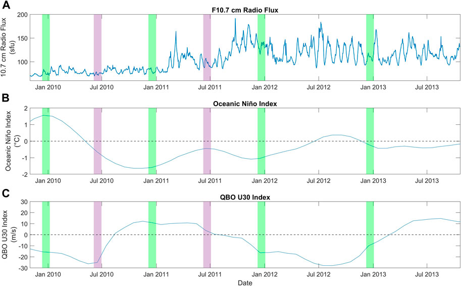
FIGURE 1. F10.7 cm radio flux (A), Oceanic Niño Index (ONI) (B) and Quasi-Biennial Oscillation at 30 hPa (QBO U30) index (C), during the span of the GOCE thermospheric data set. The ONI and QBO indices are 3-month averages plotted at the mid-point of each period. The December and June solstice periods selected are indicated with green and purple vertical bars, respectively.

3 Methodology

Following a similar approach as outlined in Molina (2022) as well as in the companion paper by Molina and Scherliess (2023) the data corresponding to each 27-day window were separately analyzed for dawn (∼06 h local time) and dusk (∼18 h local time) conditions and sorted into bands of 1° of geographic latitude from −50° to 50° N. In each latitude band the median value was calculated. Next, the zonal wind perturbations (to be called dWind) were obtained for every GOCE zonal wind observation by computing: $dWind=Wind-Median$, where the median subtracted from each wind measurement is the value that corresponds to the latitude band where the measurement is located.

For the longitudinal analysis the spatial resolution of the data was further reduced by organizing the dWind values into bins of 5° of latitude and 2° of longitude. In each bin, data points that fell beyond two standard deviations from the corresponding mean were filtered out and the remaining data points were averaged. Figure 2 shows, as an example, a global map of the calculated dWind for the December 2009 period. Figures 2A, B show each individual dWind data point whereas Figures 2C, D show the binned and averaged data. It can be seen that our binning and averaging preserves the main characteristics of the perturbations but attenuates the noise in the data. A longitudinal structure can be recognized from the plots as well, both in the dawn and the dusk perturbations. This structure presents alternating bands of positive (eastward) and negative (westward) wind perturbations that are the main focus of this paper.

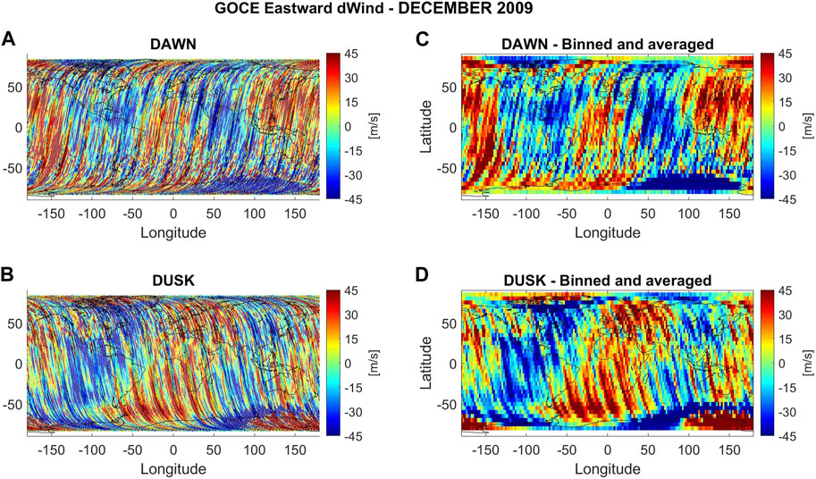
FIGURE 2. GOCE Eastward dWind for December 2009 for dawn (A,C) and dusk (B,D). dWind values calculated for each individual wind measurement are shown on the left, and the right shows the results after binning and averaging. Positive (negative) values correspond to eastward (westward) perturbations.

In order to analyze the longitudinal structures and to elucidate their underlying wave characteristics, a 1-D Fast Fourier Transform (FFT) was applied to the binned and averaged deviations separately in each latitude band. Here, the 1-D FFT will provide the different longitudinal frequencies present in the zonal wind perturbations. Because the 1-D FFT is applied separately in each 5° latitude band, the results for each band will be independent from each other.

For a fixed local solar time, the tidal perturbations $\stackrel{\sim }{T}$ can be expressed as (Oberheide et al., 2003):

where $T_{s,n}$ is the amplitude, ${\omega }_n$ is the wave frequency, $t$ is the local solar time, $t_{s,n}$ is the time of maximum amplitude with respect to 0° longitude, $\lambda$ is the longitude, $s$ is the zonal wavenumber and $n$ is the number of cycles per day ($n=1$ for the diurnal components, $n=2$ for the semidiurnal). This equation implies that when observing at a constant local time, the observed zonal wavenumber corresponds to $s^{\prime }=\left|s+n\right|$. Depending on the sign of $s$, the wave propagation is eastward for positive values of $s$ and westward for negative values of $s$.

Since the GOCE data are analyzed separately for dawn and dusk and thus correspond approximately to a fixed local time of ∼06 h for dawn and ∼18 h for dusk, the longitudinal variations in the GOCE data will appear as waves where the contributions from individual tides cannot be separated. Therefore, for example, both SE2 and DE3 will appear as part of a zonal wave-4 structure in the data, and their contributions will be combined in the FFT results. Since for migrating tides $=-n$ , and consequently $s^{\prime }=0$, their contribution appears as a constant in the tidal perturbations and becomes part of the median that we had subtracted from the zonal winds in our analysis. Consequently, the contribution of migrating tides is largely eliminated, and our results pertain to only non-migrating tides.

Figure 3 shows an example of the amplitude spectrum obtained from the FFT for the December 2011 period. Shown are the wave-m components up to wave-9. As already noted, these wave-m components do not pertain to a certain tidal wave, but instead are a combination of multiple tides. It is evident from Figure 3 that in this case the largest amplitudes are found in the first three wave components.

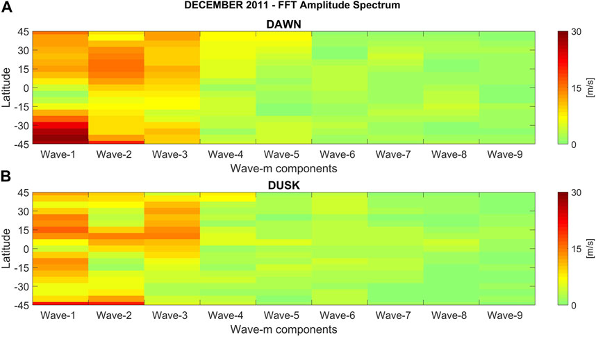
FIGURE 3. FFT amplitude spectrum for zonal wave-1 through wave-9 for GOCE zonal dWind for December 2011 during dawn (A) and dusk (B).

Figure 4 shows the wave amplitudes for December dawn conditions separately for each year from 2009 to 2012 (Figures 4A–D). Shown are the amplitudes for wave-1 to wave-9 as a global average (blue bars), averaged over the northern hemisphere (red bars), and averaged over the southern hemisphere (yellow bars). Here, the global values were obtained by averaging the individual wave-amplitudes in each latitude bin from −45° to 45° geographic latitude, and the northern/southern hemisphere averages were obtained by averaging the corresponding values from 0° to 45° and from 0° to −45°, respectively. It is interesting to note that during December 2009 the wave-1 amplitude in the northern hemisphere is more than twice the value found in the southern hemisphere. A similar hemispheric asymmetry can also be seen for wave-2 and wave-3 during December 2012. Figure 5 shows the same as Figure 4, but for dusk conditions. During this time, hemispheric asymmetries are present for wave-3 for December 2011 and for wave-2 and wave-3 during December 2012. Otherwise, the northern and southern averaged amplitudes are comparable to each other.

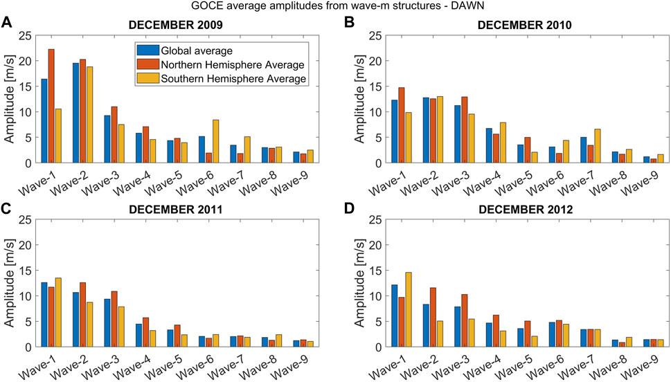
FIGURE 4. Average wave-m amplitudes for GOCE zonal dWind during dawn for wave-1 to wave-9 for December solstice 2009-2012 (A–D). The blue bars correspond to a global average (from -45° to 45° geographic latitude), the red bars represent the average for the northern hemisphere (0° to 45°) and the yellow bars correspond to the average in the southern hemisphere (0° to -45°).

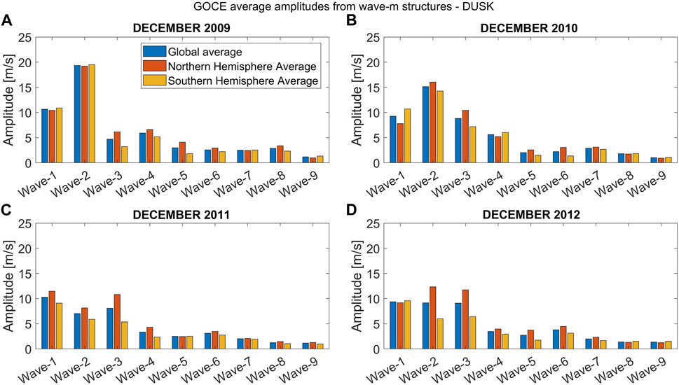
FIGURE 5. Same as Figure 4 but for dusk.

Figures 4, 5 also show that most of the wave amplitudes are concentrated in the first few wave numbers. In fact, our analysis shows that 75%–85% of the variability is represented by the first five components. As a consequence, we have limited our further analysis to only consider these first five wave-numbers.

Specifically, we have initially investigated the combined effect of wave-1 to wave-5 applying an inverse FFT (IFFT) after filtering out all contributions with zonal wavenumbers higher than 5. This was followed by a study of the individual effect of each wave-m component up to wave-5. For this all components of the FFT except the one corresponding to that particular wavenumber were filtered before the IFFT was performed. This step was repeated for all wave components from wave-1 through wave-5. In the following the combined contributions from wave-1 to wave-5 will be presented followed by a presentation of the individual contributions from wave-1 to wave-5.

4 Total zonal wind perturbations from wave-1 to wave-5

The total December GOCE zonal wind perturbations (dWind) obtained from the IFFT produced by the contributions from wave-1 through wave-5 are separately shown for each year from 2009 to 2012 as a function of latitude and longitude in the first four rows of Figure 6. Figures 6A–D correspond to dawn and Figures 6E–H to dusk conditions. Positive (negative) values are shown as red (blue) colors and correspond to eastward (westward) perturbations. Figures 6I, J show the corresponding model results obtained from CTMT that will be discussed in Section 6.

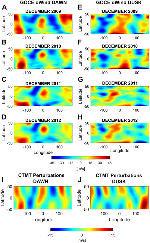
FIGURE 6. GOCE zonal dWind for December solstice for years 2009 to 2012 (A–H), and CTMT zonal wind perturbations (I,J) for December solstice 2011, during dawn (left column) and dusk (right column). Values correspond to the combined contributions from zonal wave-1 through wave-5. Positive (negative) values correspond to eastward (westward) perturbations.

In general, the total GOCE zonal wind perturbations at dawn remarkably resemble each other from one year to the next. During dusk, the GOCE zonal wind perturbations also show a good agreement for the low solar flux years 2009 and 2010 and as well as for the higher solar flux years 2011 and 2012. However, a clear change in the global pattern can be seen from 2010 to 2011. In the following sections, the global perturbation patterns are presented and agreements and differences from year to year are described in more detail.

4.1 Total zonal wind perturbations during dawn

The total December 2009 GOCE zonal wind perturbations at low- and mid-latitudes during dawn are shown in Figure 6A. The perturbations range from about −40 m/s to 50 m/s and exhibit a clear longitudinal structure consisting of four distinct bands. These bands alternate between eastward and westward perturbations and are generally tilted westward with increasing latitude (north-west alignment).

The first band exhibits eastward perturbations and is centered at about −160° longitude. The band shows two local maxima near 35° and −35° latitude that reach peak values of ∼45 m/s and ∼40 m/s, respectively.

The second band (westward perturbations) extends in the northern hemisphere from about −130° to about −30° longitude and forks into two branches resembling a Y-shaped structure centered at about −80° longitude. The peak values in this structure range from −10 m/s to −30 m/s. In the southern hemisphere, the band becomes narrower, extending from ∼-100° to ∼-50° with wind perturbations ranging from about −10 m/s to −30 m/s between about −10° and −50° latitude. Near the equator, from about 0° to −10° latitude, the wind perturbations in this band are small, with values of about −10 m/s.

The third band (eastward perturbations) is centered at about −10° longitude and depicts a more localized structure extending between ∼±30° latitude and −35° and 15° longitude. This structure exhibits wind perturbations ranging from about 10 m/s to 30 m/s.

The fourth band (westward perturbations) is centered at about 50° with wind perturbations between about −20 m/s to −40 m/s.

An additional eastward structure can be seen, centered at about 130° longitude. This structure, which is most apparent in the northern hemisphere, appears to be connected to the first band described above. The structure is located between 100° and 160° longitude and shows wind perturbations ranging from about 10 m/s to 40 m/s. In the southern hemisphere, the wind perturbations associated with this structure decrease to values of about 5 m/s.

The dawn GOCE wind perturbations for December 2010 for low- and mid-latitudes are shown in Figure 6B and also range from about −40 m/s to 50 m/s. A similar range of values is also found during December 2011 (Figure 6C), while during December 2012 (Figure 6D) the eastward peak values slightly reduce to about 40 m/s. The longitudinal structure observed in December 2009 can be identified in the subsequent years, but with noticeable changes.

The first eastward band, centered at around −160° longitude, is still present in 2010, but contrary to the 2009 results, the peak wind perturbations in the southern hemisphere are larger (∼50 m/s) compared to the northern hemisphere (∼27 m/s). These two maxima are also present in 2011 and 2012 but are no longer part of a distinct continuous band, but instead break into two isolated peaks. These isolated structures do not exhibit significant changes from 2011 to 2012. The peak values in 2011 are 30 m/s for the northern hemisphere peak and 45 m/s for the southern hemisphere maximum. For 2012 these peaks slightly reduce with values of 25 m/s and 40 m/s, respectively.

The second longitudinal band, which consists of westward perturbations, is present in 2010 as well, but significant differences are observed. The values in the northern hemisphere reach ∼ −40 m/s and the band is tilted eastward with increasing latitude (north-east alignment). This portion of the structure persists through 2011 and 2012, maintaining a remarkably similar shape and magnitude. In the southern hemisphere the zonal wind perturbations for 2010 are around −15 m/s, whereas in 2011 their magnitudes become much higher, reaching values of about −40 m/s. In 2012 they decrease again to about −15 m/s.

The third band (eastward perturbations) becomes more localized in 2010 and is only present in the northern hemisphere between 0° and 40° latitude, with magnitudes near 30 m/s. During 2011 and 2012 this structure remains nearly unchanged.

The fourth band (westward perturbations) is still present in 2010, but with smaller magnitudes overall. In the northern hemisphere it reaches values of −20 m/s and in the southern hemisphere the values are reduced to about −10 m/s to −15 m/s. In 2011 and 2012 this band nearly disappears at low latitudes (peak values of about −5 m/s) but is present at mid-latitudes in the southern hemisphere with values of the order of −20 m/s, connecting with the second longitudinal band at these latitudes.

The additional eastward structure that appeared connected to the first eastward band for 2009 gradually fades in the subsequent years, reducing from about 30 m/s in 2010 to about 15 m/s in 2011 and 2012.

4.2 Total zonal wind perturbations during dusk

The low and mid-latitude GOCE zonal wind perturbations for December 2009 during dusk are shown in Figure 6E and range from −40 m/s to 45 m/s. Similar to dawn, a clear longitudinal banded structure can also be identified during dusk with four bands alternating between eastward and westward perturbations. This time, however, the bands are generally tilted eastward with increasing latitude (north-east alignment).

The first band presents westward perturbations, and it is centered at about −90° longitude. The wind perturbations range from −20 m/s to −40 m/s. Although the width of the band changes with latitude, it spans on average approximately 65° of longitude.

The second band (eastward perturbations) is centered around 10° longitude, with the zonal wind perturbations ranging from 20 m/s to 40 m/s.

The third band presents westward perturbations and is composed of one localized maximum in each hemisphere. The northern hemisphere peak is located between 30° and 50° latitude and 90° to 135° longitude with peak values of about −20 m/s to −30 m/s. The southern hemisphere maximum is located between −5° and −50° latitude and 60° to 100° longitude. Here, the perturbations are of the order of −20 m/s. It is interesting to note that even though the general orientation of the bands is north-east, this particular structure exhibits a north-west orientation.

The fourth band presents eastward perturbations consisting of three maxima. The first peak is centered at about 180° longitude and 35° latitude and has a width of 20° in latitude and 50° in longitude. It has the highest values of perturbations within the band, ranging from 30 m/s to 40 m/s. The second maximum presents perturbations of about 15 m/s and is located between 135° and 175° longitude and −15° to −5° latitude. The third maximum has magnitudes of the order of 20 m/s and is present from 125° to 160° longitude and −30° to −40° latitude.

The dusk GOCE zonal wind perturbations for December 2010 (Figure 6F) are very similar to the corresponding 2009 results and also range from −40 m/s to 45 m/s. Some differences between the two years can be seen in the first band (westward perturbations) with smaller perturbation values (less than 5 m/s) during 2010 in the latitude range from 30° to 35° latitude and generally smaller westward perturbations in the southern hemisphere. Furthermore, although the second band (eastward perturbations) is still present in the southern hemisphere in December 2010 with wind perturbations of about 20 m/s to 45 m/s, a break-up into separate structures is seen in the northern hemisphere with overall lower perturbation values of about 20 m/s. The third band (westward perturbations) is also observed in the 2010 wind perturbations, with many of the same characteristics present in 2009. The band consists of two peaks, one in each hemisphere. The northern hemisphere maximum is located between 20° and 60° latitude and wind perturbations of about −20 m/s to −35 m/s. In the southern hemisphere the peak extends from about −40° to −5° latitude with wind perturbations ranging from −15 m/s to −20 m/s. Finally, the fourth band (eastward perturbations) is more continuous in 2010 where it extends from −20° to 50° latitude with wind perturbations ranging from 20 m/s to 35 m/s.

The dusk GOCE zonal wind perturbations for December 2011 and 2012 (Figures 6G, H) also range from −40 m/s to 45 m/s. The longitudinal structures observed during these later years, however, considerably differ from those observed during the earlier years and the banded structure is not as clearly defined in 2011 and 2012.

In particular, the first westward band that was observed during the earlier years, is not present in the southern hemisphere and consists in the northern hemisphere of localized peaks with wind perturbations that range from −20 m/s to −40 m/s in 2011 and from −20 m/s to −35 m/s in 2012. The second band (eastward perturbations) has shifted westward when compared to the earlier years and is now centered at about −50° longitude with magnitudes that range from 20 m/s to 40 m/s in 2011 to values of 20 m/s to 25 m/s in 2012. This band also exhibits a strong north-east alignment in contrast to the earlier years. The third band (westward perturbations) has become more localized in latitude during 2011 and 2012 with peaks approximately located between 20° and 40° and −5° and −25° latitude, respectively. Here, the peak wind perturbations are about −20 m/s to −30 m/s in the northern hemisphere and −15 m/s to −20 m/s in the southern hemisphere. Finally, the fourth band (eastward perturbations) is only present in 2011 for latitudes northward of about 20° latitude with wind perturbations of about 15 m/s to 20 m/s. During 2012 the band stretches from −5° to 50° of latitude, with wind perturbations of about 15 m/s to 25 m/s.

5 Individual contributions from wave-1 to wave-5

In the following sections the individual contributions of wave-1 to wave-5 to the total zonal wind perturbations are analyzed separately. The results are first shown for dawn followed by the corresponding results for dusk.

5.1 Individual contributions during dawn

The rows A through D of Figure 7 show the result of the separation of the dawn December 2009-2012 (top to bottom) GOCE zonal wind perturbations into their individual wave-m components with m ranging from 1 to 5 (left to right). Each wave-m structure is shown as a function of latitude and longitude. In general, the individual wave-m structures are remarkably similar from year to year in both phase and magnitude, but also exhibit differences in particular when comparing the individual wind perturbations for the low solar flux years (2009-2010) to those of the higher solar flux years (2011-2012).

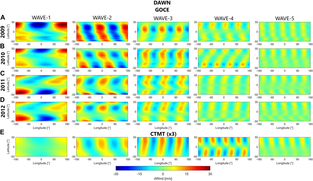
FIGURE 7. Individual zonal wave-1 to wave-5 zonal wind perturbations (left to right) during dawn. Rows (A–D) correspond to GOCE zonal dWind for December 2009 to 2012. Row (E) corresponds to CTMT zonal wind perturbations with the magnitudes multiplied by a factor of 3. Positive (negative) values correspond to eastward (westward) perturbations.

The zonal wind perturbation associated with wave-1 during dawn is shown in the first column and shows clear maxima (25–30 m/s) in the northern mid-latitudes (20°–50°) in 2009 and 2010. During 2011 and 2012 these structures gradually decrease to about 10–15 m/s and develop a banded structure with north-east alignment. In the southern hemisphere, from 2009 to 2012 the reverse process is observed.

Wave-2 (second column) presents a clear change from year-to-year. 2009 shows a banded structure with north-west alignment with magnitudes ranging from 15 to 25 m/s. In 2010, this structure evolves into more localized peaks in the northern (from 0° to 35° latitude) and southern hemisphere (−15° to −50° latitude) with slightly lower wind perturbation values when compared to 2009 (about 10 m/s to 20 m/s). In 2011 and 2012 the northern hemisphere peaks remain, but the alignment changes into a north-east direction for 2011 and more localized peaks in 2012. The southern hemisphere zonal wind perturbations diminish in magnitude progressively from 2009 to 2012, maintaining the north-west alignment, but nearly disappearing from −5° to −35° latitude in 2012.

The wave-3 component for 2009 (third column) exhibits localized peaks in the northern hemisphere, which evolve into a more banded structure with north-east alignment from 2010 to 2012. The phase of these structures is maintained for all years. The peak wind perturbations, however, change from 12 to 15 m/s in 2009, to 10–12 m/s in 2010 and 7–10 m/s in 2011 and 2012.

The 2009 wave-4 component presents bands (∼10 m/s) in the northern hemisphere (20°–40°). In the southern hemisphere the bands are located between −15° and 50° and the magnitudes are smaller (5–7 m/s). From 2010 to 2012 the bands are continuous for all latitudes with values ranging from 3 m/s to 7 m/s. In 2010 localized peaks can also be seen with magnitudes up to 10 m/s in the northern hemisphere (between 35° and 45°) and up to 12 m/s in the southern hemisphere (between −20° and −40°).

The zonal wind perturbations associated with wave-5 present a mostly north-aligned banded structure for all years (magnitudes ∼3–5 m/s), with more intense peaks (∼6 m/s) in the northern hemisphere for years 2010–2012. The amplitudes of these bands for 2009 are the same for both the northern and the southern hemisphere (∼3–5 m/s).

5.2 Individual contributions during dusk

The rows A through D of Figure 8 show the result of the separation of the dusk December 2009-2012 (top to bottom) GOCE zonal wind perturbations into their individual wave-m components with m ranging from 1 to 5 (left to right). Similar to the general morphology during dawn, the individual wave-m structures are again similar from year to year in both phase and magnitude, but this time the differences between the individual wind perturbations for the low solar flux years (2009-2010) and those for the higher solar flux years (2011-2012) become even more evident.

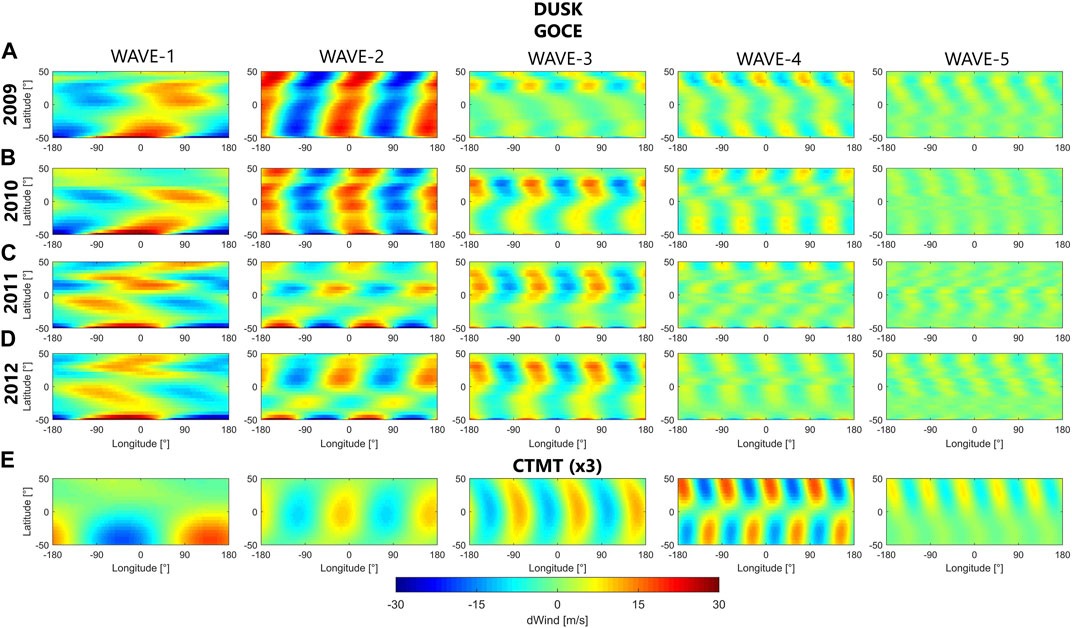
FIGURE 8. Same as Figure 7 but for dusk.

The zonal wind perturbations associated with wave-1 for 2009 during dusk are generally north-east aligned and show a banded structure with peaks (10–14 m/s) in the northern low and mid-latitudes and higher peaks (15–20 m/s) in the southern mid-latitudes. In 2010, the wave-1 zonal wind perturbations are very similar to the 2009 results, with some exceptions in the northern hemisphere where the peaks become more localized at low latitudes but maintaining similar magnitudes. The wave-1 responses in 2011 and 2012 are also very similar to each other but show significant differences to the prior years. In the southern mid-latitude, the maxima (10–12 m/s) are still present but exhibit a phase shift with respect to 2009 and 2010. Separate peaks are also observed in the higher southern (∼20 m/s) and northern latitudes (10–14 m/s).

The wave-2 response for 2009 shows a band structure with slight north-east alignment (∼20–25 m/s), which is also seen in 2010 but with smaller magnitudes (∼15–20 m/s). In 2011 and 2012 a banded structure is still present, but again significant differences to the prior years can be seen. In particular, more localized peaks with smaller amplitudes (∼10–12 m/s) and a stronger north-east alignment are observed. In 2011, the peaks are localized in the low (0°–20°) latitudes for the northern hemisphere and in the mid to higher (35°–50°) northern and southern latitudes. In 2012 larger amplitudes (12–15 m/s) are observed around 0°–40° in the northern hemisphere and −40° to −50° in the southern hemisphere.

The wave-3 zonal wind perturbations are very similar during the years from 2010 to 2012 but differ from the 2009 response. For 2009 localized peaks are present (∼10 m/s) in the northern hemisphere mid latitudes that become more extended toward the lower latitudes and stronger in magnitude during the subsequent years (10–16 m/s).

The wave-4 response for 2009, 2010, and 2012 exhibits a banded structure with north-west alignment. In 2011, the wave-4 response is more reminiscent of checkerboard pattern. The magnitudes of the wave-4 wind perturbations progressively decrease from 2009 to 2012 (from 5 to 10 m/s to 3–5 m/s).

The wave-5 responses for 2009, 2010, and 2012 are very similar to each other and show a banded structure with north-west alignment. In 2011, a checkerboard pattern can be seen in the northern hemisphere. The magnitudes are similar for all years (2–4 m/s).

6 Comparison with CTMT

In this section we will compare the GOCE results with simulations obtained from the Climatological Tidal Model of the Thermosphere (CTMT) (Oberheide et al., 2011) model. CTMT is an observation-based model that includes amplitudes and phases for six diurnal (DW2, DW1, D0, DE1, DE2, DE3) and eight semidiurnal (SW4, SW3, SW2, SW1, S0, SE1, SE2, SE3) tidal components for temperature, density, zonal, meridional and vertical winds from 80 to 400 km of altitude, pole-to-pole, and for moderate (F10.7 = 110 sfu) solar flux conditions. The model is based on Hough Mode Extensions to mean tidal diagnostics obtained from the TIMED Doppler Interferometer (TIDI) and the Sounding the Atmosphere using Broadband Emission Radiometry (SABER) instruments onboard the Thermosphere, Ionosphere, Mesosphere Energetics and Dynamics (TIMED) satellite. CTMT perturbations have been compared to satellite observations (Forbes et al., 2012; Lieberman et al., 2013b; Forbes et al., 2014; Forbes et al., 2022), used as boundary conditions for numerical experiments (e.g., Jones Jr et al., 2019) and to interpret and explain ground-based observations (e.g., Yuan et al., 2014).

The monthly CTMT amplitudes and phases are provided on a latitude/altitude grid with 5° latitude and 2.5 km altitude resolution. For our comparison of the GOCE zonal wind perturbations with those predicted by CTMT we have calculated for each individual GOCE data point the corresponding CTMT value. Specifically, we have interpolated the provided amplitude and phase data to the same days and locations of each individual GOCE observation using a linear interpolation in each dimension. Once the corresponding CTMT amplitudes and phases were obtained, the corresponding CTMT zonal wind perturbation for each individual tide was calculated using:

where ${\stackrel{\sim }{T}}_{n,s}$ is the tidal perturbation, n is the subharmonic of a solar day (n = 1 for diurnal tides and n = 2 for semidiurnal tides), s is the zonal wavenumber, $A_{n,s}$ is the amplitude, Ω is the rotation rate of the Earth, $t_L$ is the local solar time, λ is the longitude and ${\varphi }_{n,s}$ is the phase. Finally, the individual tidal components were added to obtain the total simulated zonal wind perturbation.

When investigating the longitudinal variations in the CTMT simulated zonal wind perturbations at a fixed local time the contributions from migrating tides appear as a constant and longitudinal variations are only due to non-migrating tidal components that will appear as a wave-m structures spanning from wave-1 to wave-5. In particular, D0, DW2, SW1 and SW3 will appear as a wave-1. Wave-2 will be comprised of DE1, S0 and SW4. Wave-3 will be composed of DE2 and SE1. DE3 and SE2 will appear as a wave-4. SE3 is the only component in CTMT that will appear as a wave-5.

Once the CTMT perturbations were calculated, the same steps performed on the GOCE zonal wind perturbations described in Section 3 were applied to the simulated CTMT zonal wind perturbations.

6.1 Comparison of combined contributions from wave-1 to wave-5

The top four rows of Figure 6 show the GOCE zonal wind perturbations for December 2009 to 2012 as already described in Section 4. Figures 6I, J show the corresponding CTMT zonal wind perturbations for dawn and dusk, respectively. The CTMT model results correspond to the December 2011 time period, which is used as a proxy for all four years. CTMT is a climatological model and does not vary with solar flux or geomagnetic activity. Consequently, differences between the CTMT results for the other years are only due to the small difference in the individual 27-day time period (differences of a few days) and the small shift in local time of the GOCE orbit from year to year (about 20 min/year). As a result, the CTMT results for the different years only display a longitudinal shift that does not exceed 4° and differ by at most 20%.

A visual inspection of the left column of Figure 6 shows the very good agreement in the general morphology of the structures at dawn between the CTMT and the 2009 and 2010 GOCE zonal wind perturbations, especially in the northern hemisphere, where the observed longitudinal bands align within 10° of those seen in the model results. In particular, the two peaks that were observed in the first band of eastward perturbations in GOCE during December 2009 and 2010 are also present in the CTMT model results. Furthermore, the Y-shape structure seen in the second band of westward perturbations in GOCE are closely resembled in the CTMT results. And finally, the inverted Y-shaped structure seen in the CTMT results as the fourth band (westward perturbations) is similar to the one observed in the 2010 GOCE perturbations. This band presents a peak in the northern hemisphere and smaller values in the southern hemisphere.

However, even though there are striking similarities between the general morphology of the GOCE and CTMT zonal wind perturbations, there are also noticeable differences. Foremost, the magnitudes of the CTMT wind perturbations are only about one-third of the corresponding GOCE values (note the difference in the color scale for GOCE and CTMT in Figure 6). Also, one additional band with westward zonal wind perturbations that is not present in the GOCE observations can be seen in the CTMT results centered near 170° longitude. Additional noticeable differences are a peak in the second band in the CTMT results in the southern hemisphere that is not as clearly seen in the GOCE zonal perturbations, and the existence of a more continuous third band (eastward perturbations) spanning latitudes from 50° to −25, where the GOCE wind perturbations were more localized.

During dusk, the CTMT zonal wind perturbations (Figure 6J) show significant differences with the observed GOCE zonal wind perturbations. The structures present in the CTMT perturbations do not resemble the general morphology of the GOCE results for any of the years. This will be further discussed in Section 6.2 and Section 7.

6.2 Comparison of individual contributions from wave-1 to wave-5

In order to further compare and contrast the GOCE and CTMT zonal wind perturbations, we have calculated for each individual wave-1 through wave-5 the corresponding CTMT result as described in Section 3.

Row E in Figures 7, 8 shows the result of the separation into wave-m components of the CTMT zonal wind perturbations and the GOCE zonal wind perturbations up to wave-5 during dawn and dusk respectively, for December 2009 to 2012. In order for GOCE and CTMT results to display similar magnitudes, the CTMT results have been multiplied by a factor of three.

Figure 7 shows that the dawn CTMT wave-1 component (bottom left panel) exhibits a very similar general structure when compared to the corresponding GOCE wave-1 variations. This includes a very similar phase and alignment of the longitudinal structures. However, the magnitudes of the CTMT wave-1 perturbations are significantly smaller when compared to the corresponding GOCE values. This comparison also holds when evaluating the relative importance of the wave-1 structures to the total zonal wind perturbations. For CTMT, the wave-1 perturbations only constitute about ∼14%–20% of the total zonal wind perturbations whereas the GOCE wave-1 perturbations constitute about 50%–60%. This difference will be further discussed in Section 7.

The wave-2 component shows a good agreement between the CTMT and the GOCE zonal wind perturbations for all years, especially in the northern hemisphere. The CTMT zonal wind perturbations present a structure of localized peaks (∼4 m/s) in the northern hemisphere between 0° and 50° of latitude with smaller perturbations (∼2 m/s) in the southern hemisphere forming a band that has a north-west orientation. The CTMT zonal wind perturbations are mostly aligned in longitude during all GOCE years (within ±10°).

The CTMT wave-3 component during dawn shows good agreement with the GOCE results in the northern hemisphere for 2010, 2011, and 2012, presenting a banded structure with north-east alignment. The model results present magnitudes of 3–5 m/s and the phase is also within ±5° of the GOCE 2010 results and within ±10°of the 2011 and 2012 results.

The CTMT wave-4 components show a checkered pattern of eastward and westward perturbations with magnitudes of about 4–5 m/s, with a separation (from −5° to 5°) near the geographic equator where the magnitudes get close to zero. This general structure agrees well with the 2009 wave-4 GOCE zonal wind perturbations.

For wave-5, the CTMT wind perturbations only consist of one tidal component, namely, SE3. For this component, CTMT agrees well with the corresponding GOCE zonal wind perturbations in the northern hemisphere where it presents a banded structure with values of ∼2.5 m/s. In the southern hemisphere, the wave-5 CTMT perturbations become very small with values less than 0.5 m/s. A similar hemispheric variation can also be seen in the wave-5 GOCE zonal wind perturbations during the years 2010–2012, with higher values in the northern hemisphere (∼5–6 m/s) than in the southern hemisphere (magnitudes up to ∼3 m/s).

As noted above, the total CTMT perturbations at dusk, as shown in Figure 6, did not resemble the corresponding GOCE perturbations. Figure 8 reveals that, in particular, the wave-1 component for dusk displays large differences from the corresponding GOCE wave-1 structure. In the southern hemisphere, CTMT presents large eastward and westward perturbations that maximize near −45° and 135° longitude, respectively, which appear nearly entirely out of phase with the corresponding GOCE pattern. In the northern hemisphere, the CTMT wave-1 structure practically vanishes, whereas GOCE shows significant perturbation values.

For wave-2, the CTMT results show a banded structure, albeit with smaller relative amplitudes, that agrees reasonably well with the GOCE pattern especially during the years 2009 and 2010. However, the CTMT values maximize at lower latitudes (between −20° and 20° latitude) whereas the GOCE perturbations during these years are uniformly extended over the entire latitude range. For the years 2011 and 2012 the phase of the CTMT and GOCE wave-2 pattern agrees well in the northern hemisphere, but the structures are out of phase in the southern hemisphere.

The dusk wave-3 component for CTMT presents structures with semicircular shapes centered at the equator that do not agree well with the GOCE results. Similarly, the CTMT wave-4 presents a checkered pattern, with a separation (from −5° to 5°) at the geographic equator, which also does not agree well with GOCE. However, the CTMT wave-5 pattern agrees well with GOCE during the years 2009, 2010 and 2012.

7 Summary and discussion

We have used low-to mid-latitude zonal wind observations from 2009 to 2012 obtained by the GOCE satellite near 260 km altitude during geomagnetically quiet times to investigate the interannual variation of the longitudinal variability of the zonal wind near dawn and dusk. The focus of the study was to investigate the year-to-year progression of the longitudinal variability in the GOCE zonal winds during December solstice produced by nonmigrating atmospheric tides. For each year the contributions from zonal wave-1 to wave-5 structures were separately determined and compared. The GOCE longitudinal zonal wind variations were also compared with corresponding results obtained from the CTMT model.

To determine the longitudinal variation in the GOCE zonal wind measurements, a 27-day window (one solar rotation) was selected for each year and the data were separately analyzed for dawn and dusk from −50° to 50° geographic latitude. The temporal and spatial variability of the zonal winds was then presented as a variation about the zonal mean values and decomposed into its underlying wave-m structures using a Fourier analysis. This approach largely eliminated the contribution of migrating tides from our analysis but also precluded us from separating the longitudinal variations into their individual tidal components. Consequently, our zonal wind perturbations appear as zonal wave-m structures that result from the superposition of individual non-migrating tidal components. It is important to highlight that in this methodology, the Fourier analysis is applied to each latitude band individually; therefore, the results for each one of these bands are independent of each other. The coherence between the adjacent latitude bands presented in Figures 6–8 gives confidence in the structures observed.

It was found that 75%–85% of the longitudinal zonal wind variability could be explained as due to waves that generate zonal wave-m structures with m up to 5, and therefore, this was the cutoff used in our Fourier analysis. A clear interannual progression of the individual wave components could be observed in the resulting structures.

In general, the total GOCE zonal wind perturbations at dawn remarkably resemble each other from one year to the next. During dusk, the GOCE zonal wind perturbations also show a good agreement for the low solar flux years 2009 and 2010 as well as for the higher solar flux years 2011 and 2012. However, a clear change in the global pattern can be seen from 2010 to 2011. Note that the F10.7 solar flux values during 2009 and 2010 were lower than during 2011 and 2012 and the change in the pattern might be related to the change in solar flux. A similar good agreement in the total GOCE zonal wind perturbations can also be observed for June 2010 and June 2011 (shown in Supplementary Figure S1). As pointed out above, the average F10.7 solar flux during these two June periods also only differs by 20 sfu.

Both ENSO and the QBO are also known to produce year-to-year variability on atmospheric tides (e.g., Oberheide et al., 2009; Warner and Oberheide, 2014). As mentioned above, the GOCE results for each December pair 2009-2010 and 2011-2012 are similar. Figure 1B shows, however, that the ONI values for 2009 and 2010 are very different and correspond to moderate El Niño and strong La Niña conditions, respectively. December 2011 presents moderate La Niña conditions, and December 2012 does not present either. From Figure 1C, it is also evident that the QBO U30 index is different for the December 2009 and 2010 pair. Differences are also observed in the index for the June 2010 and 2011 pair. Based on these observations, it appears that the year-to-year variations seen in GOCE are not the result of either variations in ENSO or the QBO. During dawn, the total December solstice GOCE zonal wind perturbations at low- and mid-latitudes range from about −40 m/s to 50 m/s and exhibit a clear longitudinal structure consisting of four distinct bands. These bands alternate between eastward and westward perturbations and are generally tilted westward with increasing latitude (north-west alignment). The individual wave-m structures during dawn are also remarkably similar from year to year in both phase and magnitude, but also exhibit differences when comparing the individual wind perturbations for the low solar flux years (2009-2010) to those of the higher solar flux years (2011-2012).

During dusk, the low and mid-latitude GOCE zonal wind perturbations for December solstice also range from −40 m/s to 45 m/s. Like dawn, a clear longitudinal banded structure can be identified at with four bands alternating between eastward and westward perturbations. This time, however, the bands are generally tilted eastward with increasing latitude (north-east alignment). Similar to the general morphology during dawn, the individual wave-m structures are again similar from year to year in both phase and magnitude, but this time the differences between the individual wind perturbations for the low solar flux years (2009-2010) and those for the higher solar flux years (2011-2012) become even more evident. Here again, a similar result is found for the two June periods where the individual wave-m structures resemble each other year-to-year (see Supplementary Figure S2 for dawn and Supplementary Figure S3 for dusk).

Some of the characteristics just described are observed in a companion paper by Molina and Scherliess (2023), who have used the same GOCE zonal wind observations to determine their spatial and temporal correlations. In particular, it is mentioned that the longitudinal/temporal correlations for December 2009 indicate that the structures that generate them have a north-west orientation during dawn (Figure 10 in their paper) and north-east orientation during dusk (their Figure 11). It is noteworthy that this is observed in Figure 6 of this paper as the general orientation of the longitudinal bands for December 2009 for dawn and dusk, respectively. The zonal wave structures up to wave-5 obtained in this work were also subtracted from the associated perturbations, and the longitude/time correlation coefficients were subsequently calculated for their study. The resulting correlation coefficients (Figures 12 to 15 in their paper) suggest that the zonal wave-m structures described in this paper are largely responsible for the original patterns observed in their longitudinal/temporal correlations.

A comparison of the GOCE results with simulations obtained from the CTMT model has revealed a very good agreement between the CTMT and the December 2009 and 2010 GOCE zonal wind perturbations at dawn, especially in the northern hemisphere, where the observed longitudinal bands align within 10° of those seen in the model results. However, even though there are striking similarities between the general morphology of the GOCE and CTMT zonal wind perturbations, there are also noticeable differences. During dusk the CTMT zonal wind perturbations show significant differences with the observed GOCE zonal wind perturbations. The structures present in the CTMT perturbations do not resemble the general morphology of the GOCE results for any of the years. In particular, the CTMT wave-1 component significantly differs from the GOCE results (this can also be seen in Supplementary Figures S2, S3 for June solstice). There could be several reasons for this discrepancy. Oberheide et al. (2011) compared the CTMT densities near 400 km altitude with those obtained from the CHAMP satellite and found that the agreement with the tidal components DW2, D0, SW1, and SW3 was poor. As mentioned before, these are also the components that constitute the wave-1 structure. They suggest that the observed differences are the result of the generation mechanisms of these tidal components, which are believed to be generated by hydromagnetic coupling between various waves (Jones et al., 2013) which is not captured by the CTMT formulation. Part of the discrepancy between GOCE and CTMT at dusk might also be the result of our use of a geographic coordinate system in our analysis. Liu et al. (2016) found the presence of wind jets aligned with the magnetic equator in GOCE zonal winds. Zhang et al. (2018) used CHAMP zonal winds together with TIEGCM model simulations to investigate the effect of the geomagnetic field on longitudinal variations observed in zonal winds. They conclude that the large-scale longitudinal variations are produced by the geomagnetic field structure and might be the result of temporal variations of ion drag and pressure gradient forces. Indeed, the variation captured by TIEGCM in their Figure 10 is reminiscent of a wave-1 structure for both dawn and dusk.

Regarding the differences in magnitudes of the CTMT wind perturbations, which are only about one-third of the corresponding GOCE values, it needs to be noted that it is not clear whether this difference is the result of an underestimation of zonal wind perturbations by CTMT or due to a systematic overestimation of the GOCE wind data or both. Jiang et al. (2021) for example, compared GOCE zonal winds with wind observations obtained from ground-based Fabry-Perot Interferometer (FPI) measurements at low and mid latitudes and reported an overall overestimation of the GOCE winds when compared to the ground-based data. They found that the magnitudes from GOCE are generally larger than the FPI winds by a factor of 1.37–1.69, consistent with FPI comparisons at high latitudes where factors of 1.2–2.0 were reported by Kärräng (2015), albeit using an earlier version of the GOCE data. An earlier version of the data was also used by Dhadly et al. (2017, Dhadly et al., 2019) who reported a magnetic latitude-depended bias in the GOCE data when compared to WINDII, SDI and FPI observations at high latitudes. The possible presence of a bias in the GOCE data, however, would have only affected our zonal mean values and consequently would have been eliminated when calculating the wind perturbations. A factor difference, however, would also affect our perturbation values and consequently our reported values should be scaled by this factor.

Finally, it should be noted that our analysis only pertains to December and June solstice conditions at dawn and dusk and an investigation of the year-to-year progression of the longitudinal variability of the zonal wind during other seasons and local times needs to be performed in the future.

Data availability statement

Publicly available datasets were analyzed in this study. This data can be found here: https://earth.esa.int/eogateway/catalog/goce-thermosphere-data, https://doi.org/10.5281/zenodo.5541913, https://omniweb.gsfc.nasa.gov/form/dx1.html, https://www.cpc.ncep.noaa.gov/data/indices/.

Author contributions

IM and LS contributed to the conception and design of the study. IM conducted the analysis. All authors contributed to the article and approved the submitted version.

Funding

This research was partially supported by NASA Headquarters under the NASA Earth and Space Science Fellowship Program (NESSF/FINESST), GRANT 80NSSC17K0431; National Science Foundation grant AGS-1651461 to Utah State University and NASA grant 80NSSC20K0191 to Utah State University.

Acknowledgments

The GOCE data used in this work are publicly available and provided by the European Space Agency (ESA) and can be found at https://earth.esa.int/eogateway/catalog/goce-thermosphere-data. We acknowledge use of NASA/GSFC’s Space Physics Data Facility’s OMNIWeb service to obtain the F10.7 cm radio flux and Kp index. We acknowledge the use of the ONI and QBO U30 index provided by the National Weather Service Climate Prediction Center. We gratefully acknowledge Dr J. Oberheide for making the Climatological Tidal Model of the Thermosphere freely available. The CTMT netCDF data files can be found at https://doi.org/10.5281/zenodo.5541913. Part of this work is included in IM’s PhD dissertation, which can be found at https://digitalcommons.usu.edu/etd/8671/.

Conflict of interest

The authors declare that the research was conducted in the absence of any commercial or financial relationships that could be construed as a potential conflict of interest.

Publisher’s note

All claims expressed in this article are solely those of the authors and do not necessarily represent those of their affiliated organizations, or those of the publisher, the editors and the reviewers. Any product that may be evaluated in this article, or claim that may be made by its manufacturer, is not guaranteed or endorsed by the publisher.

Supplementary material

The Supplementary Material for this article can be found online at: https://www.frontiersin.org/articles/10.3389/fspas.2023.1214612/full#supplementary-material

References

Bamston, A. G., Chelliah, M., and Goldenberg, S. B. (1997). Documentation of a highly ENSO-related SST region in the equatorial pacific: research note. Atmosphere-ocean 35 (3), 367–383. doi:10.1080/07055900.1997.9649597
Bruinsma, S., and Biancale, R. (2003). Total densities derived from accelerometer data. J. Spacecr. Rockets 40 (2), 230–236. doi:10.2514/2.3937
Dhadly, M., Emmert, J., Drob, D., Conde, M., Doornbos, E., Shepherd, G., et al. (2017). Seasonal dependence of northern high-latitude upper thermospheric winds: A quiet time climatological study based on ground-based and space-based measurements. J. Geophys. Res. Space Phys. 122 (2), 2619–2644. doi:10.1002/2016ja023688
Dhadly, M. S., Emmert, J. T., Drob, D. P., Conde, M. G., Aruliah, A., Doornbos, E., et al. (2019). HL-TWiM empirical model of high-latitude upper thermospheric winds. J. Geophys. Res. Space Phys. 124 (12), 10592–10618. doi:10.1029/2019ja027188
Dhadly, M. S., Emmert, J. T., Jones, M., Doornbos, E., Zawdie, K. A., Drob, D. P., et al. (2020). Oscillations in neutral winds observed by GOCE. Geophys. Res. Lett. 47 (17), e2020GL089339. doi:10.1029/2020gl089339
Doornbos, E., Van Den Ijssel, J., Luhr, H., Forster, M., and Koppenwallner, G. (2010). Neutral density and crosswind determination from arbitrarily oriented multiaxis accelerometers on satellites. J. Spacecr. Rockets 47 (4), 580–589. doi:10.2514/1.48114
Forbes, J. M. (2007). Dynamics of the thermosphere. J. Meteorological Soc. Jpn. Ser. II 85, 193–213. doi:10.2151/jmsj.85b.193
Forbes, J. M., Oberheide, J., Zhang, X., Cullens, C., Englert, C. R., Harding, B. J., et al. (2022). Vertical coupling by solar semidiurnal tides in the thermosphere from ICON/MIGHTI measurements. J. Geophys. Res. Space Phys. 127 (5), e2022JA030288. doi:10.1029/2022ja030288
Forbes, J. M. (1996). Planetary waves in the thermosphere-ionosphere system. J. geomagnetism Geoelectr. 48 (1), 91–98. doi:10.5636/jgg.48.91
Forbes, J. M., Zhang, X., and Bruinsma, S. L. (2014). New perspectives on thermosphere tides: 2. Penetration to the upper thermosphere. Earth, Planets Space 66 (1), 122–211. doi:10.1186/1880-5981-66-122
Forbes, J. M., Zhang, X., and Bruinsma, S. (2012). Middle and upper thermosphere density structures due to nonmigrating tides. J. Geophys. Res. Space Phys. 117 (A11). doi:10.1029/2012ja018087
Forbes, J. M., Zhang, X., Hagan, M. E., England, S. L., Liu, G., and Gasperini, F. (2017). On the specification of upward-propagating tides for ICON science investigations. Space Sci. Rev. 212, 697–713. doi:10.1007/s11214-017-0401-5
Fritts, D. C., and Alexander, M. J. (2003). Gravity wave dynamics and effects in the middle atmosphere. Rev. Geophys. 41 (1). doi:10.1029/2001rg000106
Gasperini, F., Forbes, J. M., Doornbos, E. N., and Bruinsma, S. L. (2015). Wave coupling between the lower and middle thermosphere as viewed from TIMED and GOCE. J. Geophys. Res. Space Phys. 120 (7), 5788–5804. doi:10.1002/2015ja021300
Häusler, K., and Lühr, H. (2009). Nonmigrating tidal signals in the upper thermospheric zonal wind at equatorial latitudes as observed by CHAMP. Ann. Geophys. 27, 2643–2652. doi:10.5194/angeo-27-2643-2009
Immel, T. J., Sagawa, E., England, S. L., Henderson, S. B., Hagan, M. E., Mende, S. B., et al. (2006). Control of equatorial ionospheric morphology by atmospheric tides. Geophys. Res. Lett. 33 (15), L15108. doi:10.1029/2006gl026161
Jiang, , Guoying, , Xiong, C., Stolle, C., Xu, J., and Yuan, W. (2021). Comparison of thermospheric winds measured by GOCE and ground-based FPIs at low and middle latitudes. J. Geophys. Res. Space Phys. 126 (2), e2020JA028182.
Jones, M., Forbes, J. M., Hagan, M. E., and Maute, A. (2013). Non-migrating tides in the ionosphere-thermosphere: in situ versus tropospheric sources. J. Geophys. Res. Space Phys. 118 (5), 2438–2451. doi:10.1002/jgra.50257
Jones, M., Forbes, J. M., and Sassi, F. (2019). The effects of vertically propagating tides on the mean dynamical structure of the lower thermosphere. J. Geophys. Res. Space Phys. 124 (8), 7202–7219. doi:10.1029/2019ja026934
Kärräng, P. (2015). Comparison of thermospheric parameters from space-and ground-based instruments (MS thesis). Kiruna, Sweden: Luleå University of Technology.
Lieberman, R. S., Akmaev, R. A., Fuller‒Rowell, T. J., and Doornbos, E. (2013a). Thermospheric zonal mean winds and tides revealed by CHAMP. Geophys. Res. Lett. 40 (10), 2439–2443. doi:10.1002/grl.50481
Lieberman, R. S., Oberheide, J., and Talaat, E. R. (2013b). Nonmigrating diurnal tides observed in global thermospheric winds. J. Geophys. Res. Space Phys. 118 (11), 7384–7397. doi:10.1002/2013ja018975
Lindzen, R. S. (1981). Turbulence and stress owing to gravity wave and tidal breakdown. J. Geophys. Res. Oceans 86 (C10), 9707–9714. doi:10.1029/jc086ic10p09707
Liu, H., Doornbos, E., and Nakashima, J. (2016). Thermospheric wind observed by GOCE: wind jets and seasonal variations. J. Geophys. Res. Space Phys. 121 (7), 6901–6913. doi:10.1002/2016ja022938
Liu, H. L., Wang, W., Richmond, A. D., and Roble, R. G. (2010). Ionospheric variability due to planetary waves and tides for solar minimum conditions. J. Geophys. Res. Space Phys. 115 (A6). doi:10.1029/2009ja015188
March, G., Doornbos, E. N., and Visser, P. N. A. M. (2019a). High-fidelity geometry models for improving the consistency of CHAMP, GRACE, GOCE and Swarm thermospheric density data sets. Adv. Space Res. 63 (1), 213–238. doi:10.1016/j.asr.2018.07.009
March, G., Visser, T., Visser, P. N. A. M., and Doornbos, E. N. (2019b). CHAMP and GOCE thermospheric wind characterization with improved gas-surface interactions modelling. Adv. Space Res. 64 (6), 1225–1242. doi:10.1016/j.asr.2019.06.023
Miyahara, S., Yoshida, Y., and Miyoshi, Y. (1993). Dynamic coupling between the lower and upper atmosphere by tides and gravity waves. J. Atmos. Terr. Phys. 55 (7), 1039–1053. doi:10.1016/0021-9169(93)90096-h
Molina, I. (2022). Variability of thermospheric zonal winds near dawn and dusk (PhD dissertation). Logan, Utah: Utah State University.
Molina, I., and Scherliess, L. (2023). Spatial and temporal correlations of thermospheric zonal winds from GOCE satellite observations. Frontiers in Astronomy and Space Sciences 10, 1214591.
Oberheide, J., Forbes, J. M., Häusler, K., Wu, Q., and Bruinsma, S. L. (2009). Tropospheric tides from 80 to 400 km: propagation, interannual variability, and solar cycle effects. J. Geophys. Res. Atmos. 114 (D1). doi:10.1029/2009jd012388
Oberheide, J., Forbes, J. M., Zhang, X., and Bruinsma, S. (2011). Climatology of upward propagating diurnal and semidiurnal tides in the thermosphere. J. Geophys. Res. Space Phys. 116 (A11). doi:10.1029/2011ja016784
Oberheide, J., Hagan, M. E., Richmond, A. D., and Forbes, J. M. (2015). “Atmospheric tides,” in Encyclopedia of atmospheric Sciences. Second ed. China, (Academic Press), 287–297.
Oberheide, J., Hagan, M. E., and Roble, R. G. (2003). Tidal signatures and aliasing in temperature data from slowly precessing satellites. J. Geophys. Res. Space Phys. 108 (A2). doi:10.1029/2002ja009585
Sutton, E. K., Nerem, R. S., and Forbes, J. M. (2007). Density and winds in the thermosphere deduced from accelerometer data. J. Spacecr. Rockets 44 (6), 1210–1219. doi:10.2514/1.28641
Teitelbaum, H., and Vial, F. (1981). Momentum transfer to the thermosphere by atmospheric tides. J. Geophys. Res. Oceans 86 (C10), 9693–9697. doi:10.1029/jc086ic10p09693
Visser, T., March, G., Doornbos, E., De Visser, C., and Visser, P. (2019). Horizontal and vertical thermospheric cross-wind from GOCE linear and angular accelerations. Adv. Space Res. 63 (10), 3139–3153. doi:10.1016/j.asr.2019.01.030
Wang, W., Burns, A. G., and Liu, J. (2021). Upper thermospheric winds: forcing, variability, and effects. Up. Atmos. Dyn. energetics, 41–63. doi:10.1002/9781119815631.ch3
Warner, K., and Oberheide, J. (2014). Nonmigrating tidal heating and MLT tidal wind variability due to the El Niño–Southern Oscillation. J. Geophys. Res. Atmos. 119 (3), 1249–1265. doi:10.1002/2013jd020407
Yuan, T., Wang, J., Cai, X., Sojka, J., Rice, D., Oberheide, J., et al. (2014). Investigation of the seasonal and local time variations of the high-altitude sporadic Na layer (Nas) formation and the associated midlatitude descending E layer (Es) in lower E region. J. Geophys. Res. Space Phys. 119 (7), 5985–5999. doi:10.1002/2014ja019942
Keywords: neutral wind, thermosphere, ionosphere, tides, upper atmosphere dynamics, GOCE
Citation: Molina I and Scherliess L (2023) Longitudinal variability of thermospheric zonal winds near dawn and dusk. Front. Astron. Space Sci. 10:1214612. doi: 10.3389/fspas.2023.1214612
Received: 30 April 2023; Accepted: 07 September 2023;
Published: 29 September 2023.
Edited by:
Han-Li Liu, National Center for Atmospheric Research (UCAR), United StatesReviewed by:
Federico Gasperini, Orion Space Solutions LLC, United StatesHidekatsu Jin, National Institute of Information and Communications Technology, Japan
Copyright © 2023 Molina and Scherliess. This is an open-access article distributed under the terms of the Creative Commons Attribution License (CC BY). The use, distribution or reproduction in other forums is permitted, provided the original author(s) and the copyright owner(s) are credited and that the original publication in this journal is cited, in accordance with accepted academic practice. No use, distribution or reproduction is permitted which does not comply with these terms.
*Correspondence: Ludger Scherliess, ludger.scherliess@usu.edu