PyThea: An open-source software package to perform 3D reconstruction of coronal mass ejections and shock waves

1 Introduction

Coronal mass ejections (CMEs) are large expulsions of magnetized plasma from the Sun’s outer atmosphere, the corona, towards the interplanetary (IP) space, and they are the most spectacular eruptive phenomenon observed in the solar corona and one of the main drivers of space weather. Big CMEs can release a huge amount of plasma and magnetic flux into the IP space (e.g. Chen, 2011; Webb and Howard, 2012). CMEs can also drive shock waves (e.g. Ontiveros and Vourlidas, 2009; Frassati et al., 2019) and can cause very intense geomagnetic storms on Earth, which usually have a significant impact on ground-based and space-borne technological systems (Lakhina and Tsurutani, 2016; Temmer, 2021).

Our knowledge about CMEs and shock waves has significantly increased over the past several decades. The initiation processes, three-dimensional (3D) structure, evolution, and properties of CMEs and shock waves are very important and recurrent areas of heliospheric physics research (e.g. Balmaceda et al., 2020; Balmaceda et al., 2022; Rodríguez-García et al., 2022), since these are the main space weather drivers. In addition, a deeper understanding of the physical processes involved in these phenomena (e.g. Patsourakos and Vourlidas, 2012; Kwon and Vourlidas, 2017; Long et al., 2017) is essential to resolve fundamental scientific questions in heliophysics. This understanding also helps to elucidate the processes involved in other associated solar phenomena. For example, during the most energetic solar events, when fast CMEs and shock waves are observed, particles are accelerated at very high energies (e.g. Kouloumvakos et al., 2019; 2020a). Solar energetic particles (SEP) events are another important element of space weather and pose a significant hazard to the inner heliosphere, especially for those events with large intensity increases and high energy particles (e.g. Gómez-Herrero et al., 2015; Rodríguez-García et al., 2021).

CMEs and shock waves can be observed either by remote sensing instruments or can be measured in situ. Coronal transients are nowadays routinely observed in white light (WL) that is scattered by free electrons of the solar corona. These observations are provided by coronagraphs or heliospheric imagers onboard spacecraft located in near-Earth orbit. Observations of the solar corona from the Sun-Earth Connections Coronal and Heliospheric Investigation (SECCHI; Howard et al., 2008) onboard the Solar Terrestrial Relations Observatory (STEREO; Kaiser et al., 2008) have provided nearly simultaneous imaging of CMEs and other transients from different viewpoints for more than a decade. The three different perspectives provided by near-Earth spacecraft (e.g. the Solar Dynamics Observatory (SDO; Pesnell et al., 2012) and the Solar and Heliospheric Observatory (SOHO; Domingo et al., 1995)) and the two STEREO spacecraft allow us to reconstruct CMEs and shocks. However, since 2015, communications with STEREO-B were lost and currently STEREO consists of only one observatory–STEREO-A–that slowly catching up with Earth. Multiple viewpoint observations are essential to study the 3D structure and kinematics of the CMEs and shock waves, alleviating projection effects and reducing the uncertainty when determining the position and kinematics (Mierla et al., 2010).

Numerous previous studies have extensively used and relied on CME and shock wave 3D reconstructions to address top-level scientific questions. Most of the studies focus on examining the geometrical properties and kinematic parameters of CMEs and shock waves as they evolve in the solar corona. These studies contribute to addressing fundamental questions about CME initiation and energetics; the interaction of CMEs with coronal structures, the solar wind magneto-plasma, or other CMEs (CME-CME interaction) (Scolini et al., 2020; Palmerio et al., 2021); physics of collisionless shock waves in the corona (Kwon et al., 2014; Kwon and Vourlidas, 2017); initiation and development mechanisms of shocks (Mancuso et al., 2019); the relation of CMEs-shocks to solar flares; and many other CME or shock related subjects (e.g. Wood et al., 2011; Hess et al., 2020; Rouillard et al., 2020). Some studies have indirectly benefited from 3D reconstructions to address their overarching goals for another topic, other than the physics of CME and shock waves. These studies investigate, for example, the role of CMEs and shock waves to SEP acceleration and release to the heliosphere (e.g. Rouillard et al., 2016; Kouloumvakos et al., 2019, 2020b; Giacalone et al., 2020; Dresing et al., 2022), the wide distribution of SEPs in the heliosphere (e.g. Rouillard et al., 2012; Lario et al., 2014, 2016, 2017; Kouloumvakos et al., 2016; Zhu et al., 2018; Rodríguez-García et al., 2021; Kouloumvakos et al., 2022), and the connection of CMEs and shocks to solar radio emission (e.g. Type II, IV radio bursts; Zucca et al., 2018; Morosan et al., 2020; Kouloumvakos et al., 2021; Jebaraj et al., 2021) and solar gamma-ray bursts (Kouloumvakos et al., 2020a). CME and shock wave reconstruction can also play a critical role in space weather forecasting and nowcasting models. The propagation characteristics and kinematics of IP CMEs are key parameters to evaluate the impact of the events on Earth using space weather modelling.

The most widely used method to perform 3D reconstructions combines a geometrical model with the scraytrace code which is available in the Solarsoft library that uses the Interactive Data Language (IDL) to run it. IDL is a popular programming language in areas of science, however, a paid licence is needed to use it. Additionally, this 3D reconstruction process requires that the user download and process the data before the reconstruction. The users can use pairs or triplets of images from coronagraphs or extreme ultraviolet (EUV) imagers. Within the geometrical models, the graduated cylindrical shell (GCS; Thernisien et al., 2006; Thernisien, 2011) model is widely used to parameterize the 3D structure of a typical flux-rope shape like a CME. For shock waves, a spheroid or an ellipsoid model is extensively used to parameterize them (e.g. Kwon et al., 2014). The 3D reconstruction is then performed by overlaying, onto each imager, the grid of points parameterized from the geometrical model. The points are usually projected onto the plane-of-sky (POS) when using images from the coronagraphs. Then the user changes the model parameters until a good fit is achieved compared with the observations. The final 3D reconstruction has to reproduce the observed features at each observing point.

In this article, we present PyThea, a newly developed open-source software package that can be used to perform 3D reconstruction of coronal mass ejections and shock waves. The name of the package is inspired by the words Python and Thea. In Greek mythology, Thea, also called Euryphaessa “wide-shining”, is the Titaness of sight and the shining light of the clear blue sky and also the mother of Helios (the Sun), Selene (the Moon), and Eos (the Dawn). PyThea is developed and managed by A. Kouloumvakos. The source code of the package is provided in a publicly available GitHub repository¹. GitHub is a code hosting platform for version control and collaboration. This package is produced in Python and licensed under GPL-3.0 License². The main goal behind this package development is to provide to the community the functionality and tools needed to perform robust 3D reconstructions of CMEs and shock waves in Python programming language, which is one of the most widely used programming languages³. Python is a free-of-cost and open-source programming language, it is easy to learn and use, and it has a very active and supportive community.

The scope of this article is to introduce PyThea software package to the heliophysics community and present its main features. This presentation will be generic and independent of the package version. We start with a description of PyThea‘s python package structure and its core functionality. Then we show details on the application and the constructed Graphical User Interface (GUI). The user can use this application to perform a full analysis of an eruptive event by visualizing the remote sensing observations and performing the CME and shock wave reconstructions. In the last section, we discuss the current state of the package and future development.

2 PyThea software package

2.1 Overview

The PyThea software package is developed to provide the necessary tools to perform 3D reconstruction of CMEs and shock waves and determine their kinematics, using multi-spacecraft remote sensing observations. This package has been built in Python (≥3.8) with an extensive use of libraries available within the Python language ecosystem. PyThea has been tested in Unix based systems, however, PyThea is a platform-independent package. During the development and release process of the package, we follow a semantic versioning, which consists of three-part version numbers: major version, minor version, and patch. At the time of writing this article, PyThea‘s latest version is v0.6.6. This is primarily done to convey that there is a compatibility between releases. Every new version of PyThea is uploaded and registered in the Python Package Index (PyPI). This is a repository with a list of available software packages produced with the Python programming language.

The latest or specific versions of PyThea can be found and downloaded from PyPI⁴ or from the host GitHub repository. PyThea can be installed using pip, which is the package installer for Python and it is usually shipped along with it. The pip command installs PyThea package from PyPI by default. Like most python packages, to use PyThea it is required that some dependent packages have been installed. These dependent packages are installed automatically using pip. An installation using conda is also possible (see details in GitHub). conda is another package and environment management system, which helps to easily install packages and their dependencies. Unlike pip, conda checks the dependencies before the installation and identifies conflicts before they occur. We recommend for less experienced users to create a “virtual environment” in Python or conda⁵. before installing PyThea package. This is an easy process that allows the package to be installed in an isolated environment rather than globally.

We build PyThea using fundamental Python packages for data manipulation, scientific computing, and high level visualization that produce publication-quality figures. NumPy (Harris et al., 2020) and SciPy (Virtanen et al., 2020) are, for example, two foundational Python packages that are used to operate on data and deal with scientific computations. Both packages offer a comprehensive library of mathematical functions that can operate on arrays and matrices. Another example is Matplotlib (Hunter, 2007), which is a comprehensive plotting library for Python. To build the main application and the GUI, we used the Streamlit Python package. This is an open-source Python library that provides an easy way to create web applications. After the installation of the PyThea package, the web application can be launched using only one command in the terminal.

For the scientific data analysis, we use two core packages, Astropy (Astropy Collaboration et al., 2013; Astropy Collaboration et al., 2018) and SunPy (Mumford et al., 2020; The SunPy Community et al., 2020). These packages provide the functionality to read, process, and visualize astronomical data. Astropy includes many libraries that support scientific data analysis. In PyThea, we use two main functionality features from Astropy, the ability to use numbers with associated units (astropy.units) and to represent and transform between different coordinate systems (astropy.coordinates). From SunPy, we use the data search, retrieval, load, and visualization functionality. The most important subpackages are sunpy.net, which is used to retrieve the data, and sunpy.map, which provides the framework to load and visualize the data. Additionally, the sunpy.coordinates subpackage provides support to represent and transform between different coordinate systems used in solar physics.

In Figure 1, we present a typical workflow when analysing and reconstructing an event using PyThea. The first step is the data retrieval from multiple sources. Then, these data are processed and visualized so that the user can fit the geometrical model. The last step is the calculation of the kinematics and saving of the final fittings. In the following sections, we present information for each subprocess.

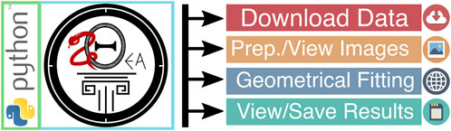
FIGURE 1. Semantic of PyThea‘s typical workflow for the analysis and reconstruction of an event.

2.2 Data acquisition and loading

PyThea provides functions to download and load solar data from selected imagers. The process relies on the data acquisition interface of SunPy, named Fido. It is a powerful interface that provides a unified way to perform data search and retrieval from multiple sources simultaneously. The primary data source for PyThea is the Virtual Solar Observatory (VSO; Hill et al., 2009). It is a tool developed to allow access to data from multiple solar data providers and different data sets from space-borne and ground-based instruments. The imaging data is provided in the Flexible Image Transport System (FITS) file format, which is commonly used in the astronomy community. A particular goal for PyThea‘s data acquisition pipeline is to make the data search and retrieval process an easy and automated task. We envision that users may spend more time on data analysis rather than on data search and download when using PyThea.

PyThea currently provides the option to download and process imaging data from eight different imagers from four different spacecraft (not including PSP and SolO). Multi-viewpoint observations are essential to perform robust CME or shock wave 3D reconstructions. A synoptic list of the imagers and spacecraft whose data can be used in PyThea is given in Table 1. The imaging data also cover a broad range of heights, from the solar corona to the interplanetary space. In PyThea, we use observations from EUV and heliospheric imagers, as well as from coronagraphs. For the EUV imagers AIA and EUVI, for example, PyThea provides the option to analyse images from only one pre-selected wavelength (∼19.3 nm). A multi-wavelength implementation is also under consideration. Additionally, imaging data from the two new solar missions, Parker Solar Probe (PSP; Fox et al., 2016) and Solar Orbiter (SolO; Müller et al., 2020; Zouganelis et al., 2020), are expected to be included in a future release of the PyThea package.

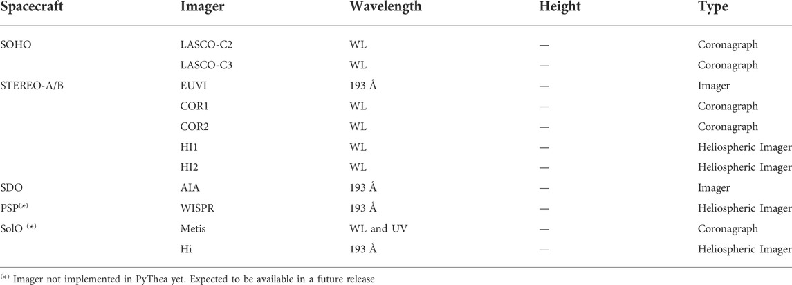
TABLE 1. A list of the available imagers used in PyThea.

For the selected imagers, Fido searches in VSO for available imaging data and retrieves them automatically. The search is performed at a time interval which is by default 1 hour before and after a user-selected central time. The user can extend the time interval in which the search and download is performed. For every new search, a new data set is downloaded for each of the selected imagers only when the data do not yet exist in the local database. If PyThea‘s GUI is used for this process, the data update (download and preparation of images) is fully automatic. We discuss PyThea‘s GUI in more detail in Section 3.

To load FITS files, PyThea uses the sunpy.Map.Map class from SunPy‘s utilities. This class is another powerful feature provided by SunPy, which is used to load solar imaging data. During the loading process, the sunpy.Map.Map class detects automatically the file type and the associated instrument using information from the FITS header. It also uses the FITS header keywords to determine and interpret the coordinate system of the imaging data, and construct the map metadata. This class provides the functionality needed to create a World Coordinate System (WCS) header from a SkyCoord object and the utilities to perform geometric transformations between different coordinate systems using the WCS interface (e.g. pixel_to_worldand world_to_pixel).

2.3 Imaging processing and visualization

PyThea provides general functions that can be used to filter and prepare the loaded maps (sunpy.map) before visualizing them. The first and most important aspect is to keep the images that meet certain criteria. Filtering the maps helps to load only those images whose quality is the best and can be used for the analysis. These functions remove duplicate images, or images with selected exposure times, dimensions, or polarization angles as far as the coronagraphic images are concerned. The final list of maps is returned as a sunpy.map.MapSequence, which is a chronologically ordered list.

The second set of functions can be used to prepare the images. This is a basic image processing step that includes four basic preparations: 1) normalization of the exposure time, 2) resampling of the images, and in the case of coronagraphic images, 3) masking the occulter and 4) combining different polarized brightness images that belong to the same polarization sequence. Most of the coronagraphic data are provided as total brightness images, except for STEREO/COR1, which are triplets of polarized brightness images in three different angles. Currently, PyThea (v0.6.6) does not include or provide the functionality to reprocess the FITS files and increase their processing level, e.g. to calibrate the images into physical units or to apply flat field corrections, remove stray light, correct geometric distortion and vignetting, and other corrections. However, the level of the FITS files provided from VSO is adequate to robustly perform the 3D reconstruction. The images are resampled with the use of the superpixel method that is provided by sunpy.map. This method reduces the resolution of the images by combining pixels and thus increasing the signal-to-noise ratio (SNR). The default image size used in PyThea is 512 × 512 pixels, providing fast processing times in the GUI and high SNR, which are essential to track the evolution of faint transients in the corona. The user can change the default image size for every imager separately by changing the configuration file. Additionally, during the processing of the coronagraphic images, we mask out the pixels that are inside the occulting disk since they do not contain any useful data.

During the geometrical fitting process, it is useful to use base or running difference images because it is easier to track the evolution of the CME and shock wavefront. Therefore, a final step of processing is to produce the base difference or running difference images from the plain images by subtracting the previous image or the first image in a sequence, respectively. PyThea provides utilities that can be used to process the images into base or running difference images, and returns the final maps as sunpy.map.MapSequence.

The final maps are plotted as images using the sunpy.map plot function. This function plots the map object using a method equivalent to imshow from matplotlib package (Hunter, 2007) and uses the “nearest neighbor” interpolation method. For plain images, we use false colours to better visualize them. SunPy provides the colourmap for each imager as defined by the instrument teams. For the difference images, we use a reverse grey colourmap and a linear normalization of the data. In Figure 2, we show an example of the images in EUV and WL produced with PyThea. The GCS (green grid in Figure 2) and ellipsoid geometrical model (red grid in Figure 2) are fitted to the CME and the shock wave, respectively, and overlaid to the images.

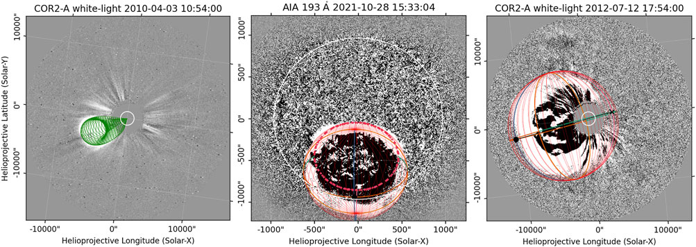
FIGURE 2. Running difference images in WL (right and left panels) and EUV (middle panel) produced with PyThea. The GCS (green grid), ellipsoid and spheroid models (red grid) are overplotted to the images.

2.4 The geometrical models

2.4.1 Overview

The fitting of the geometrical models to the observations is performed using near simultaneous images from multiple viewpoints. The final fit is registered to one of the selected images, hence, we term this as “single frame” fitting. Every single frame fitting can be converted into a pandas.DataFrame, which is a data structure, organizing them into a table row. This row contains the geometrical parameter values, the observation time of the image, and the source of the observations for only one fit. The different single frame fittings can be combined into a single table that constitutes the “event model fittings”, as we term this. The event model fittings is also a pandas.DataFrame containing information of the same geometrical parameters as the single frame fitting. The format of the event model fittings is similar to a spreadsheet, and it can be used to calculate the kinematics and to store the geometrical fitting to a file.

Each geometrical model is constructed as a class so that the user can create an object for each model. The models are described by a set of positional and geometrical parameters. The positional parameters are represented by using astropy.SkyCoord in the heliographic Stonyhurst (HGS) or heliographic Carrington (HGC) coordinate system. The origin of both coordinate systems is located at the solar center. The geometrical parameters of every model are described as physical quantities using astropy.units. Additionally, for each model we provide a method that returns the coordinates of the mesh points constructing the model. The points are represented using astropy.SkyCoord in the HGS frame.

2.4.2 The spheroid and ellipsoid model

The ellipsoid or spheroid models are usually used to reconstruct shock waves in 3D. CME-driven shock waves in the corona can be observed as propagating fronts in WL (e.g. Kwon et al., 2013). These fronts has been suggested to form the halo envelope of CMEs (Kwon et al., 2014), so that the outermost halo front part of the CMEs is formed by the propagating shock wave rather than a projection of the CME ejecta. In coronagraphic observations the projection of the large-scale morphology of the WL shock waves is usually seen as an ellipse. In 3D, the ellipsoid model seems a rather good approximation to describe the global large-scale structure of the WL shocks. Additionally, a simpler spheroid model can also be used, when it is better to perform the fitting with a reduced complexity.

First, we start from the definition of the ellipsoid model, which is the most generic case. An ellipsoid is a quadratic closed surface in which all plane cross-sections are either ellipses or circles. It has three mutually perpendicular axes of symmetry that intersect at a center of symmetry, which we will call hereafter the center of the ellipsoid. The three line segments along the axis of symmetry that start from the center of the ellipsoid and end at its surface are called the principal semi-axes of the ellipsoid, and they correspond to the semi-major axis and semi-minor axis of the plane cross-section ellipses.

The implicit equation of an ellipsoid in the Cartesian coordinate system is x²/a² + y²/b² + z²/c² = 1, where a, b, and c are the lengths of the three principal semi-axes. In Figure 3, we show an ellipsoid with the three axes of symmetry and the three principal semi-axes. In the case where the three semi-axes of the ellipsoid are equal (a = b = c), the surface is a sphere, and if only two semi-axes are equal, the surface is an ellipsoid of revolution, or most commonly called a spheroid. The two cases are also presented in Figure 3. Then, a spheroid is obtained by revolving an ellipse about one of its principal axes, and it has a circular symmetry. When revolving the ellipse about its minor (major) axis, an oblate (prolate) spheroid is formed. Therefore, a spheroid is oblate (prolate) when a and b are equal and also are greater (smaller) than c.

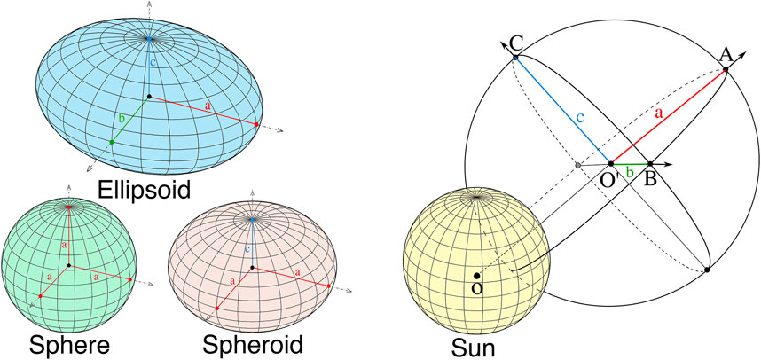
FIGURE 3. A schematic of three different ellipsoids (left), and of an ellipsoid model showing the different axis and parameters (right).

Since the spheroid is a special case of the ellipsoid model, we start by defining the latter first. To define the ellipsoid model, we use three positional and three geometrical parameters. In Table 2, we present synoptically the parameters for each model. The point of reference for the ellipsoid (and spheroid) model is the center of symmetry. In PyThea, this point is represented as a SkyCoord in the HGS coordinate system. In the spherical coordinates, the three positional parameters, r_center, ϕ, θ, define the heliocentric distance, latitude, and longitude of the ellipsoid center, respectively. Additionally, we define the primary (first) semi-axis of the ellipsoid model to start from the ellipsoid center and pointing radially outward towards the same direction as the position vector of the ellipsoid center. The other two semi-axis are orthogonal to the primary semi-axis, and their direction depends on the tilt angle, γ, relative to the solar equator. For γ = 0, one of the semi-axis is coplanar with the solar rotation vector, and the other semi-axis is parallel to the solar equatorial plane. Note that for the spheroid model the tilt angle is not defined since any rotation along the radial semi-axis is trivial as there is a circular symmetry with respect to this axis.

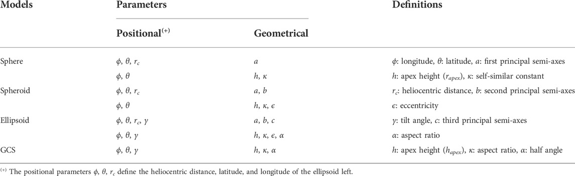
TABLE 2. Geometrical models available in PyThea showing the different parameters used.

The geometrical parameters of the ellipsoid model are the lengths a, b, and c of the three principal semi-axes (two in the case of the spheroid), respectively. The positional and geometrical parameters are sufficient to fully define the geometry of the ellipsoid model in 3D. PyThea‘s users can adjust the ϕ, θ, and γ values to match the position and orientation of the ellipsoid with the observed shock in WL and EUV, and the length of the three principal semi-axes to fit the geometry of the shock front in every direction. The ellipsoid model can also be constrained to expand self-similarly. This provides a more convenient way to perform the shock fittings. In this case, the positional and geometrical parameters have to be defined differently. Instead of using the length of the three semi-axes as the geometrical parameters, the user adjust the heliocentric height of the ellipsoid at the apex, and the length of the other two semi-axis are calculated using a self-similar constant (κ), an aspect ratio (α), and the eccentricity (ϵ) of the ellipsoid defined from the cross-sectional ellipse of two semi-axis. The κ parameter is a self-similar constant that is defined as the ratio of the height of the apex to the length of one of the semi-axis (κ = b/(r_apex − 1 R_⊙)). This value is proportional to the aspect ratio between the two semi-axis a and b. The OA line segment shown in Figure 3, is the height of the apex, so r_apex = OA = r_center + a. The α parameter is the second aspect ratio of the ellipsoid, and it is defined as α = b/c, while ϵ is the eccentricity, and we define it as follows:

In this case, users can adjust any of these four geometrical parameters r_apex, κ, α, and ϵ to fit the ellipsoid model to the observed shock front. Changing r_apex and keeping constant the other parameters, the expansion is self-similar. For the positional parameters, ϕ, θ, γ are also adjusted by the user, while r_center is calculated from r_center = r_apex − a.

2.4.3 The GCS model

The GCS model is an empirical geometrical model of a flux rope defined by Thernisien et al. (2006); Thernisien (2011). It consists of a curved front that is a cylindrical shell forming the main part of the CME–from its “legs” to the apex–and two attached cones that correspond to the legs of the CME. The resulting shape is reminiscent of a croissant, as we show in Figure 4. The model is constrained to expand self-similarly, which it seems to be the case for most of the CMEs at heliocentric heights $>$10 R_⊙ (e.g. Balmaceda et al., 2020). Previous studies (Dumbović et al., 2019) have shown that the GCS model reproduces well the large-scale structure of flux rope-like CMEs in the solar corona, and it is widely used to reconstruct their 3D structure.

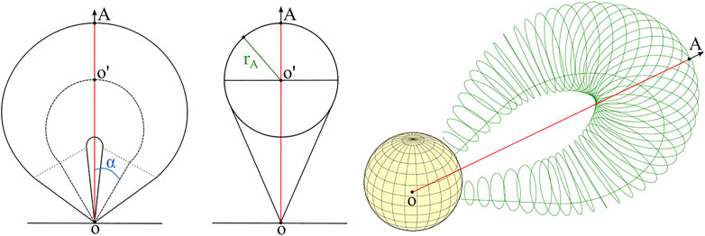
FIGURE 4. Plane sections of the GCS model (left and middle panels) showing the different parameters, and a schematic of the model mesh (right panel).

Following Thernisien et al. (2006), we define the GCS model using three positional and three geometrical parameters. These are given in Table 2. We define as a point of reference for the GCS model the apex center (A in Figure 4). This point is represented in PyThea as a SkyCoord in the HGS coordinate system. The primary axis of the GCS model is defined from the solar center and directed towards the apex center. In the spherical coordinates, the three positional parameters (r_apex, ϕ, θ) define the heliocentric distance, latitude, and longitude of the flux rope apex center, respectively. Additionally, the flux rope can be tilted relative to the solar equator. For a tilt angle, γ, equal to zero, both legs of the CME are located at the solar equator.

The geometrical parameters of the GCS model are three: 1) the heliocentric height at the apex, h_apex (OA in Figure 4), 2) the aspect ratio at the apex, κ, which is defined as the ratio OO’ to r_A and sets the rate of lateral versus radial expansion of the CME, and 3) the half angle, α, which is the angle between the axis of the cone and the primary axis. From these six parameters we can fully define the GCS model, therefore, in PyThea the user can adjust ϕ, θ, and γ to match the flux rope position and orientation with observations, and h_apex, κ, and α to fit the geometry.

2.5 Visualizing the geometrical models

To fit the geometrical models to the observed CMEs and shocks, the mesh points constructing the models, have to be projected to the respective images that are used for the reconstruction. For each geometrical model, the coordinates of the mesh points are represented using astropy.SkyCoord in the HGS frame so these points are in world coordinates. To visualize the mesh points we use SunPy functionality and plot_coord which plots an astropy.SkyCoord onto the image (see also astropy.plot_coord). The plot_coord method converts the world coordinates to pixel coordinates and plots them onto the images. The world-to-pixel coordinate transformation is based on the FITS WCS standard. This standard describes the geometric transformations between two sets of coordinates, hence, associating physical values to positions within the FITS dataset. In our case, the FITS WCS standard is used to convert the heliospheric coordinates to pixel coordinates of an image. SunPy supports a broad set of heliospheric coordinate systems (see Thompson, 2006) that extend the Astropy coordinates framework and also allows transformations between the different coordinate systems implemented in both SunPy and Astropy . The accuracy of the coordinate transformations and projections is a critical aspect that ultimately controls the accuracy of this software package. Thankfully, the functionality provided by the SunPy has been extensively tested and agrees with great accuracy with published values in the Astronomical Almanac. In Figure 5, we show two examples of the geometrical fitting to bodies in the Solar System with known locations and dimensions. This fitting provides a good test of the accuracy of the geometrical models and the coordinate transformations and the final visualization. For example, in Panel a, we show the Venus transit on 6 June 2012, as viewed by AIA at 19.3 nm. Using the location and radius of the planet we fit the ellipsoid model to Venus and visualize the result. To calculate the planet’s location, we used the Solar System ephemeris file (DE432s.bsp) provided by Jet Propulsion Laboratory and for the radius, we used the mean equatorial radius (R_V = 6051.8 km) provided by NASA’s space science data coordinated archive. The resulting fitting match very well with the observations. For Panel b, we used the same method for the Mercury transit on 9 May 2016, as viewed by AIA at 19.3 nm.

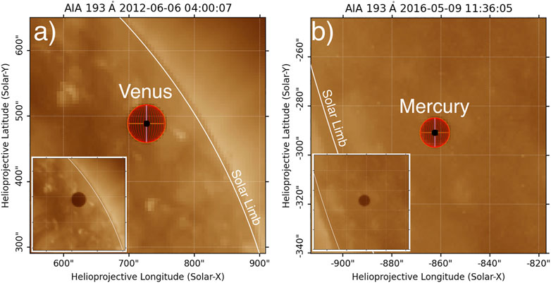
FIGURE 5. Two examples of the geometrical fitting to bodies in the solar system with known locations and dimensions. Panel (A) shows the Venus transit on 6 June 2012, and Panel (B) the Mercury transit on 9 May 2016, as viewed by AIA at 19.3 nm. The fitted ellipsoid to the planets is shown with the red mesh. The insert images show the AIA observations without the fitting.

2.6 Fittings processing and kinematic plots

The main goal when performing the geometrical 3D fitting of a CME or a shock wave is to reconstruct their 3D structure and determine their position and kinematics with accuracy, minimizing the projection effects. PyThea provides utility functions to further process the produced geometrical 3D fittings. These functions can be used to calculate the kinematics and visualize the temporal evolution of the fitted geometrical parameters.

Using PyThea‘s utilities, the user can perform a polynomial or spline fitting to the kinematic curves and determine the propagation and expansion speed. For the polynomial fitting, we use the numpy.polyfit function that performs a least squares polynomial fit of any degree to the set of data points. For the spline fit, we use the UnivariateSpline from the scipy.interpolate package (Virtanen et al., 2020). The user can change the degree of the smoothing spline (from unity to five) and the smoothing factor. The uncertainty of the kinematic is computed by the goodness of fit to the height-time data. For both fitting models, the uncertainty is calculated from the standard deviation. To calculate this for the polynomial method, we use the covariance matrix, whereas, for the spline fit it is computed from the residuals of the fit, which is a measure of how well a spline fits the data. An example of the produced height (length)-time and speed-time plots is given in Figure 8 where we perform a full reconstruction for a solar event.

2.7 Save/load the fitting results

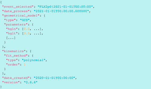
The results of the geometrical 3D fittings can be saved and then loaded again to preview or continue the analysis for an event. As we mentioned in Section 2.4.1, the individual frame fittings are stored in the model_fittings class that initializes an object to store all the frame fittings of the geometrical model. This object contains two methods, to_dict() and to_json(), that can be used to return the final fittings of the geometrical model in either a dictionary or JSON (JavaScript Object Notation) file format. JSON is an open, language-independent standard file format, that uses human-readable text to store data in attribute–value pair format. In Python, the JSON files can be easily imported and converted into a dictionary using the JSON encoder and decoder package. Inside the JSON file, we store information about the date and time of the selected event, the geometrical model used and the parameters of the geometrical model, which is a pandas.DataFrame of the frame fittings, and the parameters used to process the kinematics, that is the selected fitting method and the associated fitting parameters. An example of the exported JSON file is given below:

Listing 1: An example of the exported JSON file.

3 The web application

3.1 Graphical user interface

Performing a 3D reconstruction is mainly an interactive process. To reconstruct an event, the user aim to achieve the best fit of a geometrical model to multi-viewpoint coronal observations by adjusting a set of geometrical parameters. Without a GUI, this process is almost impossible to be performed. For that reason, in PyThea we provide a modern application that can be used to perform a full analysis of an event. The GUI of this application has been built based on Streamlit. Figure 6 shows two views of the PyThea‘s web application. Panel a shows the starting page of PyThea and panel b the main fitting page. The web app consists of two main vertical panels, panels 1 and 2 as labeled in Figure 6. Panel one is used as a placeholder for the user input widgets, while panel two is used for the display of data elements. Additionally, in Figure 7 we show a more detailed view of the four input widgets contained in panel 1.

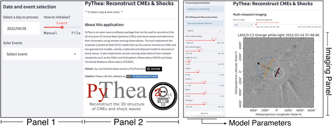
FIGURE 6. Two views of PyThea‘s web application. The left panel shows the starting page of the application and the right panel shows the main fitting page.

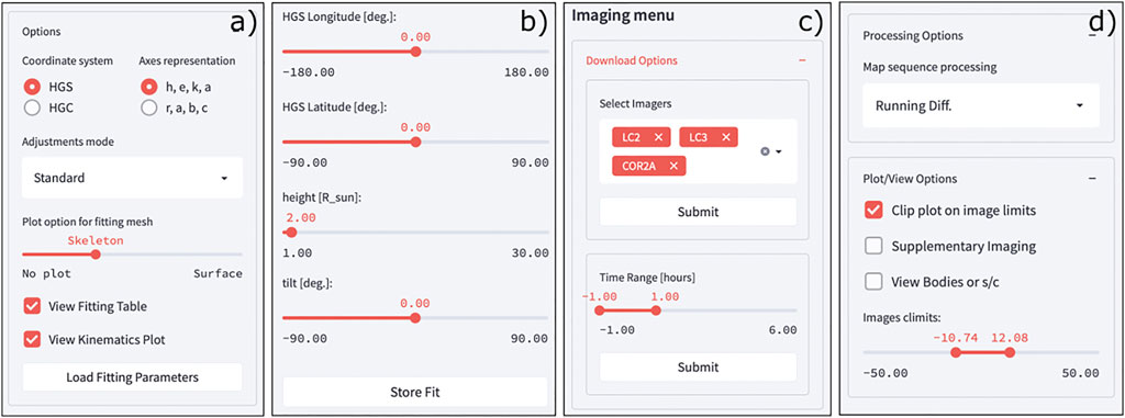
FIGURE 7. Panels (A–D) show a detailed view of the panels that appear in PyThea‘s web application. These panels contain the different input widgets such as sliders, radio buttons, drop boxes, and others that can be used to provide input parameters to the application.

3.2 Initializing the fitting process

When the web application starts for the first time, the user has to initialize it by choosing one of three different options. The first option is to select the date of the fitting. After this selection, the application searches in the Heliophysics Events Knowledgebase (HEK: Hurlburt et al., 2010) database for registered solar flares and returns them in a dropdown menu. Each option contains information about the flare class and the flare maximum time, and the user can select among the different events. This selection is used to associate the fitting to a flare and give a unique identification label to the final products. The identification label is used mainly for archiving purposes of the final fitting files. If the user does not want to associate the fitting files to a flare or when a solar flare has not been registered in the HEK database at the time of the CME or the shock under investigation (for example because the flare was located behind the visible disk), the user can select the second option which is to initialize the application manually. This is dome by choosing between different event identification labels (e.g. CME, shock) and select manually the date and time of the solar event under investigation to start the fitting process. The next step is the selection of the geometrical model (i.e. the ellipsoid) that is used for the fitting. After this step, the application is ready to initiate, and the data download and loading process starts. We give further details of this process below. The third option is to provide a fitting file previously processed and the application will automatically initialize. Then the fitting file loads the user can preview or continue the fitting process.

3.3 Imaging data download, load, and process

The application downloads, loads, and processes the imaging data automatically after the selection of the geometrical model. By default only three imagers are loaded in the beginning, however, more instruments can be selected from a list of supported imagers (see Figure 7C, top) incide the application. The application searches in VSO for available imaging data for a selected time interval before and after the event’s characteristic time (i.e. the flare maximum). This time interval can be changed during the fitting process (see Figure 7C, bottom). When a new imager is selected or when the time interval changes, the application automatically downloads and processes the new images. The imaging data are displayed in the “Image Panel” shown in Figure 6B. By default the images are processed as running difference images. The application provides also the option to view base difference or plain images (see Figure 7D, top). The main imager of which the data is viewed on the main fitting page can be selected from a dropdown menu. An example is shown in Figure 6B. Using a time slider, the different loaded images can be viewed.

3.4 The geometrical fitting process

At every image the geometrical model is over-plotted with or without the grid of the fitting mesh. The parameters of the geometrical model can be changed by adjusting the parameter sliders (see Figure 7B). Any update of the model parameters results in an automatic update of the location of the model in the images. The fitting process is repeated until there is a good fit of the geometrical model to the observations. For the multi-viewpoint analysis of an event, nearly-simultaneous images from at least three different imagers have to be used and the geometrical model has to have a good fit in more than one image. To perform a multi-viewpoint fitting the application provides two supplementary images that appear on two side-by-side panels below the primary image that is already displayed on the top. The data from the supplementary imagers are the closest in time available images to the main image.

The geometrical fitting to a single image (or triplet of images) can be saved and every new single frame fitting is added to a pandas.DataFrame, which can be used to construct the model_fittings object. This object contains all the information about the geometrical fitting process and is used to export the final results to a JSON file format (see Section 2.7). Additionally, single frame fitting is uniquely stored in the pandas.DataFrame, so when the model parameters change the values in the table update automatically without registering a new record if this record already exists.

During the multiple-viewpoint, multiple-time, fitting process, PyThea provides two options to view and supervise the fitting parameters. The first enables a view of the fittings pandas.DataFrame table where the values of the geometrical model can be previewed. A single-frame fitting can be selected and loaded or deleted. When a single-frame fitting is loaded all the geometrical parameters are loaded to the sliders and the fitting can be revised. The second option enables the processing and visualization of kinematics. Various functions can be fitted in the height-time profiles of the CMEs and the shocks. The kinematic plots are displayed below the imaging panel in the application. These plots can be saved in PNG format during the fitting process. Additionally, the geometrical fittings can be downloaded as JSON files (see Section 2.7) at any time during the fitting process.

3.5 An example shock reconstruction

Using the web application of PyThea we reconstructed the solar event on 7 March 2012 and use this as an example of the product that can be produced with this software package and can lead to significant scientific discoveries as we explained in the Introduction. This solar event was associated with a powerful X5.4 class flare from AR 11429 that was located at N18°E31°. The flare started at 00:02 UT and peaked at 00:24 UT and was accompanied by a bright coronal EUV wave and an ultra-fast CME and a shock wave. The event was also associated with a major SEP event on the same day which was one of the strongest proton events of 2012 and was detected by three spacecraft separated at least 120° apart in longitude. This event has been analysed with great detail by previous studies (Kwon et al., 2014; Kouloumvakos et al., 2016) that showed that a very fast shock wave formed, capable to accelerate and release SEPs in very distant locations in the heliosphere.

In Figure 8, we show a few of the results from the shock reconstruction. Panels a) and b) show remote sensing observations from the two STEREO spacecraft. We project the reconstructed shock wave front onto the event images. For this reconstruction, there were available data from three different viewpoints, of STEREO-A/B and SOHO. The location of the spacecraft and Earth are shown in panel c) of Figure 8 where we show a view of the ecliptic plane from the ecliptic north. Panels d1) and d2), show the kinematic profiles of the shock wave. We have spline-fitted the height (length)-time measurement and then calculated the kinematic curves that are shown on panel d2), from the time derivative of the spline fit. For this calculation, we use the gradient of the height (length)-time measurements. The gradient is computed using a second-order central differences scheme in the interior points and a first-order one-side differences scheme at the boundaries. The derived kinematics agree well, within the uncertainties, with the shock speed values derived in previous studies. We find a maximum speed of $\sim 3270\pm$200 km/s at the shock apex, while from Figure 10 of Kwon et al. (2014) we estimate that the maximum shock speed is ∼3180 km/s. The two results seem to be in good agreement considering the inherent uncertainty of the fitting process which is user dependent and the uncertainty of the final fitting of the kinematics.

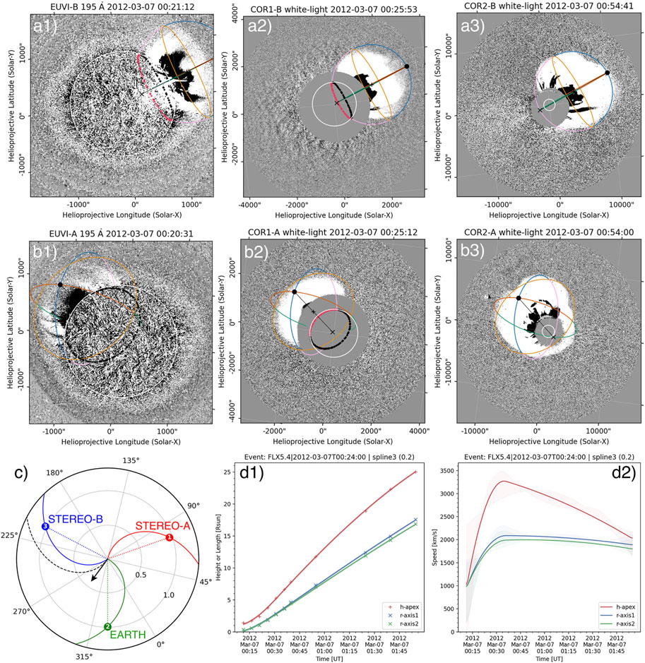
FIGURE 8. Selected results from the shock reconstruction of the 7 March 2012 solar event. Panels (A1–A3), show images from STEREO-A EUVI, COR1, and COR2 where we also show the reconstructed shock wave front. Similar to panels (B1–B3) that show nearly simultaneous images from STEREO-B. Panel (C) is a view of the ecliptic plane from the ecliptic north showing the relative positions of the STEREO-A/B and Earth in Carrington coordinates, on 7 March 2012 at 00:15 UT. This ecliptic view is produced with the Solar-MACH tool. Panels (D1, D2), show the height and kinematic time profile plots, respectively, of the reconstructed shock wave.

4 Discussion and future prospects

In this paper, we present PyThea to the scientific community, which is a newly developed open-source Python software package that provides tools to reconstruct CMEs and shock waves. This package has been fully built in Python, with extensive use of libraries available within this language ecosystem. We showed details of the main functionality of the core software package and also presented the web application that can be used to reconstruct CMEs and shocks waves with reduced complexity, especially in data retrieval and data reduction.

The current version of PyThea is v0.6.6 and can be installed using PyPI. The source code can also be found on GitHub and Zenodo⁶. The development of the PyThea core package has been ongoing for 1 year and uninterrupted since its first release. We hope the community appreciate this effort and that the number of users who explore the capabilities of PyThea keeps growing in the nearly future. We welcome any critical review that would make this package better for the community.

A significant milestone is to reach the standards of version 1.0.0 soon. This would require a higher level of documentation, with guidelines and tutorials and enhanced documentation strings of the functions and classes used in the core package. Additionally, increased coverage and a better level of testing of the various components of the package are necessary and automation of several processes such as doc build, testing, and packaging will be needed for the stable version. Lastly, finalizing the stability of the core package will assure that the minor releases are backwards compatible and that only major releases would have breaking changes or new major features.

Further development of this package to include imaging data from the two new solar missions, PSP and SolO, is considered to be a priority. Additionally, we plan to improve various current features and include new ones. The main focus will be to ease and improve, even further, the reconstruction process and enhance the visualization part. For example, we plan to include features that would allow the user to change the base difference images, select the step of the running difference images, zoom into the images, draw a grid over the solar surface or plot the solar limb visible from Earth perspective for different observers. Further developments in the image processing would also allow us to make the fitting process semi-automatic in future releases. These and other features will be considered in a future release. Currently, no funding is associated directly with the development of the package, however, we will pursue opportunities for financial support to continue maintaining and making significant contributions to PyThea.

Data availability statement

Publicly available datasets were analyzed in this study. The data can be accessed at the Virtual Solar Observatory (http://sdac.virtualsolar.org/cgi/search). These data were processed and analyzed using Python’s SunPy package (The SunPy Community et al., 2020).

Author contributions

AK developed PyThea software package. JG, LR-G, and DP have tested PyThea’s application and provided critical comments for the development and release of the package. AK prepared the first draft and all the authors involved in the preparation of the final manuscript and critically revised it. All authors have read the paper and approved its submission.

Funding

This study has received funding from the European Union’s Horizon 2020 research and innovation programme under grant agreement No. 101004159 (SERPENTINE). AK acknowledges financial support from the SERPENTINE project that allowed to initiate PyThea’s development and from NASA NNN06AA01C (SO-SIS Phase-E) contract that allowed further improvements and update of the package to the version used for this study. LR-G acknowledges the financial support by the Spanish Ministerio de Ciencia, Innovación y Universidades FEDER/MCIU/AEI Projects ESP2017-88436-R and PID2019-104863RB-I00/AEI/10.13039/501100011033. JG and RV acknowledge the support of Academy of Finland (FORESAIL, grants 312357 and 336809). AV was supported by NASA 80NSSC19K1261 and LWS 80NSSC19K0069 grants.

Acknowledgments

This research has made use of PyThea v0.6.6, an open-source and free Python package to reconstruct the 3D structure of CMEs and shock waves (Zenodo: https://doi.org/10.5281/zenodo.5713659). This research used version 4.0.0 of the SunPy open source software package (The SunPy Community et al., 2020). The Solar-MACH tool was originally developed at Kiel University, Germany and further discussed within the ESA Heliophysics Archives USer (HAUS) group. SOHO is an international collaboration between NASA and ESA. LASCO was constructed by a consortium of institutions: NRL (United States), MPIA (Germany), LAS (France), and the University of Birmingham (UK). The SECCHI data are produced by an international consortium of the NRL, LMSAL and NASA GSFC (United States), RAL and the University of Birmingham (UK), MPS (Germany), CSL (Belgium), IOTA and IAS (France). The AIA data used here are courtesy of SDO (NASA) and the AIA consortium. We thank the AIA team for easy access to calibrated data.

Conflict of interest

The authors declare that the research was conducted in the absence of any commercial or financial relationships that could be construed as a potential conflict of interest.

Publisher’s note

All claims expressed in this article are solely those of the authors and do not necessarily represent those of their affiliated organizations, or those of the publisher, the editors and the reviewers. Any product that may be evaluated in this article, or claim that may be made by its manufacturer, is not guaranteed or endorsed by the publisher.

Footnotes

¹https://github.com/AthKouloumvakos/PyThea

²GNU General Public License v3.0

³Python has overtaken C at 1st position in October 2021 in TIOBE Programming Community index. This index is an indicator of the popularity of programming languages.

⁴https://pypi.org/project/PyThea/

⁵More details of how to manage environments using conda are provided in this link

⁶Zenodo is a general-purpose open repository developed under the European OpenAIRE program and is powered by CERN Data Centre.

References

Balmaceda, L. A., Vourlidas, A., Stenborg, G., and Cyr, St.O. C. (2020). On the expansion speed of coronal mass ejections: Implications for self-similar evolution. Sol. Phys.295, 107. doi:10.1007/s11207-020-01672-6
Balmaceda, L. A., Vourlidas, A., Stenborg, G., and Kwon, R.-Y. (2022). The hyper-inflation stage in the coronal mass ejection formation: A missing link that connects flares, coronal mass ejections, and shocks in the low corona. Astrophys. J.931, 141. doi:10.3847/1538-4357/ac695c
The SunPy Community, Barnes, W. T., Bobra, M. G., Christe, S. D., Freij, N., Hayes, L. A., et al. (2020). The sunpy project: Open source development and status of the version 1.0 core package. Astrophys. J.890, 68. doi:10.3847/1538-4357/ab4f7a
Chen, P. F. (2011). Coronal mass ejections: Models and their observational basis. Living Rev. Sol. Phys.8, 1. doi:10.12942/lrsp-2011-1
Domingo, V., Fleck, B., and Poland, A. I. (1995). The SOHO mission: An overview. Sol. Phys.162, 1–37. doi:10.1007/BF00733425
Dresing, N., Kouloumvakos, A., Vainio, R., and Rouillard, A. (2022). On the role of coronal shocks for accelerating solar energetic electrons. Astrophys. J. Lett.925, L21. doi:10.3847/2041-8213/ac4ca7
Dumbović, M., Guo, J., Temmer, M., Mays, M. L., Veronig, A., Heinemann, S. G., et al. (2019). Unusual plasma and particle signatures at mars and STEREO-A related to CME-CME interaction. Astrophys. J.880, 18. doi:10.3847/1538-4357/ab27ca
Fox, N. J., Velli, M. C., Bale, S. D., Decker, R., Driesman, A., Howard, R. A., et al. (2016). The solar Probe plus mission: Humanity’s first visit to our star. Space Sci. Rev.204, 7–48. doi:10.1007/s11214-015-0211-6
Frassati, F., Susino, R., Mancuso, S., and Bemporad, A. (2019). Comprehensive analysis of the formation of a shock wave associated with a coronal mass ejection. Astrophys. J.871, 212. doi:10.3847/1538-4357/aaf9af
Giacalone, J., Mitchell, D. G., Allen, R. C., Hill, M. E., and McNutt, J. (2020). Solar Energetic Particles Produced by a Slow Coronal Mass Ejection at ∼0.25 au. Astrophys. J. Suppl. Ser.246, 29. doi:10.3847/1538-4365/ab5221
Gómez-Herrero, R., Dresing, N., Klassen, A., Heber, B., Lario, D., Agueda, N., et al. (2015). Circumsolar energetic particle distribution on 2011 november 3. Astrophys. J.799, 55. doi:10.1088/0004-637x/799/1/55
Harris, C. R., Millman, K. J., van der Walt, S. J., Gommers, R., Virtanen, P., Cournapeau, D., et al. (2020). Array programming with NumPy. Nature585, 357–362. doi:10.1038/s41586-020-2649-2
Hess, P., Rouillard, A. P., Kouloumvakos, A., Liewer, P. C., Zhang, J., Dhakal, S., et al. (2020). WISPR imaging of a pristine CME. Astrophys. J. Suppl. Ser.246, 25. doi:10.3847/1538-4365/ab4ff0
Howard, R. A., Moses, J. D., Vourlidas, A., Newmark, J. S., Socker, D. G., Plunkett, S. P., et al. (2008). Sun Earth connection coronal and heliospheric investigation (SECCHI). Space Sci. Rev.136, 67–115. doi:10.1007/s11214-008-9341-4
Hunter, J. D. (2007). Matplotlib: A 2d graphics environment. Comput. Sci. Eng.9, 90–95. doi:10.1109/MCSE.2007.55
Hurlburt, N. E., Cheung, M., Schrijver, C., Chang, L., Freeland, S., Green, S., et al. (2010). An introduction to the heliophysics event Knowledgebase. Am. Astronomical Soc. Meet. Abstr. #216216, 40222.
Jebaraj, I. C., Kouloumvakos, A., Magdalenic, J., Rouillard, A. P., Mann, G., Krupar, V., et al. (2021). Generation of interplanetary type II radio emission. Astron. Astrophys.654, A64. doi:10.1051/0004-6361/202141695
Kaiser, M. L., Kucera, T. A., Davila, J. M., Cyr, St.O. C., Guhathakurta, M., and Christian, E. (2008). The STEREO mission: An introduction. Space Sci. Rev.136, 5–16. doi:10.1007/s11214-007-9277-0
Kouloumvakos, A., Kwon, R. Y., Rodríguez-García, L., Lario, D., Dresing, N., Kilpua, E. K. J., et al. (2022). The first widespread solar energetic particle event of solar cycle 25 on 2020 November 29. Shock wave properties and the wide distribution of solar energetic particles. Astron. Astrophys.660, A84. doi:10.1051/0004-6361/202142515
Kouloumvakos, A., Patsourakos, S., Nindos, A., Vourlidas, A., Anastasiadis, A., Hillaris, A., et al. (2016). Multi-viewpoint observations of a widely distributed solar energetic particle event: The role of EUV waves and white-light shock signatures. Astrophys. J.821, 31. doi:10.3847/0004-637X/821/1/31
Kouloumvakos, A., Rouillard, A. P., Share, G. H., Plotnikov, I., Murphy, R., Papaioannou, A., et al. (2020a). Evidence for a coronal shock wave origin for relativistic protons producing solar gamma-rays and observed by neutron monitors at Earth. Astrophys. J.893, 76. doi:10.3847/1538-4357/ab8227
Kouloumvakos, A., Rouillard, A. P., Wu, Y., Vainio, R., Vourlidas, A., Plotnikov, I., et al. (2019). Connecting the properties of coronal shock waves with those of solar energetic particles. Astrophys. J.876, 80. doi:10.3847/1538-4357/ab15d7
Kouloumvakos, A., Rouillard, A., Warmuth, A., Magdalenic, J., Jebaraj, I. C., Mann, G., et al. (2021). Coronal conditions for the occurrence of type II radio bursts. Astrophys. J.913, 99. doi:10.3847/1538-4357/abf435
Kouloumvakos, A., Vourlidas, A., Rouillard, A. P., Roelof, E. C., Leske, R., Pinto, R., et al. (2020b). The solar origin of particle events measured by parker solar Probe. Astrophys. J.899, 107. doi:10.3847/1538-4357/aba5a1
Kwon, R.-Y., Ofman, L., Olmedo, O., Kramar, M., Davila, J. M., Thompson, B. J., et al. (2013). STEREO observations of fast magnetosonic waves in the extended solar corona associated with EIT/EUV waves. Astrophys. J.766, 55. doi:10.1088/0004-637X/766/1/55
Kwon, R.-Y., and Vourlidas, A. (2017). Investigating the wave nature of the outer envelope of halo coronal mass ejections. Astrophys. J.836, 246. doi:10.3847/1538-4357/aa5b92
Kwon, R.-Y., Zhang, J., and Olmedo, O. (2014). New insights into the physical nature of coronal mass ejections and associated shock waves within the framework of the three-dimensional structure. Astrophys. J.794, 148. doi:10.1088/0004-637X/794/2/148
Lakhina, G. S., and Tsurutani, B. T. (2016). Geomagnetic storms: Historical perspective to modern view. Geosci. Lett.3, 5. doi:10.1186/s40562-016-0037-4
Lario, D., Kwon, R. Y., Richardson, I. G., Raouafi, N. E., Thompson, B. J., von Rosenvinge, T. T., et al. (2017). The solar energetic particle event of 2010 august 14: Connectivity with the solar source inferred from multiple spacecraft observations and modeling. Astrophys. J.838, 51. doi:10.3847/1538-4357/aa63e4
Lario, D., Kwon, R. Y., Vourlidas, A., Raouafi, N. E., Haggerty, D. K., Ho, G. C., et al. (2016). Longitudinal properties of a widespread solar energetic particle event on 2014 february 25: Evolution of the associated CME shock. Astrophys. J.819, 72. doi:10.3847/0004-637X/819/1/72
Lario, D., Raouafi, N. E., Kwon, R. Y., Zhang, J., Gómez-Herrero, R., Dresing, N., et al. (2014). The solar energetic particle event on 2013 april 11: An investigation of its solar origin and longitudinal spread. Astrophys. J.797, 8. doi:10.1088/0004-637X/797/1/8
Long, D. M., Bloomfield, D. S., Chen, P. F., Downs, C., Gallagher, P. T., Kwon, R. Y., et al. (2017). Understanding the physical nature of coronal “EIT waves”. Sol. Phys.292, 7. doi:10.1007/s11207-016-1030-y
Mancuso, S., Frassati, F., Bemporad, A., and Barghini, D. (2019). Three-dimensional reconstruction of CME-driven shock-streamer interaction from radio and EUV observations: A different take on the diagnostics of coronal magnetic fields. Astron. Astrophys.624, L2. doi:10.1051/0004-6361/201935157
Mierla, M., Inhester, B., Antunes, A., Boursier, Y., Byrne, J. P., Colaninno, R., et al. (2010). On the 3-D reconstruction of Coronal Mass Ejections using coronagraph data. Ann. Geophys.28, 203–215. doi:10.5194/angeo-28-203-2010
Morosan, D. E., Palmerio, E., Pomoell, J., Vainio, R., Palmroth, M., and Kilpua, E. K. J. (2020). Three-dimensional reconstruction of multiple particle acceleration regions during a coronal mass ejection. Astron. Astrophys.635, A62. doi:10.1051/0004-6361/201937133
Müller, D., Cyr, St.O. C., Zouganelis, I., Gilbert, H. R., Marsden, R., Nieves-Chinchilla, T., et al. (2020). The Solar Orbiter mission. Science overview. Astron. Astrophys.642, A1. doi:10.1051/0004-6361/202038467
Mumford, S., Freij, N., Christe, S., Ireland, J., Mayer, F., Hughitt, V., et al. (2020). Sunpy: A python package for solar physics. J. Open Source Softw.5, 1832. doi:10.21105/joss.01832
Ontiveros, V., and Vourlidas, A. (2009). Quantitative measurements of coronal mass ejection-driven shocks from LASCO observations. Astrophys. J.693, 267–275. doi:10.1088/0004-637X/693/1/267
Palmerio, E., Nieves-Chinchilla, T., Kilpua, E. K. J., Barnes, D., Zhukov, A. N., Jian, L. K., et al. (2021). Magnetic structure and propagation of two interacting CMEs from the Sun to saturn. J. Geophys. Res. Space Phys.126, e2021JA029770. doi:10.1029/2021JA029770
Patsourakos, S., and Vourlidas, A. (2012). On the nature and genesis of EUV waves: A synthesis of observations from SOHO, STEREO, SDO, and hinode (invited review). Sol. Phys.281, 187–222. doi:10.1007/s11207-012-9988-6
Pesnell, W. D., Thompson, B. J., and Chamberlin, P. C. (2012). The solar Dynamics observatory (SDO). Sol. Phys.275, 3–15. doi:10.1007/s11207-011-9841-3
Astropy Collaboration, Price-Whelan, A. M., Sipőcz, B. M., Günther, H. M., Lim, P. L., Crawford, S. M., et al. (2018). The astropy project: Building an open-science project and status of the v2.0 core package. Astron. J.156, 123. doi:10.3847/1538-3881/aabc4f
Astropy Collaboration, Robitaille, T. P., Tollerud, E. J., Greenfield, P., Droettboom, M., Bray, E., et al. (2013). Astropy: A community Python package for astronomy. Astron. Astrophys.558, A33. doi:10.1051/0004-6361/201322068
Rodríguez-García, L., Gómez-Herrero, R., Zouganelis, I., Balmaceda, L., Nieves-Chinchilla, T., Dresing, N., et al. (2021). The unusual widespread solar energetic particle event on 2013 August 19. Solar origin and particle longitudinal distribution. Astron. Astrophys.653, A137. doi:10.1051/0004-6361/202039960
Rodríguez-García, L., Nieves-Chinchilla, T., Gómez-Herrero, R., Zouganelis, I., Vourlidas, A., Balmaceda, L. A., et al. (2022). Evidence of a complex structure within the 2013 august 19 coronal mass ejection - radial and longitudinal evolution in the inner heliosphere. Astron. Astrophys.662, A45. doi:10.1051/0004-6361/202142966
Rouillard, A. P., Plotnikov, I., Pinto, R. F., Tirole, M., Lavarra, M., Zucca, P., et al. (2016). Deriving the properties of coronal pressure fronts in 3D: Application to the 2012 may 17 ground level enhancement. Astrophys. J.833, 45. doi:10.3847/1538-4357/833/1/45
Rouillard, A. P., Poirier, N., Lavarra, M., Bourdelle, A., Dalmasse, K., Kouloumvakos, A., et al. (2020). Modeling the early evolution of a slow coronal mass ejection imaged by the parker solar Probe. Astrophys. J. Suppl. Ser.246, 72. doi:10.3847/1538-4365/ab6610
Rouillard, A. P., Sheeley, N. R., Tylka, A., Vourlidas, A., Ng, C. K., Rakowski, C., et al. (2012). The longitudinal properties of a solar energetic particle event investigated using modern solar imaging. Astrophys. J.752, 44. doi:10.1088/0004-637X/752/1/44
Scolini, C., Chané, E., Temmer, M., Kilpua, E. K. J., Dissauer, K., Veronig, A. M., et al. (2020). CME-CME interactions as sources of CME geoeffectiveness: The formation of the complex ejecta and intense geomagnetic storm in 2017 early september. Astrophys. J. Suppl. Ser.247, 21. doi:10.3847/1538-4365/ab6216
Temmer, M. (2021). Space weather: The solar perspective. Living Rev. Sol. Phys.18, 4. doi:10.1007/s41116-021-00030-3
Thernisien, A. F. R., Howard, R. A., and Vourlidas, A. (2006). Modeling of flux rope coronal mass ejections. Astrophys. J.652, 763–773. doi:10.1086/508254
Thernisien, A. (2011). Implementation of the graduated cylindrical shell model for the three-dimensional reconstruction of coronal mass ejections. Astrophys. J. Suppl. Ser.194, 33. doi:10.1088/0067-0049/194/2/33
Thompson, W. T. (2006). Coordinate systems for solar image data. Astron. Astrophys.449, 791–803. doi:10.1051/0004-6361:20054262
Virtanen, P., Gommers, R., Oliphant, T. E., Haberland, M., Reddy, T., Cournapeau, D., et al. (2020). SciPy 1.0: Fundamental algorithms for scientific computing in Python. Nat. Methods17, 261–272. doi:10.1038/s41592-019-0686-2
Webb, D. F., and Howard, T. A. (2012). Coronal mass ejections: Observations. Living Rev. Sol. Phys.9, 3. doi:10.12942/lrsp-2012-3
Wood, B. E., Wu, C. C., Howard, R. A., Socker, D. G., and Rouillard, A. P. (2011). Empirical reconstruction and numerical modeling of the first geoeffective coronal mass ejection of solar cycle 24. Astrophys. J.729, 70. doi:10.1088/0004-637X/729/1/70
Zhu, B., Liu, Y. D., Kwon, R.-Y., and Wang, R. (2018). Investigation of energetic particle release using multi-point imaging and in situ observations. Astrophys. J.865, 138. doi:10.3847/1538-4357/aada80
Zouganelis, I., De Groof, A., Walsh, A. P., Williams, D. R., Müller, D., St Cyr, O. C., et al. (2020). The Solar Orbiter Science Activity Plan. Translating solar and heliospheric physics questions into action. Astron. Astrophys.642, A3. doi:10.1051/0004-6361/202038445
Keywords: heliophysics, python software package, solar corona, coronal mass ejection, shock wave, remote-sensing solar observations, 3D reconstruction
Citation: Kouloumvakos A, Rodríguez-García L, Gieseler J, Price DJ, Vourlidas A and Vainio R (2022) PyThea: An open-source software package to perform 3D reconstruction of coronal mass ejections and shock waves. Front. Astron. Space Sci. 9:974137. doi: 10.3389/fspas.2022.974137
Received: 20 June 2022; Accepted: 04 August 2022;
Published: 06 September 2022.
Edited by:
Angeline G. Burrell, United States Naval Research Laboratory, United StatesReviewed by:
Stefano Markidis, KTH Royal Institute of Technology, SwedenFeng Wang, Guangzhou University, China
Copyright © 2022 Kouloumvakos, Rodríguez-García, Gieseler, Price, Vourlidas and Vainio. This is an open-access article distributed under the terms of the Creative Commons Attribution License (CC BY). The use, distribution or reproduction in other forums is permitted, provided the original author(s) and the copyright owner(s) are credited and that the original publication in this journal is cited, in accordance with accepted academic practice. No use, distribution or reproduction is permitted which does not comply with these terms.
*Correspondence: Athanasios Kouloumvakos, Athanasios.Kouloumvakos@jhuapl.edu