


Abstract
We analyze one of the first solar energetic particle (SEP) events of solar cycle 24 observed at widely separated spacecraft in order to assess the reliability of models currently used to determine the connectivity between the sources of SEPs at the Sun and spacecraft in the inner heliosphere. This SEP event was observed on 2010 August 14 by near-Earth spacecraft, STEREO-A (∼80° west of Earth) and STEREO-B (∼72° east of Earth). In contrast to near-Earth spacecraft, the footpoints of the nominal magnetic field lines connecting STEREO-A and STEREO-B with the Sun were separated from the region where the parent fast halo coronal mass ejection (CME) originated by ∼88° and ∼47° in longitude, respectively. We discuss the properties of the phenomena associated with this solar eruption. Extreme ultraviolet and white-light images are used to specify the extent of the associated CME-driven coronal shock. We then assess whether the SEPs observed at the three heliospheric locations were accelerated by this shock or whether transport mechanisms in the corona and/or interplanetary space provide an alternative explanation for the arrival of particles at the poorly connected spacecraft. A possible scenario consistent with the observations indicates that the observation of SEPs at STEREO-B and near Earth resulted from particle injection by the CME shock onto the field lines connecting to these spacecraft, whereas SEPs reached STEREO-A mostly via cross-field diffusive transport processes. The successes, limitations, and uncertainties of the methods used to resolve the connection between the acceleration sites of SEPs and the spacecraft are evaluated.
Export citation and abstract BibTeX RIS
1. Introduction
The nearly simultaneous observation of solar energetic particle (SEP) events by spacecraft that are widely separated in heliolongitude has generated a number of explanations to account for the access of SEPs to extended regions of the heliosphere (e.g., Richardson et al. 2014; Gómez-Herrero et al. 2015, and references therein). For example, cross-field diffusion processes in either the solar corona and/or interplanetary (IP) space that allow particles injected from a narrow solar region to spread over a wide range of heliolongitudes have been proposed by some authors (e.g., Zhang et al. 2009 and references therein). Broad particle sources associated with coronal and interplanetary shocks initially driven by coronal mass ejections (CMEs) that accelerate and inject particles into extended regions of the heliosphere have also been proposed (e.g., Cliver et al. 1995). The near-simultaneous occurrences of widely separated solar eruptions, or complex magnetic field configurations in the corona or in IP space, have also been suggested as mechanisms to spread particles over wide regions of the inner heliosphere (e.g., Richardson et al. 1991; Klein et al. 2008; Masson et al. 2013; Schrijver et al. 2013).
In order to distinguish between these possible interpretations, and to quantify the contribution of each process if several occur, it is essential to (1) combine in situ and remote multi-spacecraft observations with models that allow the magnetic connection between spacecraft and particle sources to be estimated, and (2) investigate the transport processes that allow SEPs to reach each spacecraft. In this article, we present a comprehensive study of an SEP event that was observed at well-separated heliospheric longitudes by near-Earth spacecraft and by the two spacecraft of the Solar TErrestrial RElations Observatory (STEREO-A and STEREO-B). The study of this SEP event allows us to asses different methods commonly used by the heliospheric community to identify the putative sources of SEPs, determine the magnetic connectivity that is established between the spacecraft and these sources, and specify the mechanisms by which SEPs reach spacecraft located at different heliolongitudes. In particular, we evaluate several methods employed to determine (1) the magnetic connectivity between spacecraft in the inner heliosphere and the Sun, (2) the extent and speed of the shock associated with the parent CME, and (3) the release time of the SEPs observed at the onset of the event by the different spacecraft. These methods allow us to specify whether the estimated release times of the SEPs observed by each spacecraft are consistent with the times when each spacecraft established magnetic connection with the particle sources, identified as those portions of the shock able to accelerate particles. Alternative scenarios, where the shock plays a minor role and particles are released from delimited sources but spread in longitude via diffusive transport processes, are also considered. The goal of the present paper is to evaluate our current capabilities to understand the processes by which SEP events in the inner heliosphere are observed over a wide range in heliolongitudes. With this purpose, we select the SEP event on 2010 August 14 observed by STEREO-A, STEREO-B, and near-Earth spacecraft over a wide range of heliolongitudes. This event occurred in a relatively quiet solar and IP environment, an advantage when (1) identifying connections between particle sources and the observing spacecraft and (2) determining the processes by which SEPs reach these spacecraft.
The structure of the paper is as follows. In Section 2, we describe the context in which this SEP event occurred. In Section 3, we describe the coronal magnetic field configuration that existed prior to the SEP event and determine the magnetic field connectivity between each spacecraft and the Sun. In Section 4, we use solar observations to locate the origin of the SEP event and identify the related CME, determine the formation and extent of the shock associated with this CME, and specify whether the shock established magnetic connection with each spacecraft. In Section 5, we estimate the release time of the SEPs observed by each spacecraft and compare the geometry and speed of the shock at the time and altitude where the particles were released. In Section 6, we determine whether the detection of the SEP event at the three widely separated spacecraft may be explained by processes of particle transport in the IP medium or whether broad particle sources are required. Section 7 discusses the results of the different techniques used in this paper and assesses their shortcomings. Finally, Section 8 discusses the possible scenarios consistent with the observations of the SEP event on 2010 August 14 and summarizes the main conclusions of this study.
2. The SEP Event on 2010 August 14: Context
The SEP event on 2010 August 14 was one of the first SEP events of solar cycle 24 observed at high energies (>25 MeV protons) from widely separated heliospheric locations (Richardson et al. 2014; Gopalswamy et al. 2015). Figure 1(a) shows the longitudinal distribution of the spacecraft early on 2010 August 14 as seen from the north ecliptic pole, where the red, blue, and black dots, respectively, indicate the locations of STEREO-A (STA), STEREO-B (STB), and spacecraft near the Sun–Earth Lagrangian point L1. The heliocentric inertial longitude of each spacecraft (ϕ) is listed in the figure. Nominal interplanetary magnetic field (IMF) lines connecting each spacecraft with the Sun (yellow circle at the center, not to scale) are also plotted in Figure 1(a). These assume a Parker spiral field using the solar wind speed observed by each spacecraft at the onset of the SEP event (see Section 3 below).

Figure 1. (a) View from the north ecliptic pole showing the locations of STEREO-A (STA; red symbol), near-Earth spacecraft (L1; black symbol), and STEREO-B (STB; blue symbol). The heliocentric inertial longitude ϕ of each location is indicated in the figure. Also shown are nominal IMF lines connecting each spacecraft with the Sun (yellow circle at the center, not to scale) considering the solar wind measured at the onset of the SEP event. The purple line indicates the longitude of the parent active region (W54° as seen from Earth, W125° as seen from STEREO-B, and E26° as seen from STEREO-A). (b) 10 minute averages of near-relativistic electron intensities (top) and proton intensities (bottom) measured at STEREO-B, (c) 10 minute averages of near-relativistic electron intensities (top) and proton intensities (bottom) measured at L1 by the ACE and SOHO spacecraft in energy ranges similar to the STEREO observations, and (d) 10 minute averages of near-relativistic electron intensities (top) and proton intensities (bottom) measured at STEREO-A. The purple arrows indicate the occurrence time of the parent solar flare.
Download figure:
Standard image High-resolution imageFigures 1(b)–(d) show energetic particle intensity–time profiles measured by (b) STEREO-B, (c) near-Earth spacecraft (i.e., the Advanced Composition Explorer (ACE) and the Solar and Heliospheric Observatory (SOHO), both at L1), and (d) STEREO-A, during the event on 2010 August 14 (day of year 226). Near-relativistic electron intensities in the top panels of Figures 1(b) and (d) were measured by the Solar Electron and Proton Telescope (SEPT; Müller-Mellin et al. 2008) on board each STEREO spacecraft and in Figure 1(c) by the Electron Proton and Alpha Monitor (EPAM; Gold et al. 1998) on board ACE. The proton intensities in the bottom panels of Figures 1(b) and (d) were measured by the SEPT (gray traces) and High-Energy Telescope (HET; von Rosenvinge et al. 2008) on board each STEREO spacecraft. The proton intensities in the bottom panel of Figure 1(c) were measured by EPAM on board ACE (gray trace) and by the Energetic Relativistic Nuclei and Electron Instrument (ERNE; Torsti et al. 1995) on board SOHO (black trace).
This SEP event was associated with a fast halo CME observed by the Large Angle and Spectrometric Coronagraph (LASCO) on board SOHO (Brueckner et al. 1995) that had a plane-of-sky speed of 1205 km s−1 and was first seen at 10:12 UT in the C2 coronagraph with a leading edge distance of 2.92 R⊙ (as reported in the SOHO/LASCO CME catalog at cdaw.gsfc.nasa.gov/CME_list/). The SEP event was also associated with a GOES C4.4 flare that started at 09:38 UT (e.g., Richardson et al. 2014; Gopalswamy et al. 2015; Park et al. 2015). Park et al. (2015) located the flare at N17°W52°, while Gopalswamy et al. (2015) placed it at N12°W56°, both assigning it to NOAA Active Region (AR) 11099. On the other hand, Tun & Vourlidas (2013), Bain et al. (2014), and Liewer et al. (2015) associated it with AR 11093. In fact, AR 11099 was a new active region that appeared late on 2010 August 13 after the initially single sunspot of AR 11093 separated into two spots, helping to account for the uncertainty in the AR assignment. Tun & Vourlidas (2013) and Liewer et al. (2015) concluded that the associated CME was generated by the western portion of a sigmoidal filament southwest of the NOAA AR 11093 with a location in Hα of N13°W54° (Carrington Longitude 351°). Our own identification using 193 Å images collected by the Atmospheric Imaging Assembly (AIA; Lemen et al. 2012) of the Solar Dynamics Observatory (SDO; Pesnell et al. 2012) agrees with this site of the solar eruption, which we therefore use in this study; the longitude is indicated by the straight purple line in Figure 1(a). We find no evidence that the widespread SEP event on 2010 August 14 might have involved more than one near-simultaneous solar events (e.g., "sympathetic flares") at widely separated locations, based on examination of EUV and white-light (WL) observations made by the STEREO and near-Earth spacecraft. These observations show no other eruptions or CMEs consistent with the time of the event.
Figure 1(a) shows that near-Earth observers were magnetically connected very close to the region where the parent solar eruption took place. The footpoint of the nominal Parker spiral IMF line connecting Earth with the Sun was only ∼2° in longitude from the site of the parent solar eruption. By contrast, the footpoints of the nominal Parker spiral IMF lines connecting STEREO-A and STEREO-B with the Sun were ∼88° west and ∼47° east of the flare site, respectively. Nevertheless, both spacecraft detected significant particle intensity enhancements, as is evident from the energetic electron and proton observations in Figures 1(b)–(d). The event onset was prompt at Earth and relatively fast at STEREO-B, despite the poor connection of this latter spacecraft to the flare site, and was followed by generally declining intensities. The enhancement at STEREO-A was less intense and with a more gradually rising intensity. Pre-event particle intensities were low at all three locations, and a week had elapsed since the previous SEP event observed on 2010 August 7 by STEREO-B and near-Earth spacecraft, but not by STEREO-A (Richardson et al. 2014). The IP shock associated with this prior SEP event was observed in situ by STEREO-B and near-Earth spacecraft on 2010 August 11 (Bain et al. 2016), indicating that transient solar wind structures were absent at the time of the onset of the 2010 August 14 SEP event (see Figure 1 in Bain et al. 2016).
The IP shock associated with the CME on 2010 August 14 was observed in situ by STEREO-A at ∼17:50 UT on 2010 August 17 (day of year 229) followed by a magnetic cloud (see Bain et al. 2016 and references therein; this is shock S5 in their Figure 1). Bain et al. (2016) did not identify a corresponding shock at Earth, but a candidate weak shock-like feature passed L1 (specifically, the Wind spacecraft) at ∼23:25 UT on 2010 August 17 (day 229). The passage of this IP shock by STEREO-A and by L1 was not accompanied by a local enhancement of the energetic particle intensities (Figures 1(c) and (d)). No signatures of an IP shock that could be associated with this event were observed by STEREO-B. The longitudinal separation between STEREO-A and the parent active region was only ∼26°, whereas ∼54° separated Earth from the parent active region (Figure 1(a)). If centered around the site of the parent active region, that implies that the associated IP shock had a minimal longitudinal extent of at least 54° when it crossed 1 au (or 108° if assuming symmetry around the flare site).
3. Magnetic Field Configuration and Connectivity Prior to the SEP Event
We use four methods to estimate the magnetic connection between an observing spacecraft and the solar surface. (1) A simple ballistic extrapolation, tracing a nominal Parker spiral magnetic field from the point of observation down to a footpoint on the solar surface using the solar wind speed measured at the time of the onset of the SEP event at the spacecraft. Since this method does not account for the non-radial expansion of the solar wind plasma near the Sun, we also use three more sophisticated approaches. (2) Assume a nominal Parker spiral field down to a point at 2.5 R⊙ from the Sun, then use a solution of the potential field source surface (PFSS) model (Schatten et al. 1969) to trace the magnetic field from this point down to the footpoint on the solar surface. (3) Assume a Parker spiral field down to a point at 30 R⊙ and use the solution of a global thermodynamic MHD model such as the "Magnetohydrodynamics outside A Sphere" (MAS) model (Riley et al. 2012) to map the field line from this point down to the solar surface. We use the thermodynamic version of the MAS model that includes energy transport processes (coronal heating, anisotropic thermal conduction, and radiative losses) in a 3D MHD model of the solar corona (Lionello et al. 2009). (4) Use the WSA-ENLIL model that combines the Wang–Sheeley–Arge (WSA) model of the corona (Arge & Pizzo 2000; Arge et al. 2003, 2004; and references therein) and the 3D MHD model of the inner heliosphere developed by Odstrčil et al. (1996) known as ENLIL. The WSA model uses PFSS applied to a synoptic line-of-sight photospheric magnetogram up to a distance of 2.5 R⊙ followed by a pseudo-potential model up to 5 R⊙ based on a model by Schatten (1971, 1972). This is extended up to 21.5 R⊙ by assuming that the solar wind flows at a speed that depends on the rate of divergence of the magnetic field at 5 R⊙ and the proximity of a given field line to a coronal hole boundary. The WSA solution is taken as the input to the inner boundary of the ENLIL model at 21.5 R⊙. The coupling between WSA and ENLIL is described in detail by MacNeice et al. (2011). We note that the PFSS, MAS, and WSA-ENLIL models rely heavily on the magnetograph observations used to compute the photospheric magnetic fields (e.g., Riley et al. 2006, 2012).
Figure 2 shows the configurations of the coronal magnetic field obtained using the PFSS and MAS models. Figure 2(a) shows the configuration as seen from Earth at 06:04 UT on 2010 August 14, just prior to the solar eruption associated with the SEP event, obtained using PFSS applied to magnetogram data taken by the Helioseismic and Magnetic Imager (HMI; Scherrer et al. 2012) on board SDO. We have used the SolarSoft PFSS package (Schrijver & De Rosa 2003), which utilizes synoptic magnetic maps that are constructed from (1) longitudinal SDO/HMI magnetograms for an area of 60° from disk center and (2) a flux transport model (Schrijver 2001) for the remainder of the solar surface. The maps are updated every 6 hr. Specifically, we have used the map file Bfield_20100814_060600.h5. Similarly, we have applied the PFSS model to the synoptic map collected by the Global Oscillation Network Group of the National Solar Observatory (NSO/GONG; available at gong2.nso.edu/dsds/; mrzqs100814t0554c2100_239.fits) for Carrington rotation 2100 at 05:54 UT on 2010 August 14 (Figure 2(b)). The spherical surface, at 1 R⊙ in Figures 2(a)–(b), shows the location of the active regions (white and black spots). A selection of closed (white) and open outward/positive magnetic polarity (green) or inward/negative polarity (purple) magnetic field lines are also shown. Figure 2(c) shows the coronal magnetic field configuration (with the same convention for field line coloring) for Carrington rotation 2100 as seen from Earth at 09:38 UT on 2010 August 14 obtained using the MAS model. This model uses updating SDO/HMI magnetograms to construct the coronal magnetic field configuration over a whole Carrington rotation. The spherical surface, at 1 R⊙ in Figure 2(c), in this case shows the location of coronal holes (black spots).

Figure 2. Coronal magnetic field configuration as seen from Earth obtained by the PFSS model on 2010 August 14 (a) at 06:04 UT using SDO/HMI magnetogram data and (b) at 05:54 UT using NSO/GONG magnetogram data. (c) Coronal magnetic field configuration as seen from Earth on 2010 August 14 at 09:38 UT obtained using the MAS model applied to SDO/HMI magnetogram data from Carrington rotation 2100. A selection of closed (white) and open (purple and green) field lines are shown. The purple lines identify negative (inward) open field lines whereas green lines identify positive (outward) open field lines. The black patches on the solar surface (at 1 R⊙) show the locations of active regions in panels (a) and (b) and coronal holes in panel (c). The orange cross indicates the site of the parent solar eruption at N13°W54°.
Download figure:
Standard image High-resolution imageThe global configuration of the coronal magnetic field provided by these models (Figure 2) is very similar to that found during solar minimum conditions (e.g., Hoeksema 1995). Open field regions (i.e., coronal holes) are concentrated over the poles, and equatorward extensions of the northern polar coronal hole (e.g., over the east limb as seen from Earth) are present together with some small low-latitude coronal holes. In addition, inward (purple) open field lines with footpoints close to the active region that generated the SEP event (N13°W54°, indicated by the orange cross in Figure 2) are present over the west limb. Significant differences, however, appear when using either NSO/GONG or SDO/HMI magnetogram data. Whereas the solution using GONG magnetogram data (Figure 2(b)) shows the presence of positive polarity open field lines (green lines) near the equator in the central part of the Sun as seen from Earth (see also Figure 2 in Park et al. 2015), the solutions from both PFSS and MAS using SDO/HMI magnetogram data show a predominance of closed (white) field lines with just a few negative open (purple) field lines in the central part of the Sun (e.g., Figure 2(a)). Although not shown here, WSA-ENLIL solutions applied to the same NSO/GONG magnetogram also show a structure similar to solar minimum conditions, with large coronal holes concentrated at high latitudes and some equatorial extensions.
Table 1 lists the coordinates of the STEREO-A, STEREO-B, and near-Earth spacecraft at the time of the 2010 August 14 SEP event and the locations of the footpoints of the field lines connecting each spacecraft with the Sun, estimated using the methods discussed above. Specifically, columns 2–5 list the heliocentric radial distance (r), the heliocentric inertial longitude (ϕ, also indicated in Figure 1(a)), the Carrington Longitude (CL), and the heliocentric inertial latitude (Lat), respectively, of STEREO-B, Earth, and STEREO-A. The solar wind speed Vsw measured at the onset of the SEP event, used to compute the nominal Parker spiral field line, is listed in column 6. Column 7 lists the distance L between the Sun and the spacecraft along the spiral field line. The coordinates (CL and Lat) of the footpoint of the spiral magnetic line are listed in columns 8 and 9. Similarly, columns 10 and 11 (12 and 13) of Table 1 show the coordinates of the footpoints of the magnetic field line connecting each spacecraft to the Sun estimated from the PFSS (MAS) model using SDO/HMI magnetogram data, while columns 14 and 15 give the coordinates of the footpoints estimated with the PFSS model but using NSO/GONG magnetogram data. Columns 16 and 17 give the coordinates of the footpoints estimated by the WSA-ENLIL model using NSO/GONG magnetogram data. With the exception of a few degrees separation in the latitudes (note that the Parker spiral IMF does not allow excursions in latitude), the different methods provide similar locations for the Earth and STEREO-A field line footpoints. Significant differences, however, can be seen in the locations of the STEREO-B footpoint, especially in longitude, when using either SDO/HMI or NSO/GONG magnetogram data, and in latitude, when using WSA-ENLIL, which locates the STEREO-B footpoint at the edge of the southern polar coronal hole with outward (positive) magnetic field polarity.
Table 1. Spacecraft and Magnetic Footpoint Locations
| Spacecraft Location | Speed | IMF | Field Line Footpoint Location | |||||||||||||
|---|---|---|---|---|---|---|---|---|---|---|---|---|---|---|---|---|
| Location | Vsw | Length | Parker Spiral | PFSS/HMIa | MAS/HMI | PFSS/GONGb | WSA/ENLILc | |||||||||
| Spacecraft | r (au) | ϕ | CL | Lat | (km s−1) | L (au) | CL | Lat | CL | Lat | CL | Lat | CL | Lat | CL | Lat |
| (1) | (2) | (3) | (4) | (5) | (6) | (7) | (8) | (9) | (10) | (11) | (12) | (13) | (14) | (15) | (16) | (17) |
| STEREO-B | 1.07 | 173° | 225° | −1° | 325 | 1.34 | 304° | −1° | 287° | +25° | 286° | +23° | 322° | +12° | 286° | −63° |
| Earth | 1.01 | 245° | 297° | +7° | 432 | 1.16 | 353° | +7° | 352° | +18° | 353° | +12° | 353° | +14° | 354° | +12° |
| STEREO-A | 0.96 | 325° | 17° | +4° | 372 | 1.12 | 79° | +4° | 84° | +12° | 82° | +9° | 82° | +12° | 102° | +17° |
Notes.
aUsing SolarSoft PFSS with day 226/06:04 UT SDO/HMI magnetogram (Bfield_20100814_060600.h5). bUsing SolarSoft PFSS with day 226/05:54 UT NSF/GONG magnetogram (mrzqs100814t0554c2100-239.fits). cUsing WSA/ENLIL with day 226/05:54 UT NSF/GONG magnetogram (mrzqs100814t0554c2100-239.fits).Download table as: ASCIITypeset image
To examine this further, Figure 3 shows the synoptic magnetogram maps (NSO/GONG top and SDO/HMI bottom) used to compute the coronal magnetic field configurations in Figures 2(a)–(b). The red, blue, and black crosses show the locations at 2.5 R⊙ of the Parker spiral IMF lines connecting to STEREO-A, STEREO-B, and L1, respectively. The red, blue, and black solid circles show the footpoints at the solar surface of the PFSS open field lines that connect with the same color crosses at 2.5 R⊙. PFSS field lines connecting these points are also shown, with purple for negative and green for positive polarities. Note that for both magnetograms, the L1 footpoint is close to the active region near the right-hand edge that is associated with the SEP event (CL = 351°), and for both L1 and STEREO-A, there is little change in the field line location between 2.5 R⊙ and the solar surface. On the other hand, the STEREO-B footpoint location is significantly different. Using the GONG magnetogram, STEREO-B is connected close to the active region of interest, whereas it is connected close to a bipolar region farther to the east when using the HMI magnetogram. Furthermore, the polarity of the field line connecting to this spacecraft is outward (green) for the GONG magnetogram but inward (purple) for the HMI magnetogram.
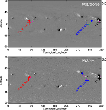
Figure 3. Magnetogram synoptic maps obtained from (a) the National Solar Observatory (NSO) Global Oscillation Network Group (GONG) (gong2.nso.edu/archive) and (b) SDO/HMI together with field lines computed via the PFSS model. The red, blue, and black crosses indicate the locations at 2.5 R⊙ of the IMF Parker spiral lines connecting to STEREO-A, STEREO-B, and L1, respectively. The green and purple traces mark the positive (outward) and negative (inward) open field lines computed via the PFSS model that connect the three spacecraft with the Sun. The red, blue, and black filled circles indicate the footpoints of these field lines on the photosphere. The locations of the footpoints of the field lines connecting with STEREO-A and L1 were similar using either GONG or HMI data, whereas the STEREO-B footpoints differ substantially.
Download figure:
Standard image High-resolution imageThis example illustrates how the configurations of the coronal magnetic field provided by the PFSS and MAS models can differ significantly, as discussed by Riley et al. (2006), who compared PFSS and magnetohydodynamic approaches. They found that whereas the PFSS and MHD solutions both capture the basic large-scale features of the corona, there can be notable discrepancies. Differences in the physics used in each model (PFSS assumes a current-free corona while MAS includes coronal plasma effects such as heating and energy transport processes) can lead to different configurations of closed and open field lines (note that for the simulations used here, the MAS model is run until a steady-state solution is found). Both PFSS and MAS are extremely sensitive to the choice of input magnetogram (e.g., Riley et al. 2011, 2012; Pahud et al. 2012). In particular, observatory-specific corrections to the line-of-sight magnetic field measurements can result in differences in the modeled coronal fields that may be more significant than those arising from the use of either the PFSS or the MAS model (Riley et al. 2006). Uncertainties in the input magnetogram due to the lack of polar and far-side observations and the use of old data near the east limb of the Sun (e.g., Nitta & DeRosa 2008; Schrijver & Title 2011) may also lead to ambiguous determination of the magnetic footpoint locations (e.g., Riley et al. 2006).
One way to decide which location for the STEREO-B footpoint is more likely to be correct is to check whether the polarity of the magnetic field observed in situ by this spacecraft at the time of the SEP event is consistent with the polarity of the connected field line inferred from the magnetograms (as shown for example in Figure 3). Figure 4 shows in situ observations from (left to right) STEREO-B, ACE, and STEREO-A. From top to bottom, we show (a) one-minute averages of electron intensities in two similar energy ranges measured by SEPT on STEREO and by EPAM on ACE, (b) the magnetic field magnitude as measured by the magnetometer on board STEREO (Acuña et al. 2008) and the magnetic field experiment on board ACE (Smith et al. 1998), (c) the elevation angle of the magnetic field vector in the RTN coordinate system, and (d) the azimuth angle of the magnetic field vector in the RTN coordinate system. For a spacecraft at ∼1 au and a solar wind speed of 400 km s−1, ∼315° corresponds to outwardly directed Parker spiral magnetic field, and ∼135° to an inward magnetic field. These directions are indicated by the dashed horizontal lines labeled OUT and IN, (e) the solar wind speed, (f) solar wind proton density, and (g) solar wind proton temperature as measured by the PLASTIC instruments on board the STEREO spacecraft (Galvin et al. 2008) and the SWICS instrument on board ACE (Gloeckler et al. 1998).
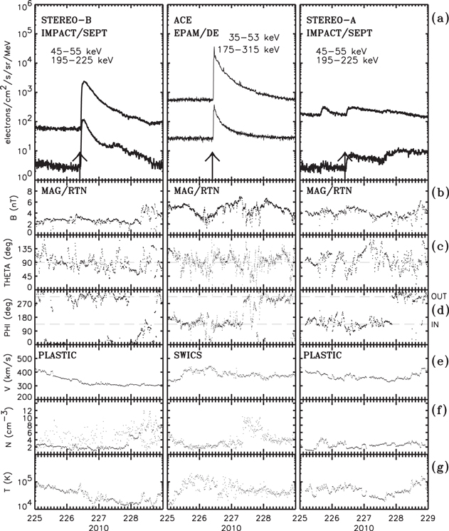
Figure 4. In situ observations as observed, from left to right, by STEREO-B, ACE, and STEREO-A. From top to bottom, (a) electron intensities, (b) magnetic field magnitude, (c)–(d) magnetic field polar and azimuthal angles in the RTN coordinate system, (e) solar wind speed, (f) solar wind proton density, and (g) solar wind proton temperature. The vertical black arrows in panels (a) identify the onset of the C4.4 soft X-ray flare at 09:38 UT.
Download figure:
Standard image High-resolution imageThe in situ observations show that at the onset of the SEP event, all three spacecraft were immersed in slow (≲450 km s−1) solar wind with inward magnetic field polarity in the case of ACE and STEREO-A but outward polarity in the case of STEREO-B. This polarity had persisted at STEREO-B since early on day 223. The coronal magnetic field models shown in Figure 3 indicate that both STEREO-A and ACE were connected to negative (inward) coronal fields, and this is consistent with the in situ magnetic field observations. However, only the PFSS and the WSA-ENLIL models applied to NSO/GONG magnetogram data correctly specify that STEREO-B was connected to positive (outward) coronal fields (see Figure 3(a) and Figure 2 of Park et al. 2015). The observation of an intense SEP event at STEREO-B with a relatively fast rise (left panel of Figure 4(a)) seems to favor a magnetic connection of this spacecraft to a region that is close to the site where the parent solar eruption took place, which is only provided by the PFSS model applied to NSO/GONG data (Figure 3(a)).
4. Solar Observations
4.1. Solar Flare
Figure 5 shows, from top to bottom, (a) soft X-ray intensities measured by GOES-14 and the intensities of the radio emissions as measured by (b) the Nançay Decametric Array (NDA), (c) the S/WAVES detector (Bougeret et al. 2008) on STEREO-B, (d) the WAVES experiment (Bougeret et al. 1995) on Wind, and (d) the S/WAVES detector on STEREO-A. The 1–8 Å light curve (Figure 5(a)) shows a modest C4.4 X-ray flare beginning at about 09:38 UT, peaking at 10:05 UT and ending at 10:31 UT. Although not illustrated here, 3–230 keV X-ray observations from the Ramaty High Energy Solar Spectroscopic Imager (Lin et al. 2002) show only a modest increase above the background at energies greater than 25 keV, indicating only moderate particle acceleration in the flare, at least for downward-directed electrons precipitating in the chromosphere.
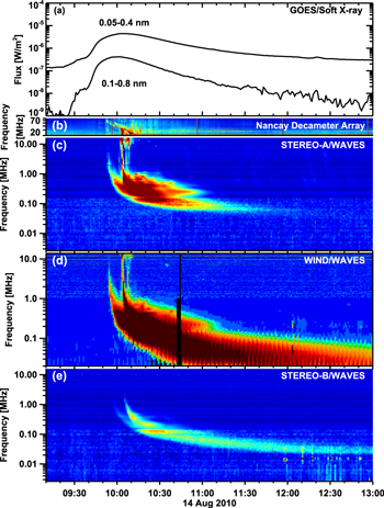
Figure 5. (a) One-minute averages of the 0.1–0.8 nm and 0.05–0.4 nm soft X-ray intensities measured by GOES-14. Radio measurements from (b) the Nançay Decametric Array in the frequency range 20–70 MHz, (c) the S/WAVES detector on STEREO-B in the frequency range 2.6 kHz–16 MHz, (d) the WAVES experiment on Wind in the frequency range 20 kHz–14 MHz, and (e) the S/WAVES detector on STEREO-A in the frequency range 2.6 kHz–16 MHz.
Download figure:
Standard image High-resolution imageFigure 5(b) shows a clear metric type II radio burst at frequencies ranging from ∼50 to 20 MHz starting at ∼09:52 UT and lasting until 10:12 UT (Bain et al. 2014). From fits to the type II burst emission, using the Newkirk (1961) and Baumbach-Allen radial density models, we find the burst was associated with a shock at heights between ∼1.25 and ∼1.95 R⊙, traveling at a speed of around 190–296 km s−1. Any extension of this type II radio burst from metric (Figure 5(b)) to decametric (DH) frequencies (Figures 5(c)–(e)) is not clearly observed. There are several possible reasons for this: there is a small frequency gap between the ground-based (NDA) and space-based radio observations (Wind and STEREO), so it is possible that the type II emission happened to cease within this frequency gap. Alternatively, the effective areas of the radio receivers and the levels of the galactic background noise between the instruments are different. Lecacheux (2000) estimated that the Nançay radio instrument is a factor of 100 more sensitive than the Wind instrument. In addition, Wind lost part of an antenna on 2000 August 3, which affected the sensitivity of the instrument (Meyer-Vernet 2001). Therefore, it is possible that any DH type II emissions present could have fallen below the detection limit of the Wind and STEREO radio receivers. Detailed inspection of the Wind (Figure 5(d)) and STEREO-A (Figure 5(c)) dynamic spectra reveals just a few short-duration "blobs" at frequencies above 7 MHz around 10:15–10:35 UT that perhaps were type II emissions but are not reported on the WAVES type II burst list at solar-radio.gsfc.nasa.gov/wind/data_products.html or cdaw.gsfc.nasa.gov/CME_list/radio/waves_type2.html. In fact, the SEP event on 2010 August 14 was one of the few events intense enough to be considered as a "Solar Proton Event affecting the Earth environment" by the Space Weather Prediction Center (SWPC) of the National Oceanic and Atmospheric Administration (ftp.swpc.noaa.gov/pub/inidces/SPE.txt), and which was associated with a fairly fast CME but lacked the clear DH type II emissions that usually accompany such events (e.g., Winter & Ledbetter 2015). Note that the >10 MeV proton peak intensity detected by GOES during the 2010 August 14 event was only 14 p.f.u, barely above the threshold of 10 p.f.u. required to be included in the SWPC event list.
A number of type III radio bursts were observed in association with this event. The onset of the first type III radio burst was recorded at about 09:51 UT by ground-based observatories (Bain et al. 2014). This type III radio burst can be tracked from metric to local plasma frequencies as observed by Wind/WAVES, indicating that the electron beams responsible for this emission were able to reach L1, with an intense local radio emission generated over a rather wide range of density fluctuations in the near vicinity of the spacecraft. High-frequency emissions from this type III burst were absent in the STEREO-B dynamic spectrum because the parent event occurred behind the limb (at W126°) from this spacecraft point of view and radiation was obscured by the intervening high-density plasma sphere through which the radiation was unable to propagate. STEREO-A did not observe low-frequency emissions of this type because of the directivity of the type III emission produced by the electron beams propagating mostly toward the east from the flare site along the Parker IMF lines as expected (cf. Figure 1(a)). A detailed study of this type III radio burst can be found in Reiner & MacDowall (2015).
A second intense type III burst at 10:03 UT appeared to emanate from the metric type II burst observed by NDA (starting at frequencies ≲35 MHz). A third type III burst at about ∼10:06 UT also seemed to emanate from the metric type II burst. These two type III bursts were more intense than the first type III burst at 09:51 UT and can be continuously tracked to DH frequencies in the Wind and STEREO-A dynamic spectra, but were only seen by STEREO-B at frequencies below ∼2 MHz because of occultation. The durations of these type III radio bursts at low frequencies were much longer in the Wind and STEREO-B observations than at STEREO-A (where the emissions ended at about ∼12:00 UT), most likely because of the directivity of the type III emission produced by the electrons propagating mostly along the Parker spiral IMF lines away from the STEREO-A location.
Type III radio bursts overlying type II bursts were originally termed shock-associated or shock-accelerated (SA) events, suggesting that the electron beams producing this radio emission were associated with the shock that generated the metric type II emission (Cane et al. 1981). This interpretation was later rejected because some events are observed with no underlying type II burst and it is now considered that the responsible electrons are accelerated in magnetic field reconnection processes occurring after the eruption of the CME (Cane et al. 2002). Since these late type III bursts occur after flare impulsive phases, they were named type III-l. There is a close association between type III-l and SEP events, indicating that particles accelerated in the aftermath of a CME can escape into the IP medium, and hence that such particles can contribute to large SEP events (Cane et al. 2002, 2010).
The event on 2010 August 14 also showed a type IV solar radio burst (at frequencies 150–442 MHz), moving at speeds 250–500 km s−1, that was cospatial with the core of the white-light CME (see details in Tun & Vourlidas 2013 and Bain et al. 2014). This moving type IV radio burst was consistent with gyrosynchroton emission by ∼1–100 keV electrons confined in the magnetic structure of the CME core with magnetic fields of the order of 5–15 Gauss as the CME propagated at ∼1 R⊙ above the solar surface (Tun & Vourlidas 2013; Bain et al. 2014). The synchrotron energy loss timescales for these electrons, expected to be several hours, suggest that the electrons were accelerated during CME initiation or the early propagation phase, possibly simultaneously with those particles observed in the SEP event, which, however, had access to open magnetic fields.
4.2. EUV and White-light Observations
Prior to the occurrence of the C4.4 flare and the eruption associated with the SEP event, EUV observations from SDO/AIA showed that a sigmoidal filament southwest of the sunspot pair formed by AR 11093 and AR 11099 began rapid expansion at around ∼09:00 UT on 2010 August 14 (Tun & Vourlidas 2013). EUV images from the Extreme Ultraviolet Imager (EUVI; Wuelser et al. 2004) of the Sun Earth Connection Coronal and Heliospheric Investigation (SECCHI; Howard et al. 2008) on board STEREO-A showed increased activity in the form of a filament rotation, also starting at ∼09:00 UT, and an expansion starting at ∼09:22 UT. SDO/AIA data showed a detachment of the western portion of the filament at 09:43 UT, after which an ejected filament appeared to unravel, rotating ∼90° until the western footpoint became the leading edge of the filament that eventually constituted the CME (see Figure 1 in Tun & Vourlidas 2013).
An asymmetric coronal bright front (i.e., EUV wave) was observed in association with this filament eruption. It propagated mainly toward the southern hemisphere, with no clear signature in the northern part of the solar disk. The eastern flank of the front (as seen from Earth), which was propagating toward the locations of the PFSS/GONG STEREO-B magnetic footpoint was clearly visible. The western flank was, however, not very clear and was affected by other active regions. Long et al. (2011a) used SDO/AIA observations to determine the kinematics of this EUV wave, showing that it initially moved with a velocity ranging from 379 ± 12 km s−1 to 460 ± 28 km s−1 (depending on the passband of the observations) and quickly decelerated at a rate of −128 ± 28 m s−2 to −431 ± 86 m s−2. These velocities and decelerations were measured at a specific arc sector over the solar surface centered on the AR and covering the southern latitudes (see Figure 1 in Long et al. 2011a). The front propagation in the other sectors seems to have been slower. STEREO-A/EUVI also detected the EUV wave, although with a lower cadence, providing slightly lower initial velocities and weaker deceleration (∼340 km s−1 and −72 m s−2) over a similar arc sector. Long et al. (2011a) described how the morphology of the EUV wave front was influenced by the plasma through which it propagated.
Whether or not the EUV wave actually arrives at the footpoint of the field line that connects to a particular spacecraft has been suggested as a discriminator to determine whether SEPs will be detected at that spacecraft (e.g., Rouillard et al. 2012; Park et al. 2013; Miteva et al. 2014). In order to obtain the EUV wave arrival times at the footpoints of the field lines connecting to each spacecraft in the case of the 2010 August 14 event, Park et al. (2015) used full-Sun difference images created by combining STEREO/EUVI 195 Å and SDO/AIA 193 Å observations. These authors determined the trajectory of the wave along great circles from the source region to the field line footpoints and used linear (constant speed) extrapolation to estimate the wave arrival time at each footpoint location, regardless of whether the wave was actually observed to reach the footpoint (cf. Figure 3 in Park et al. 2015). They determined the locations of the footpoints to be at W9° (CL = 306°) for STEREO-B, W57° (CL = 354°) for Earth, and W142° (CL = 81°) for STEREO-A, consistent with our estimates in Table 1, and established that the EUV wave reached the footpoints of STEREO-B at 09:56 UT ± 5 minutes, L1 at 09:30 UT ± 5 minutes, and STEREO-A at 09:57 UT ± 10 minutes. However, the use of a constant speed extrapolation to estimate the arrival times at the footpoints is questionable since the speed of the wave may vary due to the influence of the medium through which it propagates. Furthermore, there was no clear observational signature of the EUV wave reaching the STEREO-A field line footpoint.
In addition to visual identification of the EUV wave, it is possible to track the motion of the wave by computing the time variation of the EUV intensity increase along arcs of different radii lying within a sector that extends from the source of the wave and encompasses the estimated field line footpoint location (e.g., Lario et al. 2014). The technique used is similar to that described by Long et al. (2011b), Muhr et al. (2011), and Prise et al. (2014). We calculate the intensity increase in the running-difference 193 Å images from SDO/AIA and 195 Å images from STEREO-A/EUVI over three arc sectors centered at the active region source of the wave and including the footpoints of STEREO-B and STEREO-A. In particular, we use the STEREO-B footpoint locations provided by both the PFSS and WSA-ENLIL methods applied to NSO/GONG data as well as the Parker spiral footpoint location. The top panel of Figure 6 shows EUV intensity curves based on 193 Å SDO/AIA running-difference images along a 22 5-wide arc sector (or wedge) containing both the STEREO-B PFSS/GONG and STEREO-B Parker spiral footpoint locations. The middle panel shows the corresponding curves along a 225-wide arc sector containing the STEREO-B WSA-ENLIL footpoint. The lower panel shows the corresponding curves for a 45°-wide sector containing the STEREO-A magnetic footpoints but using 195 Å STEREO-A/EUVI observations. The curves represent the average intensity per pixel, assuming a 2° latitude resolution from the location of the parent active region. The units in the vertical axis of the three panels indicate the factor by which the intensity increased in the selected wedge.

Figure 6. EUV intensity increase at different times over three sector wedges covering the distance from the parent active region to the footpoint of STEREO-B identified using either the PFSS/GONG or the Parker projection method (top panel), STEREO-B using the WSA-ENLIL method (middle panel), and STEREO-A (bottom panel) using the PFSS and Parker projection model. The vertical dotted lines indicate the location of footpoints along the sector wedge (note that the STEREO-A PFSS and Parker models provide foopoint locations that only differ by a few degrees so only one vertical line is shown). For clarity purposes, curves after time 10:18:08 UT in the middle panel have been shifted vertically by a value of 1. The EUV intensity in the sector wedges including the STEREO-B footpoints shows a clear peak moving toward the footpoints that is able to reach the STEREO-B footpoints using either PFSS/GONG or Parker spiral projection but not the WSA-ENLIL footpoint. In the sector wedge including STEREO-A footpoints, there is no clear moving peak.
Download figure:
Standard image High-resolution imageThe top panel of Figure 6 shows a clear moving intensity peak associated with the brightest part of the EUV front that arrived at the STEREO-B PFSS/GONG footpoint well before ∼09:51 UT and at the Parker spiral footpoint at around ∼10:03 UT. The middle panel of Figure 6 shows that the EUV wave front propagated along this arc sector with clear signatures up to ∼10:15 UT, but after this time, the EUV wave front signatures were not so apparent, and its arrival at the STEREO-B WSA-ENLIL footpoint was not clearly observed. Similarly, the lower panel of Figure 6 shows that no moving wave signature was present near the STEREO-A footpoint location. There may be some weak signatures of intensity disturbances closer to the site of the parent active region, but these do not show a clear propagation pattern. Although not shown in Figure 6, a similar analysis indicates that the EUV wave reached the footpoints of field lines connected to Earth shortly after the eruption at ≲09:30 UT.
As the EUV waves propagate outward, they are usually followed by expanding dimmings, which are cospatial with the white-light cavity of the CMEs (e.g., Thompson et al. 2000; Zhukov 2011). Figure 7 shows the changes in a sequence of 193 Å SDO/AIA images with respect to the similar image taken at 08:00:07 UT on 2010 August 14. The sequence of images clearly shows the evolution of the dimming (dark region) expanding south of the parent active region. Dimmings are signatures of material being evacuated from the corona as magnetic field opens in the wake of the CME (e.g., Sterling & Hudson 1997). EUV dimmings are an indication of the location and extent of the white-light CME, but not of the shock formed in front of it, which may extend to a broader region than that indicated by the dimming. White-light images taken by the SOHO/LASCO C2 coronagraph can be seen in Figure 8. The CME was clearly deflected southward with respect to the radial direction above the parent active region. Liewer et al. (2015) imputed the southward deflection to the magnetic field pressure created by active regions adjacent to the site where the eruption took place. They also indicated that the magnetic field pressure would produce a more modest eastward deflection. We refer the reader to Liewer et al. (2015) for details on the WL observations of the CME.
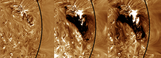
Figure 7. Changes of the 193 Å intensity in SDO/AIA images taken at (from left to right) 09:20:07, 10:00:07, and 10:40:07 UT on 2010 August 14 with respect to the 193 Å SDO/AIA image taken at 08:00:07 UT on 2010 August 14. The dark area is an indication of evacuated material at the south of the parent active region (bright).
Download figure:
Standard image High-resolution image
Figure 8. Sequence of white-light images taken by the SOHO/LASCO C2 coronagraph at, from left to right, 10:12:05, 10:24:05, 10:48:05, and 11:00:06 UT on 2010 August 14. The CME deflected southward with respect to the radial direction above the parent active region at N13°.
Download figure:
Standard image High-resolution image4.3. CME Front Shock
Under the assumption that SEPs are accelerated by shocks that form low in the corona (e.g., Cliver et al. 1995 and references therein), and that the accelerated particles then stream out into IP space along open field lines connected to the shock, it is essential to identify the extent of these shocks and when, if at all, they intercept field lines connecting to the observing spacecraft. Signatures of CME-driven shocks in WL coronagraph observations were investigated by Ontiveros & Vourlidas (2009). They concluded that the shocks initially driven by CMEs can be identified with sharp but faint brightness enhancements seen ahead of and around bright CME fronts in coronagraph images (see, e.g., their Figure 1).
In the STEREO era, techniques of shock identification have been enhanced by combining EUV and WL observations from multiple viewpoints. In particular, here we will use the compound geometric model developed by Kwon et al. (2014) to determine the three-dimensional (3D) structure of the CME associated with the 2010 August 14 SEP event using EUV and WL data from STEREO-A, STEREO-B, SDO, and SOHO. An ellipsoid shape centered at a certain altitude hE is used to describe the outermost front driven by the CME. Components of the CME, such as the bright frontal loop or three-part CME structure, which may include a flux rope-like structure, are described by the Graduated Cylindrical Shell (GCS) model (Thernisien et al. 2009; Thernisien 2011). The fitting is done via a forward-modeling approach. Selected sequential images of the event from three viewpoints are produced by combining EUV data from STEREO/SECCHI/EUVI and SDO/AIA, as well as WL data from the coronagraphs COR-1 and COR-2 of STEREO/SECCHI (Howard et al. 2008), and the SOHO/LASCO C2 and C3 coronagraphs. The images should be as cotemporal as possible to minimize evolutionary effects on the event morphology. The assumed geometric shapes—GCS for the magnetic-flux-rope-like structure, and the ellipsoid for the shock front—are projected onto the three spacecraft images, taking into account the viewing prespective and then manipulated until a visually satisfying fit is obtained for all viewpoints simultaneously. In this respect, the fits are approximations to the actual shape of the shock front and flux rope. The GCS model has seven free parameters: the height, longitude, and latitude of the center of the flux rope, as well as the half angle, aspect ratio, height, and rotation of the flux rope, as described in detail by Thernisien (2011). The ellipsoid model also uses seven free parameters: the height, longitude, and latitude of the center of the ellipsoid; the length of the three semi-principal axes; and rotation angle of the ellipsoid (see details in Kwon et al. 2014).
The first three columns of Figure 9 show, for different times (running vertically), representations of the outermost front using the ellipsoid model overplotted on a combination of running-difference images from SDO/AIA and SOHO/LASCO (center column), and STEREO-B (left) and STEREO-A (right) SECCHI EUVI, COR-1, and COR-2. (For clarity, the modeled GCS flux rope is not represented.) To help visualize the 3D shape of the front, each quadrant of the front is shown by a different color line (red, orange, blue, and cyan). The green circle identifies the maximum extension of the outermost shock front. Dashed lines are used when the reconstructed geometric shape lies behind the plane of the figure. Blue, black, and red dots in the first three top panels of Figure 9 indicate the PFSS/GONG locations of the STEREO-B, L1/Earth, and STEREO-A field line footpoints.

Figure 9. First three columns: selected time series observations of the CME in composite images taken by STEREO-B, SDO and SOHO, and STEREO-A (from left to right). The solar center is located at the center of each panel and the solar rotational axis is directed toward the top of each image. The white circle in each panel indicates the solar disk. Images at the center of each panel are running-difference images from STEREO/SECCHI/EUVI 195 Å in the first and third columns and running ratio images from SDO/AIA 193 Å in the second column. White-light observations are running-difference images from STEREO/SECCHI/COR-1 and STEREO/SECCHI/COR-2 in the first and third columns and SOHO/LASCO/C2 in the second column. Different quadrants of the reconstructed 3D shock front are indicated by the red, orange, blue and cyan lines. Dashed lines are used when the 3D structure is located below the plane of the image. Right column: projection of the ellipsoid shock front in the ecliptic plane as seen from the north ecliptic pole. Gray lines indicate the 3D structure of the ellipsoid. The red, blue, and black lines indicate the magnetic field lines connecting to STEREO-A, STEREO-B, and L1, respectively, computed assuming Parker IMF lines above 2.5 R⊙ and the PFSS/GONG configuration below 2.5 R⊙ (gray is used for the portion of the field line inside the modeled ellipsoid). The red, blue, and black arrows indicate the radial directions to STEREO-A, STEREO-B, and L1, respectively.
Download figure:
Standard image High-resolution imageAs seen in Figure 9, the eruption initiating the CME and shock was located to the south of AR 11093 (at N13°W54°, close to the L1 footpoint (black dot) in the first SDO image). The series of ellipsoid model fits indicates that the directional axis of the shock front moved southward from N04°W50° (CL = 347°) at ∼09:55 UT to S24°W52° by ∼10:54 UT when the leading edge of the shock was at ∼8 R⊙. The axis latitude of S24° was then maintained as the shock propagated to distances of ∼15 R⊙ and at least until 12:24 UT. Consistent with this southward motion, Liewer et al. (2015) applied the GCS model to determine that the CME flux rope was directed toward S13° and CL = 341°, giving a southward (eastward) deviation relative to the parent active region of 25° (11°).
The right column of Figure 9 shows the projection of the ellipsoid shock front onto the ecliptic plane as seen from the north ecliptic pole. The black circle in the center of each figure indicates a distance of 1 R⊙; note that the scale changes between the top and lower panels. The arrows in Figure 9(d) indicate the direction to each spacecraft projected onto the ecliptic plane. IMF lines connecting STEREO-B (blue), STEREO-A (red), and near-Earth spacecraft (black) with the Sun are also shown. These are estimated using Parker spiral field lines from the spacecraft down to a heliocentric distance of 2.5 R⊙ and PFSS/GONG model field lines below this distance; the clear kink in the STEREO-A field line in Figure 9(d) occurs at this height. Since the field direction is likely to change with passage of the shock, field lines that remain inside the fitted ellipsoid are shown in gray. Furthermore, as the solar eruption occurs and the shock starts expanding, the field configuration assumed in the model may be destabilized. Therefore, the field configuration shown in Figure 9(d) is only an approximation of the magnetic fields that the traveling shock will encounter as it expands away from the Sun.
Because of the close proximity between the site of the parent solar eruption and the footpoint of the magnetic field line connecting Earth with the Sun, the shock front established contact with the field line connected to L1 nearly simultaneously with the parent solar eruption. Figure 9(d) shows that, at the time of the observations in the top row of the figure (∼09:55 UT), near-Earth observers were magnetically connected with the shock near its nose. STEREO-B was also already connected with the shock at this time but near its eastern flank (as seen from Earth). However, STEREO-A had not yet established magnetic connection with the fitted shock. Connection had evidently already taken place by the time of Figure 9(h) (∼10:54 UT), and intermediate fits to the shock, not shown here, indicate that STEREO-A connection to the western flank of the shock (as seen from Earth) occurred at ∼10:30 UT.
The time evolution of the fitted ellipsoid allows the shock propagation speed to be estimated at the point where the field line connecting to a particular spacecraft intersects the shock front; this point is named the "cobpoint" (Connecting with the OBserver point), after Heras et al. (1995). Figure 10 shows the speed of the shock (black symbols) at the cobpoints for (a) STEREO-B, (b) near-Earth observers, and (c) STEREO-A as a function of time (top panels) and as a function of the cobpoint radial distance above the solar surface (bottom panels). We use the field lines provided by the PFSS/GONG method. The first point in each plot corresponds to either the first time that the geometrical shape assumed in the model by Kwon et al. (2014) could be fitted to the EUV and WL images (i.e., 09:50 UT) or the time when the connection between the fitted shock and the field line connecting to each spacecraft is established.
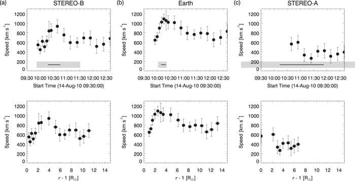
Figure 10. Speed of the ellipsoid shock front at the point on the shock that is magnetically connected to (a) STEREO-B, (b) near-Earth observers, and (c) STEREO-A as a function of time (top row) and radial distance from the solar surface (bottom row). The horizontal thin black lines in the top panels indicate the estimated proton release times, whereas the horizontal gray bars indicate the errors in these estimated release times as described in Section 5.
Download figure:
Standard image High-resolution imageThe shock speed at the Earth cobpoint rapidly increased to ≲1200 km s−1 at ∼10:12 UT, and though then decelerating, it maintained speeds above 600 km s−1 for at least the next two hours. The acceleration was more gradual at the STEREO-B cobpoint, reaching ≲1000 km s−1 at ∼10:40 UT, then declining to speeds around 600 km s−1. As noted above, the STEREO-A connection to the shock was delayed. The shock speed at the STEREO-A cobpoint when connection occurred was lower (∼600 km s−1) than the speeds attained at the other spacecraft cobpoints, and rapidly declined to around 400 km s−1. The bottom panels of Figure 10 indicate that Earth was connected with the shock even before the time when we can reconstruct the initial 3D structure of the shock using the method of Kwon et al. (2014). At this time, Earth's cobpoint was already located on the central part of the fitted shock at ∼1 R⊙ above the solar surface (heliocentric distance r ∼ 2 R⊙), with shock speeds above 600 km s−1. On the other hand, both STEREO-B and STEREO-A established initial connection with the flanks of the fitted shock when their cobpoints were close to the solar surface. Whereas the highest speed of the shock at the Earth cobpoint was reached at 2.5 R⊙ above the solar surface at ∼10:12 UT, the highest speed at the STEREO-B cobpoint was reached later (∼10:40 UT) at ∼3.9 R⊙. By contrast, the shock speeds at the STEREO-A cobpoint decreased substantially with distance to values ≲400 km s−1.
This event has also been studied independently by co-author Xie and colleagues using a similar forward-modeling technique, employing the GCS model to fit the magnetic-flux-rope-like structure and an oblate spheroid shock model to fit the CME shock (Xie et al., "Comparison on the CME-shock Acceleration of Three Widespread SEPs during Solar Cycle 24," manuscript under preparation, 2017). They conclude that the shock front intercepted Parker spiral field lines connecting to Earth, STEREO-B, and STEREO-A at ∼09:52 UT, ∼10:00 UT, and ∼10:40 UT, respectively. The heliocentric distances of the cobpoint at these times were 2.0 R⊙, 1.8 R⊙, and 1.3 R⊙, respectively. These connection times and cobpoint distances are reasonably consistent with those obtained above other than the times being a few (≲10) minutes later. The propagation direction of the major axis of the CME shock (flux rope) was N03°W50° (S01°W50°) at 10:00 UT, S10°W50° (S10°W50°) at 10:40 UT and S25°W40° (S15°W45°) at 11:45 UT, indicating that the structure expanded asymmetrically with a clear southward bias, as also concluded above.
Although the GCS+shock models discussed above provide a good match to the shape of this CME in its early stages, the bright front became more complex and difficult to fit later, especially in the northern portion where the CME may have interacted with a pre-existing streamer (within the time resolution of the images, interaction between the northern coronal streamer and the fitted shock occurred at a time ≲09:55 UT), and also in the southernmost portion of the shock (see Figures 9(i)–(k)) due to the asymmetric CME expansion (Liewer et al. 2015). Therefore, we should keep in mind that the idealized geometric shapes used to describe the large-scale structure of the shocks are approximations to the actual shape of the shocks.
Above we discussed the metric type II burst that was observed between 09:52 UT and 10:12 UT, and inferred that the burst was associated with a shock at heights of ∼1.25–1.95 R⊙ and traveling at around 190–296 km s−1. However, at this time, the leading edge of the shock fitted to EUV and WL observations by both methods was already at heliocentric distances >2 R⊙ (e.g., 2.05 R⊙ at 09:55 UT and 3.15 R⊙ at 10:10 UT when using the model by Kwon et al. 2014) and moving at a faster speed. Therefore, if the shock responsible for the metric type II emission was the same shock observed in EUV and WL, the metric type II radio emission must have been generated from those portions of the shock propagating low in the solar corona, moving more slowly than the leading edge of the shock, and most likely interacting with denser regions of the corona (see similar examples in, e.g., Feng et al. 2013 and references therein).
5. SEP Observations
5.1. Particle Release Times
One method to determine when a spacecraft in IP space establishes magnetic connection with an SEP source is to estimate the time when the SEPs detected by this spacecraft were released onto the IMF line connecting to such spacecraft. Inferring the release time of SEPs from in situ observations at 1 au is not a straightforward task. There are many unknown variables involved in the arrival of particles at the spacecraft. These include the actual length and shape of the IMF line along which particles propagate, the particle transport conditions in the low corona and IP space, and the processes of particle acceleration and release that may depend on particle energy and species. In addition, there may be difficulties in determining the exact time of the SEP event onset. A low instrument sensitivity, or a low signal-to-noise ratio (high background) at the beginning of the event may lead to an apparent delay in the observed onset. Low counting statistics and uncertainties in the instrument response may also introduce errors in the onset time.
In order to define the onset of the SEP event at a certain energy, several criteria have been commonly used. One is to define the onset as the time when the particle intensity rises above the pre-event average background by a certain factor expressed in units of the statistical error of the pre-event counting rate (e.g., Papaioannou et al. 2014) or more qualitatively, by visual inspection of suitably scaled intensity–time plots. Another procedure is to use the cumulative sum (CUSUM) method to calculate the normalized time-integrated excess of the counting rate above the background or pre-event intensity level (Torsti et al. 1998). Huttunen-Heikinmaa et al. (2005) modified this method for the case when data follow a Poisson distribution (known as the Poisson-CUSUM method). Another method, known as the "Fixed-Onset-Level" method, defines the onset as an increase of the particle intensity above a fixed fraction of the maximum intensity of the event (Xie et al. 2016). Still another method consists of making linear fits to both the background intensity and the increasing logarithmic intensity and then taking the intersection of the two fitted lines as the onset time, similar to the intersection slope method used by Miteva et al. (2014). An alternative method proposed by Masson et al. (2012) uses well-defined reference times during the rising phase of the intensity–time profiles at different energies to define an energy-dependent rise time that can then be used to determine an upper limit of the particle release time and thus avoiding the fluctuations of the pre-event intensities.
When the onset of the SEP event has an abrupt, prompt increase, all techniques usually provide similar results. However, this may not be the case for events with slow rising onsets, where the onset time is ill-defined, or for weak events with low counting statistics. The statistics can be improved by using longer time averages at the expense of losing time resolution or, at the expense of losing energy resolution, by summing count rates in consecutive energy channels. Here we compare the onset times obtained when applying either the Poisson-CUSUM method, the Fixed-Onset-Level method, or an alternative method identifying the onset of the SEP event by eye.
Figure 11 shows in detail the onset of the 2010 August 14 SEP event as observed by the proton channels of (a) the Low-Energy Detector (LED) and High-Energy Detector (HED) of the SOHO/ERNE instrument; (b) the Low-Energy Telescope (LET; Mewaldt et al. 2008) and HET of STEREO-B; and (c) the LET and HET on board STEREO-A. The small black dots are one-minute resolution proton intensities and the red lines are longer-term averages (5 minutes for SOHO/ERNE/LED, 3 minutes for SOHO/ERNE/HED, 4 minutes for STEREO-B/LET, 15 minutes for STEREO-B/HET, 10 minutes for STEREO-A/LET, and 1 hr for STEREO-A/HET). Note that the STEREO/HET data have been combined into three broad energy channels to improve the particle statistics.
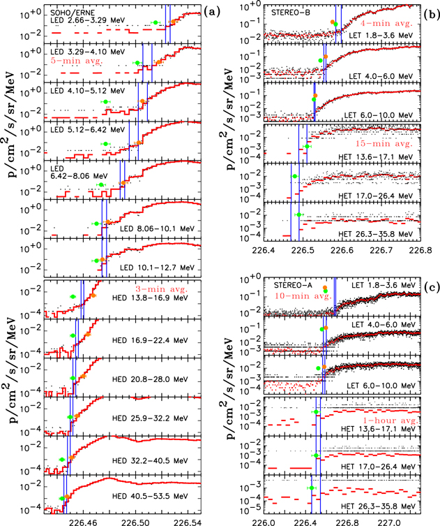
Figure 11. Onset of the 2010 August 14 SEP event as observed in selected proton energy channels of (a) SOHO/ERNE/LED (top) and SOHO/ERNE/HED (bottom), (b) LET (top) and HET (bottom) on board STEREO-B, and (c) LET (top) and HET (bottom) on board STEREO-A. The black dots are one-minute averages, whereas the red lines are long-term averages (as indicated in the figure). The blue vertical lines indicate the uncertainty in the onset of the event when identified "by eye," while the green and orange dots indicate the onset times obtained using the Poisson-CUSUM and Fixed-Onset-Level methods, respectively.
Download figure:
Standard image High-resolution imageThe blue solid vertical lines in each panel of Figure 11 indicate the time interval where the onset of the event has been identified "by eye" using the longer-term averages according to the following criteria: the second vertical blue line indicates the time after which the longer-term averaged intensities are statistically significant above the pre-event intensities (by a factor of ∼2σ) and do not return to the values registered before the first vertical line. The time interval between the two vertical lines indicates the uncertainty in the onset time determination. In cases where the particle increase is particularly rapid, this "by-eye" method may be also applied to higher resolution, e.g., one-minute-averaged, data.
The green dots in Figure 11 indicate the onset of the event identified by applying the Poisson-CUSUM method to the longer-term averaged data. The orange dots indicate onset times identified using the Fixed-Onset-Level method (see details in Xie et al. 2016) with one-minute resolution SOHO/ERNE and STEREO/LET proton intensities. Specifically, the onset time is defined as the time when the intensity is both at least 3σ deviations above the background level and reaches 1.0% of the maximum event intensity for SOHO/ERNE observations, 1.2% for STEREO-B/LET, and 5.5% for STEREO-A/LET. Since the background-to-peak level changes with varying SEP energies and intensity profiles, these fractions are dependent on spacecraft and are arbitrarily chosen to minimize the background effect on the determination of the SEP release times. Details and justifications can be found in Xie et al. (2016).
As is evident in Figure 11, there may be significant discrepancies in the determination of the onset times by the different methods. For example, single point increases in the five-minute-averaged intensities observed after day 226.46 in the 4.10 to 8.06 MeV energy channels of SOHO/ERNE/LED (Figure 11(a)) lead to early estimations of the onset times when using the Poisson-CUSUM method. The Fixed-Onset-Level method may produce different results depending on the value chosen for the percentage of the maximum event intensity required to define the event onset. Similarly, the identification of the onset times by eye involves subjectivity that may depend on how the data are presented and the opinion or bias of the person interpreting the data.
Having obtained the particle event onset times at the spacecraft, the next step is to estimate the particle release time at the Sun. Figure 12 shows the results of velocity dispersion analysis (VDA) applied to the event as observed by (a) STEREO-B, (b) near Earth, and (c) STEREO-A. The VDA method consists of plotting the onset times at different energies versus c/v = 1/β, where v is the particle speed and c is the speed of light. It assumes that (1) the SEP injection profile is energy independent and has an impulsive onset, and (2) the first-arriving particles observed at the spacecraft propagate scatter free, with pitch-angle cosines  along a common travel distance D from their coronal injection site to the observer. The green diamonds in the top row of Figure 12 indicate the proton onset times determined by eye, indicated by blue vertical lines in Figure 11, plotted against 1/β. Similarly, the Poisson-CUSUM proton onset times from Figure 11 are shown in middle row of Figure 12, and the Fixed-Onset-Level proton onset times are shown in the bottom row. Note that the Fixed-Onset-Level STEREO proton onset times only use LET observations. Electron onset times are also shown in the top and bottom rows of Figure 12, usually by red dots (as described in the figure caption). We note that these electron onset times may be in error if high-energy electrons scattered within each instrument contribute to the intensities measured in lower energy channels, producing an earlier than expected onset (e.g., Haggerty & Roelof 2003). Although no corrections have been applied to the electron onset times in Figure 12, and therefore they should be considered with caution, the high-energy electron intensities were not too elevated in this event, so contamination in the lower energy channels is not expected to be severe.
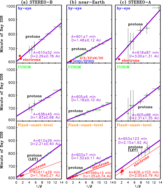
Figure 12. Velocity dispersion analysis (VDA) of the onset of the event at (a) STEREO-B, (b) L1, and (c) STEREO-A. The green symbols indicate the proton onset times identified in Figure 11 "by eye" (top panels), by the Poisson-CUSUM method (middle panels), and by the Fixed-Onset-Level method (bottom panels). The red symbols in the top panels indicate the electron onset times identified "by eye" using (a) the 225–255 keV electron intensities observed by the sunward-looking telescope of the STEREO-B/SEPT and the 0.7–1.4 MeV electron intensities from the STEREO-B/HET, (b) the 0.25–0.70 MeV electron intensities from the Electron Proton Helium Instrument (EPHIN; Müller-Mellin et al. 1995) on board SOHO (blue dot), and electron intensities measured in the sunward direction from the highest energy (175–315 keV) electron channel of ACE/EPAM/DE (red dot), and (c) the 195–225 keV electron intensities from the sunward-looking telescope of STEREO-A/SEPT; no significant relativistic electron increase was observed by the STEREO-A/HET. The red symbols in the bottom panels indicate the electron onsets times identified using the Fixed-Onset-Level method in several energy channels of (a) STEREO-B/SEPT, spanning 65–295 keV, (b) the Wind/3DP instrument (Lin et al. 1995), spanning 27–100 keV, and SOHO/EPHIN, spanning 250–700 keV, and (c) STEREO-A/SEPT, spanning 45–105 keV (onset levels were fixed at 1% of the peak intensity for L1 data, 2% for STEREO-B/SEPT, and 88% for STEREO-A/SEPT). The purple and red straight lines are linear regression fits to proton and electron data points, respectively. The legends give the estimated release time (A) and the path length (D) discussed in the text.
Download figure:
Standard image High-resolution imageThe purple straight lines in Figure 12 are least-squares fits to the proton onset times at different energies given by the expression ti = A + D/vi, where ti is the onset time in the energy channel detecting particles of speed vi. Here, vi is the speed of particles with an energy that is equal to the geometrical mean of the energy window of the channel, A is the release time of the particles at the Sun, and D is the distance traveled by these particles. Similarly, the red straight lines in the bottom row of Figure 12 are the least-squares fits to the electron onset times. The intercept of each least-squares fit line with the vertical axis gives an individual estimate of the particle release time, while the slope gives an estimate of the effective path length D followed by the particles to reach the spacecraft. Distances that exceed the length of the nominal Parker spiral IMF lines (given in column 7 of Table 1) may result, for example, from non-Parker-spiral IMF configurations, delays in the release of lower energy particles, a non-impulsive release of particles, and/or energy-dependent transport processes (e.g., Richardson et al. 1991; Kahler & Ragot 2006; Leske et al. 2012; Rouillard et al. 2012; Laitinen et al. 2015). The inferred path length for each fit is shown in Figure 12. They suggest a proton path length to Earth that slightly exceeds the nominal spiral field line length, a longer path length for STEREO-B of around 2 au, but with an uncertainty of around 0.7 au, and an even longer path length of 2–3 au, but with an uncertainty of around 1.5 au, for STEREO-A. For this event, the lack of IP transients observed immediately prior to the event suggests that IMF lines did not deviate significantly from Parker spiral field lines. This implies that an energy-dependent injection or transport may be possible explanations for path lengths longer than the nominal Parker lengths, and these would invalidate the use of the VDA method. On the other hand, although path lengths longer than the Parker spiral field line lengths are found here, there are also large uncertainties in these estimates, so it is unclear whether they actually suggest that the VDA method is invalid.
We have also estimated the release time at the Sun of particles in specific energy channels by assuming that they propagate scatter free along nominal Parker spiral IMF lines (i.e., "time-shift analysis," TSA). Although this removes the VDA assumption that particles of all energies are released simultaneously, it makes the possibly erroneous assumption that particle propagation is scatter free along nominal spiral field lines. Unlike VDA, where onset times from multiple energy channels are combined to give one SEP release time estimate, with TSA, each energy channel provides an independent estimate of the release time.
Column 2 of Table 2 summarizes the various estimates of the release times of SEPs observed by each spacecraft using either the VDA or TSA method applied to electrons and protons. These use the onset times identified with the different methods discussed in relation to Figure 11. Note that the ∼8 minute light travel time from Sun to 1 au has been added to the release times so that they may be directly compared with the detection times of solar electromagnetic emissions, such as those discussed above.
Table 2. Particle Release Times and Cobpoint Height and θBn at these Times
| Particle Species/Spacecraft/Instrument | Estimated | Cobpoint Height | θBn |
|---|---|---|---|
| Release | above Sun | at the | |
| Time [UT]a | Surfaceb | Cobpointc | |
| (1) | (2) | (3) | (4) |
| Protons/SOHO/ERNE (2.66–67.3 MeV) | 10:09 ± 7 minutes (eye, VDA) | 2.0 ± 0.7 R⊙ | 190 ± 97 |
| Protons/SOHO/ERNE (2.66–67.3 MeV) | 10:13 ± 6 minutes (CU, VDA) | 2.4 ± 0.6 R⊙ | 121 ± 19 |
| Protons/SOHO/ERNE (2.66–67.3 MeV) | 10:11 ± 7 minutes (FL, VDA) | 2.2 ± 0.7 R⊙ | 116 ± 23 |
| 51–67 MeV Protons/SOHO/ERNE | 10:20 ± 2 minutes (eye, TSA) | 3.1 ± 0.3 R⊙ | 138 ± 17 |
| 175–315 keV Electrons/ACE/EPAM/DE | 10:11 ± 2 minutes (eye, TSA) | 2.2 ± 0.2 R⊙ | 120 ± 13 |
| 0.25–0.70 MeV Electrons/SOHO/EPHIN | 10:08 ± 2 minutes (eye, TSA) | 1.9 ± 0.2 R⊙ | 112 ± 13 |
| Electrons/Wind/3DP and SOHO/EPHIN (25–700 keV) | 10:07 ± 3 minutes (FL, VDA) | 1.8 ± 0.3 R⊙ | 109 ± 16 |
| Protons/STEREO-B/LET-HET (1.8–36 MeV) | 10:18 ± 19 minutes (eye, VDA) | 2.2 ± 1.7 R⊙ | 424 ± 110 |
| Protons/STEREO-B/LET-HET (1.8–36 MeV) | 10:46 ± 45 minutes (CU, VDA) | 4.1 ± 3.5 R⊙ | 398 ± 136 |
| Protons/STEREO-B/LET (4–12 MeV) | 10:21 ± 29 minutes (FL, VDA) | 2.6 ± 2.5 R⊙ | 449 ± 174 |
| 17–26 MeV Protons/STEREO-B/HET | 10:46 ± 15 minutes (eye, TSA) | 4.4 ± 1.5 R⊙ | 334 ± 070 |
| 225–255 keV Electrons/STEREO-B/SEPT | 10:23 ± 10 minutes (eye, TSA) | 2.4 ± 1.2 R⊙ | 431 ± 102 |
| 0.7–1.4 MeV Electrons/STEREO-B/HET | 10:46 ± 5 minutes (eye, TSA) | 4.5 ± 0.7 R⊙ | 318 ± 043 |
| Electrons/STEREO-B/SEPT (65–295 keV) | 10:19 ± 29 minutes (FL, VDA) | 2.5 ± 2.4 R⊙ | 490 ± 210 |
| Protons/STEREO-A/LET-HET (1.8–36 MeV) | 10:26 ± 87 minutes (eye, VDA) | dToo early for shock connection | |
| Protons/STEREO-A/LET-HET (1.8–36 MeV) | 10:13 ± 88 minutes (CU, VDA) | dToo early for shock connection | |
| Protons/STEREO-A/LET (4–10 MeV) | 11:01 ± 123 minutes (FL, VDA) | d2.6 ± 0.5 R⊙ | 450 ± 39 |
| 17–25 MeV Protons/STEREO-A/HET | 11:53 ± 60 minutes (eye, TSA) | d4.8 ± 0.7 R⊙ | 415 ± 32 |
| 195–225 keV Electrons/STEREO-A/SEPT | 10:21 ± 10 minutes (eye, TSA) | Too early for shock connection | |
| Electrons/STEREO-B/SEPT(45–105 keV) | 10:34 ± 103 minutes (FL, VDA) | d0.0 ± 0.0 R⊙ | 178 ± 05 |
Notes.
aLight travel time already added. The method used to identify the onset times is indicated by "eye" when using the vertical blue lines in Figure 11, "CU" for the Poisson-CUSUM method, and "FL" for the Fixed-Onset-Level method. The method used to estimate the particle release time is indicated by "VDA" for velocity dispersion analysis and "TSA" for time-shift analysis using the nominal Parker spiral length. bShock height estimated at the cobpoint of each spacecraft using the using the fitted ellipsoid shock and PFSS/GONG model field lines. The range of heights includes the uncertainty in the estimated SEP release time. cAngle between the normal to the ellipsoid shock front and the magnetic field direction at the cobpoint (estimated using the PFSS/GONG method). dErrors in the particle release times for STEREO-A are neglected since the shock front has already left the field of views of the coronagraphs during the time ranges given by the release time errors. Thus, only errors in the 3D geometry of the shock are considered.Download table as: ASCIITypeset image
Considering first the estimated release times of the particles detected at Earth, because of rapid increase in intensity, the observed electron onset times in individual channels can often be estimated to within 2–3 minutes. This is reflected in the small errors in both the TSA- and VDA-estimated release times, which cover a range from 10:07 UT ± 3 minutes to 10:11 UT ± 2 minutes. The proton release times are also characterized to a few minutes, and range from 10:09 UT ± 7 minutes to 10:20 UT ± 2 minutes, possibly suggesting a slight delay relative to electrons, but also consistent, within errors, with a simultaneous release. The thin horizontal black line in the top panel of Figure 10(b) indicates the time interval when proton release occurred as estimated by the different methods listed in Table 2, whereas the gray horizontal bar includes the estimated errors.
For STEREO-B, the estimated release times range from 10:19 UT ± 29 minutes to 10:46 UT ± 5 minutes for electrons, and 10:18–10:46 UT for protons, with more generous uncertainties. These results suggest a delay in the particle release time at STEREO-B compared with that for the particles detected at Earth, but zero delay is also not ruled out by the uncertainties. Because of the slower event onset at STEREO-A, the release times are even more uncertain, but suggestive of a longer delay than at STEREO-B. The electron release times range over 10:21 UT (TSA) to 10:34 UT (VDA, but with a large uncertainty), while proton release times are from 10:13 to 11:53 UT, again with large uncertainties. Thus, whereas the different methods provide similar release times for L1 observations, the uncertainties and range of release times increase for STEREO-B and STEREO-A. The variability of release times obtained by the different methods applied to STEREO-A data clearly indicates that these methods should be judiciously considered in the case of weak gradual particle intensity increases.
5.2. Height of the Shock at SEP Release Time
Having obtained the estimated release times of the SEPs detected at each spacecraft, we can evaluate the heights of the cobpoint at that time using the modeled 3D geometry of the shock, as discussed in Section 4.3 and previously shown for other events in Lario et al. (2014, 2016). In particular, column 3 of Table 2 lists the height above the solar surface of the cobpoint of each spacecraft at the respective release time assuming PFSS/GONG magnetic field lines and an ellipsoid-shaped shock as shown in Figure 9. The error in the cobpoint height listed in Table 2 corresponds to the change in this height during the time interval that contains the uncertainty in the SEP release time. Note that cobpoint heights for STEREO-A are just given for the estimated particle release times without considering the errors since including these errors encompasses times that are prior to the parent solar eruption and after the shock front has left the fields of view of the coronagraph images, when the ellipsoid fitting is not possible. We can also estimate the angle θBn between the magnetic field upstream of the shock and the normal to the fitted shock, both evaluated at the cobpoint of each spacecraft, as listed in column 4 of Table 2 (similar estimates for other events are discussed in Lario et al. 2014, 2016).
For L1 observers, at the estimated SEP release time (see the horizontal line in Figure 10(b)), the cobpoint was already at ∼2 R⊙ above the solar surface with θBn angles that suggest a predominantly parallel shock. Figure 10(b) indicates that SEP release occurred when the speed of the shock at the L1 cobpoint increased from ∼600 km s−1 and reached its maximum value of ∼1200 km s−1. STEREO-B observations suggest that particle release occurred at a later time, when the cobpoint was already at ∼3–4 R⊙ and the angle θBn was more oblique. The horizontal black line in Figure 10(a) shows that proton release at the STEREO-B cobpoint occurred when the shock speed increased from ∼550 km s−1 and reached its highest values (around ∼950 km s−1). The low intensities and gradual increase of the SEP event at STEREO-A lead to a large uncertainty in the estimated SEP release times. These range from times when connection with the fitted shock was not yet established, to times when the speed of the shock at the STEREO-A cobpoint was well below 300 km s−1 (see the horizontal line in Figure 10(c)). Both the low speed of the shock at the STEREO-A cobpoint and the release of particles even before the time when the fitted shock reached the field line connecting to STEREO-A cast some doubts on the possibility that the particles observed at the onset of the event at STEREO-A were directly injected by the shock into the IMF lines connecting to this spacecraft. For this reason, we suggest that the particles observed by STEREO-A at the onset of the event were not directly injected by the shock in the low corona. An alternative is that these SEPs reached the spacecraft by transport processes across the magnetic field in the corona or IP medium, a possibility that is explored in the next section.
Of course, the conditions for particle acceleration and release into IP space are unlikely to depend only on the shock speed and θBn. Other factors may play a role, such as (i) the medium through which the shock is propagating, which helps to determine shock parameters including the shock strength, compression ratio, Mach number, and θBn, (ii) the presence of a seed particle population available for acceleration by the shock, and (iii) the level of turbulence in the vicinity of the shock (e.g., Berezhko & Taneev 2003; Ng & Reames 2008; Afanasiev et al. 2015; Kozarev & Schwadron 2016; Petukhova et al. 2017). Approaches to infer additional properties of coronal shocks are discussed by, e.g., Bemporad et al. (2014), Kozarev et al. (2015), Salas-Matamoros et al. (2016), Rouillard et al. (2016), and references therein.
6. SEP Transport Simulations
As discussed above, considering the shock as a source of particles in the solar corona does not appear to be able to account for the observation of particles at STEREO-A in the 2010 August 14 event. Therefore, in this section, we examine whether SEP transport modeling, including cross-field diffusion processes, may explain the SEP observations at STEREO-A. We also investigate whether this modeling may be consistent with the observations at the other spacecraft.
In situ observations cannot be used to determine the SEP transport conditions along the paths followed by SEPs from their sources to the observer. Instead, we have to rely on SEP transport models that assume reasonable values for the transport parameters. We have modeled SEP interplanetary transport to Earth, STEREO-A, and STEREO-B during the 2010 August 14 SEP event by numerically solving the 3D focused-diffusion transport equation (Zhang et al. 2009), which considers the following processes: particle streaming along magnetic field lines, convection and adiabatic deceleration in the expanding solar wind, and pitch-angle diffusion and perpendicular diffusion in the interplanetary magnetic field. Energetic particles (both electrons and protons) are injected at an inner boundary at ri = 0.1 au with a source function Q that determines the particle release pattern:
where Q0 is a normalization constant, γ = 3 is the power-law index of the energy spectrum of the injected particles, Ek is the particle energy, p the particle momentum, τc and τl (in units of days) are the onset and decay timescales of the source injection (Reid 1964), σ is the angular distance from the flare site, and σ0 represents the angular size of the particle source. The rise and decay of the energetic particle release are expressed by exponential functions. Because the inner boundary is set at 0.1 au, the details of particle acceleration and release associated with a flare or shock formation, and the subsequent transport in coronal magnetic fields are not modeled. Rather, they are assumed to give rise to a particle distribution injected at 0.1 au specified by Equation (1). Beyond this distance, a Parker spiral magnetic field is assumed in the model.
We chose to model electrons with energies of 50 keV and 210 keV, and protons with energies of 2.1 and 29 MeV. Dröge et al. (2016), who also modeled the SEP event on 2010 August 14, found good agreement between their simulation and observations when a constant radial mean free path λr of 0.1 au for 80 keV electrons and a ratio of 0.04 for the perpendicular to parallel mean free path ratio λ⊥/λ∥ was considered. In order to reproduce the observations using the time-backward scheme of Zhang et al. (2009), it was also necessary to assume λr = 0.1 au for 80 keV electrons and scale λr to other energies as  , where η = 1.6 is the power-law index of the interplanetary turbulence spectrum, and R = p/q, the particle's rigidity, where q is the particle charge. The ratio λ⊥/λ∥ was also assumed to be 0.04. The solar wind speed was set to be 400 km s−1 (cf. Table 1), and the IMF was assumed to be a Parker spiral with a magnitude of 5 nT at 1 au (cf. Figure 4). The energetic particles were released starting at 10:00 UT, which approximately corresponds to the time of the observed type III radio bursts (Section 4.1). In order to reproduce the observations at the three spacecraft, it was necessary to assume a source angular size σ0 of 45° for all particle energies and all spacecraft, and σ was determined by the flare location (N13°W54°). The temporal profiles of the source particle injection, determined by τc and τl, were adjusted individually for the three spacecraft. The values of these parameters which produced the best fits to the observations by the three spacecraft are listed in Table 3. With these free parameters, our simulation produced the best fits to observations by the three spacecraft at 1 au.
Table 3. Onset and Decay Timescales, τc/τl (in Units of Days), of the Injected Source Profile
| Electron (keV) | Proton (MeV) | |||
|---|---|---|---|---|
| Spacecraft | 50 | 210 | 2.1 | 29 |
| STEREO-B | 0.04/0.1 | 0.08/0.08 | 1.5/0.4 | 0.2/0.5 |
| ACE–SOHO | 0.04/0.05 | 0.02/0.03 | 0.4/0.4 | 0.2/0.3 |
| STEREO-A | 0.05/0.5 | 0.1/0.2 | 2.0/0.4 | 0.2/0.7 |
Download table as: ASCIITypeset image
The corresponding intensity–time profiles at STEREO-B, ACE, and STEREO-A produced by the simulation are shown, from left to right, in Figure 13. The simulation results are plotted as dashed curves and the observations are plotted as solid curves. It is evident that the simulations successfully reproduce most features of the observations. The notable exception is the additional increase in the particle intensities at STEREO-A during the second half of day 227 (right panel in Figure 13). The origin of this feature is unclear. There is no evidence of a second SEP event at this time, and a lack of velocity dispersion suggests it was a spatial feature. It may be related to the sector boundary crossing near the end of the day 227 (Figure 4(d)), perhaps suggesting a change in connection to the particle source or a change in transport conditions, though the sector crossing and particle increase do not coincide exactly in time. Another possibility is that this new increase is a response to connection to a remote particle source, such as a shock. In any case, the nature of this particle increase is beyond the scope of the present study, so we will not discuss it further.

Figure 13. Comparisons between the simulation results results discussed in Section 6 (dashed curves) and observations (solid curves) of the 2010 August 14 event at STEREO-B, L1, and STEREO-A (left to right, respectively). Electrons with 50 and 210 keV are plotted in red and blue. Protons with 2.1 and 29 MeV are plotted in green and cyan.
Download figure:
Standard image High-resolution imageTable 3 shows that the rise timescales for electrons are generally smaller than for protons, suggesting that the propagation of electrons is less inhibited by magnetic turbulence in the corona. Furthermore, the rise timescales for near-Earth observations are the smallest and those for STEREO-A are the largest. This ordering is consistent with the Earth being magnetically well-connected to the flare site by the Parker spiral IMF lines, while STEREO-A was the most poorly connected—the field line footpoint for STEREO-A (STEREO-B) was ∼80° (∼47°) away from the flare site (Figure 1(a)). The rise timescales for 2.1 MeV protons are rather large, 1.5 days for STEREO-B and 2.0 days for STEREO-A. These large timescales might arise because low-energy protons accelerated near the center of the eruption are only spread slowly by scattering in the coronal magnetic field turbulence. Alternatively, the injection of low-energy protons from a gradually expanding shock may continuously increase but at a slower pace than the injection of higher energy protons and near-relativistic electrons.
The particle anisotropies at the onset of the 2010 August 14 event discussed by Dresing et al. (2014) provide additional insight. They analyzed the 55–105 keV electron anisotropies observed by the SEPT instruments on STEREO-A and STEREO-B and by the LEFS60 telescope of the EPAM instrument on board ACE (see their Figure A3). Although delayed onsets and weaker anisotropies might be expected at the onset of SEP events observed by more poorly connected spacecraft, they found larger anisotropies at STEREO-B than at the well-connected ACE spacecraft, while STEREO-A observed no significant anisotropy during the event. Similarly, 4–6 MeV protons observed by STEREO-B/LET were highly anisotropic during the onset of the event but were isotropic throughout the event in similar observations at STEREO-A (cf. Figures 7 and 8 in Bain et al. 2016).
In order to reproduce the more gradual electron intensity increase but higher anisotropy at STEREO-B compared to ACE, Dröge et al. (2016) suggested that, under the assumption of parallel SEP propagation along Parker spiral IMF lines, the event resulted from a solar injection that was longer for STEREO-B than for ACE, but the SEPs propagating to STEREO-B underwent less pitch-angle scattering. If perpendicular SEP transport across field lines is allowed and a particle injection source of a given longitudinal extent is used, Dröge et al. (2016) found a relatively good agreement between the observed and modeled electron time profiles and anisotropies. However, there were still some discrepancies in the largest anisotropies measured at STEREO-B and at ACE, which may be influenced by the limited pitch-angle coverage at both spacecraft (see Figure A3 in Dresing et al. 2014). Dröge et al. (2016) suggested that the slow arrival of electrons at STEREO-A, together with the measured isotropic fluxes, was a signature that most of the electrons reached this spacecraft by diffusion perpendicular to the average IMF. Our model reproduces the behavior of the electron anisotropies (not shown here) obtained by Dröge et al. (2016), and therefore we agree that the isotropic particle increase at STEREO-A may result from cross-field diffusive transport processes in IP space. Another possible scenario is that SEPs were injected from a narrow source and then spread in longitude by diffusing across coronal field lines close to the Sun. However, this process cannot be simulated by the model discussed here.
7. Discussion
The common observation of SEP events that arrive relatively rapidly at spacecraft located at well-separated longitudes following a single solar eruption raises the question of how these SEPs spread in longitude. This comprehensive study of the SEP event on 2010 August 14 using STEREO and near-Earth spacecraft observations allows us to evaluate several methods used to (1) estimate the magnetic connection between the spacecraft and the Sun, (2) determine the release time of the SEPs observed by each spacecraft, (3) specify the extent and properties of the shock in the corona that may be responsible for the injection of SEPs over a wide range of longitudes, and (4) model SEP transport by including cross-field diffusion processes. In this section, we briefly discuss the utility, success, limitations, and uncertainties of the methods used in this paper. Section 8 summarizes the possible scenarios that are consistent with the multi-spacecraft observations of the SEP event on 2010 August 14 and that explain the processes by which SEPs were observed at widely separated helilongitudes.
7.1. Magnetic Field Connections
Accurate estimation of the magnetic field line connection between a spacecraft and the Sun, in particular the field line footpoint location, is essential to assessing whether or not this spacecraft is connected to a feature such as a flare, EUV wave, or coronal shock. Several methods are used here to estimate the footpoint location, including following a simple Parker spiral IMF down to the solar surface, and using coronal field models (PFSS and MAS) to map field lines below the source surface at 2.5 R⊙ or below 30 R⊙. Table 1 shows that the Earth connection longitudes for the 2010 August 14 event obtained by all methods are essentially identical, differing by less than 2°. The latitudes only span a 6° range except for the Parker spiral, where the connection latitude is determined only by the latitude of Earth relative to the solar equator. There is similar agreement for the STEREO-A footpoint locations. The STEREO-B footpoint longitudes inferred from the PFSS and MAS models driven by HMI magnetograms and from the WAS/ENLIL model are in excellent agreement, whereas the PFSS model driven by a GONG magnetogram gives a location displaced by ∼36°. Thus, while including coronal field models might be expected to improve the accuracy of footpoint estimations over a simple spiral magnetic field since additional physics is included, different models may not necessarily agree on the footpoint location for a given spacecraft, nor, as discussed above, on the global magnetic field configuration or the polarity of the field at the field line footpoint.
We used in situ observations of the field polarity at Earth and the STEREO spacecraft to assess which model solution was more plausible (PFSS+GONG), and have adopted this in the paper. However, there is no certainty that this favored solution uniquely models the actual field configuration. Part of the problem is that the input synoptic magnetograms currently are based solely on observations from ground-based facilities or near-Earth spacecraft, not from full-Sun observations (e.g., Nitta & DeRosa 2008; Riley et al. 2012). Particular limitations include (i) the use of old magnetogram data, (ii) the lack of high-latitude observations, which may affect the correct modeling of the current sheet location, and (iii) determining the magnetic field strength from remote line-of-sight measurements (e.g., Riley et al. 2006; Stevens et al. 2012). Thus, the PFSS and MAS models should be used especially judiciously to analyze magnetic connections to the far side of the Sun and regions near the east limb of the Sun. Moreover, static coronal field models cannot reproduce the changing magnetic fields above the evolving active regions that are likely to give rise to CMEs, and hence may not give an accurate idea of the field line connections just prior to CME eruption and SEP onset. Limitations of coronal field models have been recently reviewed by Wiegelmann et al. (2015).
As noted above, outside the outer boundary of coronal field models, a Parker spiral IMF is usually assumed. However, field lines may be distorted by solar wind inhomogeneities and transients that not only change the connection point at the Sun but also influence SEP transport conditions (e.g., Richardson & Cane 1993, 1996; Luhmann et al. 2012; Lario & Karelitz 2014). Such effects may be mitigated by analyzing isolated SEP events, such as the 2010 August 14 event, that occur during quiet periods that are more likely to be free of intervening IP structures. Another possibility is to appeal to solar wind modeling, such as the WSA-ENLIL-cone model where some modeled field lines may deviate from pure spirals (e.g., Bain et al. 2016).
We should also point out that the accurate determination of magnetic field line connections close to the Sun is of less importance if the source of SEPs is a broad fast-mode shock since such shocks propagate quickly across magnetic field lines in the corona. For example, if the uncertainty in estimating the footpoint location is a rather generous ∼30° (see Table 1) and the shock speed at the base of the corona is around ∼800 km s−1, then the error in estimating when the magnetic connection between the shock and spacecraft is established is less than 8 minutes. This is comparable to the errors in the estimated SEP release times (cf. Table 2 and the discussion below). Thus, the errors in the estimate of the magnetic field line connection may not be significant for the comparison of field line connection times and SEP release times.
7.2. SEP Release Times
The methods typically used to determine SEP release times at the Sun are VDA and TSA, both of which we have applied to the 2010 August 14 event. Several authors (e.g., Lintunen & Vainio 2004; Sáiz et al. 2005; Kahler & Ragot 2006; Vainio et al. 2013; Laitinen et al. 2015) have addressed the limits of the reliability of VDA. These include that one or more of the assumptions on which VDA is based, that SEPs of different energies are released impulsively and simultaneously, and that the particles then propagate scatter free along a common path, are invalid. Even when highly collimated, field-aligned beams are observed at the onset of an event, this does not necessarily imply that the SEP transport is scatter free (Agueda et al. 2012). Also, although VDA may yield a good straight-line fit to particle arrival times versus c/v with a slope that implies a path length that is reasonably consistent with the (∼1.2 au) Parker spiral field line length, this is not a sufficient condition to conclude that the inferred release time agrees with the injection time (Sáiz et al. 2005).
TSA also assumes scatter-free particle transport, in this case along a field line with an assumed path L that is usually taken to be the length of the Parker spiral field line. Simultaneous release is however not assumed, and independent release times are obtained for particles in different energy ranges. TSA is also impacted by unknown SEP transport conditions and the exact configuration of the IMF between the Sun and the spacecraft (e.g., Vainio et al. 2013).
A limitation applying to both VDA and TSA lies in the determination of particle onset/arrival times, especially in the case of weak events with low statistics, slowly rising events, or the presence of a high background from preceding events that obscures the initial onset. A restricted instrument field of view can also affect the observed onset time if this is not closely aligned with a beam of first-arriving particles. Here, onset times were estimated independently by various co-authors using different methods including eyeballing intensity–time plots, and the Poisson-CUSUM and the Fixed-Onset-Level methods. In practice, all methods gave similar ranges of onset times (Figure 11). However, even when the onset is relatively well-defined, uncertainties of several minutes are not uncommon.
Examples of particle release times obtained from applying these different onset time estimates to VDA or TSA are shown in Table 2. It is evident that the individual release time estimates for electrons and protons at each spacecraft are not necessarily in complete agreement but cluster over a range of times. This suggests that making a single VDA or TSA estimate is insufficient to infer the particle release time.
7.3. Coronal Shock Identification
We have used EUV and WL remote sensing observations to determine the large-scale structure of the shock associated with the 2010 August 14 SEP event as it propagated from the low solar corona into the IP medium. Although images from three vantage points help to improve the characterization of the shock structure, we recognize that the idealized geometric shapes assumed to describe the shock (Section 4.3) are only approximations to the actual shock geometry. In particular, the southern part of the CME deviates significantly from the assumed ellipsoid shock front, as is evident in panels (i)–(k) of Figure 9. Furthermore, the field line connections to the fitted shock, the shock speeds at the connection points shown in Figure 10, and the shock heights and θBn at the cobpoints listed in Table 2 depend on the geometric shape assumed. Nevertheless, this is a step forward toward a model of the time-varying connection with a more realistically expanding CME-driven shock. The inferred shock parameters also depend on the field line configuration at the connection point which, as discussed above, may be dependent on the particular coronal field model and magnetogram used as input. In addition, the efficiency of SEP acceleration at the shock may depend on other factors, such as the fine structure of the shock, the presence of a seed particle population, and the turbulence levels in the vicinity of the shock, which currently cannot be assessed from remote observations.
Combining radio, EUV, and WL observations can provide additional insight into coronal shocks (e.g., Feng et al. 2013; Bain et al. 2014; Salas-Matamoros et al. 2016). In particular, Bain et al. (2014) demonstrated that most of the >150 MHz radio emissions observed by the Nançay Radioheliograph (NRH) during the 2010 August 14 event occurred below the large-scale structure of the shock seen in the EUV and WL images and were associated with the type IV emission outlined by the expansion of the CME flux rope (see their Figure 4). As discussed above, NDA observed a clear metric type II radio burst between 50 and 20 MHz (Figure 5(b)), suggesting the presence of a shock below ∼2 R⊙. However, by this time, the leading edge of the CME shock obtained from fitting EUV and WL observations was already at above this height. A possible scenario to account for the metric type II event and the EUV and WL observations of the CME shock is that, if both were due to the same shock, radio emissions were produced at the portions of the shock moving at low altitudes. Intense radio emission from a shock is enhanced when the shock is strong, fast, perpendicular, with large magnetic field compression ratios, and propagates into dense regions, favoring then the mirroring and acceleration of the low-energy electrons that eventually generate the radio emission (e.g., Knock et al. 2003; Feng et al. 2013; Schmidt et al. 2014). Quasi-perpendicular shock configurations were more likely to be found on the portions of the shock propagating at low altitude, and when the shock is traveling through high-density regions, such as coronal streamers, resulting in high-frequency metric type II radio emission. On the other hand, SEP acceleration may occur at those portions of the shock that acquire high speeds under quasi-parallel conditions via, for example, the diffusive shock acceleration (DSA) mechanism, once the shock speed and the turbulence level in the shock vicinity are sufficiently enhanced (Lee 1983). Based on the location and distinctly non-perpendicular θBn values inferred from the shock fitted to the EUV and WL observations at the Earth's cobpoint near the nose of the shock (Table 2), we postulate that the conditions for SEP acceleration occurred at high (>2 R⊙) altitudes whereas the type II emission conditions were only met near the flanks of the shock propagating closer to the Sun. A similar scenario was proposed for an event on 2008 April 26 by Salas-Matamoros et al. (2016), where type II radio bursts were generated at one flank of the CME shock with quasi-perpendicular geometry, whereas SEPs were accelerated at higher altitudes under a quasi-parallel geometry.
Figure 14 is a schematic representation of the scenario suggested for the SEP event on 2010 August 14, showing the large-scale structure of the shock fitted to EUV and WL observations in the ecliptic plane (following the same format as Figure 9(d)) at 09:55 UT (inner ellipsoid) and at 10:12 UT (outer ellipsoid) with field lines connecting to STEREO-A (red), L1 (black), and STEREO-B (blue). The metric type II radio burst originated from the lower portions of the shock traveling at low altitudes. Acceleration of SEPs seen at L1 more likely occurred close to the nose of the shock, where quasi-parallel conditions were found, once the shock speed and the turbulence level were sufficiently enhanced for DSA to occur. The release of SEPs observed by STEREO-B occurred at a later time than those depicted in Figure 14 when the shock had expanded, and the cobpoint of this spacecraft had reached a higher speed and had acquired a more parallel configuration.
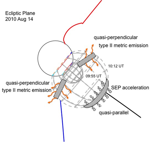
Figure 14. Schematic of the large-scale structure of the shock projected into the ecliptic plane at ∼09:55 UT (inner ellipsoid) and at 10:12 UT (outer ellipsoid) on 2010 August 14 illustrating the regions of the shock front where metric type II emission most likely occurred (i.e., at the lower portions of the shock propagating at low altitudes through denser regions of the corona where quasi-perpendicular conditions were more likely to occur) and where the acceleration of the SEPs observed at L1 most likely occurred (i.e., at the nose of the shock where quasi-parallel conditions and fast speeds were observed).
Download figure:
Standard image High-resolution image
7.4. SEP Transport Mechanisms
Even if the magnetic connection between a particle source and a spacecraft can be perfectly described, this does not necessarily indicate the path along which particles reach the observing spacecraft. If particles only propagate along magnetic field lines, the detection of SEPs requires a direct magnetic connection between the observing spacecraft and the SEP source. However, if particles can propagate across magnetic field lines, and hence spread in longitude, particles can arrive at the spacecraft in the absence of a direct connection. Since in situ observations do not provide information on SEP transport conditions all along their path from their sources to the observer, we have to rely on SEP transport models that assume reasonable values for the transport parameters.
As described in Section 6, the particle intensity–time profiles observed by the three spacecraft during the 2010 August 14 SEP event can be reasonably reproduced by the SEP transport model outlined there with the assumption of justifiable injection and transport parameters. Although the λ⊥/λ∥ ratio assumed by Dröge et al. (2016) and here is relatively small (0.04), the simultaneous fit of the SEP intensities at the three spacecraft requires both models to use a particle source extended over a broad area and acting over a prolonged time interval (Table 3). The fact that STEREO-A observed isotropic particle intensities and that it initially established magnetic connection with a weak, slow portion of the CME-driven shock, where the particle acceleration efficiency is likely to have been low, suggests that SEPs arrived at this spacecraft mostly via cross-field diffusion in IP space as reproduced by our transport model.
8. Summary and Conclusions
The relative simplicity of the SEP event on 2010 August 14 has allowed us to assess the successes and flaws of several state-of-the-art methods used to (1) identify the location of SEP sources, (2) describe the magnetic connection established between spacecraft and these sources, (3) estimate SEP release times, and (4) evaluate the transport of SEPs between their source and the observing spacecraft. Our overall conclusion is that while these methods are useful for inferring the connections between solar phenomena, SEP sources, and spacecraft observations, there are still uncertainties inherent in these methods that prevent us from pinpointing exactly the connection between SEPs observed at 1 au and their sources at the Sun. Notwithstanding these uncertainties, we conclude that the observations of the 2010 August 14 SEP event are likely to be consistent with the following scenario.
Under the assumption that SEPs are mostly accelerated by shocks that are initially driven by CMEs, and that SEPs propagate predominantly along IMF lines, then an interplanetary spacecraft might be expected to detect SEPs only after it has established magnetic connection to a portion of the shock that is accelerating energetic particles. To examine whether this was the case during the 2010 August 14 event, we inferred the shape and speed of the associated shock from EUV and WL images. We then used a coronal magnetic field model to identify the portions of the shock front that were magnetically connected to the STEREO and near-Earth spacecraft, and estimated the shock speed and angle θBn at these locations. We concluded that STEREO-B and near-Earth spacecraft detected SEPs when the portions of the shock connected to these spacecraft acquired high speeds (Figure 10) and quasi-parallel configurations (Table 2), conditions likely to be favorable for SEP acceleration via DSA (e.g., Lee 1983). (The acceleration efficiency will also be determined by other parameters such as shock strength, which depends on the medium through which the shock is propagating. In particular, we note that Salas-Matamoros et al. 2016 and Rouillard et al. 2016 have recently developed techniques to estimate the strength of shocks.) The cobpoints for these two spacecraft were already at relatively high altitudes at this time (>2 R⊙ above the solar surface; cf. Table 2). In contrast, the portion of the fitted shock connected to STEREO-A never reached high speeds (Figure 10(c)), the particle release time is poorly defined and cannot be compared with the field line-shock connection time, and the particles arriving during particle onset at this spacecraft were isotropic. We suggest that the particle increase at STEREO-A was due to SEPs arriving mostly via cross-field diffusion. A simulation of this event using a particle transport model which is consistent with observations has been presented.
We postulate that the regions of the shock front responsible for the acceleration of SEPs were different from those responsible for the metric type II radio burst observed in this event (see Figure 14). Whereas type II radio bursts were generated at lower altitudes on the flanks of the CME shock where quasi-perpendicular geometries were more likely, SEPs were accelerated at higher altitudes when the shock reached high speeds and quasi-parallel geometries.
Unusually for an extended SEP event observed at both STEREO spacecraft and at Earth (e.g., Richardson et al. 2014), the 2010 August 14 event was not accompanied by clear DH type II radio emissions detected by the Wind or STEREO spacecraft, and no event is reported in the Wind/STEREO type II event lists. Close examination of the radio spectra shows only very brief blobs or islands of emission that could perhaps be weak evidence of DH type II emissions (Figure 5). Type II emissions occur when both the shock configuration and conditions in the upstream medium are appropriate, in particular quasi-perpendicular shock, large magnetic field ratio, and high upstream electron densities favor this radio emission (e.g., Knock et al. 2003; Cairns & Schmidt 2015; Schmidt & Cairns 2016, and references therein). The near absence of DH type II emissions in the 2010 August 14 event suggests that these conditions were not met in the IP medium, possibly because (1) the quiet pre-event conditions precluded the presence of denser upstream regions produced by prior events, and (2) the only fast portion of the shock was located near the nose, lasted for only a short period of time (Figure 10(b)), and was quasi-parallel. The in situ detection of an IP shock most likely associated with this event at STEREO-A and near Earth demonstrates that the lack of a DH type II burst is not inconsistent with the presence of an IP shock (e.g., Gopalswamy et al. 2010), although the SEP intensity–time profiles in Figures 1(c)–(d) suggest that the shock was not accelerating particles efficiently when it arrived at 1 au.
We have also demonstrated for the 2010 August 14 event that the extent of the EUV wave propagating over the solar disk (in particular, the lack of evidence for the arrival of the EUV wave front at the footpoint of STEREO-A, which detected a particle event; cf. Figure 6) is not representative of the extent of the SEP event in the heliosphere, reinforcing the similar conclusions of, e.g., Posner et al. (1997), Prise et al. (2014), Lario et al. (2014, 2016), and Kouloumvakos et al. (2016).
Although the scenario outlined above assumes that all particle acceleration occurs at the CME-driven shocks, we do not exclude the possibility that other acceleration processes may have contributed. In particular, the observation of type III radio bursts (Figure 5) indicates the escape of electrons that may have been accelerated by reconnection processes at the time of the flare and following the eruption of the CME. Similarly, SEPs accelerated by the same processes may also have been released into the IP medium. However, cross-field diffusive transport in the corona or IP space would then have to be efficient enough to explain the large spread of SEPs in heliolongitude. We have shown that a transport model simulation including cross-field diffusion can explain the observation of an isotropic particle increase at STEREO-A and can also account for the particle observations at STEREO-B and the Earth (Section 6). However, this requires an extended, prolonged duration, particle source.
In conclusion, the observations of the 2010 August 14 SEP event discussed here again demonstrate how multi-spacecraft observations of SEP events at distant locations provide constraints to proposed scenarios of particle acceleration and transport. In addition, the various uncertainties addressed in this paper suggest that we are still in the early stages of being able to determine accurately the connectivity between SEP sources and interplanetary spacecraft, a necessary step in successfully forecasting the arrival of SEPs at any point in the inner heliosphere.
The present work was performed within the framework of the NASA Living With a Star Targeted Research and Technology (TR&T) Focused Science Topic "Physics-based methods to predict connectivity of SEP sources to points in the inner heliosphere, tested by location, timing, and longitudinal separation of SEPs." D.L. and N.E.R. acknowledge support from NASA LWS TR&T grant NNX15AD03G and NASA HGI grant NNX16AF73G. H.X. was partially supported by NASA LWS TR&T program NNX15AB70G. P.A.M. and N.T. acknowledge support from NASA grant NNX15AB77G. M.L.M. and H.M.B. acknowledge the support of NASA LWS grant NNX15AB80G. M.Z. acknowledges the support of NASA LWS grant NNX15AB76G. L.Z. was partially supported by NSF SHINE grant AGS-1156056. R.Y.K. acknowledges the support from the Office of Naval Research and George Mason University. B.J.T., I.G.R., and T.T.v.R. acknowledge support from NASA grant NNG06EO90A. We thank the STEREO PLASTIC, IMPACT, SECCHI, S/WAVES; SOHO LASCO, EIT, ERNE, EPHIN; ACE EPAM, MAG, SWICS; Wind WAVES; and SDO AIA, HMI teams for providing the data used in this paper. The SDO/AIA and SDO/HMI data are provided by the Joint Science Operations Center (JSOC) Science Data Processing (SDP). The STEREO/SECCHI data are produced by an international consortium of the NRL (USA), LMSAL (USA), NASA-GSFC (USA), RAL (UK), University of Birmingham (UK), MPS (Germany), CSL (Belgium), IOTA (France), and IAS (France). SOHO is a mission of international cooperation between ESA and NASA. The ACE data are provided by the ACE Science Center and the Wind data by the Coordinated Data Analysis Web. We acknowledge Janvier Wijaya (PredSci) for providing MAS model results. We acknowledge the constructive input received from the reviewer.