 Alexandre Belleflamme1,2*
 Klaus Goergen1,2
 Niklas Wagner1,2
 Stefan Kollet1,2Sebastian Bathiany3,4
 Juliane El Zohbi3
 Diana Rechid3
 Jan Vanderborght1
 Harry Vereecken1
- 1Institute of Bio- and Geosciences (IBG-3, Agrosphere), Forschungszentrum Jülich, Jülich, Germany
- 2Centre for High-Performance Scientific Computing in Terrestrial Systems, Geoverbund ABC/J, Jülich, Germany
- 3Climate Service Center Germany (GERICS), Helmholtz-Zentrum Hereon, Hamburg, Germany
- 4Earth System Modelling, School of Engineering and Design, Technical University of Munich, Munich, Germany
In the context of the repeated droughts that have affected central Europe over the last years (2018–2020, 2022), climate-resilient management of water resources, based on timely information about the current state of the terrestrial water cycle and forecasts of its evolution, has gained an increasing importance. To achieve this, we propose a new setup for simulations of the terrestrial water cycle using the integrated hydrological model ParFlow/CLM at high spatial and temporal resolution (i.e., 0.611 km, hourly time step) over Germany and the neighboring regions. We show that this setup can be used as a basis for a monitoring and forecasting system that aims to provide stakeholders from many sectors, but especially agriculture, with diagnostics and indicators highlighting different aspects of subsurface water states and fluxes, such as subsurface water storage, seepage water, capillary rise, or fraction of plant available water for different (root-)depths. The validation of the new simulation setup with observation-based data monthly over the period 2011–2020 yields good results for all major components of the terrestrial water cycle analyzed here, i.e., volumetric soil moisture, evapotranspiration, water table depth, and river discharge. As this setup relies on a standardized grid definition and recent globally available static fields and parameters (e.g., topography, soil hydraulic properties, land cover), the workflow could easily be transferred to many regions of the Earth, including sparsely gauged regions, since ParFlow/CLM does not require calibration.
1. Introduction
Monitoring and forecasting the terrestrial water cycle, and in particular the subsurface water states and fluxes, are increasingly relevant for many sectors, especially for agriculture, e.g., for estimating water availability, groundwater recharge, and water stress for plants, eventually influencing irrigation decision-making, for characterizing the workability and trafficability of fields, and for evaluating leaching of pesticides and fertilizers (Babaeian et al., 2019). Stakeholders from the agricultural sector cope with the interplay between their measures to adapt to or mitigate the impacts of extreme weather events, global warming, optimized and sustainable management practices, market imperatives, and environmental policy constraints (Klages et al., 2020). For example, monitoring and forecasting seepage water may serve two goals. It helps to gauge if nutrients might leach out of the root zone after fertilization, thus becoming unavailable for the plants, and it helps to assess leaching to groundwater resources whose protection is targeted by environmental policies (Knoll et al., 2020; Wendland et al., 2020).
In addition, a soil moisture deficit during spring has been observed in central Europe for more than 10 years (Ionita et al., 2020). Droughts affected the same region in 2018, 2019, 2020, and 2022 during the spring-to-summer vegetation period (e.g., Boergens et al., 2020). These circumstances emphasize the need for a monitoring and forecasting system of terrestrial water resources at the high spatial resolution, eventually contributing to a digital twin that enables a representation, e.g., of local variations in groundwater levels or inter-field dynamics of subsurface water flow (Pylianidis et al., 2021). Especially stakeholders from the agricultural sector (e.g., farmers, advisers, plant breeders, and cooperatives) increasingly have to deal with extreme weather events like droughts that affect crop growth and yield, and soil and water resources (Rosenzweig et al., 2001; Naumann et al., 2021). For example, Brás et al. (2021) showed that drought impacts on crop yield tripled over the last decades in Europe. Cropland and grassland are particularly affected by droughts resulting in major yield reduction (Ciais et al., 2005; Reinermann et al., 2019). Consecutive droughts are even more problematic, because a sufficient recovery of the subsurface water resources is not possible between the events, increasing their impacts from year to year (Rosenzweig et al., 2001; Hartick et al., 2021; Moravec et al., 2021). For example, the meteorological drought (i.e., precipitation deficit over several weeks to months) that affected central Europe in 2019 was less pronounced than in 2018, but the subsurface water deficit increased even more leading to a more severe agricultural drought than in 2018 (Boergens et al., 2020), emphasizing the importance of characterizing droughts based on soil hydrological processes. Future projections show an increase in frequency, duration, and spatial extent for both meteorological (Spinoni et al., 2020) and soil moisture (Grillakis, 2019) droughts in Europe—and particularly eastern and southern Europe—even for scenarios with a strong limitation of greenhouse gas emissions. Multi-year and consecutive drought events are also projected to become more frequent, last longer, and affect larger areas over the next decades in central Europe (Samaniego et al., 2018; Hari et al., 2020), regardless of the climate change scenario and even for scenarios meeting the goal of the Paris agreement to limit the global temperature increase from 1.5°C to 2°C (Lehner et al., 2017).
In that context, hydrological models are increasingly used for prototypical or even operational monitoring of droughts or, more generally, subsurface water deficit and the associated impacts, e.g., on water stress for plants (Dasgupta et al., 2023). Prominent examples are the German (Zink et al., 2016), Czech (Trnka et al., 2020), and Swiss (Zappa et al., 2014) drought monitors. Beyond the monitoring providing information about the evolution of the subsurface water deficit over the last few weeks or even months, the latter two examples also provide short-term forecasts (5–10 days in advance) and even subseasonal outlooks. To meet their societal aim of providing information on stakeholder relevant scales, the hydrological models behind these drought monitors run at the high spatial resolution, ranging from 4 km down to 0.5 km or even 0.2 km for selected catchments of the Swiss drought monitor.
On a subseasonal to seasonal time scale, hydrological modeling approaches predicting the subsurface water budget are increasingly developed with the overall aim of improving the prediction of subsurface water resources and droughts (Dasgupta et al., 2023). For example, some studies analyze the added value of seasonal soil moisture drought predictions obtained by forcing a conceptual hydrological model with numerical weather predictions in comparison with ensemble discharge predictions using historical meteorological data (e.g., Thober et al., 2015) or a climatology (e.g., Bogner et al., 2018). Other studies highlight the importance of factors like snow or temperature on the predictability of soil moisture, e.g., Orth and Seneviratne (2013) over Switzerland, Penland et al. (2021) over California, and Singla et al. (2012) over France. Recently, the European Commission and the Copernicus Climate Change Service (C3S) supported a demonstrator project, EDgE (End-to-end -Demonstrator for improved decision-making in the water sector in Europe), that aimed to provide pan-European, high-resolution seasonal forecasts and climate projections of user-tailored products, including information on the uncertainty, using a multi-model approach, to support decision-making in the water sector (Samaniego et al., 2019; Wanders et al., 2019).
In this context, we developed and operated a simulation setup (called hereafter DE06, as it is centered over Germany with a resolution of 0.611 km × 0.611 km) based on the established hydrological model ParFlow/CLM that allows for the representation of the surface and 3D subsurface hydrodynamics as well as the atmosphere–land surface interactions at a high spatial and temporal resolution over central Europe. DE06 has been designed and implemented with the following objectives:
- To provide relevant information to stakeholders about all components of the terrestrial water cycle, such as diagnostics on the (1) water table depth and groundwater recharge, allowing, for example, the monitoring of the recovery of subsurface water resources after a drought; (2) soil moisture in the root zone, delivering information on water stress for plants, and thus irrigation requirements, but also on the workability and trafficability of agricultural fields; and (3) water fluxes in the unsaturated zone providing support for estimating the leakage of nutrients and pollutants into deeper soil layers and even into the groundwater. As explained below, the modeling system presented here calculates the water state and fluxes in a three-dimensional matrix ranging from the surface and the variably saturated zone to the groundwater, which allows us to derive any diagnostics based on soil water and shallow groundwater within the model's vertical extent.
- To allow for an efficient quasi-operational computation of daily short-term forecasts with a lead time of up to 10 days, including a representative ensemble for estimating the impact of the driving atmospheric conditions and their uncertainty on the subsurface water budget, but also for probabilistic ensemble predictions on subseasonal to seasonal timescales, thus providing information that may be utilized to support stakeholder decisions based, e.g., on the diagnostics explained above.
- To allow for the calculation of a reference time series over the past years to analyze recent hydrometeorological extremes and their impacts on the subsurface water budget and the parameters explained above, and to put the forecasts in a climatological context (e.g., through anomalies).
- To be usable as a stand-alone hydrological model system of the variably saturated zone directly driven by a few near-surface atmospheric parameters, but also offering the possibility of being integrated as a hydrological module in a fully coupled terrestrial modeling platform, e.g., via a coupling with a regional atmospheric model and a land surface model.
This study serves four goals: (i) to present the DE06 setup; (ii) to present the subsurface water resources monitoring and forecasting system relying on DE06; (iii) to show validation results of some key terrestrial water cycle components relevant to stakeholders and their requirements; and (iv) to present prototypical applications, and information products, of the new quasi-operational, prototypical setup.
This study has the following structure: Section 2 presents the DE06 simulation setup and configuration in detail and explains how the static fields for the model parameterization were generated; Section 3 presents the monitoring and forecasting system based on DE06, the different types of simulations that are performed, their atmospheric forcing, and their initialization; Section 4 presents a comparison of the simulated reference time series with observational data for four relevant variables of the subsurface water budget; Section 5 presents an application example of DE06 in forecast mode, aimed to provide information on the subsurface water resources; and finally, Section 6 presents the conclusion.
2. Methodology
2.1. ParFlow/CLM
In this study, we use the integrated hydrological model (IHM) ParFlow v3.8.0. ParFlow is a parallel fully coupled model that uses partial differential equations (PDE) to simulate unsaturated and groundwater flow, as well as surface flow (Maxwell et al., 2016; Kuffour et al., 2020) in a continuum approach. The variably saturated subsurface flow is calculated with the Richards equation, and the kinematic wave equation is applied to calculate overland flow (Kollet and Maxwell, 2006). Topography is represented through a terrain-following grid (Kuffour et al., 2020). The water retention and hydraulic conductivity curves as key soil hydraulic properties are described by the Mualem–van Genuchten functions (Van Genuchten, 1980), and their parameters are estimated with pedotransfer functions. An important advantage of physics-based IHMs as opposed to lumped hydrological models is that they do not require extensive calibration steps to produce robust results (Poméon et al., 2020; Saadi et al., 2023a). For example, using the DE06 setup presented here, Saadi et al. (2023a) showed that, even without calibration, ParFlow gives similar results compared to a calibrated lumped model, for the discharge during the extreme flooding event of mid-July 2021 in western Germany.
Over the last 15 years, ParFlow has become a well-established simulation platform among the integrated, physics-based models, used in different setups, for many model domains and applications. For example, it has been used for theoretical hydrodynamic exercises and sensitivity studies (e.g., Maxwell and Kollet, 2008a; Frei et al., 2009; Kollet, 2009; Schalge et al., 2019; Maina et al., 2020; Schreiner-McGraw and Ajami, 2020), model intercomparisons (Maxwell et al., 2014; Koch et al., 2016), watershed hydrodynamics and hydrological scaling (Maxwell and Kollet, 2008b; Rahman et al., 2014; Fang et al., 2015), and as the hydrological component in the fully coupled Terrestrial Systems Modelling Platform (TSMP), both for analyses and sensitivity assessments at the climatic scale (Keune et al., 2016, 2018; Furusho-Percot et al., 2019, 2022; Hartick et al., 2021), and within prototypical forecasting systems (Kollet et al., 2018). ParFlow is also applied to perform high-resolution simulations at continental scale, e.g., at 1 km over a major part of continental North America (Maxwell et al., 2015; O'Neill et al., 2021). Finally, as mentioned above, and even if its primary aim is the monitoring and forecasting of subsurface water resources, DE06 has already been applied in studies related to the unprecedented flood event that affected western Germany and eastern Belgium in mid-July 2021. Saadi et al. (2023a) assessed the effect of different radar-based precipitation products on the simulated hydrological response, and in particular the stream discharge, and Saadi et al. (2023b) analyzed the added value of these products for flood nowcasting.
To represent atmosphere–surface–subsurface interactions, we use the land surface model CLM (Common Land Model) modified by Dai et al. (2003) and integrated as a module into ParFlow (Kuffour et al., 2020). This allows a coupled representation of the water, energy, and momentum exchanges between the surface and the subsurface with the near-surface atmospheric states given as boundary conditions (see below for the atmospheric forcing).
Other boundary conditions, i.e., at the lateral and bottom boundaries of the domain, are all defined as no-flow conditions (O'Neill et al., 2021). Thus, the only source of water is precipitation, and the sinks are evapotranspiration and routing of overland flow out of the domain via rivers. The boundaries are arbitrary and placed at large distances to exclude boundary impacts from the region of interest. To honor flow-through lakes, lake volumes are included as low-conductivity hydrofacies types that are fully saturated in the simulations with ponded water being routed via the overland flow boundary conditions. While this is a simplifying approximation of reality, it constitutes an improvement to previous lake approximations using constant head boundary conditions. Note, the ocean areas are approximated the same way, to relax the assumption of the constant head along the coast line and improve computational efficiency.
To reduce the computational time in the forecast-driven setup, and as the primary goal of DE06 are subsurface water resources instead of discharge, the overland flow routing is not simulated explicitly in most of our simulations (described below in the section about the monitoring and forecasting system). Thus, the discharge, if needed, may be calculated during post-processing using a run-off approach based on the ponding height accumulated over the catchment area for each time step. This implies two simplifications: (1) possible re-infiltration of overland flow further downstream along the river network, at grid points where there might be no exfiltration, is ignored, and (2) calculated discharge is instantaneous, i.e., the delay in the overland flow generation or exfiltration and its measurement at the catchment outlet is ignored.
We run ParFlow/CLM on the GPU (Graphics Processing Unit) compute nodes of the JUWELS Booster high-performance computing (HPC) system at the Jülich Supercomputing Centre (JSC) in Germany. Hokkanen et al. (2021) have implemented software functionalities to efficiently run the model on such accelerated HPC systems. This is a prerequisite to operating ParFlow/CLM in a quasi-operational monitoring and forecasting mode at high resolution over a large model domain (see Section 3). Only a single compute node with four GPUs is needed to run a 10-day forecast in 6–10 h wall clock time, depending on the number of iterations needed by the solver to converge to a solution.
2.2. Model domain and grid
The DE06 ParFlow/CLM setup uses a Cartesian grid with equidistant grid spacing in the lateral direction of 2,000 × 2,000 grid cells with a resolution of 0.0055° × 0.0055° (~ 0.611 km × 0.611 km) covering Germany and the neighboring regions (called hereafter DE-0055). This grid extends over 15 terrain-following vertical model layers. Their thickness increases with depth, the uppermost layer reaching from the surface to 2 cm depth and the lowest layer extending from 42 m to 60 m below the surface.
To facilitate the comparison with other model outputs and data sets, the DE-0055 grid has been defined as a rotated-pole equal area grid inscribed into the widely used EUR-11 grid of the COordinated Regional Downscaling EXperiment (CORDEX) (Gutowski et al., 2016). DE-0055 uses the EUR-11 rotated pole parameters, and the horizontal resolution and the grid edges are defined so that each EUR-11 0.11° grid cell has 20 × 20 DE-0055 grid cells inscribed. As the DE-0055 grid is located near the geographic center of the EUR-11 grid, it is defined in the vicinity of the equator on the rotated grid, where the convergence of the longitudes is almost negligible, so that we can reasonably assume that DE-0055 has equal area grid cells everywhere. The largest difference in grid cell area over the grid is about 0.6%. The grid compatibility also simplifies coupling, e.g., within the TSMP framework, where, e.g., the COSMO atmospheric model uses the EUR-11 grid (Kollet et al., 2018).
The domain extent of the DE-0055 grid meets two main criteria (see Figure 1): (i) large central European river basins, such as the Elbe and Rhine river basins, where many socio-economic activities take place, have to be fully included in the domain. This increases the impact and relevance of the simulations and allows for a comparison of river discharge with other models or observations; and (ii) a margin of at least 200 km, which excludes impacts of the arbitrary lateral no-flow boundary conditions.
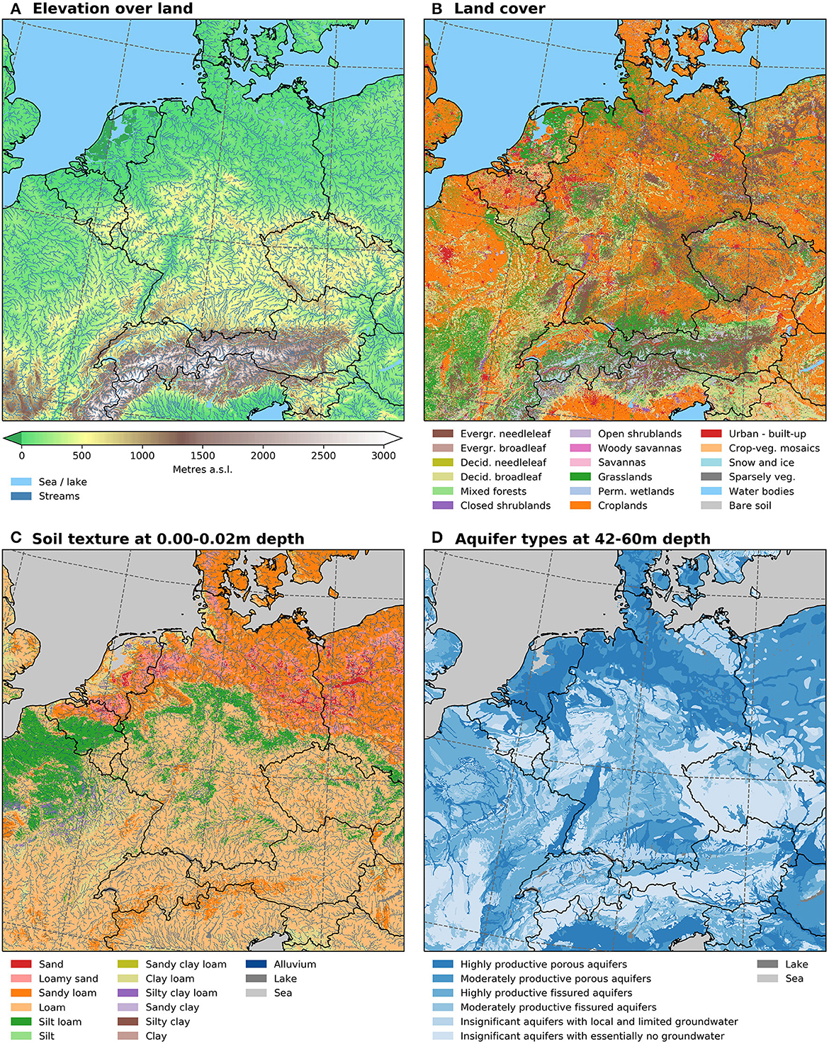
Figure 1. Main static fields utilized in this study as they are regridded on the DE-0055 grid. (A) ASTER GDEM elevation above sea level and imposed streams (blue lines) derived from the hydrological adjusted MERIT DEM used to generate the slopes. (B) IGBP land cover types based on CLC2018. (C) USDA soil texture types based on SoilGrids250m texture data and alluvium for the uppermost layer (0.00–0.02 m depth). (D) IHME aquifer types in the lowest layer (42–60 m depth).
2.3. Static fields—Soil and surface parameterization
To build a realistic heterogeneous model setup, ParFlow requires static fields containing information on the topography and the soil's hydraulic properties. CLM needs information on the land cover and the soil color. To ensure consistency among all static fields, a land–sea mask has also been defined and applied, as the original data sets come from different sources and are characterized by different spatial resolutions. Because the workflow to set up DE06 is aimed to be relocatable to any other region in the world, we exclusively use global databases to generate the static fields and parameters needed by ParFlow/CLM.
2.3.1. Land–lake–sea mask
The land–sea mask has been generated based on Advanced Spaceborne Thermal Emission and Reflection Radiometer (ASTER) Global Digital Elevation Model (GDEM) (Abrams et al., 2020; original resolution 1′′) with the tool EXTPAR (External Parameter for Numerical Weather Prediction and Climate Application) via the web interface WebPEP, developed and made available by the Climate Limited-area Modeling Community (CLM-Community). Using the EXTPAR tool ensures that the model grid and static fields are compatible with the EUR-11 grid specification.
To keep the possibility to assign different hydraulic parameters to “sea” and “lake” grid cells (see below), we have already distinguished them in the mask, thus building a ternary land–lake–sea mask.
2.3.2. Slopes
As we run ParFlow with the terrain-following grid option, topographic slopes derived from a DEM (Digital Elevation Model) are required. These slopes are calculated based on the ASTER GDEM projected onto the DE-0055 grid with the EXTPAR tool as explained above (see the GDEM in Figure 1A), using procedures from the TSMP modeling framework (Shrestha, 2019). The slopes are defined to give a D4 flow direction for each grid cell (i.e., the flow is directed toward N, E, S, or W), meaning that they have a non-zero value either in the x-direction or in the y-direction. The Shrestha (2019) algorithms ensure that each grid cell is drained out of the domain at the domain margin, avoiding the water to concentrate in local depressions, as ParFlow does not handle the overflow. This also leads to the construction of an artificial drainage network in the lakes and seas. Furthermore, to avoid exaggerated drainage and thereby drying along the coasts, we have decreased the slopes over all lakes and seas to the lowest allowed slope value, i.e., |10e-6|, based on the land–lake–sea mask, thus strongly slowing down the water flow, except in the drainage channels to ensure efficient drainage throughout the domain.
As the slopes are calculated based on a DEM, they might lead to wrong river trajectories, especially in flat terrain, in the case of channelized rivers, or regions below sea level. The most notable examples in our domain are the Rhine and Meuse river mouths and the Ijsselmeer region in The Netherlands. The resulting artifacts in the hydrological network are avoided by imposing (or “burning”) the correct river trajectories to the slopes during their computation. Hydrologically adjusted DEMs present an elevation that has been modified so that the resulting hydrological network is correctly located. In DE06, we use the hydrologically adjusted DEM at a 3′′ resolution from the MERIT database (Yamazaki et al., 2019). It has been projected onto the DE-0055 grid by selecting for each DE-0055 grid cell, the lowest elevation value among all nearest neighbors in the MERIT-adjusted DEM. This regridding, as the regridding of almost all static fields explained below, has been performed with the Python package xESMF (https://github.com/pangeo-data/xESMF). The steepness of the slopes is thus calculated with the ASTER DEM, and their direction is corrected using the MERIT-adjusted DEM, where needed.
A visual comparison of the hydrological network built by ParFlow after a few hundred time steps of the first spin-up phase (see below) with the rivers of the HydroSheds database (Lehner et al., 2008) shows a very good agreement besides some local differences (data not shown).
2.3.3. Soil types—Soil hydraulic parameters
To solve the water flow equations in variably saturated porous media, ParFlow needs soil hydraulic parameters to be defined for each grid cell. These parameters are the porosity, the saturated hydraulic conductivity, and the parameters defining the Van Genuchten relationships (Van Genuchten, 1980), i.e., the saturated and residual water content, alpha, and N values.
For the upper layers (soil and regolith), these parameters have been estimated globally in the framework of the Rosetta model (Zhang and Schaap, 2017) for the 12 USDA texture classes. For each grid cell of the DE-0055 grid, we have determined the USDA texture class based on the texture data (sand, silt, and clay fractions) of the global SoilGrids data set v2017 at 250 m resolution (Hengl et al., 2017), which have been bilinearly interpolated on the DE-0055 grid (Figure 1C). Since the SoilGrids texture fractions vary over seven layers from the surface to 2 m depth, they have been linearly interpolated to the depth layers used in DE06. Below 2 m, they are considered constant.
For the deeper layers (in the bedrock), the aquifer types are defined by the six types of the “International Hydrogeological Map of Europe 1:1,500,000” (IHME1500, Duscher et al., 2015, Figure 1D). In DE06, these aquifers are characterized by different saturated hydraulic conductivity values. The transition between the SoilGrids-based USDA texture classes and the IHME1500 aquifers is determined by the depth-to-bedrock information available in the SoilGrids database. Note that the deepest layer, from 42 m to 60 m depth, has IHME1500 aquifers everywhere, regardless of the depth-to-bedrock.
Furthermore, to account for the higher hydraulic conductivity in the river beds, i.e., alluvium, we have superimposed the stream segments of the rivers computed during the slope generation process as a supplementary type above the depth-to-bedrock.
Finally, as explained above, we consider all seas and lakes identified in the land–lake–sea mask as supplementary soil types homogeneous over the entire soil depth and characterized by a very low saturated hydraulic conductivity. As this setup focuses on subsurface water resources, we do not attempt to represent realistically the water states and fluxes in open water bodies. A very low saturated hydraulic conductivity leads to almost no subsurface water fluxes in the lakes and seas. This makes it easier for the solver to converge to a solution. It also ensures that the “soil patches” representing the lakes and seas always remain saturated, which is essential to avoid dry artifacts along the coastlines due to exaggerated drainage into the water bodies; this would happen if they were not saturated.
2.3.4. Land cover
ParFlow's CLM module is based on the 18 IGBP (International Geosphere-Biosphere Programme) land cover types, which are then translated to Plant Functional Types (PFTs) based on parameters like the leaf- and stem-area indices, the roughness length, and leaf and stem visible and near-infrared reflectance and transmittance.
In DE06, we chose to use the Europe-wide Corine Land Cover CLC2018 v20 data set available at a resolution of 100 m (Corine Land Cover, 2018). First, we converted the 44 CLC2018 land cover types to the 18 IGBP types. Then, we regridded the resulting land cover onto the DE-0055 grid with the k-nearest neighbor method, meaning that the most frequent land cover type among the nearest neighbors of a given DE-0055 grid cell is attributed to this cell (Figure 1B). Note that the IGBP types “permanent wetlands” and “snow and ice” are not supported by ParFlow/CLM, thus we have replaced these land cover types with “grasslands” and “barren or sparsely vegetated,” respectively.
2.3.5. Soil color
For calculating the radiation budget, CLM also needs the soil color to be split into eight classes following the IGBP definition. For each soil color class, albedo values depending on radiation (short vs. long-wave) and soil moisture (dry vs. wet) are defined in the CLM parametrization. Here, we use the global soil color v2008 data set from the Community Land Model and available at 0.5° resolution, which we reduced from 20 to 8 classes.
3. Monitoring and forecasting system
3.1. Atmospheric forcing
ParFlow/CLM requires eight surface and near-surface atmospheric parameters as forcing (names in CMOR standard): near-surface air temperature (tas), specific humidity (huss), meridional (vas) and zonal (uas) wind speed components, surface air pressure (ps), total precipitation (pr), and visible (rsds) and infrared (rlds) downward radiation at the surface. Here, we use the near-surface parameters at their standard height, i.e., 2 m for air temperature and specific humidity and 10 m for wind speed.
Since the main purpose of DE06 is to generate forecasts of the subsurface water budget, we use several weather forecast products from the ECMWF (European Centre for Medium-Range Weather Forecasts) (Owens and Hewson, 2018): the deterministic medium-range forecast HRES, the probabilistic medium-range 50-member ensemble forecast ENS, and the probabilistic seasonal 50-member ensemble forecast SEAS. The ParFlow/CLM simulations performed with these data are presented in more detail below. All ECMWF data are downloaded at the initial resolution of HRES, i.e., 0.1° × 0.1° (~11 km). They are then projected onto the DE-0055 grid with the CDO (Climate Data Operators) bicubic remapping tool (Schulzweida, 2021). We also make use of CDO to interpolate the data to an hourly time step when they are only available at a 3- or even 6-h time step. Note that as the specific humidity at 2 m is not available as HRES output, we calculate it based on the dew point at 2 m and the surface air pressure following the equation of Bolton (1980) before the regridding.
Maina et al. (2020) analyzed the sensitivity of ParFlow/CLM simulation results to the resolution of the atmospheric forcing for a watershed located in northern California. This watershed compares very well with the DE-0055 domain, both in its resolution and in the complexity and heterogeneity of the simulated region, as it extends from a mountain range to a wide fluvial plain, with heterogeneous soil and land cover properties. Based on their conclusions, we can assume that the main spatial patterns and temporal evolution of the hydrological processes might be well-captured, even with an atmospheric forcing resolution of about 11 km. The largest biases due to the atmospheric forcing resolution would appear (i) in relation to the snow accumulation and melt, especially in mountainous regions like the Alps, and (ii) for a short time period during and after local precipitation events like rain showers.
3.2. Initialization of the simulation
Because we do not know a priori the state of the subsurface water budget, and particularly the depth of the groundwater table, at the very beginning of the simulation period, the simulation has to be spun-up first. This means that it is started with arbitrary initial conditions and is then run over a longer period to progressively reach a dynamical equilibrium. As this equilibrium is reached by the system based on the physical equations governing the terrestrial water cycle and on the properties (soil hydraulic parameters, elevation, land cover, etc.) of the surface and subsurface, no calibration is required.
For this simulation, the spin-up started with an almost homogeneous, idealized setup. Its complexity was gradually increased by introducing the heterogeneous static fields and forcings (here ECMWF HRES) described above. Figure 2 shows the step-by-step spin-up evolution, where each step was retained until the model system reached an intermediate equilibrium. Gradually stepping up the simulations' complexity has two reasons:
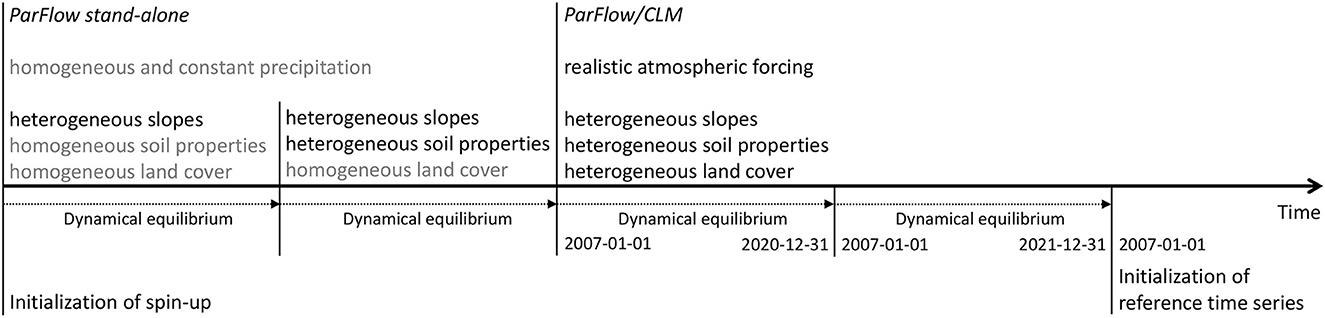
Figure 2. Flowchart summarizing the main steps of the gradual spin-up, from a simplified homogeneous ParFlow stand-alone setup to a coupled ParFlow/CLM heterogeneous setup with real data atmospheric forcing. Gray font color indicates homogeneous or idealized forcings and parameters that have been replaced by heterogeneous and more realistic ones during the spin-up phase.
(i) Inserting the heterogeneous static fields progressively makes it easier to track and identify artifacts and inconsistencies that these fields might introduce into the simulation. Especially during the spin-up with idealized atmospheric forcing (i.e., constant precipitation), it is easier to identify artifacts, e.g., due to the interplay of the slopes and the soil hydraulic properties, or to verify that the river network is realistic (similar to a parking lot experiment). These artifacts can then be corrected without having to re-run the spin-up from the beginning.
(ii) As ParFlow uses an iterative PDE solver, a solution is difficult when starting with fully heterogeneous static fields. It would then have to reconcile an oversimplified subsurface water state far from equilibrium with complex, heterogeneous fields. The complexity of the system would be even more accentuated through the heterogeneous atmospheric forcing, especially when the infiltration rate is high, e.g., due to snow melt or heavy rain. A progressive complexification of the system allows us to gradually move from the very idealized and unrealistic initial condition to a more complex and realistic situation.
3.3. Monitoring and forecasting system—simulations
Relying on the ParFlow/CLM model setup and the atmospheric forcing data described in the previous sections, we developed a monitoring and forecasting system of the terrestrial water cycle over Germany and the neighboring regions consisting of the following five simulations.
- A deterministic medium-range forecast is run every day, driven by ECMWF HRES data over the whole available forecast period, i.e., 240 h. Note that for practical reasons of data availability and our forecast clock, we use the HRES forecast initialized at 12 UTC.
- A 50-member ensemble medium-range forecast forced with ECMWF ENS is performed over the same lead time (i.e., 240 h) to assess the uncertainty related to the weather forecast, especially the precipitation. Note that we calculate this ensemble every 2 days to limit computational costs and hence energy consumption. The inertia of the system from one day to another warrants this approach.
- At the beginning of each meteorological season, a probabilistic 50-member ensemble seasonal forecast driven by ECMWF SEAS is calculated over the entire SEAS forecast period, i.e., 7 months.
- A reference time series starting on 01 January 2007 is prolonged by 24 h every day (last step in Figure 2). This reference simulation provides the initial conditions for all forecast simulations presented above. Thus, to ensure consistency between this time series and the forecasts, we chose to drive it with HRES rather than a reanalysis such as ERA5, even if we are aware that the Integrated Forecasting System (IFS) model from ECMWF, which is utilized to calculate the weather forecasts we use, is evolving. Hence, our reference time series simply consists of ParFlow/CLM simulations driven by the first 24 h of each daily HRES forecast.
- As explained in the Methodology section, all simulations listed above are run without explicit calculation of the overland flow routing, mainly to reduce the computing time. Nevertheless, a second reference time series is calculated every day since 2021, again driven by the first 24 h of each daily HRES forecast, but with an explicit calculation of the overland flow routing. Even if DE06 is primarily aimed at subsurface water resources monitoring and forecasting, this simulation allows us to easily recalculate a forecast with overland flow if this is of interest regarding the hydrometeorological situation. If we would have to initialize a forecast with explicit overland flow calculation from the reference time series without overland flow, we would first need to run a spin-up of several months.
Note that this monitoring and forecasting system enables integration of observation-based precipitation fields, e.g., radar precipitation data, as replacement of the HRES precipitation as forcing for the reference time series. This allows us to build the time series based on more realistic and spatially and temporally detailed precipitation data than those given by HRES. However, we did not make use of this capability to compute the reference time series used for the comparison with observational data described in the next section.
It is also important to note that ParFlow is technically able to account for anthropogenic processes like groundwater pumping or irrigation. Nevertheless, the monitoring and forecasting system described here is based on a model setup without any human interventions with the terrestrial water cycle. In fact, including these processes would require (near) real-time information, e.g., on the pumping rate and depth or on the location, time, and amount of irrigation, which is not available. Also, infrastructural alterations of the river network such as barrages, dams, and man-made lakes are not included.
4. Validation with observational data
In this section, we validate our reference time series described above over the period 2011–2020 with observation-based data sets covering all important components of the surface and subsurface water budget, namely near-surface volumetric soil moisture, water table depth, evapotranspiration, and discharge.
To provide a consistent evaluation among the aforementioned variables, we decided to focus the comparison on monthly mean anomalies, i.e., monthly mean values from which the long-term average of the considered month over the whole comparison period has been subtracted. Two comparison metrics, namely the Pearson correlation coefficient and the root-mean-square error (RMSE), are calculated for these monthly mean anomalies. This allows a focus on the temporal dynamics of the system, but also on the ability of DE06 to adequately represent the specificities of each month, as (i) some of the observational data cannot be used directly to compare absolute values, and (ii) this allows an analysis beyond the seasonal cycle, which is very pronounced for most of the variables analyzed here. Nevertheless, the ability of DE06 to reproduce the seasonal cycle is shown via several time series of zero-centered monthly means, i.e., monthly means from which the long-term average over the whole period has been subtracted. The only exception is discharge, for which we present the widely used Nash–Sutcliffe and Kling–Gupta efficiency scores calculated based on absolute monthly mean values, in addition to the correlation on the monthly mean anomalies.
4.1. Volumetric soil moisture
To validate our results over the whole simulation domain, we compared the volumetric soil moisture (volSM) simulated by ParFlow/CLM with the satellite-based ESA CCI (European Space Agency Climate Change Initiative) combined daily soil moisture product v06.1 (Dorigo et al., 2017; Gruber et al., 2019). For the comparison, monthly data for the common time period 2011–2020 are used. The ParFlow/CLM data from the uppermost layer (0–2 cm depth) are aggregated to the coarser ESA CCI grid (resolution of 0.25°) by averaging all nearest neighbor DE-0055 grid cells for each ESA CCI grid cell, as the soil moisture can only be derived from satellite observations for the few uppermost centimeters. As stated in Dorigo et al. (2015), ESA CCI volSM is scaled against the GLDAS-Noah land surface model (LSM) and thus it cannot be considered an independent data set for comparing absolute values and assessing model biases. Therefore, we focus our analysis on the temporal dynamics and monthly anomalies.
The Pearson correlation coefficient between the monthly volSM anomalies of ParFlow/CLM and ESA CCI shows values above 0.5 over 80% of the simulation domain, which indicates that DE06 can reproduce the observed near-surface soil moisture (Figure 3A). We consider these as good results, especially since (i) the atmospheric forcing used for the simulations, i.e., the deterministic forecast HRES from ECMWF, adds more uncertainty compared to, e.g., a reanalysis that integrates a large number of observations, and (ii) DE06 has not been calibrated with any observational data. The correlation values obtained here are of the same order of magnitude or even higher than those obtained by Dorigo et al. (2017) over the same region when comparing a previous version of the ESA CCI combined product (v03.2) with soil moisture from the ERA-Interim reanalysis. The lower correlation over the Alps can be explained by the frozen soil that is not taken into account in DE06. This leads to a dry bias during winter, when the soil water continues to percolate, while there is no recharging infiltration as the precipitation accumulates as snow on the surface. Furthermore, this joins the conclusion of Maina et al. (2020) stating that a coarser resolution of the atmospheric forcing mainly influences surface and subsurface processes and states as they are directly linked to the atmosphere, and that this is particularly the case in mountainous regions.
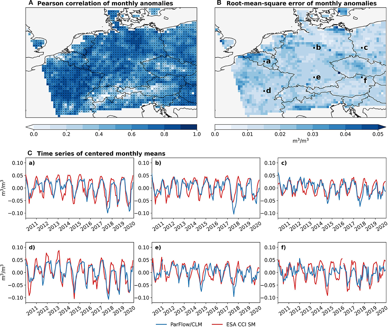
Figure 3. Comparison of the monthly volumetric soil moisture simulated by ParFlow/CLM for the uppermost 2 cm and regridded on the ESA CCI grid and the ESA CCI soil moisture over 2011–2020. (A) Pearson correlation coefficient of the monthly mean anomalies (colors). Black dots indicate ESA CCI grid cells where the correlation is statistically significant (p-value < 0.01). (B) Root-mean-square error of the monthly mean anomalies (RMSEa), in m3/m3. (C)(a)–(f) Time series of zero-centered monthly mean volumetric soil moisture anomalies for six arbitrary selected grid cells marked on the map in (B), in m3/m3.
The root-mean-square error of the anomalies (RMSEa), which is widely employed to evaluate soil moisture (e.g., Dorigo et al., 2015; Zhu et al., 2019; Gruber et al., 2020) and which we define as the RMSE calculated over the monthly anomalies, shows good results over the region (Figure 3B). It does not present a clear spatial pattern, and with an average of 0.02 m3/m3, it lies even below the uncertainty of the ESA CCI combined product for which Dorigo et al. (2015) obtained values between 0.03 and 0.09 m3/m3 on a global comparison with 596 in situ measurement time series.
Finally, a visual comparison of zero-centered monthly mean time series for some selected grid cells also shows good agreement between the two data sets (Figure 3C). It is interesting to see that the amplitudes of the seasonal cycles of volSM match closely, even if DE06 tends to underestimate the drought years, especially 2018, compared to ESA CCI.
4.2. Evapotranspiration
For the evapotranspiration (ET), we compare the DE06 results from ParFlow's CLM module with the “actual evaporation” (“E”) from GLEAM v3.5a over their common period, i.e., 2011–2020. GLEAM (Global Land Evaporation Amsterdam Model) calculates different evaporation terms daily at 0.25° resolution using satellite and reanalysis data as forcing and via data assimilation (Miralles et al., 2011; Martens et al., 2017). The “actual evaporation” from GLEAM corresponds to the sum of all evaporative terms, i.e., transpiration, bare-soil evaporation, open-water evaporation, interception loss, and snow sublimation (Miralles et al., 2011). As for volSM, the simulation results are aggregated by averaging all DE-0055 nearest neighbors on the coarser GLEAM grid.
The Pearson correlation coefficient calculated on the monthly mean anomalies lies above 0.5 over 86% of the domain, indicating that DE06 can represent ET from GLEAM (Figure 4A). This is confirmed by a visual comparison of the time series of zero-centered monthly means for some selected grid cells (Figure 4C). These time series also highlight the ability of ParFlow/CLM to reproduce the seasonal cycle. The RMSEa also confirms the good results with an average of 0.15 mm/day over the domain (Figure 4B). The slightly higher RMSEa values, associated with a lower Pearson correlation, are observed over the Alps, where ParFlow/CLM underestimates ET compared to GLEAM, especially in summer (not shown). This might be due to different parameterizations controlling the snowmelt, but the different resolutions might also influence the results in such regions with complex terrain. As for volSM, this agrees with the observations of Maina et al. (2020), as ET is directly dependent on the atmospheric forcing and thus more sensitive to the impact of its coarser resolution than, e.g., water table depth (see next section).
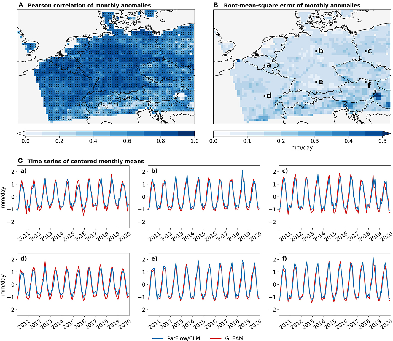
Figure 4. Comparison of the monthly actual evapotranspiration simulated by ParFlow/CLM and regridded on the GLEAM grid and the GLEAM actual evaporation over 2011–2020. (A) Pearson correlation coefficient of the monthly mean anomaly (colors). Black dots indicate GLEAM grid cells where the correlation is statistically significant (p-value < 0.01). (B) Root-mean-square error of the monthly mean evapotranspiration anomaly, in mm/day. (C)(a)–(f) Time series of zero-centered monthly mean evapotranspiration for six arbitrary selected grid cells marked on the map in (B), in mm/day.
4.3. Water table depth
For the comparison of the water table depth (WTD), we used monthly WTD measurements collected from several German states and neighboring countries and processed by Ma et al. (2022). The observed time series are available until 2016 so the comparison period is 2011–2016. They are assigned to the nearest DE-0055 grid cell. If one grid cell contains more than one WTD well, the monthly average over all wells is used, resulting in 5799 grid cells with WTD observations.
As for volSM, we cannot compare the absolute WTD values and calculate, e.g., biases, as (i) some measurements do not give the water table depth from the surface, but the groundwater level above the reference sea level and we do not know the exact altitude of these wells to calculate the water table depth, and (ii) even at a high resolution of 0.611 km × 0.611 km, local conditions might lead to large discrepancies between observed and modeled absolute WTD values. Thus, we concentrate our analysis on the temporal dynamics and monthly mean anomalies.
The Pearson correlation coefficient calculated using the monthly mean anomalies shows good results over wide parts of the domain, with values above 0.5 for 49% of the wells, regardless of the soil properties (Figure 5A). A more detailed analysis shows that the correlation presents much higher values when considering only shallow groundwater bodies, where the WTD dynamics might be more tightly coupled to surface exchange processes and a result of surface–subsurface hydrodynamics. The correlation coefficient reaches 0.47 on average for WTD < 5 m. It has still an average value of 0.38 where WTD is between 5 m and 10 m, and it drops to an average of 0.14 where WTD is deeper than 10 m. This can be explained by the less marked connection of deeper groundwater bodies with the driving source-sink term, i.e., precipitation-evapotranspiration, on one side, and the stronger influence of geological features, such as preferential flow directions, which are not accounted for in DE06.
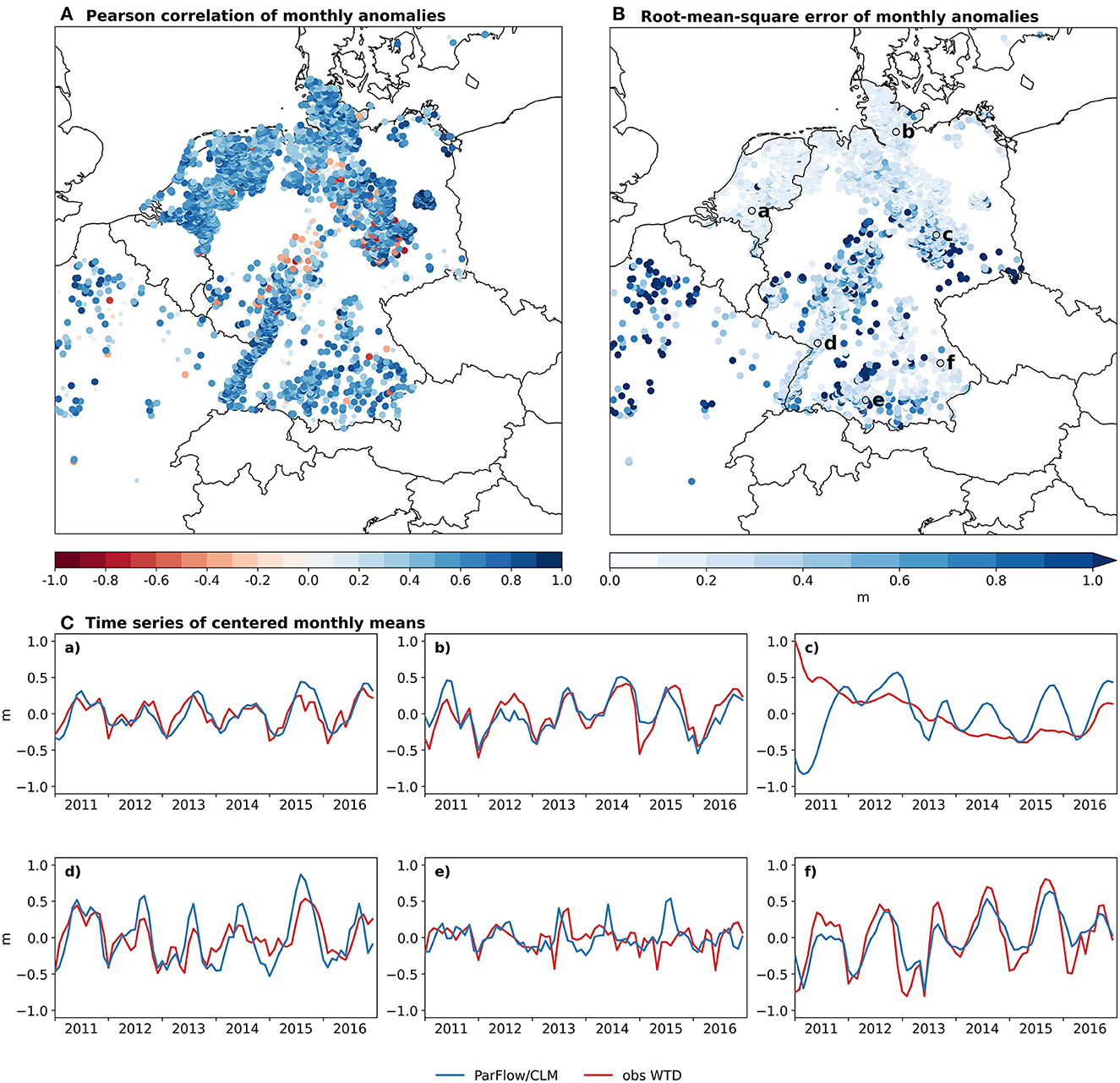
Figure 5. (A) Pearson correlation coefficient between the monthly mean water table depth anomaly simulated by ParFlow/CLM and observed monthly water table depth anomaly data over 2011–2016 for all 5,799 grid cells containing observation data. The 4,236 grid cells with a significant correlation coefficient (p-value < 0.01) are depicted by big circles. (B) RMSEa over the same data, in m. (C)(a)–(f) Time series of zero-centered monthly means for six arbitrary selected grid cells marked on the map in (B), in m.
The average RMSEa, calculated again over the monthly mean anomalies, is 0.32 m over all 5,799 grid cells. To put it in perspective, this is much smaller than the average standard deviation of the observed monthly anomalies, which is about 1.37 m. As it appears on the map, most regions present very low RMSEa values, especially in the Netherlands, northern Germany, the Rhine Valley, and Bavaria (Figure 5B). Much higher values are observed, e.g., in France or Saxony. The highest RMSEa values often coincide with non-significant or negative correlation coefficient values and the domain average RMSEa reduces to 0.24 m if only grid cells with a positive and significant correlation are taken into account. It should be noted here that anthropogenic processes, and in particular groundwater pumping, which are not accounted for in DE06, can have a large impact on WTD (O'Neill et al., 2021).
The time series of centered monthly means (Figure 5C) confirm that DE06 is generally able to reproduce the annual cycle and its amplitude, especially for shallow groundwater bodies, as the average WTD simulated by ParFlow/CLM lies below 2 m for all time series, except for Figure 5C(c). Here, the simulated average WTD is around 6 m and the temporal dynamics are overestimated compared to observation, which joins the interpretation of the correlation of the monthly anomalies explained above.
4.4. Discharge
The simulated discharge (Q) is compared with monthly observed river gauge data from GRDC (Global Runoff Data Centre, 56068 Koblenz, Germany). As only little data are already available for 2020, the time series are compared over the 2011–2019 period. For each gauge within the domain providing data over this period, the corresponding catchment on the DE-0055 grid is defined as the catchment with the closest area to the GRDC catchment area for outlets located within a radius of five grid cells around the coordinates of the GRDC outlet. Furthermore, only catchments that are fully included in the domain and for which the area difference between the DE-0055 grid and GRDC is below 20% are retained. As a result, the comparison is made over 231 catchments of various shapes and sizes (ranging from 1.8 to 160,800 km2) including subcatchments of the major rivers such as the Rhine, the Elbe, and the Danube. As explained above, the overland flow routing is not simulated explicitly in the reference time series simulation so Q is calculated afterward using a run-off approach based on the ponding heights in all grid cells at the end of a time step. At the beginning of a time step, all water ponding on the land surface is instantaneously routed to the outlet, and the ponding height at the end of a time step is derived from the simulated flux across the land surface and the difference between precipitation and evaporation from the surface during the time step.
With more than 96% of the gauges presenting a value above 0.5, the Pearson correlation coefficient calculated on the monthly mean anomalies shows a good agreement between the uncalibrated DE06 and the GRDC observations (Figure 6A). These results are confirmed by the statistics calculated for monthly mean Q values, such as the Kling–Gupta efficiency score (KGE) in Figure 6B. The results do not show any dependency on the location or the size of the catchments. Figure 6C shows the cumulative distribution functions of the Nash–Sutcliffe efficiency score (NSE), KGE, and correlation coefficients for monthly mean values. It appears that nearly all gauges present a KGE better than the mean flow benchmark, i.e., ≥-0.41 according to Knoben et al. (2019), and 70% of them improve the NSE compared to the mean flow benchmark (i.e., NSE ≥ 0), confirming the capability of DE06 to reproduce the observed discharge, and especially its temporal dynamics at the monthly time scale. Finally, the good agreement between simulation and observations is highlighted by the comparison of the time series (Figure 6E) for some representative gauges shown in Figure 6D. The time series confirm that DE06 captures the temporal dynamics well, but also the absolute monthly mean Q, especially for above-average and high discharge periods. During low flow periods, DE06 tends to overestimate Q. In fact, during drier periods, the exfiltration of groundwater into the river channels decreases and might even invert to re-infiltration of overland flow where the groundwater level decreases sufficiently, thus reducing the measured river discharge. As explained above, we ignore this re-infiltration process as we do not explicitly simulate the overland flow routing in DE06, which might explain the overestimation of Q.
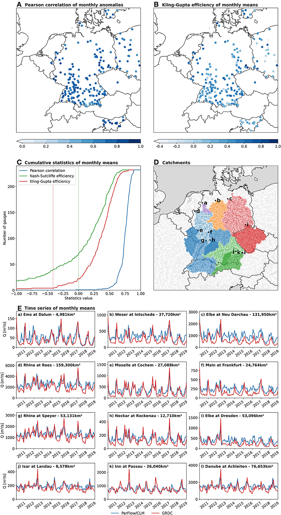
Figure 6. Comparison of the monthly discharge simulated by ParFlow/CLM and the observed GRDC discharge over 2011–2019. (A) Pearson correlation coefficient of the monthly mean discharge anomaly for all 231 grid cells corresponding to a GRDC gauge. The 222 grid cells with a significant correlation coefficient (p-value < 0.01) are depicted by big circles. (B) Kling–Gupta efficiency score (KGE) of the monthly mean discharge. (C) Cumulative distribution functions for the Pearson correlation coefficient (R), the Nash–Sutcliffe efficiency score (NSE), and the Kling–Gupta efficiency score (KGE) for the monthly mean discharge. The vertical dotted lines represent the mean flow benchmarks for NSE (0) and KGE (-0.41). (D) Catchments of the time series shown in (E). (E)(a)–(l) Time series of monthly mean discharge for 12 selected catchments marked on the map in (D).
5. Application examples
As explained above, DE06 is implemented in a prototypical monitoring and forecasting system focusing on the surface and subsurface water budget. It is deployed within the framework of the ADAPTER (ADAPt TERrestrial systems) project, funded by the Helmholtz Association of German Research Centres, which aims to develop simulation-based prototypical information products to support agriculture increasing its resilience against weather extremes and climate change in Germany. Thus, this monitoring and forecasting system aims to provide information on the evolution of the subsurface water budget that can be used for decision support. The diagnostics derived from the ParFlow/CLM simulations and described below have been widely developed in dialogue with stakeholders from the agricultural sector, such as farmers, chambers of agriculture, advisers, or plant breeders, in a so-called co-creation process. Nevertheless, as a multitude of diagnostics, indicators, and indices based on the subsurface water state and fluxes can be calculated from these simulations from the surface down to 60 m depth, this monitoring and forecasting system offers the opportunity to provide relevant information to a wide variety of users and stakeholders (e.g., related to forestry, ecosystem services, and especially water resources management).
From the ParFlow pressure fields and the soil hydraulic parameters, various indices and diagnostics describing different aspects of the subsurface water budget states and fluxes can be derived (Figure 7) at high spatial resolution for different depth layers. For example, the fraction of plant available water, which represents the soil water content scaled between the wilting point (0%) and the field capacity (100%), provides information on the water stress plants might suffer (Figure 7A). Another information on the subsurface water availability, and thus the water stress as well as the water resources, is provided by the subsurface water storage given, for example, as the anomaly of the current state compared to the reference time series over the last 11 years (Figure 7B). A third example is the vertical water flux, which allows the user to evaluate whether water is percolating, thus regenerating the subsurface water resources, but also whether nutrients might leach out of the root zone into the groundwater (Figure 7C). This kind of diagnostics can be calculated for every model grid layer, and thus the depth can be chosen to correspond, e.g., to the root depth of crops, vegetables, or trees. The daily forecasts of these diagnostics derived from the DE06 forecasting system are publicly available on the project's website (https://adapter-projekt.de/, in German) either as maps showing the deterministic forecast as shown in Figures 7A–C or as time series as shown on Figure 7D. Analogously to meteograms for weather monitoring and forecasting, the time series provide the users with the evolution of diagnostics of the terrestrial water cycle at their location (here, aggregated on a 3 × 3 km2 grid). The time series allows for a representation of the deterministic forecast but also of the 50-member ensemble forecast to give information on the impact of the uncertainty of the weather forecast used as forcing on the subsurface water state and fluxes.
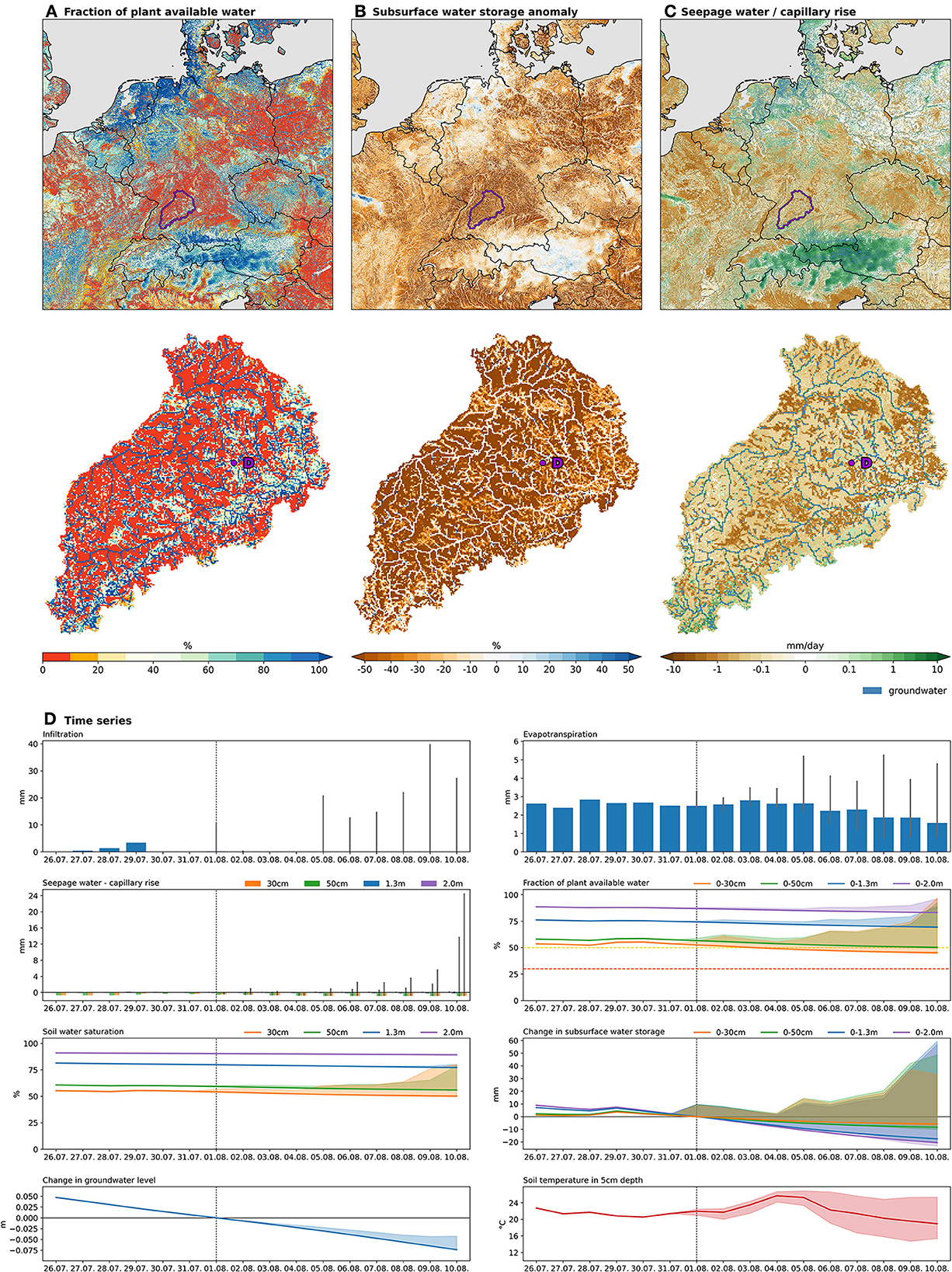
Figure 7. Examples of diagnostics derived from the forecast by the DE06 ParFlow/CLM simulation initialized at 2022-08-01T12:00Z. The maps show the deterministic forecast forced by ECMWF HRES for 2022-08-06T12:00Z (h + 120) for the entire DE06 domain extent and the Neckar catchment at Rockenau. (A) Fraction of plant available water (in %) from surface to 50 cm depth. (B) Subsurface water storage anomaly (in %) over the layer from the surface to 50 cm depth compared to the 31-day long-term mean over 2011–2021 centered on 01 August 2022. (C) Vertical water flow (in mm/day) at 50 cm depth (positive = downward). (D) Time series of daily values for one aggregated 3 × 3 km2 grid tile (i.e., 5x5 grid cells) selected as an example (see location in the Neckar catchment above). The solid lines (resp. bars) show the deterministic forecast, forced by ECMWF HRES, at the indicated depths or over the indicated thickness layers. The ensemble spread (min-max) of the 50-member ensemble forced by ECMWF ENS is shown as a shaded interval around the solid line or a gray vertical line over the bars, respectively. The vertical dotted line indicates the initialization of the forecast (here, 01 August 2022, 12 UTC). Data before initialization are taken from previous consecutive 24 h reference simulations forced by ECMWF HRES.
6. Summary and conclusion
In this study, we have introduced a new simulation setup (DE06) at high-resolution (0.611 km) encompassing some of the major central European river basins, that simulates surface and subsurface hydrodynamics and water budgets with the integrated hydrological model ParFlow/CLM aiming to provide users with relevant information on different components of the subsurface water budget at impact-relevant spatial and temporal scales. As the complete subsurface water budget is calculated over a 3D grid from the surface to 60 m depth for variably saturated conditions, all states and fluxes describing different aspects of the surface and subsurface water cycle can be derived from DE06. Here, we have outlined a monitoring and forecasting system, based on DE06 and forced by weather forecasts from ECMWF, that aims to provide various diagnostics that are meant to support the agricultural sector, but also other sectors that require knowledge about subsurface water resources, in their decision-making. Based on the GPU capability of ParFlow, enabling highly efficient simulations, the forecasting system includes a 50-member ensemble that allows an estimation of the impact of the uncertainty of the atmospheric forcing on the subsurface water budget.
The validation of the simulated reference time series with observation-based data over 2011–2020 shows a good agreement, especially concerning temporal dynamics. The good results obtained for the comparison of absolute monthly mean discharge values indicate that, even without calibration, DE06 can reproduce the observed surface and subsurface water cycle. This is further confirmed by the good agreement between simulation and observations for volumetric soil moisture, evapotranspiration, and water table depth, based on monthly mean anomalies.
In addition to the deterministic and ensemble forecasts over the next 10 days, we are expanding the monitoring and forecasting system with probabilistic seasonal ensemble predictions driven by the seasonal 50-member ensemble weather forecast SEAS from ECMWF. From these predictions, probabilities and risk assessments about the expected evolution of subsurface water resources and their impacts, e.g., recovery of the subsurface water storage after a drought, water stress for plants, and other stakeholder-relevant diagnostics, can be derived.
Further analyses may include, for example, a comparison of the obtained subsurface water budget time series when forcing DE06 with different atmospheric data sets, e.g., ERA5 reanalysis from ECMWF, and in particular different precipitation products, e.g., radar or satellite-based precipitation retrievals. A reanalysis-driven DE06 time series covering more than one decade would open the opportunity to study the evolution of the subsurface water budget over a longer period and to put in perspective the recent extreme hydrometeorological events, especially the droughts from 2018, 2019, 2020, and 2022.
The simulation setup presented in this study might further be improved, for example, by avoiding simplifying the fields defining the soil hydraulic properties (i.e., saturated hydraulic conductivity, porosity, and van Genuchten parameters), by using the USDA texture classes. Instead, the soil hydraulic properties could be determined for each grid cell with pedotransfer functions relying on the soil texture as given by SoilGrids, or even by using more complex pedotransfer functions, which also integrate, e.g., the bulk density and/or the soil organic carbon content. Another improvement could be achieved by an external coupling of ParFlow with a more complex land surface model that could, e.g., account for more land cover and crop types, calculate the carbon and nitrogen cycles, or offer the opportunity to assimilate satellite-based LAI (leaf area index) data to enhance the representation of the vegetation cycle. For the reference time series, long-term and interannual land cover changes could also be taken into account. A last improvement we want to emphasize would be the integration of the human impact on the subsurface water budget into DE06. This would cover a wide range of features and processes, such as drainage networks, groundwater pumping, or irrigation. Nevertheless, while ParFlow can account for these processes, it might be very difficult to implement them in the monitoring and forecasting system, especially over such a large domain, as this would require near-real-time information on, e.g., where, when, and how much water has been extracted from the system through pumping or added to it via irrigation.
Finally, since ParFlow/CLM is physics-based and does not rely on a calibration, which would make its parametrization climate-dependent, DE06 is also well-suited for climate change impact studies using future projections from, e.g., a global climate model or a regional climate model at high resolution. In this context, the CORDEX-compatible grid used in DE06 facilitates its integration into a fully coupled terrestrial model system at a convection-permitting scale, hence accounting for the feedback of the subsurface water budget on the atmosphere, making it suitable for impact studies both for recent and future climate conditions. In addition, as it relies almost entirely on global data sets (e.g., SoilGrids for soil texture) and globally defined parameters (e.g., USDA soil texture classification, IGBP land cover types), the workflow, with which DE06 has been built, can be easily expanded to the whole European continent or transferred to any region on the globe, including sparsely gauged regions, as it does not require calibration.
Data availability statement
The raw data supporting the conclusions of this article will be made available by the authors, without undue reservation.
Author contributions
AB co-designed and implemented the model setup and the monitoring and forecasting system and conducted all simulations, produced all figures, and carried out the writing of the original manuscript and its revision. KG and SK were involved in the and supported the implementation of the model setup and the monitoring and forecasting system and helped develop the analysis tools. KG, SK, JE, DR, and JV acquired the project funding. All authors supported the design of the application example (application of the monitoring and forecasting system for agricultural needs) and participated in the analysis and discussions of the results and the revision of the manuscript. All authors contributed to the article and approved the submitted version.
Funding
We acknowledge funding from the Impulse and Networking Fund of the Helmholtz Association of German Research Centres for the project ADAPTER (Adapt Terrestrial Systems; funding reference WT-0104). Additionally, this study was supported by funds of the BMBF BioökonomieREVIER funding scheme with its BioRevierPlus project (funding reference 031B1137D/031B1137DX). Furthermore, we gratefully acknowledge the Earth System Modelling Project (ESM) for funding this study by providing computing time on the ESM partition of the supercomputer JUWELS at Jülich Supercomputing Centre (JSC).
Acknowledgments
We thank the ECMWF for providing access to their weather forecast data. We also want to thank the authors of the different data sets DE06 is based on or that have been used for its validation, i.e., SoilGrids250m, IHME, ASTER, MERIT, CLC2018, CLM, ESA CCI, GLEAM, and GRDC, for making their data publicly available. The Climate Limited-area Modelling Community (CLM-Community) is thanked for providing access to the EXTPAR tool via the webPEP interface. Finally, we want to thank Yueling Ma for processing the water table depth observation data she collected for her doctoral thesis onto the DE-0055 grid for the validation of DE06.
Conflict of interest
The authors declare that the research was conducted in the absence of any commercial or financial relationships that could be construed as a potential conflict of interest.
Publisher's note
All claims expressed in this article are solely those of the authors and do not necessarily represent those of their affiliated organizations, or those of the publisher, the editors and the reviewers. Any product that may be evaluated in this article, or claim that may be made by its manufacturer, is not guaranteed or endorsed by the publisher.
Abbreviations
ADAPTER, ADAPt TERrestrial systems; ASTER, Advanced Spaceborne Thermal Emission and Reflection Radiometer; CDO, Climate Data Operators; CLC, Corine Land Cover; CLM, Common Land Model; CLM-Community, Climate Limited-area Modeling Community; CORDEX, COordinated Regional Downscaling EXperiment; DE-0055, DE06 grid at 0.0055° resolution (in rotated coordinates); DE06, ParFlow/CLM simulation setup at 0.6 km resolution over Germany and surrounding regions; DEM, Digital Elevation Model; ECMWF, European Centre; ENS, 50-member ensemble 10-day forecast from ECMWF; ERA5, Fifth generation ECMWF atmospheric reanalysis; ESA CCI, European Space Agency Climate Change Initiative; ET, Evapotranspiration; EUR-11, Pan-European CORDEX grid at 11 km resolution; EXTPAR, External Parameter for Numerical Weather Prediction and Climate Application; GDEM, Global Digital Elevation Model; GLEAM, Global Land Evaporation Amsterdam Model; GPU, Graphics Processing Unit; GRDC, Global Runoff Data Centre; HPC, High Performance Computing; HRES, High resolution deterministic 10-day forecast from ECMWF; IGBP, International Geosphere-Biosphere Programme; IHM, Integrated Hydrological Model; IHME, International Hydrogeological Map of Europe; JSC, Jülich Supercomputing Centre; KGE, Kling-Gupta efficiency score; LAI, Leaf Area Index; LSM, Land Surface Model; MERIT DEM, Multi-Error-Removed Improved-Terrain DEM; NSE, Nash-Sutcliffe efficiency score; PDE, Partial Differential Equations; PFT, Plant Functional Type; Q, Discharge; RMSE, Root-mean-square error; SEAS, 50-member seasonal 7-month forecast from ECMWF; TSMP, Terrestrial Systems Modelling Platform; USDA, United States Department of Agriculture; volSM, volumetric Soil Moisture; WTD, Water Table Depth.
References
Abrams, M., Crippen, R., and Fujisada, H. (2020). ASTER global digital elevation model (GDEM) and ASTER global water body dataset (ASTWBD). Remote Sens. 12, 1156. doi: 10.3390/rs12071156
Babaeian, E., Sadeghi, M., Jones, S., Montzka, C., Vereecken, H., and Tuller, M. (2019). Ground, proximal, and satellite remote sensing of soil moisture. Rev. Geophys. 57, 530–616. doi: 10.1029/2018RG000618
Boergens, E., Güntner, A., Dobslaw, H., and Dahle, C. (2020). Quantifying the central European droughts in 2018 and 2019 with GRACE Follow-On. Geophys. Res. Lett. 47, e2020GL087285. doi: 10.1029/2020GL087285
Bogner, K., Liechti, K., Bernhard, L., Monhart, S., and Zappa, M. (2018). Skill of hydrological extended range forecasts for water resources management in Switzerland. Water Resour. Manag. 32, 969–984. doi: 10.1007/s11269-017-1849-5
Bolton, D. (1980). The computation of equivalent potential temperature. Monthly Weather Rev. 108, 1046–1053. doi: 10.1175/1520-0493(1980)108<1046:TCOEPT>2.0.CO2
Brás, T., Seixas, J., Carvalhais, N., and Jägermeyr, J. (2021). Severity of drought and heatwave crop losses tripled over the last five decades in Europe. Environ. Res. Lett. 16, 065012. doi: 10.1088/1748-9326/abf004
Ciais, P., Reichstein, M., Viovy, N., Granier, A., Ogée, J., Allard, V., et al. (2005). Europe-wide reduction in primary productivity caused by the heat and drought in 2003. Nature 437, 529–533. doi: 10.1038/nature03972
Corine Land Cover (2018). Copernicus Land Monitoring Service (2020). Available online at: https://land.copernicus.eu/pan-european/corine-land-cover/clc2018 (accessed March 12, 2020).
Dai, Y., Zeng, X., Dickinson, R. E., Baker, I., Bonan, G. B., Bosilovich, M. G., et al. (2003). The common land model. B. Am. Meteorol. Soc., 84, 1013–1023. doi: 10.1175/BAMS-84-8-1013
Dasgupta, A., Arnal, L., Emerton, R., Harrigan, S., Matthews, G., Muhammad, A., et al. (2023). Connecting hydrological modelling and forecasting from global to local scales: perspectives from an international joint virtual workshop. J. Flood Risk Manag. in press. doi: 10.1111/jfr3.12880
Dorigo, W., Gruber, A., De Jeu, R., Wagner, W., Stacke, T., Loew, A., et al. (2015). Evaluation of the ESA CCI soil moisture product using ground-based observations. Remote Sens. Environ. 162, 380–395. doi: 10.1016/j.rse.2014.07.023
Dorigo, W., Wagner, W., Albergel, C., Albrecht, F., Balsamo, G., Brocca, L., et al. (2017). ESA CCI Soil Moisture for improved Earth system understanding: State-of-the art and future directions. Remote Sens. Environ. 203, 185–215. doi: 10.1016/j.rse.2017.07.001
Duscher, K., Günther, A., Richts, A., Clos, P., Philipp, U., and Struckmeier, W. (2015). The GIS layers of the “International Hydrogeological Map of Europe 1:1,500,000” in a vector format. Hydrogeol. J. 23, 1867–1875. doi: 10.1007/s10040-015-1296-4
Fang, Z., Bogena, H., Kollet, S., Koch, J., and Vereecken, H. (2015). Spatio-temporal validation of long-term 3D hydrological simulations of a forested catchment using empirical orthogonal functions and wavelet coherence analysis. J. Hydrol. 529, 1754–1767. doi: 10.1016/j.jhydrol.2015.08.011
Frei, S., Fleckenstein, J. H., Kollet, S. J., and Maxwell, R. M. (2009). Patterns and dynamics of river-aquifer exchange with variably-saturated flow using a fully-coupled model. J. Hydrol. 375, 383–393. doi: 10.1016/j.jhydrol.2009.06.038
Furusho-Percot, C., Goergen, K., Hartick, C., Kulkarni, K., Keune, J., and Kollet, S. (2019). Pan-European groundwater to atmosphere terrestrial systems climatology from a physically consistent simulation. Sci. Data 6, 320. doi: 10.1038/s41597-019-0328-7
Furusho-Percot, C., Goergen, K., Hartick, C., Poshyvailo-Strube, L., and Kollet, S. (2022). Groundwater model impacts multiannual simulations of heat waves. Geophys. Res. Lett. 49, e2021GL096781. doi: 10.1029/2021GL096781
Grillakis, M. (2019). Increase in severe and extreme soil moisture droughts for Europe under climate change. Sci. Total Environ. 660, 1245–1255. doi: 10.1016/j.scitotenv.2019.01.001
Gruber, A., De Lannoy, G., Albergel, C., Al-Yaari, A., Brocca, L., Calvet, J.-C., et al. (2020). Validation practices for satellite soil moisture retrievals: what are (the) errors? Remote Sens. Environ. 244, 111806. doi: 10.1016/j.rse.2020.111806
Gruber, A., Scanlon, T., van der Schalie, R., Wagner, W., and Dorigo, W. (2019). Evolution of the ESA CCI Soil Moisture climate data records and their underlying merging methodology. Earth Syst. Sci. Data 11, 717–739. doi: 10.5194/essd-11-717-2019
Gutowski, W., Giorgi, F., Timbal, B., Frigon, A., Jacob, D., Kang, H.-S., et al. (2016). WCRP COordinated Regional Downscaling EXperiment (CORDEX): a diagnostic MIP for CMIP6. Geosci. Model Dev. 9, 4087–4095. doi: 10.5194/gmd-9-4087-2016
Hari, V., Rakovec, O., Markonis, Y., Hanel, M., and Kumar, R. (2020). Increased future occurrences of the exceptional 2018-2019 central European drought under global warming. Sci. Rep. 10, 12207, doi: 10.1038/s41598-020-68872-9
Hartick, C., Furusho-Percot, C., Goergen, K., and Kollet, S. (2021). An interannual probabilistic assessment of subsurface water storage over Europe using a fully coupled terrestrial model. Water Resour. Res. 57, e2020WR027828. doi: 10.1029/2020WR027828
Hengl, T., Mendes de Jesus, J., Heuvelink, G. B. M., Ruiperez Gonzalez, M., Kilibarda, M., Blagotić, A., et al. (2017). SoilGrids250m: global gridded soil information based on machine learning. PLoS ONE 12, e0169748. doi: 10.1371/journal.pone.0169748
Hokkanen, J., Kollet, S., Kraus, J., Herten, A., Hrywniak, M., and Pleiter, D. (2021). Leveraging HPC accelerator architectures with modern techniques – hydrologic modeling on GPUs with ParFlow. Comput. Geosci. 25, 1579–1590. doi: 10.1007/s10596-021-10051-4
Ionita, M., Nagavciuc, V., Kumar, R., and Rakovec, O. (2020). On the curious case of the recent decade, mid-spring precipitation deficit in central Europe. npj Clim. Atmos. Sci. 3, 49. doi: 10.1038/s41612-020-00153-8
Keune, J., Gasper, F., Goergen, K., Hense, A., Shrestha, P., Sulis, M., et al. (2016). Studying the influence of groundwater representations on land surface-atmosphere feedbacks during the European heat wave in 2003. J. Geophys. Res. Atmos. 121, 13301–13325. doi: 10.1002/2016JD025426
Keune, J., Sulis, M., Kollet, S., Siebert, S., and Wada, Y. (2018). Human water use impacts on the strength of the continental sink for atmospheric water. Geophys. Res. Lett. 45, 4068–4076. doi: 10.1029/2018GL077621
Klages, S., Heidecke, C., and Osterburg, B. (2020). The impact of agricultural production and policy on water quality during the dry year 2018, a case study from Germany. Water 12, 1519. doi: 10.3390/w12061519
Knoben, W., Freer, J., and Woods, R. (2019). Technical note: inherent benchmark or not? Comparing Nash-Sutcliffe and Kling-Gupta efficiency scores. Hydrol. Earth Syst. Sci. 23, 4323–4331. doi: 10.5194/hess-23-4323-2019
Knoll, L., Häußermann, U., Breuer, L., and Bach, M. (2020). Spatial distribution of integrated nitrate reduction across the unsaturated zone and the groundwater body in Germany. Water 12, 2456. doi: 10.3390/w12092456
Koch, J., Cornelissen, T., Fang, Z., Bogena, H., Diekkrüger, B., Kollet, S., et al. (2016). Inter-comparison of three distributed hydrological models with respect to seasonal variability of soil moisture patterns at a small forested catchment. J. Hydrol. 533, 234–249. doi: 10.1016/j.jhydrol.2015.12.002
Kollet, S. J. (2009). Influence of soil heterogeneity on evapotranspiration under shallow water table conditions: transient, stochastic simulations. Environ. Res. Lett. 4, 035007. doi: 10.1088/1748-9326/4/3/035007
Kollet, S. J., Gasper, F., Brdar, S., Goergen, K., Hendricks-Franssen, H.-J., Keune, J., et al. (2018). Introduction of an experimental terrestrial forecasting/monitoring system at regional to continental scales based on the Terrestrial Systems Modeling Platform (v1.1.0). Water 10, 1–17. doi: 10.3390/w10111697
Kollet, S. J., and Maxwell, R. M. (2006). Integrated surface-groundwater flow modeling: a free-surface overland flow boundary condition in a parallel groundwater flow model. Adv. Water Resour. 29, 945–958. doi: 10.1016/j.advwatres.2005.08.006
Kuffour, B. N. O., Engdahl, N. B., Woodward, C. S., Condon, L. E., Kollet, S., and Maxwell, R. M. (2020). Simulating coupled surface-subsurface flows with ParFlow v3.5.0: capabilities, applications, and ongoing development of an open-source, massively parallel, integrated hydrologic model. Geosci. Model Dev. 13, 1373–1397. doi: 10.5194/gmd-13-1373-2020
Lehner, B., Verdin, K., and Jarvis, A. (2008). New global hydrography derived from spaceborne elevation data. Eos Transactions AGU 89, 93–94. doi: 10.1029/2008EO100001
Lehner, F., Coats, S., Stocker, T., Pendergrass, A., Sanderson, B., Raible, C., et al. (2017). Projected drought risk in 1.5°C and 2°C warmer climates. Geophys. Res. Lett. 44, 7419–7428. doi: 10.1002/2017GL074117
Ma, Y., Montzka, C., Naz, B., and Kollet, S. (2022). Advancing AI-based pan-European groundwater monitoring. Environ. Res. Lett. 17, 114037. doi: 10.1088/1748-9326/ac9c1e
Maina, F., Siirila-Woodburn, E., and Vahmani, P. (2020). Sensitivity of meteorological-forcing resolution on hydrologic variables. Hydrol. Earth Syst. Sci. 24, 3451–3474. doi: 10.5194/hess-24-3451-2020
Martens, B., Miralles, D. G., Lievens, H., van der Schalie, R., de Jeu, R. A. M., Fernández-Prieto, D., et al. (2017). GLEAM v3: satellite-based land evaporation and root-zone soil moisture. Geosci. Model Dev. 10, 1903–1925. doi: 10.5194/gmd-10-1903-2017
Maxwell, R. M., Condon, L. E., and Kollet, S. J. (2015). A high-resolution simulation of groundwater and surface water over most of the continental US with the integrated hydrologic model ParFlow v3. Geosc. Model Dev. 8, 923–937. doi: 10.5194/gmd-8-923-2015
Maxwell, R. M., and Kollet, S. J. (2008a). Quantifying the effects of three-dimensional subsurface heterogeneity on Hortonian runoff processes using a coupled numerical, stochastic approach. Adv. Water Resour. 31, 807–817. doi: 10.1016/j.advwatres.2008.01.020
Maxwell, R. M., and Kollet, S. J. (2008b). The interdependence of groundwater dynamics and land-energy feedbacks under climate change. Nat. Geosci. 1, 665–669. doi: 10.1038/ngeo315
Maxwell, R. M., Kollet, S. J., Smith, S. G., Woodward, C. S., Falgout, R. D., Ferguson, I. M., et al. (2016). ParFlow User's Manual. Integrated GroundWater Modeling Center Report GWMI, 167p.
Maxwell, R. M., Putti, M., Meyerhoff, S. B., Delfs, J.-O., Ferguson, I. M., Ivanov, V., et al. (2014). Surface-subsurface model intercomparison: a first set of benchmark results to diagnose integrated hydrology and feedbacks. Water Resour. Res. 50, 1531–1549. doi: 10.1002/2013WR013725
Miralles, D. G., Holmes, T. R. H., De Jeu, R. A. M., Gash, J. H., Meesters, A. G. C. A., and Dolman, A. J. (2011). Global land-surface evaporation estimated from satellite-based observations. Hydrol. Earth Syst. Sci. 15, 453–469. doi: 10.5194/hess-15-453-2011
Moravec, V., Markonis, Y., Rakovec, O., Svoboda, M., Trnka, M., Kumar, R., et al. (2021). Europe under multi-year droughts: how severe was the 2014-2018 drought period? Environ. Res. Lett. 16, 034062. doi: 10.1088/1748-9326/abe828
Naumann, G., Cammalleri, C., Mentaschi, L., and Feyen, L. (2021). Increased economic drought impacts in Europe with anthropogenic warming. Nat. Clim. Chang. 11, 485–491. doi: 10.1038/s41558-021-01044-3
O'Neill, M., Tijerina, D., Condon, L., and Maxwell, R. (2021). Assessment of the ParFlow-CLM CONUS 1.0 integrated hydrologic model: evaluation of hyper-resolution water balance components across the contiguous United States. Geosci. Model Dev. 14, 7223–7254. doi: 10.5194/gmd-14-7223-2021
Orth, R., and Seneviratne, S. (2013). Predictability of soil moisture and stream?ow on subseasonal timescales: a case study. J. Geophys. Res. Atmos. 118, 10963–10979. doi: 10.1002/jgrd.50846
Owens, R. G., and Hewson, T. (2018). ECMWF Forecast User Guide. ECMWF, Reading. doi: 10.21957/m1cs7h. Available online at: https://www.ecmwf.int/node/16559
Penland, C., Fowler, M., Jackson, D., and Cifelli, R. (2021). Forecasts of opportunity for northern California soil moisture. Land 10, 713. doi: 10.3390/land10070713
Poméon, T., Wagner, N., Furusho, C., Kollet, S., and Reinoso-Rondinel, R. (2020). Performance of a PDE-based hydrologic model in a flash flood modeling framework in sparsely-gauged catchments. Water 12, 2157. doi: 10.3390/w12082157
Pylianidis, C., Osinga, S., and Athanasiadis, I. (2021). Introducing digital twins to agriculture. Comput. Electron. Agric. 184, 105942. doi: 10.1016/j.compag.2020.105942
Rahman, M., Sulis, M., and Kollet, S. J. (2014). The concept of dual-boundary forcing in land surface-subsurface interactions of the terrestrial hydrologic and energy cycles. Water Resour. Res. 50, 8531–8548. doi: 10.1002/2014WR015738
Reinermann, S., Gessner, U., Asam, S., Kuenzer, C., and Dech, S. (2019). The effect of droughts on vegetation condition in Germany: an analysis based on two decades of satellite Earth observation time series and crop yield statistics. Remote Sens. 11, 1783. doi: 10.3390/rs11151783
Rosenzweig, C., Iglesias, A., Yang, X., Epstein, P., and Chivian, E. (2001). Climate change and extreme weather events; Implications for food production, plant diseases, and pests. Glob. Change Hum. Health 2, 90–104. doi: 10.1023/A:1015086831467
Saadi, M., Furusho-Percot, C., Belleflamme, A., Chen, J.-Y., Trömel, S., and Kollet, S. (2023a). How uncertain are precipitation and peak flow estimates for the July 2021 flooding event? Nat. Hazards Earth Syst. Sci. 23, 159–177. doi: 10.5194/nhess-23-159-2023
Saadi, M., Furusho-Percot, C., Belleflamme, A., Trömel, S., Kollet, S., and Reinoso-Rondinel, R. (2023b). Comparison of three radar-based precipitation nowcasts for the extreme July 2021 flooding event in Germany. J. Hydrometeorol. doi: 10.1175/JHM-D-22-0121.1
Samaniego, L., Thober, S., Kumar, R., Wanders, N., Rakovec, O., Pan, M., et al. (2018). Anthropogenic warming exacerbates European soil moisture droughts. Nat. Clim. Change 8, 421–426. doi: 10.1038/s41558-018-0138-5
Samaniego, L., Thober, S., Wanders, N., Pan, M., Rakovec, O., Sheffield, J., et al. (2019). Hydrological forecasts and projections for improved decision-making in the water sector in Europe. Bull. Am. Meteorol. Soc. 100, 2451–2472. doi: 10.1175/BAMS-D-17-0274.1
Schalge, B., Haefliger, V., Kollet, S., and Simmer, C. (2019). Improvement of surface run-off in the hydrological model ParFlow by a scale-consistent river parameterization. Hydrol. Process. 33, 2006–2019. doi: 10.1002/hyp.13448
Schreiner-McGraw, A., and Ajami, H. (2020). Impact of uncertainty in precipitation forcing data sets on the hydrologic budget of an integrated hydrologic model in mountainous terrain. Water Resour. Res. 56, e2020WR027639. doi: 10.1029/2020WR027639
Schulzweida, U. (2021). CDO User Guide (Version 2.0.0). Max-Planck-Institute for Meteorology, Hamburg: Zenodo. doi: 10.5281/zenodo.5614769
Shrestha, P. (2019). TerrSysMP Pre-processing and Post-processing System. CRC/TR32 Database (TR32DB). doi: 10.5880/TR32DB.37 Available online at: https://www.tr32db.uni-koeln.de/search/view.php?doiID=111 (accessed April 2, 2020).
Singla, S., Céron, J.-P., Martin, E., Regimbeau, F., Déqué, M., Habets, F., et al. (2012). Predictability of soil moisture and river flows over France for the spring season. Hydrol. Earth Syst. Sci. 16, 201–216. doi: 10.5194/hess-16-201-2012
Spinoni, J., Barbosa, P., Bucchignani, E., Cassano, J., Cavazos, T., Christensen, J., et al. (2020). Future global meteorological drought hot spots: a study based on CORDEX data. J. Clim. 33, 3635–3661. doi: 10.1175/JCLI-D-19-0084.1
Thober, S., Kumar, R., Sheffield, J., Mai, J., Schäfer, D., and Samaniego, L. (2015). Seasonal soil moisture drought prediction over Europe using the North American Multi-Model Ensemble (NMME). J. Hydrometeorol. 16, 2329–2344. doi: 10.1175/JHM-D-15-0053.1
Trnka, M., Hlavinka, P., MoŽný, M., Semerádová, D., Štěpánek, P., Balek, J., et al. (2020). Czech Drought Monitor System for monitoring and forecasting agricultural drought and drought impacts. Int. J. Climatol. 40, 5941–5958. doi: 10.1002/joc.6557
Van Genuchten, M. T. (1980). A closed-form equation for predicting the hydraulic conductivity of unsaturated soils. Soil Sci. Soc. Am. J., 44, 892–898. doi: 10.2136/sssaj1980.03615995004400050002x
Wanders, N., Thober, S., Kumar, R., Pan, M., Sheffield, J., Samaniego, L., et al. (2019). Development and evaluation of a pan-European multimodel seasonal hydrological forecasting system. J. Hydrometeorol. 20, 99–115. doi: 10.1175/JHM-D-18-0040.1
Wendland, F., Bergmann, S., Eisele, M., Gömann, H., Herrmann, F., Kreins, P., et al. (2020). Model-based analysis of nitrate concentration in the leachate – the North Rhine-Westfalia case study, Germany. Water 12, 550. doi: 10.3390/w12020550
Yamazaki, D., Ikeshima, D., Sosa, J., Bates, P. D., Allen, G. H., and Pavelsky, T. M. (2019). MERIT hydro: a high-resolution global hydrography map based on latest topography datasets. Water Resour. Res. 55, 5053–5073. doi: 10.1029/2019WR024873
Zappa, M., Bernhard, L., Spirig, C., Pfaundler, M., Stahl, K., Kruse, S., et al. (2014). A prototype platform for water resources monitoring and early recognition of critical droughts in Switzerland. Proc. IAHS 364, 492–498. doi: 10.5194/piahs-364-492-2014
Zhang, Y., and Schaap, M. (2017). Weighted recalibration of the Rosetta pedotransfer model with improved estimates of hydraulic parameter distributions and summary statistics (Rosetta3). J. Hydrol. 547, 39–53. doi: 10.1016/j.jhydrol.2017.01.004
Zhu, L., Wang, H., Tong, C., Liu, W., and Du, B. (2019). Evaluation of ESA active, passive and combined soil moisture products using upscaled ground measurements. Sensors 19, 2718. doi: 10.3390/s19122718
Keywords: monitoring and forecasting, stakeholder relevant scales, ParFlow/CLM hydrological model, high-resolution hydrological modeling, subsurface water resources, terrestrial water budget, applied information, computing on GPUs
Citation: Belleflamme A, Goergen K, Wagner N, Kollet S, Bathiany S, El Zohbi J, Rechid D, Vanderborght J and Vereecken H (2023) Hydrological forecasting at impact scale: the integrated ParFlow hydrological model at 0.6 km for climate resilient water resource management over Germany. Front. Water 5:1183642. doi: 10.3389/frwa.2023.1183642
Received: 10 March 2023; Accepted: 08 May 2023;
Published: 30 May 2023.
Edited by:
Osayed S. M. Abu-Elyazeed, Helwan University, EgyptReviewed by:
Tamer A. Elbana, National Research Centre, EgyptMichele Vurro, National Research Council (CNR), Italy
Copyright © 2023 Belleflamme, Goergen, Wagner, Kollet, Bathiany, El Zohbi, Rechid, Vanderborght and Vereecken. This is an open-access article distributed under the terms of the Creative Commons Attribution License (CC BY). The use, distribution or reproduction in other forums is permitted, provided the original author(s) and the copyright owner(s) are credited and that the original publication in this journal is cited, in accordance with accepted academic practice. No use, distribution or reproduction is permitted which does not comply with these terms.
*Correspondence: Alexandre Belleflamme, a.belleflamme@fz-juelich.de