Daily Subsurface Ocean Temperature Climatology Using Multiple Data Sources: New Methodology

1. Introduction

Over the next decades, ocean ecosystems and the networks that rely on them will come under increased pressure from a changing climate system. To sustain the future of our oceans, improving the availability and accessibility of oceanographic data is required, and should be aimed at both the ocean research community and recognized stakeholders, such as fisheries, government, and businesses (Bailey et al., 2019; Benway et al., 2019; Buck et al., 2019; Iwamoto et al., 2019). Multi-decadal ocean temperature records provide context to recent warming, allow studies of physical processes on a range of timescales, and aid with model validation and forecasting. Australia is in the enviable position of having some of the longest subsurface oceanographic temperature records in the world. Seven National Reference Stations (NRS) are currently in operation, part of Australia's Integrated Marine Observing System (IMOS), with three stations having temperature records spanning more than 65 years (Thompson et al., 2009; Lynch et al., 2014). Designing data products that incorporate long temperature records, such as these, allow for easier dissemination and usability of data, helping to deliver on global goals and initiatives (e.g., Sustainable Development Goal SDG14 (Visbeck et al., 2014; Nations, 2015), and the United Nations Decade of Ocean Science for Sustainable Development (UNESCO, 2019).

A climatology describes the mean state of a variable. Such mean state is useful for relating long-term patterns with short term variability, allowing the identification of periods of anomalously high or low conditions (Schaeffer and Roughan, 2017; Schlegel et al., 2017; Oliver et al., 2018). Anomalously warm events, such as marine heatwaves (MHWs), are commonly defined as prolonged discrete events when temperatures are warmer than the 90th percentile (based on at least a 30 year long climatology) for 5 days or more (Hobday et al., 2016). Defining MHWs thus require daily climatologies, and enable us to monitor the health of an ecosystem, and to understand change in the marine environment (e.g., frequency and duration of anomalous periods).

Numerical ocean models, useful for assessing and understanding physical and biogeochemical changes, forecasting, and projecting future oceanic change, depend on observations to accurately simulate the marine environment (e.g., to better predict the timing and location of eddies). A comparison between the mean states of a model with that from a climatology provides an indication of how well a model performs (e.g., Kerry et al., 2016).

Climatology data products and their corresponding visualizations are powerful tools for ocean monitoring. The use of web-based apps to compare climatologies with real-time data, such as the IMOS OceanCurrent (http://oceancurrent.imos.org.au/) and the Northwest Association of Networked Ocean Observing Systems (NANOOS, http://nvs.nanoos.org/Climatology) web-apps, enable end-users to monitor the marine environment efficiently using an easily understandable format (Bailey et al., 2019). Developing methodologies to combine data records obtained from different platforms over varying timescales for use in climatology data products optimizes the utility of an observing system, enabling the monitoring and assessment of a marine environment, whilst providing access to data and information for end users.

Many global and regional ocean climatology data products are available. Globally popular climatology data products include the Global Ocean Data Analysis Project (GLODAP, Lauvset et al., 2016; Olsen et al., 2016), the World Ocean Atlas (WOA, Levitus, 1983; Locarnini et al., 2019), the World Ocean Circulation Experiment (WOCE) Global Hydrographic Climatology (Gouretski, 2018), and the Commonwealth Scientific and Industrial Research Organization (CSIRO) Atlas of Regional Seas (CARS, Ridgway et al., 2002). Global climatology products, such as these, typically provide objectively analyzed/mapped climatological fields or spatially-binned statistics (e.g., Sabine et al., 2013) for a range of vertical levels to account for the sparse spatial distribution of high quality data (e.g., GLODAP has 33 standard depth levels). Although useful for global studies, such climatology data products may not accurately represent intra-annual variability at some locations (particularly close to shore) related to data product resolution (e.g., CARS is 0.5 degrees), data distribution, and the choice of input data. For some global data products, the recent increase in data coverage has lead to some temporal biasing of the climatological statistics in some regions (e.g., CARS, Dunn, 2011). In Australasia, the Sea Surface Temperature (SST) Atlas of Australian Regional Seas (SSTAARS, Wijffels et al., 2018) daily climatology uses 25 years of Advanced Very High-Resolution Radiometer (AVHRR) data from NOAA Polar Orbiting Environmental Satellites to produce an SST climatology at a depth of approximately 20 cm. Although high-resolution (~ 2 km) mean variability is provided in time and horizontal space, this climatology data product uses just one data source as input and at the surface only.

There is demand to make climatology data products utilizing multiple data sets combining long ocean records available for end users (Bailey et al., 2019). Long ocean records capture seasonal variability over many years. These long-term intra-annual patterns are clear in daily climatologies, critical when dealing with parameters like ocean temperature. However, over time the availability of resources and the priorities of stakeholders change while research and technology advances lead to changes in best practices and instrumentation. As a consequence, long temperature records can consist of data with varying resolution in time and space, can often have gaps that last from a few weeks to years, and can contain data of varying quality.

This paper demonstrates a methodology to create a subsurface temperature climatology data product using data from the Port Hacking National Reference Station (NRS); this site is described in more detail in section 2. A 66 year long temperature record was used, consisting of bottle data collected typically every 1 to 4 weeks at discrete depths between 1953 and 2010, and from 2009 on near-monthly vertical profiling CTD profiles and 5 min moored data at discrete depths through the water column. Although a range of subsurface climatologies exist, some of the following statements can be true: (1) not all available data are used, (2) their resolution are sometimes too coarse, (3) their accuracy tend to decrease closer to the coast, and (4) bias relating to changes in recent data coverage is sometimes an issue.

The methodology described here combines three data sets of varying resolution at seven depths, taking into account the recent increase in spatial and temporal data coverage. Effort has been made to ensure the quality of the combined temperature data, and gaps have been filled within pre-determined spatial and temporal limits. The temperature data sources, quality control procedures, and the data processing steps used to create the climatology are described in sections 3 and 4.1. Intra-daily temperature variability is explored in section 4.2, and a unique validation technique using synthetically-created data is described in section 4.3. The resulting climatology data product (including the daily means, 10th and 90th percentiles), and the paper's conclusions are presented in sections 5 and 6, respectively.

2. The Study Region

The data used were collected at the Port Hacking historical sampling and mooring site (NRSPHB / PH100) at approximately 34° S, 6 km off the coast of the greater Sydney region. The site, which is in approximately 100 m of water (Figure 1A) was initially named Port Hacking station “B” (PHB), maintained through the CSIRO Coastal Monitoring Program, and most recently by the New South Wales (NSW) Office of Environment and Heritage (since mid 2019 the Department of Planning, Industry and Environment). In 2010, this site became recognized as one of nine (now seven) “National Reference Stations” (NRS) around Australia (Lynch et al., 2014) where sampling continues. At this time the site was renamed “NRSPHB.” The PH100 mooring was deployed in 2009 as part of the NSW-IMOS moorings programme (the New South Wales node of IMOS, www.imos.org.au), led by the University of New South Wales (UNSW) Sydney (Roughan and Morris, 2011; Roughan et al., 2013, 2015).

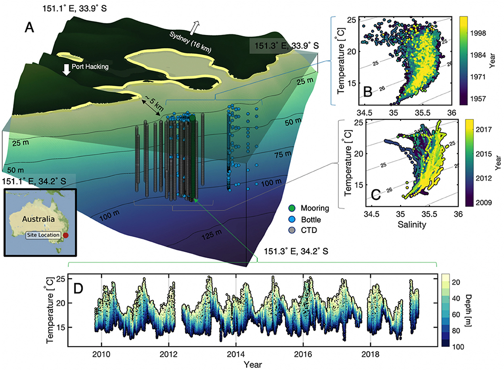
Figure 1. (A) A 3D representation of the Port Hacking study site alongside its location in Australia. The locations and depths of the chosen bottle samples, CTD profiles, and the PH100 mooring are displayed. The black labeled contour lines represent the bathymetry in the area. The bottle (B) and CTD profile (C) T-S diagrams are shown, colored by the year in which they were collected, superimposed over potential density anomaly contours. The PH100 mooring temperatures as a function of time are displayed (D), colored by the depth in which they were recorded.

3. Data Sources

The temperature climatology was produced using three near-surface to bottom seawater temperature data sources (Table 1). These are:

1. Bottle data: Data were obtained from approximately weekly to monthly bottle samples collected between 1953 and 2010 (presented by Schaeffer and Roughan, 2017 in Figure 1b). The depths of the bottle samples have varied over time, but the most consistent depths are 0, 10, 50, 75, and 100 m. The majority of bottles were collected in the morning (86%) local time (UTC+10), particularly between 09:00 and 11:00. Data were obtained using a deep-sea reversing thermometer attached to a sealing water sample bottle, and were corrected for thermal expansion (Fisheries, 1970). Data were sometimes replaced by temperature measured by the CTD. Between 2004 and 2010, reversing thermometers were used at just 2 depths (0 and 75 m). Temperature was measured by the CTD at the other remaining depths. The accuracy of this method was generally ±0.05°C in the 1940s (Rochford, 1951) but more recently could be as good as ±0.01°C when the instrument was properly calibrated (Abraham et al., 2013).

2. Mooring data: Moored time series data between 2009 and 2019 obtained at the PH100 (151.224 ° E, 34.119 ° S) mooring site (Figure 1D). The PH100 mooring was typically instrumented with a combination of 11 AQUATec Aqualogger 520T temperature or 520TP temperature and pressure sensors sampling at 5 min intervals at nominally 8 m vertical spacing from about 17 m below the surface to the bottom. Due to a dynamic and operationally-challenging surface environment (see Roughan et al., 2013) the PH100 mooring does not typically have a surface float (although a number of trials were conducted). Hence, moored surface observations were only available for a limited time, and were not considered here. Full details of the sustained mooring programme are described by Roughan et al. (2013). The temperature and pressure data have a nominal accuracy of ±0.05°C and 0.2%, respectively.

3. CTD data: Vertical profile data were obtained from shipboard conductivity, temperature and depth (CTD) sensor profiles (typically a SeaBird 19+ CTD) taken each time a boat visited the PH100 and NRSPHB sites (Figure 1C). The frequency of the data has been near-monthly since 2009. Similarly to the bottle data, the majority of the profiles were measured in the morning (98%) local time (UTC+10), particularly between 08:00 and 10:00 a.m. The temperature and depth data have a nominal accuracy of ±0.005°C and 0.1%, respectively.

Here on, the above-mentioned data are referred to as “bottle,” “mooring,” or “CTD” data for ease of reading. After collection, the data sources were quality controlled and processed, as described in section 4.1.1, before being uploaded to an online open access data portal. Each of the original data sources are freely available at www.aodn.org.au or http://www.marine.csiro.au/marlin/.

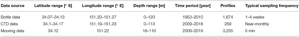
Table 1. Data description, including data source, location (latitude and longitude), depth range, time period, number of vertical profiles for each data type, and typical sampling frequency.

4. Materials and Methods

4.1. Data Processing Steps

4.1.1. Quality Assurance and Control

Temperature sensors used for mooring and CTD data were calibrated regularly (typically once per year) at a licensed calibration facility. A standardized IMOS data collection process was followed to ensure data is of high precision and accuracy. This process includes guidance on pre-deployment planning, data collection, post-deployment data processing, and quality control. It also includes instructions relating to sensor validation and maintenance, pre-run and post sensor checks and field sampling steps. More details about the procedures and the IMOS NRS network design and rationale are described by Sutherland et al. (2017) and Lynch et al. (2011), respectively.

IMOS quality control (QC) checks were applied to CTD and mooring data, which have been described in detail by Morello et al. (2014) and Ingleton et al. (2014). This included, but was not limited to, checking:

• The observation times for an impossible date

• Whether the observation was taken whilst the instrument was out of the water

• Whether the observation locations were outside of an expected range from the nominal latitude and longitude coordinates

• Whether the observation depths were within a realistic range

• Whether the parameter's values are within a global valid range

• Whether the parameter's values are within a regional valid range

• For a vertically adjacent triplet of observations (e.g., CTD data), whether a spike was present.

The QC'd data were processed through the IMOS data toolbox; a MATLAB software package designed to import, pre-process, and automatically/manually QC data (more information and scripts available from https://github.com/aodn/imos-toolbox/wiki). Afterwards, QC'd data were converted to Climate and Forecast compliant NetCDF files for archiving and dissemination. The data selected for the climatology computation were mooring and CTD data flagged as either “good data” or “probably good data” following UNESCO Intergovernmental Oceanographic Commission (IOC) protocol (flags 1 and 2, respectively) (Lynch et al., 2014; Morello et al., 2014), endorsed by Australia's IMOS programme.

For the bottle data, we included four additional QC steps. To limit the effect of erroneous temperatures on climatology statistics, an automatic outlier test was first applied. This QC test (Figure 2) flagged bottle temperatures outside of density-binned average temperatures ± three standard deviations using the entire bottle record (as used by Gouretski and Jancke, 1999). Any temperatures outside of these defined thresholds were considered as flagged outliers. Although it is believed that most extreme bottle temperatures were outliers resulting from the instrumentation used, a proportion of extreme temperatures that were flagged by this automatic outlier test could have been real, and hence may have been unnecessarily removed. However, due to the low quantity of extremes that were flagged in this way (<1%), there would be a limited effect on the climatology statistics. The second and third QC tests considered the location of the bottle data. In the second test, bottle data where the bottom depth of their corresponding cast was either shallower or deeper than the range of 80 to 120 m were flagged. The third test considered spatial separation. Bottle data considered too far away from the NRSPHB and PH100 sites were flagged. Maximum distance thresholds were defined using de-correlation scales of temperature spatial variability (37 km along-shelf and 14 km across-shelf) estimated by Schaeffer et al. (2016) using on-shelf glider measurements between 29.5 and 34°S in the top 50 m of the water column. The bottom depth second QC test flagged 9.8% of historical bottle samples, whereas the temperature de-correlation scale third QC test did not flag any additional samples. The locations of QC'd data are shown in Figure 1A. The fourth QC test identified bottle data where > 30 % of the samples within a selected vertical profile were flagged previously using the first three QC tests (e.g., erroneous profiles). No further bottle data were flagged by this fourth QC test. In total, 10.7 % of the bottle data were flagged when applying these four additional QC tests, with some samples flagged by more than one QC test.

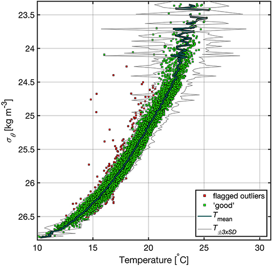
Figure 2. Automatic outlier test. Bottle sample temperatures outside of the mean ±3× standard deviation lower and upper thresholds (“flagged outliers”) determined using the entire bottle record are compared with temperature within the upper and lower thresholds (“good”). The density-binned mean profile (T_mean) and the ±3× density-binned standard deviation thresholds (T_±3xSD) are also shown.

All four QC tests described above were also applied to the CTD data, whilst only the two non-location-specific QC tests (first automatic outlier and fourth erroneous profile QC tests) were applied to the mooring data. As there are few density measurements at the PH100 mooring, the first automatic outlier QC test was initiated using depth bins instead of density bins. For each depth bin, temperatures outside of the depth-binned mean ± three standard deviations, calculated using the full mooring record, were flagged as outliers. A total of 1.3 and 12.3% of CTD and mooring data, respectively, were flagged via the IMOS standard automatic tests and the additional four bottle QC tests listed above. Although, almost all of these flagged CTD and mooring data were identified via the IMOS standard automatic QC tests.

4.1.2. Data Aggregation

The quality controlled data sets were aggregated as daily vertical “profiles.” For the bottle and CTD data, this is self explanatory as they were collected as profiles. Prior to aggregation, the 5 min interval mooring data were daily averaged and assigned regular daily timestamps. Close to a million moored measurements were used to create 3,235 daily profiles between approximately 16 and 100 m (Table 1). More than 1,600 bottle profiles and 259 CTD profiles were used alongside the mooring daily “profiles” to produce the daily climatology. The quality controlled bottle, CTD, and mooring temperature profiles were then combined into one file spanning 31 May 1953 to 31 May 2019 (66 years). For each day of the year, the data were collected over a number of years. Here, we refer to these as “binned years.” At this stage, there were on average 13.4 binned years available per day of the year.

4.1.3. Optimal Depths

To calculate a multiple depth climatology, we needed to bin the data into standard depths. Optimal climatology depth levels were chosen to maximize the number of binned years available. The daily climatology statistics were calculated at seven optimal depths: 19, 31, 41, 49, 74, 81, and 99 m, (shown in Figure 3) using data within 1 ± 2 m depth bin margins. These seven depths were determined using the 1 ± 2 m depth-binned vertical distributions of bottle and mooring data between the surface and 100 m depth from 1953 to 2019, normalized with respect to the depth bin containing the highest number of corresponding data source measurements. Depth bins that contained both bottle and mooring data were considered only. At some depths (e.g., 10 and 90 m) there were only bottle or mooring data, hence these depths were not considered. Optimal depths were determined where the depth-binned combined bottle and mooring normalized data sums (weighted 80% bottle data and 20% mooring data) was greater than a threshold of 0.5, chosen upon inspecting the weighted sums. As a final check, potential optimal depths were evaluated for the percentage of the year covered by, and the number of binned years present in, the available data within the chosen optimal 1 ± 2 m depth bin.

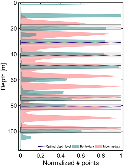
Figure 3. The total number of bottle and Mooring data points per 1 ± 2 m depth bin at the NRSPHB / PH100 site, normalized using the maximum number of data points available in a depth bin for the corresponding data source. This is accompanied by the chosen optimal depths with the corresponding depth bin margins (black rectangles).

4.1.4. Data Interpolation

As the Port Hacking site is dynamic, an auto-correlation analysis was performed using temperatures to estimate scales of variability in vertical space and time. The correlation of temperatures separated from one another by different time and distance lags was used to determine the potential limitations of interpolation in time and space at this site. The vertical spatial and temporal scales of variability were defined as the depth or time lag corresponding to a temperature correlation threshold of 0.7, as used by Schaeffer et al. (2013). This is in addition to the estimates by Roughan et al. (2013) and Roughan et al. (2015) using data from NSW-IMOS moorings off southeastern Australia. Vertically, the temperature auto-correlation threshold of 0.7 (using CTD data between 2009 and 2017) corresponded to depth separations of 8 to 9 m, dependent on season (Figure 4A). In time, the temperature coefficient threshold (using mooring data between 2013 and 2015) corresponded to time separations between 127 h (5.3 days) and 168 h (1 week), when comparing different depths (Figure 4B). These temporal scales of variability varied seasonally, with the temperature correlation thresholds ranging between a minimum of 59 h (2.5 days) at depths of 10–20 m in autumn when the water-column is typically stratified, and a maximum of 567 h (3.4 weeks) at depths of 35–45 m in Spring when the water-column is usually well-mixed.

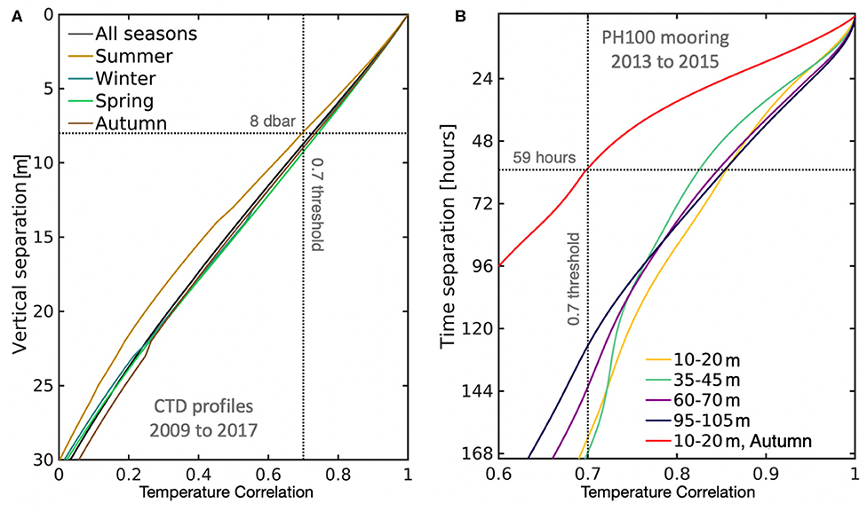
Figure 4. The autocorrelation function of temperature observations in vertical space and time. (A) The temperature correlation coefficients determined using ship CTD profiles between 2009 and 2017 as a function of vertical separation [m] for all seasons, summer (DJF), winter (JJA), spring (SON), and autumn (MAM). (B) The temperature correlation coefficients determined using PH100 mooring temperatures between 2013 and 2015 as a function of time separation (hours) between 10 and 20 m, 35 and 45 m, 60 and 70 m, and between 95 and 105 m for all seasons. The lowest correlation temporal threshold is plotted using data in Autumn between 10 and 20 m. Annotations are included in each sub panel describing the data that were used and the identified vertical and temporal correlation thresholds (labeled lines).

Linearly-interpolated temperatures were used to fill in vertical and temporal gaps in the record (shown in Figure 5). Gaps were filled vertically first, followed by gaps in time. The mean absolute difference was 0.04°C between the interpolated values used in this study and those resulting from temporal interpolation prior to spatial interpolation. Interpolated values greater than 8 m, and 2 days away from an observed sample were flagged and discarded from the climatology data product. After interpolation, the number of binned years per climatology day increased from 13.4 years to 28.6 years on average when considering all depths.

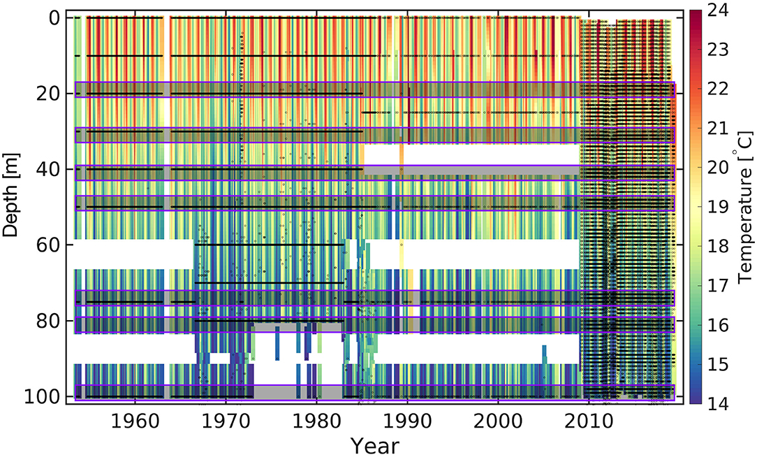
Figure 5. Interpolated daily temperatures with 1 m vertical spacing at the Port Hacking site between 1953 and 2019. The black circles represent the depths and times of non-interpolated temperature observations, whilst the transparent gray boxes with purple outlines represent the 1 ± 2 m depth bins used to produce the climatology.

4.1.5. Accounting for Data Source Sampling Characteristics

The interpolated aggregated temperature record contained daily mooring profiles, bottle profiles collected every 1 to 4 weeks, and CTD profiles collected typically near-monthly. As each data source contained in this aggregated record had a different method of retrieval, and therefore varying sampling characteristics, it was important to consider any related biasing of climatology statistics. The causes of potential bias were due to (1) most of the aggregated record consisting of mooring data, measured over the last decade which was warmer on average than other decades, (2) days of the year when limited bottle data were available potentially leading to warmer than expected statistics, and (3) dates when more than one data source was available. Methods have been established to partially counteract these bias, which are described below. Data organized into each of the time-depth bins used to calculate climatology statistics had a corresponding year and day of the year. In the text below, we refer to these as “binned years” (as mentioned previously) and “binned days.” Statistics are calculated for each day of the year, and hence will be referred to as “climatology days.”

On average 70% of the data available for a given climatology day was measured at the PH100 mooring between 2009 and 2019. The remaining 30% consisted of CTD data (19%) and bottle data (11%). The availability of data in each optimal depth bin and for each decade is shown in Figure 6. A significant long-term trend of approximately 1°C century⁻¹ at depths of 15–25 m was estimated at NRSPHB / PH100 using simple linear regression (see section 4.3.1 for more information relating to the methods of estimating this trend). This long-term trend estimate is higher than that estimated by Thompson et al. (2009) of approximately 0.75°C century⁻¹ using surface bottle data between 1953 and 2005 at NRSPHB, expected for a period that extends to 2019. As the mooring data, representing approximately 1 / 7 of the record, were warmer than the bottle data on average, the resulting climatology statistics would be biased.

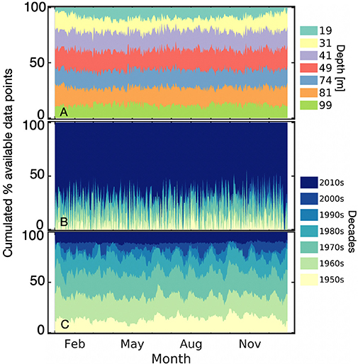
Figure 6. The cumulated percentage of (A) available data points used at each depth bin, (B) available data points for each decade, and (C) available data points for each decade when incorporating a ± 2 day time-centered window and a bottle to mooring (b:m) ratio of 6:1. Each panel shows the cumulated percentage for each climatology day.

To reduce the temperature bias of mooring data, the number of mooring binned years per climatology day was restricted. A bottle to mooring (b:m) binned year ratio of 6:1 was enforced for each climatology day, with the resulting proportions shown in Figure 6C: approximately 6 decades for bottle data (1953 to 2010), and approximately a decade for mooring data (2009 to 2019). The mooring binned years were selected at random from those available for the climatology day to match the necessary ratio. This reduced the mooring data available for a selected climatology day from 70 to 13% on average (whilst also incorporating the further steps mentioned below), closer to the 1/7 of the time period represented by mooring data.

Some climatology days had little or no bottle data. As mooring data were obtained near-continuously throughout the year, the climatology statistics on days with limited bottle data were biased toward the more recent mooring data despite the b:m ratio. To partially counteract this, statistics were calculated using a ± 2 climatology day time-centered window incorporating data before and after the selected climatology day, similar to the method used by Hobday et al. (2016). For climatology days 1 and 2, and climatology days 364 and 365, the time-centered window incorporated values at the end of the year, or at the beginning of the year, respectively. The number of binned years per climatology day increased from 28.6 years to 33.7 years on average when incorporating a time-centered window, and when considering all depths.

Data available on a particular climatology day included within a time-centered window of ± 2 climatology days have a number of binned years (i.e., years in which data were collected on that climatology day). These binned years sometimes contained more than one data source (e.g., CTD and mooring data). This is illustrated in Figure 7 for climatology day March 9th centered within a time window of ± 2 climatology days. When more than one data source existed on the exact same day, these data were first averaged with respect to their binned year to avoid bias toward better-represented years, prior to calculating climatology statistics.

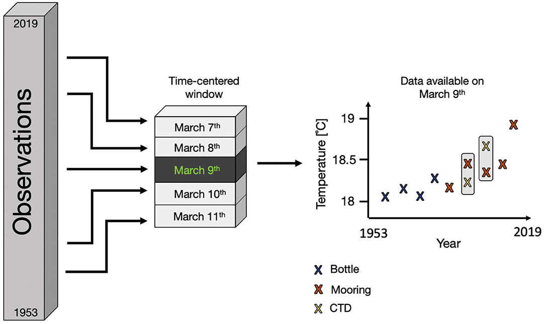
Figure 7. A visual representation of the time-centered window binning process for March 9th. Data displayed in the plot on the right that would be averaged prior to calculating climatology statistics (Date-averaging) are highlighted by the gray boxes.

4.2. Intra-Daily Variability

Most bottle and CTD data were collected in the morning, whereas mooring measurements were made every 5 min near-continuously. It was possible that this mismatch between data sources may have had an effect on climatology statistics. An average bottle data bias of approximately 0 ± 0.4°C and 0.3 ± 0.5°C was estimated for the climatological means and 90th percentiles, respectively, when comparing daily temperature statistics using mooring data between 09:00 and 11:00 only, with those calculated using mooring data over the whole day. These daily temperature statistics were calculated using data between 2009 and 2019 at a depth of 19 m. Further, to explore the possible effect of intra-daily variability on climatology statistics, the temperature diurnal cycles were investigated using mooring data between 2009 and 2019 at all climatology depth levels and for each season. The clearest diurnal cycles (calculated by subtracting the minimum daily average temperature from the maximum daily average temperature) were seen in Summer and Autumn. The largest diurnal cycle was at 19 m depth in Summer (0.7°C). At other depths in Summer and Autumn, the diurnal cycles were either less than 0.4°C (combined average of 0.2°C), or unclear. In Winter and Spring, the diurnal cycles were less clear overall, although temperatures could vary by up to 0.17°C at some depths. Overall, these diurnal cycles were approximately 7 to 64 times smaller than the intra-annual signal (see section 5), dependent on which climatology depth and season was selected, but may explain to some extent the inter-annual variability on some climatology days (particularly in summer and autumn).

The possible effect of high-frequency variability, such as internal tides, on the accuracy of climatology statistics was also explored. Temperature varied by up to 5°C within one day, and in some instances over an hour, evident in the high-resolution mooring data at depths that typically experience strong stratification. However, when considering the entire mooring record at three climatology depth levels (19, 49, and 99 m) temperature changed on average by | 0.05 | ± 0.12°C over an hour, and by | 0.17 | ± 0.28°C over a day. Therefore, hours and days when temperature varied by as much as 5°C were not representative of the usual conditions, and the effect of high-frequency variability on climatology statistics was expected to be low.

4.3. Validation of the Methodology

4.3.1. Synthetic Data

The methodology used to create the climatology was defined and tested using synthetically-created hourly temperature data. These synthetic data were created with similar statistical properties to the observed temperature data between 1953 and 2019 at depths of 17 m to 21 m depth. For each climatology day, the moments of the observed data distribution were calculated (means, standard deviation, skewness, and kurtosis). Synthetic temperatures for each day of the year between 1953 and 2019 were randomly determined from these moments (using the 60-day smoothed means and Pearson system random numbers (Johnston et al., 1994, MATLAB function “pearsrnd.m”). Inter-annual variability in the synthetic data for each climatology day resulted from the Pearson system random numbers method. Inter-decadal variability was added to the synthetic data using piece-wise linear regression and 4 time intervals: 1953 to 1970, 1970 to 1990, 1990 to 2010, and 2010 to 2019. Both the piece-wise trends and the long-term one discussed in section 4.1.5 (approximately 1°C century⁻¹ between 1953 and 2019) were computed similarly to the method used by Thompson et al. (2009). The real temperature data were seasonally de-trended by subtracting the climatological monthly averages using all temperatures between 1953 and 2019, from all available temperatures for the same month. Seasonally de-trended temperature data were then monthly-gridded, and the trends were estimated.

The observed distribution moments varied over the climatological days, with the means, standard deviations, skewness, and kurtosis ranging from 17.5 to 22.3°C (see Figure 8A), 0.3 to 3.1°C, -3 to 3, and 1 to 14, respectively, incorporating seasonality in the synthetic data. As the observed statistical moments (excluding the mean) and the associated sampling characteristics were similar throughout the water column, for simplicity only one depth range (19 ± 2 m) was used to explore the uncertainties resulting from creating a climatology with non-homogeneous observed data. The synthetic temperature time-series had an overall mean equal to the overall mean of the combined real data. Further, the overall synthetic temperature median, standard deviation, distribution skewness and kurtosis were similar to the combined real data (Table 2). Finally, when comparing real and synthetic data over three different continuous time periods: May 2012 to December 2013, February 2014 to December 2015, and March 2016 to August 2017, the spectral qualities were similar for periods of 200 days or more. We are therefore confident that these synthetic data can be used to explore the effect of different sampling patterns, and the various methodologies used to calculate climatology statistics.

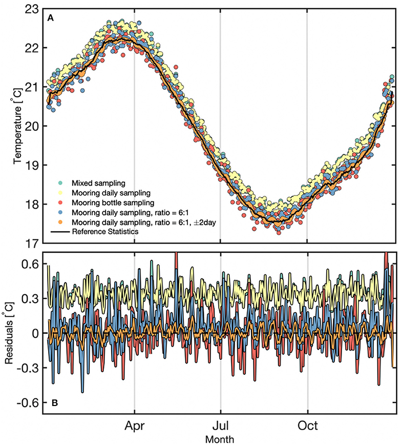
Figure 8. (A) Comparing synthetic daily temperature climatological means produced using different methods (described in section 4.3) between 17 and 21 m depth. The black line indicates the synthetic temperature climatology reference statistics. (B) The synthetic temperature residuals (or bias) between the daily reference statistics and each synthetic daily temperature climatology produced using different methods at the same depth range.

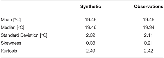
Table 2. The mean, median, standard deviation, skewness, and kurtosis for the synthetic and observed temperature overall distributions between 1953 and 2019 at depths between 17 and 21 m.

4.3.2. Reference Statistics

Calculating a synthetic climatology using all of the hourly synthetic temperatures every 1 m within 19 ± 2 m provided an estimate of the “true” synthetic environmental conditions. This synthetic climatology represented an ideal case where a mooring equipped with temperature sensors every 1 m between 17 and 21 m measured hourly between 1953 and 2019 at the Port Hacking site. In reality, such sampling resolution in time and space was not possible. Hence methodologies had to be developed to properly account for the differences in sampling between bottle, CTD, and mooring data in time and space. This calculated synthetic climatology provided reference statistics (means, 10th and 90th percentiles). Subsequent synthetic climatology statistics, calculated using different methods accounting for potential bias, were compared with the reference statistics. These reference statistics are displayed in Figure 8, which summarizes the results of the various sampling methods applied. The final methodology was chosen based on the Root Mean Square Errors (RMSEs) (listed in Table 3) calculated between the synthetic reference statistics and the ones produced using different realistic sampling patterns and methods accounting for potential bias.

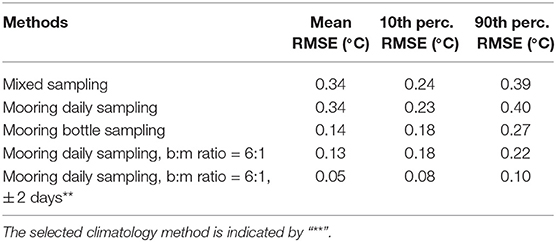
Table 3. A comparison of the temperature Root Mean Square Errors (RSMEs, °C) between the synthetic climatology statistics using different climatology methods (described in section 4.3) and the reference climatology statistics for the mean, 10th and 90th percentiles.

4.3.3. Temporal Resolution

The effect of considering similar sampling resolution in time and space to the real observations prior to dealing with any potential bias was explored (method “mixed sampling,” Figure 8). Synthetic hourly temperature data between 1953 and 2010 were subsampled randomly every 10 to 14 days resembling bottle data, whilst synthetic data between 2010 and 2019 remained at hourly resolution resembling mooring data. This “Mixed sampling” synthetic climatology had associated RMSEs of 0.24 to 0.39°C (Table 3), when considering the mean and percentiles. The “Mixed sampling” statistics were generally warmer due to an over representation of warmer synthetic temperatures between 2010 and 2019. Further, these RMSEs suggested that the mixed temporal sampling (similar to real sampling characteristics) between 1953 and 2010 might not have fully resolved the intra-annual signal at NRSPHB / PH100.

The effect of changing the mooring data temporal resolution between 2010 and 2019 was also explored using two methods; “Mooring daily sampling” using daily-averaged synthetic mooring data, and “Mooring bottle sampling” using daily-averaged synthetic mooring data subsampled every 10 to 14 days similar to real bottle observations. These synthetic mooring data were combined with the synthetic bottle data subsampled every 10 to 14 days between 1953 and 2010 to produce synthetic climatology statistics. The “Mooring daily sampling” and “Mooring bottle sampling” RMSEs ranged between 0.23 and 0.40°C, and 0.14 and 0.27°C, respectively (Table 3). The low RMSEs calculated between the reference statistics and the “Mooring bottle sampling” method suggested that it was preferential to have constant temporal resolution over the entire time period. However, larger synthetic temperature residuals were seen on some days when testing the “Mooring bottle sampling” method (Figure 8B) when compared with the “Mooring daily sampling” method, and an advantage of using the daily mooring data was the availability of data throughout the year. Further, a step that considers data consistency over the whole period was later incorporated (i.e., b:m ratio, sections 4.1.5 and 4.3.4). Therefore, a methodology incorporating daily-averaged mooring profiles was explored.

4.3.4. Data Source Ratio

Calculating climatology statistics using a bottle to mooring (b:m) binned year ratio of 6:1 was examined using synthetic temperatures subsampled every 10 to 14 days between 1953 and 2010, and daily averaged synthetic mooring data between 2010 and 2019. This b:m ratio restricted the number of synthetic mooring binned years (e.g., 2010, 2011, 2012, etc.) available for each climatology day (e.g., March 9th) relative to the total number of synthetic bottle binned years available. The smaller synthetic mooring data subsample consisted of binned years chosen at random. The RMSEs when incorporating this method were either the same or lower than the RMSEs for previous methods, suggesting that a b:m ratio of 6:1 should be used.

4.3.5. Time-Centered Moving Window

The effect of using a time-centered moving window of ± 2 climatology days in combination with a b:m ratio of 6:1 was explored using synthetic temperatures subsampled every 10 to 14 days between 1953 and 2010 (representing bottle data), and daily averaged synthetic temperature data between 2010 and 2019 (representing mooring data). This method had the lowest RMSEs (0.05°C for the mean, 0.10°C for the 90th percentiles), indicating that a time-centered moving window of ±2 days should be used in combination with a b:m ratio of 6:1 to calculate climatology statistics.

5. The Climatology

The daily ocean temperature climatology, produced using the methodology described in section 4, was useful for computing intra-annual temperature variability at the NRSPHB / PH100 site. The climatology means, 10th and 90th percentiles varied over the course of the year, and with varying depth (Figure 9). Average temperature typically varies by 4 to 6°C between 19 and 99 m late Spring to late autumn. It is during this time that waters are stratified due to more stable atmospheric conditions. Peak temperatures at depths less than 45 m can be seen early to mid-autumn. Between late Autumn and early spring, the water column is well-mixed on average, with temperature varying by 2 to 3°C between 19 and 99 m. It is because of this mixing that peak average temperatures are present in late autumn at depths greater than 45 m as warmer waters are mixed with the colder waters below. The depth threshold between early-mid autumn and late autumn temperature peaks vary for the 10th and 90th percentiles. This depth threshold was approximately 45 m for average temperatures, but approximately 49–74 m and 35 m for the 90th and 10th percentiles, respectively.

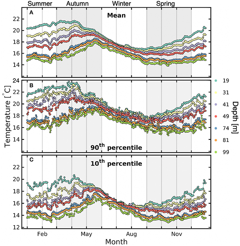
Figure 9. The climatology (A) means, (B) 90th and (C) 10th percentiles for each optimal depth level: 19, 31, 41, 49, 74, 81, and 99 m. The alternating gray shading present in time-depth plot space in each subpanel represents the different seasons, labeled at the top of panel (A).

Each daily climatological mean had a corresponding standard deviation displayed in Figure 10 for each climatology day and depth. These standard deviations varied between 0.5°C and 2°C, and were on average 1.06°C when considering all climatology days and depth levels. The standard deviations were related to both the data characteristics and the natural variability at this site, and were generally higher in Summer and Autumn when there was increased stratification, and lower in Winter and Spring when there was increased mixing.

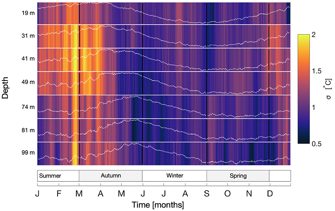
Figure 10. The temperature climatology standard deviations (σ) are shown as constant bars for each day of the year and climatology depth. Note the varying intervals between climatology depths. The normalized mean temperatures (see Figure 9A for values) are superimposed over the standard deviations as white dashed lines for each climatology depth. The seasons are labeled below the plot area along with corresponding black vertical lines signifying a change of season, shown for each climatology depth.

The daily ocean temperature climatology is useful for determining periods of anomalously high or low temperatures [e.g., marine heatwaves (MHWs), Schaeffer and Roughan, 2017]. As the climatology is subsurface, the effect of extreme temperature below the surface at this site can be explored. Schaeffer and Roughan (2017) showed that in this region MHWs are subsurface intensified, hence the subsurface information is useful. Further, producing a daily temperature climatology at this site has allowed for the delayed-mode identification of extremes at the Port Hacking site, which has been delivered as a web-based app (http://www.oceanography.unsw.edu.au/).

6. Conclusion

A daily ocean temperature climatology data product has been produced at the NRSPHB / PH100 site approximately 6 km offshore from the greater Sydney region, Australia using a combination of bottle, CTD, and mooring data between 1953 and 2019. Calculating a climatology using temperature data sets obtained via different methods, and with varying temporal and vertical resolution required careful consideration so as to avoid biases. The seven steps used to create the climatology are summarized here:

1. Confirm the implementation of automatic QC as per the required standards

2. Quality control the data sets to a similar standard. Automatic QC tests applied to bottle, CTD, and mooring data that consider 1. outliers outside of a defined threshold, 2. shallow / deep profiles, 3. spatial proximity to the NRSPHB / PH100 nominal locations, and 4. profiles with more than 30% of data flagged.

3. Combine quality controlled daily bottle, CTD, and mooring temperature profiles spanning 1953 to 2019.

4. Determine the optimal depths used to calculate climatology statistics based on the distribution of two or more data sources throughout the water column that have different sampling characteristics.

5. Linearly interpolate temperature profiles vertically and temporally based on scales of variability, within the range of a profile's shallowest and deepest observations.

6. Account for differing data source sampling frequencies by enforcing a data source observed year ratio (in our case, a bottle to mooring ratio of 6:1), incorporating daily temperatures within a time-centered moving window, and taking into consideration dates when more than one data source is available. As the mooring binned years were chosen at random whilst implementing the bottle to mooring ratio, a possible improvement may be to calculate statistics using an ensemble of bottle / mooring binned year combinations.

7. Test the climatology methodology using synthetic temperature data with similar qualities to real observations. Although considered a last step here, the decisions leading to the steps above were aided by the testing of methodologies using these synthetic data.

Producing a daily temperature climatology at NRSPHB / PH100 highlighted the importance of having an Integrated Marine Observing System (IMOS). The foresight to continue temperature measurements post 2009 at NRSPHB / PH100 meant better data coverage in depth and time, and an ability to identify recent temperature extremes using a suitable climatology baseline period that included the last 10 years. There is a large spectrum of uses for an ocean observing system, from looking at small-scale variability (e.g., internal tides) requiring high-resolution spatial and temporal data, to long-term ocean monitoring (e.g., trend analysis) requiring consistent long-term sampling. It is challenging for an ocean observing system to meet all of the demands of its data users. However, if the sole purpose of an ocean observing system is to produce a climatology, the following suggestions identified during the climatology methodology process may be useful in aiding its design: (1) Maintain consistent vertical resolution in time, with adequate vertical spacing (ideally covering the thermocline) determined using typical scales of variability if available (e.g., determined from autocorrelation analysis). If the observing system is an addition to an existing network of observation platforms (e.g., moorings and ship tracks), ensure that any new measurements are made at similar depths. This maximizes the number of depth levels at which the climatology can be produced. (2) Maintain consistent time intervals throughout time. Temporal resolution should be equal to or higher than the time resolution of the climatology that you wish to produce (e.g., in our case, daily resolution or higher). This ensures that data are available throughout the observation period at each climatology time interval. (3) Maintain similar sensor technology throughout time. Changing the sensor type used at a site could cause data discontinuities or changes in data quality. Using similar sensor technology throughout the observation period would increase the utility of the data.

Although this methodology was applied to a single site, many of the methodology steps can be readily applied to a range of site locations, or on a global scale. For example, the QC tests applied to the bottle, CTD, and mooring data might be useful for globally-available data sets. We have described a method that is useful for accounting for the different sampling characteristics of a range of data sources, and we have illustrated how the method can be tested using synthetic data. The methodology presented here can be adopted and adapted at other sites across Australia and worldwide where similar multiple source data sets exist.

Data Availability Statement

Publicly available data sets were used for this study. The mooring and CTD data were accessed from the Integrated Marine Observing System (IMOS) Australian Ocean Data Network (AODN) portal here: https://portal.aodn.org.au/. IMOS is enabled by the National Collaborative Research Infrastructure Strategy (NCRIS). It is operated by a consortium of institutions as an unincorporated joint venture, with the University of Tasmania as Lead Agent. The bottle data were accessed from the CSIRO Marine and Atmospheric Research Laboratories Information (MarLIN) Network portal here: http://www.marine.csiro.au/marq/edd_search.Browse_Citation?txtSession=5301&brief=Y.

Author Contributions

MR devised the climatology. MH and AS conducted the methodology and analysis. MH and MR wrote the manuscript. MH produced the figures and tables. All authors reviewed the manuscript.

Funding

The multi-decadal data collection has been co-funded by the Australian Commonwealth Scientific and Industrial Research Organisation (CSIRO), the New South Wales Department of Planning, Industry and Environment (formerly Office of Environment and Heritage, OEH), and the Integrated Marine Observing System (IMOS). MH is funded by UNSW Sydney as a contribution to IMOS.

Conflict of Interest

The authors declare that the research was conducted in the absence of any commercial or financial relationships that could be construed as a potential conflict of interest.

Acknowledgments

We thank Guillaume Galibert for his contribution to an early version of the climatology methodology. We are very grateful to everyone involved in the data collection, including: C. Holden (Oceanographic Field Services Pty Ltd), the NSW-IMOS moorings team for the on-going mooring deployments, T. Austin, S. Milburn, and B. Morris for their hard work on mooring field campaigns, T. Austin for processing the mooring and CTD data, and T. Ingleton and his team for their ongoing involvement in the PH100 / NRSPHB sampling. We acknowledge everyone who has been involved in hydrographic sampling since 1953 and the foresight of CSIRO Marine Research for instigating and continuing the data collection. In particular we acknowledge the NSW Department of Planning, Industry and Environment who presently lead the monthly sampling. Data were sourced from Australia's Integrated Marine Observing System (IMOS) - IMOS is enabled by the National Collaborative Research Infrastructure Strategy (NCRIS). It is operated by a consortium of institutions as an unincorporated joint venture, with the University of Tasmania as Lead Agent. Finally, we thank 3 reviewers for providing comments that helped to improve the manuscript.

References

Abraham, J. P., Baringer, M., Bindoff, N., Boyer, T., Cheng, L., Church, J., et al. (2013). A review of global ocean temperature observations: implications for ocean heat content estimates and climate change. Rev. Geophys. 51, 450–483. doi: 10.1002/rog.20022
Bailey, K., Steinberg, C., Davies, C., Galibert, G., Hidas, M., McManus, M., et al. (2019). Coastal mooring observing networks and their data products: recommendations for the next decade. Front. Mar. Sci. 6:180. doi: 10.3389/fmars.2019.00180
Benway, H. M., Lorenzoni, L., White, A. E., Fiedler, B., Levine, N. M., Nicholson, D. P., et al. (2019). Ocean time series observations of changing marine ecosystems: an era of integration, synthesis, and societal applications. Front. Mar. Sci. 6:393. doi: 10.3389/fmars.2019.00393
Buck, J., Bainbridge, S. J., Burger, E. F., Kraberg, A., Casari, M., Darroch, L., et al. (2019). Ocean data product integration through innovation-the next level of data interoperability. Front. Mar. Sci. 6:32. doi: 10.3389/fmars.2019.00032
Dunn, J. (2011). CSIRO Atlas of Regional Seas (CARS). Available online at: http://www.marine.csiro.au/~dunn/cars2009/#refs
Gouretski, V. (2018). World ocean circulation experiment-argo global hydrographic climatology. Ocean Sci. 14, 1127–1146. doi: 10.5194/os-14-1127-2018
Gouretski, V., and Jancke, K. (1999). A description and quality assessment of the historical hydrographic data for the South Pacific Ocean. J. Atmos. Ocean. Technol. 16, 1791–1815. doi: 10.1175/1520-0426(1999)016<1791:ADAQAO>2.0.CO;2
Hobday, A. J., Alexander, L. V., Perkins, S. E., Smale, D. A., Straub, S. C., Oliver, E. C., et al. (2016). A hierarchical approach to defining marine heatwaves. Prog. Oceanog. 141, 227–238. doi: 10.1016/j.pocean.2015.12.014
Ingleton, T., Morris, B., Pender, L., Darby, I., Austin, T., and Galibert, G. (2014). Standardised Profiling CTD Data Processing Procedures V2.0. Sydney, NSW: Integrated Marine Observing System.
Iwamoto, M. M., Dorton, J., Newton, J. A., Yerta, M., Gibeaut, J. C., Shyka, T., et al. (2019). Meeting regional, coastal and ocean user needs with tailored data products: a stakeholder-driven process. Front. Mar. Sci. 6:290. doi: 10.3389/fmars.2019.00290
Johnston, N., Kotz, S., and Balakrishnan, N. (1994). Continuous Univariate Distributions (Vol. 1). New York, NY.
Kerry, C., Powell, B., Roughan, M., and Oke, P. (2016). Development and evaluation of a high-resolution reanalysis of the East Australian Current region using the Regional Ocean Modelling System (ROMS 3.4) and Incremental Strong-Constraint 4-Dimensional Variational (IS4D-Var) data assimilation. Geosci. Model Dev. 9, 9779–3801. doi: 10.5194/gmd-9-3779-2016
Lauvset, S. K., Key, R. M., Olsen, A., van Heuven, S., Velo, A., Lin, X., et al. (2016). A new global interior ocean mapped climatology: the 1 ×1 GLODAP version 2. Earth Syst. Sci. Data 8, 325–340. doi: 10.5194/essd-8-325-2016
Levitus, S. (1983). Climatological atlas of the world ocean. EOS Trans. Am. Geophys. Union 64, 962–963. doi: 10.1029/EO064i049p00962-02
Locarnini, R., Mishonov, A., Baranova, O., Boyer, T., Zweng, M., Garcia, H., et al. (2019). World Ocean Atlas 2018, Volume 1: Temperature. A. Mishonov Technical Ed (Silver Spring, MD: National Oceanic and Atmospheric Administration).
Lynch, T., Morello, E., Middleton, J., Thompson, P., Feng, M., Richardson, A., et al. (2011). National Reference Station (NRS) Network: Rationale, Design and Implementation Plan. IMOS. Available online at: http://imos.org.au/fileadmin/user_upload/shared/ANMN/NRS_rationale_and_implementation_100811.pdf
Lynch, T. P., Morello, E. B., Evans, K., Richardson, A. J., Rochester, W., Steinberg, C. R., et al. (2014). IMOS National Reference Stations: a continental-wide physical, chemical and biological coastal observing system. PLoS ONE 9:e113652. doi: 10.1371/journal.pone.0113652
Morello, E. B., Galibert, G., Smith, D., Ridgway, K. R., Howell, B., Slawinski, D., et al. (2014). Quality control (QC) procedures for Australia's National Reference Station's sensor data–comparing semi-autonomous systems to an expert oceanographer. Methods Oceanogr. 9, 17–33. doi: 10.1016/j.mio.2014.09.001
Oliver, E. C., Donat, M. G., Burrows, M. T., Moore, P. J., Smale, D. A., Alexander, L. V., et al. (2018). Longer and more frequent marine heatwaves over the past century. Nat. Commun. 9:1324. doi: 10.1038/s41467-018-03732-9
Olsen, A., Key, R. M., Van Heuven, S., Lauvset, S. K., Velo, A., Lin, X., et al. (2016). The Global Ocean Data Analysis Project version 2 (GLODAPv2)-an internally consistent data product for the world ocean. Earth System Science Data 8, 297–323. doi: 10.5194/essd-8-297-2016
Ridgway, K., Dunn, J., and Wilkin, J. (2002). Ocean interpolation by four-dimensional weighted least squares–application to the waters around Australasia. J. Atmos. Ocean. Technol. 19, 1357–1375. doi: 10.1175/1520-0426(2002)019<1357:OIBFDW>2.0.CO;2
Rochford, D. J. (ed.). (1951). Oceanographic Station List: Onshore Hydrological Investigations in Eastern Australia, Vol. 4. Melbourne, VIC: CSIRO.
Roughan, M., and Morris, B. D. (2011). “Using high-resolution ocean timeseries data to give context to long term hydrographic sampling off Port Hacking, in Oceans'11 MTS/IEEE Kona (Kona, HI: IEEE), 1–4. doi: 10.23919/OCEANS.2011.6107032
Roughan, M., Schaeffer, A., and Kioroglou, S. (2013). “Assessing the design of the NSW-IMOS moored observation array from 2008-2013: recommendations for the future, in 2013 OCEANS-San Diego (San Diego, CA: IEEE), 1–7.
Roughan, M., Schaeffer, A., and Suthers, I. M. (2015). “Sustained ocean observing along the coast of southeastern Australia: NSW-IMOS 2007-2014, in Coastal Ocean Observing Systems (London: Elsevier), 76–98. doi: 10.1016/B978-0-12-802022-7.00006-7
Sabine, C. L., Hankin, S., Koyuk, H., Bakker, D. C. E., Pfeil, B., Olsen, A., et al. (2013). Surface ocean CO2 Atlas (SOCAT) gridded data products. Earth Syst. Sci. Data 5, 145–153. doi: 10.5194/essd-5-145-2013
Schaeffer, A., and Roughan, M. (2017). Subsurface intensification of marine heatwaves off southeastern Australia: The role of stratification and local winds. Geophys. Res. Lett. 44, 5025–5033. doi: 10.1002/2017GL073714
Schaeffer, A., Roughan, M., Jones, E. M., and White, D. (2016). Physical and biogeochemical spatial scales of variability in the East Australian Current separation from shelf glider measurements. Biogeosciences 13, 1967–1975. doi: 10.5194/bg-13-1967-2016
Schaeffer, A., Roughan, M., and Morris, B. D. (2013). Cross-shelf dynamics in a western boundary current regime: Implications for upwelling. J. Phys. Oceanogr. 43, 1042–1059. doi: 10.1175/JPO-D-12-0177.1
Schlegel, R. W., Oliver, E. C., Wernberg, T., and Smit, A. J. (2017). Nearshore and offshore co-occurrence of marine heatwaves and cold-spells. Prog. Oceanogr. 151, 189–205. doi: 10.1016/j.pocean.2017.01.004
Sutherland, M., Ingleton, T., and Morris, B. (2017). Pre-Run Check and Field Sampling CTD Procedural Guide V3.0. Coasts and Marine Team, New South Wales Office of Environment and Heritage, Sydney and Sydney Institute of Marine Science, Sydney, NSW.
Thompson, P., Baird, M., Ingleton, T., and Doblin, M. (2009). Long-term changes in temperate Australian coastal waters: implications for phytoplankton. Mar. Ecol. Prog. Ser. 394, 1–19. doi: 10.3354/meps08297
UNESCO (2019). United Nations Decade of Ocean Science for Sustainable Development (2021-2030). Available online at: https://www.oceandecade.org/
Union Nations (2015). Transforming our World: The 2030 Agenda for Sustainable Development. General Assembley 70 session.
Visbeck, M., Kronfeld-Goharani, U., Neumann, B., Rickels, W., and Schmidt, J. (2014). Securing blue wealth: the need for a special sustainable development goal for the ocean and coasts and for future ocean spatial planning. Mar. Policy 48:184. doi: 10.1016/j.marpol.2014.03.005
Wijffels, S. E., Beggs, H., Griffin, C., Middleton, J. F., Cahill, M., King, E., et al. (2018). A fine spatial-scale sea surface temperature atlas of the Australian regional seas (SSTAARS): seasonal variability and trends around Australasia and New Zealand revisited. J. Mar. Syst. 187, 156–196. doi: 10.1016/j.jmarsys.2018.07.005
Keywords: data product, East Australian Current, daily climatology, subsurface, multi-platform, data aggregation, Australia, Port Hacking
Citation: Hemming MP, Roughan M and Schaeffer A (2020) Daily Subsurface Ocean Temperature Climatology Using Multiple Data Sources: New Methodology. Front. Mar. Sci. 7:485. doi: 10.3389/fmars.2020.00485
Received: 02 December 2019; Accepted: 29 May 2020;
Published: 30 July 2020.
Edited by:
Johannes Karstensen, GEOMAR Helmholtz Center for Ocean Research Kiel, GermanyReviewed by:
Simona Simoncelli, National Institute of Geophysics and Volcanology (Bologna), ItalyStephanie Guinehut, Collecte Localisation Satellites (CLS), France
Eisuke Tsutsumi, University of Tokyo, Japan
Copyright © 2020 Hemming, Roughan and Schaeffer. This is an open-access article distributed under the terms of the Creative Commons Attribution License (CC BY). The use, distribution or reproduction in other forums is permitted, provided the original author(s) and the copyright owner(s) are credited and that the original publication in this journal is cited, in accordance with accepted academic practice. No use, distribution or reproduction is permitted which does not comply with these terms.
*Correspondence: Michael P. Hemming, m.hemming@unsw.edu.au