Rock slope displacement prediction based on multi-source information fusion and SSA-DELM model

Introduction

In the construction of mountain housing, transportation, mining, water conservancy and hydropower projects, rock slope stability problems are inevitably encountered (Li et al., 2019; Du et al., 2022; Yi et al., 2022; Zhao et al., 2022). Rock slope stability problems can cause geological disasters such as rock loosening, relaxation cracking, creeping, landslides and rock fall (Liu et al., 2020; Meng et al., 2021; Xu et al., 2022). Therefore, monitoring and early warning are pivotal in preventing rock slope disasters. In rock slope disaster monitoring and early warning, the research is often conducted on static indicators (such as deformation, stress, etc.)or environmental indicators (such as groundwater, rainfall, etc.) (Du et al., 2019), among which displacement is an intuitive and reliable monitoring quantity under the influence of internal and external environment. The scientific analysis of displacement data and the establishment of real-time prediction models are essential research contents in large-scale engineering safety monitoring.

In order to obtain accurate, comprehensive, and real-time information on landslide deformation, it is necessary to monitor both surface and subsurface deformation, as well as triggering factors and related environmental factors, so multiple means of landslide monitoring must be used simultaneously to achieve effective monitoring results (Zhang et al., 2020). Nowadays, the techniques applied in mainstream rock slope monitoring include synthetic aperture radar (Pieraccini et al., 2006; Atzeni et al., 2015; Qin et al., 2020), microseismic monitoring (Salvoni and Dight., 2016; Xu et al., 2016; Ma et al., 2017; Chen et al., 2022), GNSS displacement monitoring (Lian et al., 2020; Šegina et al., 2020; Yan et al., 2022), etc. These monitoring techniques mainly focus on the surface and deep deformation of rock slopes, and some scholars also combine environmental quantity indicators for monitoring and research, such as Pang (Pang, 2019) proposed an automated monitoring system, which contains GPS monitoring station, rain gauge, crack gauge, rain gauge, groundwater level gauge and other sensors to monitor the slope in real-time, which can respond to the slope deformation parts in time with a broader perspective to ensure the safety of high-risk slopes and their surroundings; Liu et al. (Liu et al., 2022) combined slope deformation monitoring data, displacement monitoring data, inclination monitoring data, groundwater level monitoring data, rainfall monitoring data and other multi-source data, based on machine learning method to monitor abnormal events of monitoring data to provide support for disaster early warning; Peng et al. (Peng et al., 2014) combined multiple sensor monitoring data and multiple mechanical parameters to update soil or rock model parameters, slope safety coefficients and damage efficiency using Markov chain Monte Carlo simulation, which made the assessment more reliable; Li et al. (Li et al., 2021) combined field experiments and blasting vibration monitoring to systematically study the three-dimensional dynamic stability of adjacent high slopes after blasting vibration, providing technical support and theoretical guidance for mine blasting and improving mine stability.

The use of multiple sensors to monitor slopes can obtain a large amount of multi-source heterogeneous data, which have specific correlation, randomness, and ambiguity (Wang et al., 2020). How to fully use these multi-source heterogeneous data is the focus of scholars’ attention and the problems that have been needed. Over the past few years, the multi-source data fusion method has been increasingly favored by some experts and scholars in the field of slope research, and it has begun to be gradually applied in engineering. Some scholars have used multi-source data fusion technology for the prediction and stability analysis of slope safety factor (Sakellariou and Ferentinou., 2005; Liu et al., 2014.; Jiang et al., 2022), and some scholars at home and abroad have used multi-source heterogeneous data fusion technology for risk warning and analysis of landslides to study the characteristic mechanism and dynamics evolution law of the deformation and damage process of landslides (Du et al., 2020; Zhang et al., 2020; Li et al., 2021). In recent years, multi-source data fusion techniques have been more successfully applied to landslide displacement prediction. Liu et al. (Liu et al., 2020) introduced two concepts, trend sequence and sensitivity, to quantitatively characterize landslide displacement caused by external factors and internal landslide state, respectively, and proposed a nonlinear model for landslide displacement prediction by fusing trend sequence and sensitivity state; Wang et al. (Wang et al., 2021) used Pearson correlation coefficient, and mutual information were used to screen environmental factors and deep learning was used to predict landslide displacements; Duan et al. (Duan et al., 2017) used comprehensive landslide monitoring data to extract the most relevant factors affecting landslide deformation and used an autoregressive integrated movement model for prediction. Wang and Zhang (Wang et al., 2022; Zhang et al., 2022) considered the hydrodynamic effects affecting landslides, used a variational modal decomposition method to decompose the cumulative displacement into the trend, periodic and stochastic terms, and used different deep learning methods to make predictions for three Different deep learning methods are used to predict the three different displacement subterms.

Scholars have rarely considered the relationship between the dependent variables in the prediction of landslide displacement using multi-source heterogeneous data of slopes, which can lead to overfitting and low prediction accuracy in the prediction. Nowadays, the mainstream methods of variable selection mainly include correlation analysis (Guo et al., 2022), mutual information (Li, 2021), and lasso (Jin et al., 2021). However, these methods are relatively single, and it is difficult to select the appropriate number of variables when screening the variables, and too few input variables will lead to lower prediction accuracy. On the other hand, too many input variables will result in redundant variables and increase the model running time.

In the past, scholars did not consider the redundancy among the dependent variables when using multi-source heterogeneous data of slopes for landslide displacement prediction, leading to overfitting and low prediction accuracy. To this end, this paper proposes a method of variable selection by combining Pearson correlation and gray correlation analysis. The Pearson correlation analysis is used to calculate the correlation coefficients of each variable factor, judging whether there are uncorrelated or redundant relationships among them. Then the model combines the correlation coefficients between variables and displacement to eliminate redundant variables. Finally, the sparrow search algorithm optimized by the depth limit learning machine is utilized to predict displacement, which provides a reference for the subsequent displacement change and reduces the occurrence of slope disaster.

Principles of algorithms

Pearson correlation analysis

Karl Pearson introduced the Pearson correlation coefficient (PCC) in the 1880s. The correlation coefficient determines whether each input variable is closely correlated with each other, and if two variables are highly correlated with each other, they belong to duplicate features and can be removed to achieve de-duplication or dimensionality reduction (Lin et al., 2019). The Pearson correlation coefficient is then expressed as follows:

Where $r$ is the Pearson correlation coefficient; $x_i$ is the different value corresponding to the variable $x$; is the average of the variables $x$;$y_i$ is the different value corresponding to the variable $y$; is the average of the variables $y$; $N$is the number of variables. The value range of the correlation coefficient is [-1.1]. When $\left|r\right|$>0, it is a positive correlation; conversely, it is a negative one. The magnitude of the absolute value of the corresponding Pearson correlation coefficient between two variables determines the strength of the relationship between the two variables, and the specific range of values and their representative meanings are shown in Table 1.

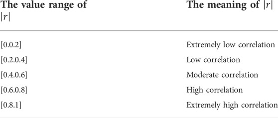
TABLE 1. The value range of $\left|r\right|$and its meaning.

Gray relational analysis

Gray relational analysis theory, an essential part of gray system theory, is a multifactor statistical analysis theory that describes the strength, magnitude, and order among factors in terms of gray correlation degree based on sample data of each factor. Gray correlation is essentially a comparison of how close the geometric shapes of the data curves are. The closer the geometry, the closer the trend of change and the greater the correlation (Liu et al., 2012). The analysis steps are as follows:

Step1. Identify the mother series and characteristic series. Generally, the dependent variable is determined as the mother series, and the independent variable is determined as the characteristic series. In this paper, the landslide displacement is determined as the mother series, and the landslide impact factor is determined as the characteristic series.

Step2. Undimensionalize the data. The dimensionless processing is typically done by initialization, homogenization, and normalization, and this paper uses normalization for the dimensionless processing of data. The calculation formula of normalization is then expressed as follows:

Where $X$is the raw data; $X_{\max }$, $X_{\min }$ are respectively the maximum and minimum values of the data.

Step3. Solve for the gray relational coefficient value between the parent sequence and the feature sequence. The relational coefficient represents the degree of correlation between the feature series and the mother series in the corresponding dimension, and the larger the number, the stronger the correlation. The calculation formula of the correlation coefficient is then expressed as follows:

Where ${\xi }_e\left(k\right)$ is the value of correlation coefficients of feature sequence $x_e$ to feature sequence $x_0$ on the $kth$ indicator.

Step4. Calculate the correlation between the mother sequence and the feature sequence. Larger correlation degree proves that the corresponding feature sequence has more influence on the mother sequence. The calculation formula of correlation degree is then expressed as follows:Where $n$ is the sample size; $r_{\epsilon }$ is the correlation degree of feature sequence, and the indicator weight.

Sparrow search algorithm

The Sparrow Search Algorithm (SSA) is a relatively novel algorithm inspired by the foraging and anti-predatory behaviors of sparrows (Xue and Shen., 2020), which has the advantages of merit-seeking solid ability, fast convergence, and robustness. The bionic principle is as follows:

When sparrows search for food, they need to divide the whole sparrow population into three categories according to their different divisions of labor: producers searching for food, joiners grabbing food of their kind, and vigilantes finding enemies. Producers are generally the highest energy sparrows in the whole population because they need to search for food and guide the direction of the population. In continuous iteration, producers and joiners can transform each other, but the proportion of the two species in the whole population will not change in the transformation process. In the bionic experiment, the sparrow population and fitness values need to be initialized first, and the sparrow population and fitness value initialization expressions are then expressed as follows:

Where $n$ is the number of sparrows; $d$ is the dimension of the variable to be optimized, which is the number of independent parameters; $x_{n,d}$is the value of the $nth$ sparrow in the $dth$ dimension.

After determining the location and fitness value of each sparrow, the initial fitness value of each sparrow needs to be sorted, the sparrows with the better fitness value will be identified as the producer. The producer can be given priority to obtain food when food is found and guide the whole group to the direction of food. The producer will continue to search for food in different places elsewhere, the location will keep changing, and the movement rules will also change when the enemy is encountered, at the moment, the producer location update rules are then expressed as follows:

Where $t$ is the current number of iterations; $j\in \left\{\mathrm{1,2,3},\cdots ,d\right\}$;$x_{i,j}^t$is the value of the $ith$ dimension of the $jth$ sparrow at the $tth$ iteration; $\alpha \in (\mathrm{0,1}]$, is a random number; $ite{r}_{\max }$ is the maximum number of iterations; $R_2\in \left[\mathrm{0,1}\right]$, is the alarm value; $ST\in \left[\mathrm{0,1}\right]$, is the safety threshold; $Q$ is a random number that follows a normal distribution; $L$ is a matrix of order $1\times d$(all elements are 1). When $R_2<ST$, it means that there are no natural predators in the area, which means that the area is safe and the producer will continue to expand its foraging range; when $R_2>ST$, it means that the producer has found a predator and warned other sparrows that all sparrows need to leave the area for a safe area.

For the joiners, the producers are monitored at all times, and if the producers find food, the joiners will immediately be aware of it and quickly fly to the food source to grab the food with the producer. At this time, the joiners’ position update rule is then expressed as follows:

Where $x_p$ is the best position occupied by the producer; $x_{worst}$ is the global worst position; $A$ is the matrix of order $1\times d$, each element is randomly 1 or -1;$A^{+}=A^T{\left(A{A}^T\right)}^{-1}$; When $i>\frac{n}{2}$, it means that the less adaptive first joiner fails to grab food and needs to change its position to get food in other areas.

Alerters are randomly generated in the entire population, usually 10–20% of the entire population. The initial position is then randomly generated, with the rule is then expressed as follows:

Where $f_i$ is the current sparrow adaptation value; $f_g$ is the global best adaptation value; $f_w$ is the global worst adaptation value; $\beta$ is the step control function, which is a normally distributed random number with mean 0 and variance 1; $K$ is the direction of sparrow movement; $\epsilon$ is the minimum constant, avoiding zero denominator; $x_{best}$ is the global best position; $x_{worst}$ is the global worst position. When $f_i>f_g$, it means that the vigilantes are located at the edge of the whole population and will fly to the safe area when scouting for enemies; When $f_i=f_g$, it means that the vigilantes in the centre of the population are aware of the danger and will fly to the other sparrows to avoid the danger.

Deep Extreme Learning Machine

An extreme learning machine is a single hidden layer feedforward neural network (Sulandri et al., 2021). Unlike the traditional gradient-based feedforward neural network algorithm, the input weights and thresholds of the hidden layer of the extreme learning machine network are randomly generated in the training process. Therefore, only the generalized inverse matrix theory can be used to calculate the output weights to complete the learning. Therefore, ELM network has the advantages of fast learning speed and strong generalization ability. However, because ELM is a single hidden layer structure, it cannot capture the effective features of the data in the case of high data, and high dimensionality of data. So more scholars use DELM (Tuerxun et al., 2021), which is a derivative algorithm of ELM.

Deep Extreme Learning Machine (DELM) is an ELM derivative algorithm that improves the network’s representational capability by superimposing an Extreme Learning Machine-Autoencoder (ELM-AE) to construct a multilayer network structure. When the ELM is confronted with input and output variables with an excessive amount of input data and high dimensionality, it solves the problem that an extreme learning machine with only one hidden layer cannot capture the effective features of the data (Sulandri et al., 2021). DELM is a combination of an extreme learning machine and an autoencoder, which constitutes an extreme learning machine-autoencoder, and the ELM-AE structure is shown in Figure 1.

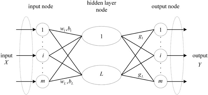
FIGURE 1. ELM-AE network structure diagram.

ELM-AE is a general approximator characterized by enabling the output of the network to be the same as the input and the input parameters of the hidden layer to be orthogonal after random generation. The output of ELM-AE can be then as follows:

Where $a$ is the matrix composed of $a_i$ , and $b$ is the vector composed of $b_i$. The output weights of the hidden layer are then expressed as follows:

Where $X=\left[X_1,X_2,X_3,\cdots X_N\right]$ is the input data.

Because of its feature representation capability, ELM-AE is used as the basic unit of the deep extreme learning machine DELM. Like traditional deep learning algorithms, DELM also uses a layer-by-layer greedy training method to train the network, and the input weights of each hidden layer of DELM are initialized using ELM-AE to perform hierarchical unsupervised training, but unlike traditional deep learning algorithms, DELM does not need reverse fine-tuning process. The structure of DELM is shown in Figure 2.

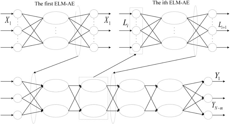
FIGURE 2. DELM structure diagram.

Assuming that the model has N hidden layers, the first output weight matrix ${\beta }_1$ is obtained from the input data X according to ELM-AE theory and then the feature vector of the hidden layer $H^1$. The output weight matrix ${\beta }_N$ of N layers and the feature vectors $H^N$ of the hidden layers can be obtained. As shown in Figure 3, the DELM first uses multiple ELM-AEs for unsupervised pre-training and then uses the output weights of each ELM-AE to initialize the whole DELM. During the ELM-AE training process, the input layer weights and thresholds are randomly generated orthogonal random matrices; meanwhile, the ELM-AE unsupervised training process uses the least squares method to update the parameters. However, in this process, only the output layer weight parameters are updated, while the input layer weights and thresholds are fixed, which will result in the prediction accuracy of the DELM being affected by the random input weights and random thresholds of each ELM-AE. Therefore, it is necessary to optimize these two parameters.

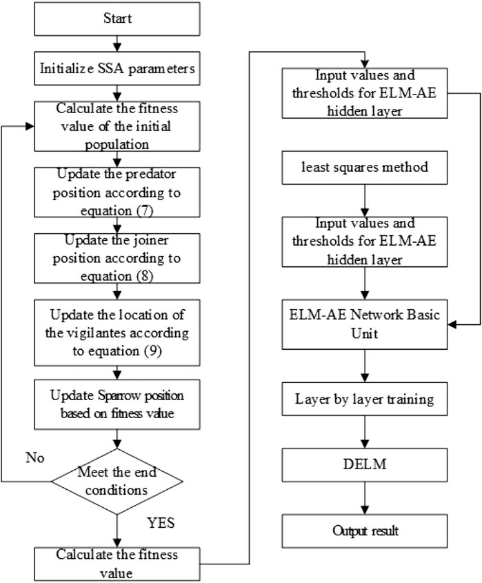
FIGURE 3. SSA-DELM flow chart.

Establishment of SSA-DELM predict model

Multiple ELM-AEs stack DELM, and the input weights and random thresholds in ELM-AEs are randomly generated, leading to random variables in the DELM model and unstable results. So these two parameters are iteratively optimized by the SSA algorithm, giving the whole model high prediction accuracy and fast convergence, which can well ensure the stability of the results. The optimization process and flow chart (Zeng et al., 2021) are then as follows.

1) Initialize the SSA algorithm parameters. Set the maximum number of training iterations, the number of sparrow populations, the alert threshold, the proportion of discoverers, and the proportion of alerters.

2) Calculate the initial fitness value of the sparrow population. Then, the sparrows with the current best and worst fitness values are selected along with their locations.

3) The positions of predators, joiners, and vigilantes are continuously updated according to Eqs 7–9.

4) After updating the positions, calculate the optimal and worst fitness values of the whole population and their positions, determine whether the maximum number of iterations is satisfied or the stopping condition is met, and if the condition is fulfilled, output the optimal value, otherwise, return to step 2).

5) The obtained results are input into the DELM model to calculate the input values and thresholds of the optimal hidden layer.

Landslide displacement modeling based on PCC-GRA-SSA-DELM

There are various manifestations of rock slope deformation, and landslide displacement is one of them. In this paper, we will combine actual engineering cases and literature, collect multiple sensor data and multiple environmental factors affecting rock slope displacement as the input parameters of SSA-DELM prediction model, and take displacement as the output parameters of the model. Since the redundancy among the factors will reduce the accuracy of the prediction model, this paper uses Person correlation analysis to calculate the correlation coefficients of the influencing factors. It then uses gray correlation analysis to calculate the correlation between the influencing factors and the landslide displacements to eliminate redundant and uncorrelated variables between them. The screened out in the prediction model, the rock slope displacement prediction model based on the PCC-GRA-SSA-DELM model is established based on four steps: data collection, data processing, variable selection, and result prediction. In this case, the obtained results are more accurate. The calculation process (as shown in Figure 4) is as follows:

1) Data collection. Multiple data sources are collected from the slope monitoring system, including displacement data, meteorological data, mechanics-related data, etc.

2) Normalizing the experimental data. Normalization limits the preprocessed data to a certain range eliminates the undesirable effects caused by odd sample data and performs inverse normalization after the model output results.

3) Variable selection. The correlation coefficients of the influencing factors were firstly calculated by using Person correlation analysis to judge the redundancy degree among the factors, and then the correlation degree between the influencing factors and landslide displacement was calculated by using gray correlation analysis, and the redundant variables and unrelated variables among them were eliminated by comprehensive comparison.

4) Result prediction. The samples are applied in the trained SSA-DELM model, the predicted values are output, and the feasibility and accuracy of the results are analyzed and verified.

5) Evaluation metrics. In this paper, the mean absolute error (MAE), and the mean square error (RMSE) are taken as the evaluation indexes of the model and calculated as follows:

Where $N$ is the number of samples predicted; $y_i$ is the actual value of displacement; ${\widehat{y}}_i$ is the predicted value of displacement.

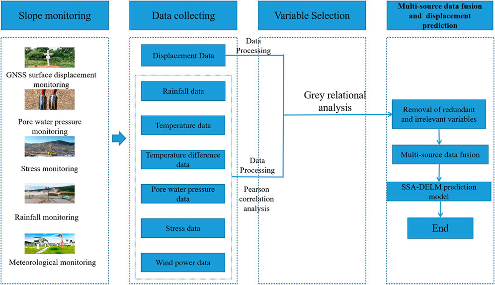
FIGURE 4. PCC-GRA-SSA-DELM model prediction flow chart.

Numerical calculation and analysis

Introduction of case projects

A cement mine in Fengxiang District is located in Fengxiang District, Baoji City, Shaanxi Province, China, at latitude 34°32′43″-34°32′54″N and longitude 107°30′26″-107°30′57″E. The quarry slope is mainly composed of the Devonian medium-thick laminated hard tuff rock group, with tangential slope and reverse slope, which is more favorable to the stability of the slope, with good stability of the slope in general, and not easy to produce large-scale landslide, collapse and other geological disasters. On the other hand, the structure of the upper residual slope and weathered, broken layer is loose, with poor stability, which is prone to small-scale collapse and landslide geological disasters under rainfall and vibration.

When the mine started to be mined, the relevant management department continuously monitored the slope deformation, mainly including GNSS surface displacement, stress meter, pore water pressure meter, etc. The location map of GNSS surface displacement monitoring points is shown in Figure 5, which includes two base stations (JZ01 and JZ02) and 14 observation stations. This paper selects three monitoring points CZ14, CZ11 and CZ09 in base station JZ02 located in the west section of the mine. These three monitoring points are located at the slope’s top, middle and foot in the west section of the mine, representing the deformation characteristics and trends of the front, middle and back of the slope.

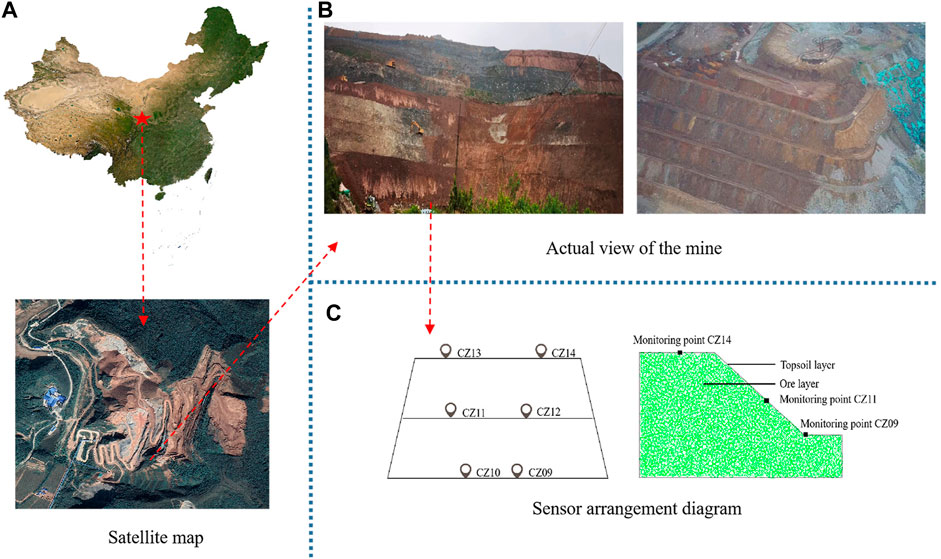
FIGURE 5. Mine location diagram and monitoring point layout chart.

The stability of rock slope is influenced by a variety of factors, which are mainly divided into four categories: engineering geology, geometric conditions, hydro-meteorology, and applied loads (as shown in Figure 6). Among them, rainfall is one of the critical factors affecting landslide deformation, and the changes in accumulated displacement of landslides and single-day precipitation during the monitoring period are shown in Figure 7. Temperature is one of the main factors affecting the mechanical properties of rocks (Li et al., 2022), and Weathering is the effect of changing the physical properties and chemical composition of rocks under atmospheric conditions. When other factors work together to a certain extent, it is very easy to cause slope instability, such as landslides, cave-ins, and other geological disasters, and rainfall, atmospheric radiation, temperature, and temperature difference are the main reasons affecting the weathering of rock slope. By geological survey of the mine site as well as its surrounding geology and literature query, the mine is divided into two segments, the left side of the western section is close to the Heng Shui River, and there is a tributary inflow, the size of the runoff from the Heng Shui River also affects the height of the groundwater level in the mine area, the rise and fall of the groundwater level cause the slope geotechnical body to produce deformation, slippage, collapse instability and other adverse geological phenomena, the groundwater level monitoring is mainly by means of pore water pressure sensors and stress gauges. Considering the above and the lag of some environmental impact factors on rock slope, the factors selected in this paper are daily rainfall (mm), accumulated rainfall (mm), daily average temperature (°C), daily temperature difference (°C), stress (Kpa), pore water pressure (Kpa), runoff (km), wind speed (m/s), among which the data of six factors such as rainfall, temperature, runoff and wind speed come from the meteorological monitoring station in Fengxiang District, Baoji City, Shaanxi Province. The stress and pore water pressure data comes from the measurement data of mine monitoring points.

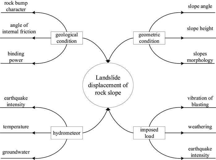
FIGURE 6. Diagram of influence factors of slope and landslide displacement.

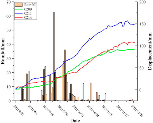
FIGURE 7. The changes of accumulated displacement of landslide and single-day precipitation during the monitoring period.

Influencing factors selection

Pearson correlation analysis was performed on the eight influencing factors, and their correlation coefficients were calculated (Figure 8). Taking the correlation analysis of impact factors of the monitoring point CZ11 as an example, The correlation coefficients between cumulative rainfall and pore water pressure, temperature and stress were 0.815, -884 and 0.658, respectively, while the correlation coefficients between runoff and pore water pressure were, 0.680 and between temperature and stress were -0.764, respectively. It shows a very high degree of correlation with a close relationship. In summarizing, all eight influence factors have a certain correlation with each other, which proves that there is redundancy among the data, and if the prediction is directly fused, the prediction performance of the prediction model will be affected to some extent. Therefore, this section calculated the correlation between each influence factor and landslide displacement using gray correlation analysis combined with the actual data from the experiment. The main influence factors were derived as the input variables of the prediction model (as shown in Table 2).

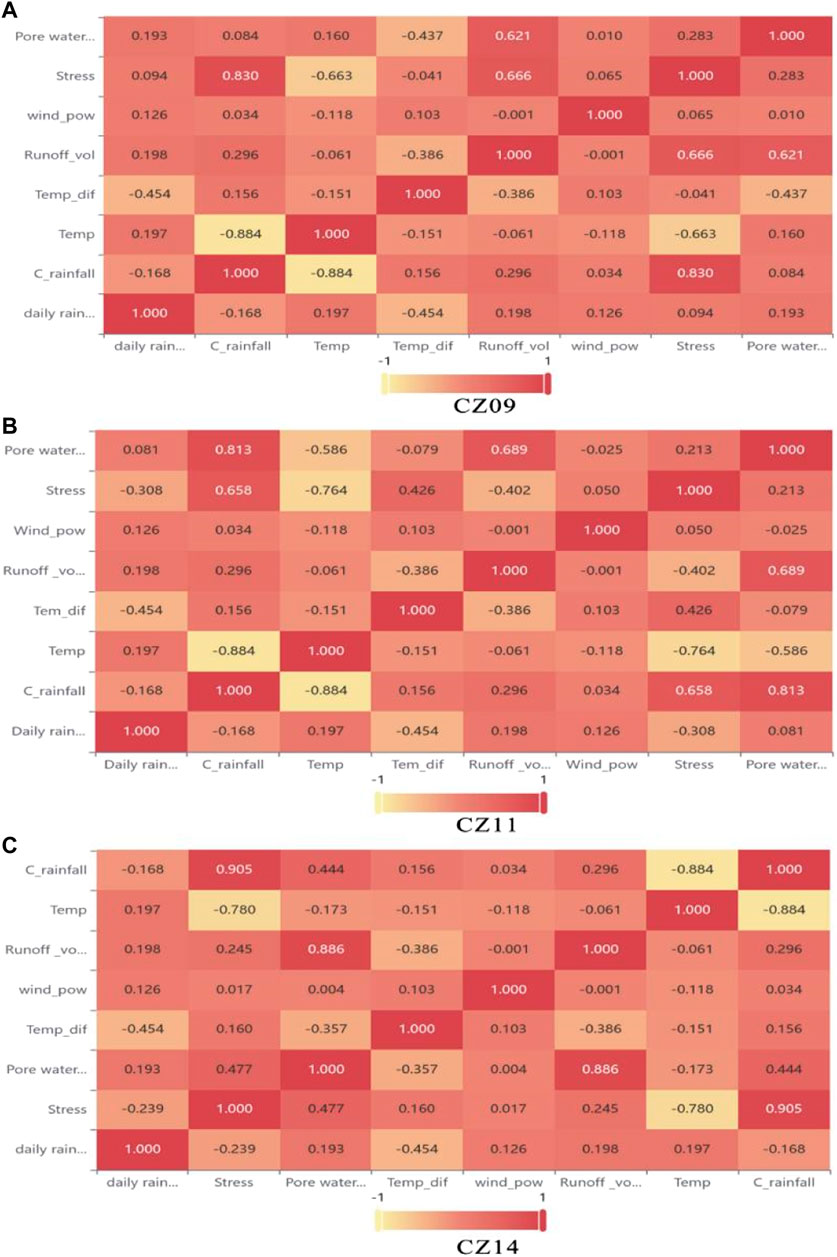
FIGURE 8. Correlation coefficient of three monitoring points influence factor (A) CZ09, (B) CZ11, (C) CZ14.

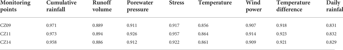
TABLE 2. The correlation between the influence factors of the three monitoring points and the displacement.

Taking monitoring point CZ11 as an example for analysis, combining Pearson correlation analysis and gray relational analysis for variable selection. Among the eight influencing factors, the top three correlations with landslide cumulative displacement are cumulative rainfall, stress, and pore water pressure, which are 0.973, 0.957, and 0.926, respectively. However, the correlation coefficients of cumulative rainfall and pore water pressure and stress are relatively large and strongly correlated. The two indicators of pore water pressure and stress are excluded, and the remaining six influencing factors are selected as input variables. Similarly, In monitoring points CZ09 and CZ14, the gray correlation between cumulative displacement and influence factors is greater for cumulative rainfall, stress, and temperature difference. However, since the correlation coefficients between cumulative rainfall and stress and temperature are higher, the two variables of stress and temperature are excluded, and the remaining six variables are retained as input variables.

Landslide displacement prediction

In the present study, the actual monitoring data of the Fengxiang cement mine from 25 August 2021, to 30 November 2021, are used as the experimental data, and there are 98 sets of valid data in total. As the slope has different responses to external influences at different locations, three sensors at different locations of the same slope will be selected for this experiment. The surface displacement data from each sensor will be predicted, the first 70 sets of data from each sensor will be selected as the training sample set, and the last 28 monitoring data will be used as the prediction sample set.

The parameters of the SSA-DELM method were set as follows: the population size of sparrows was 100; the proportion of discoverers was 0.7, and the proportion of vigilantes was 0.2; the hidden layer of the DELM model was set to 4 layers, the number of nodes in each implicit layer was set to 10, and the maximum number of iterations was 100; the excitation function was selected as sigmoid, and the excitation function was able to achieve nonlinear transformation in the feature space, and the SSA algorithm to optimize the implied layers and input thresholds of DELM. The convergence speed is shown in Figure 9, and it can be seen that the SSA-DELM model converges within 100 iterations, and the fitness values can all be maintained at about 1.2 × 10⁻³, indicating that the model converges quickly and has high prediction accuracy. The influence factors screened in the above section are used as input parameters and the accumulated displacement as output parameters.

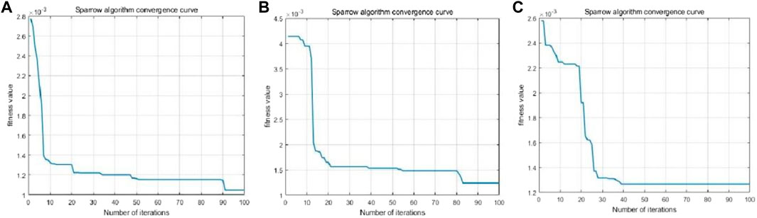
FIGURE 9. Data convergence speed graph for different measurement points, (A) CZ09, (B) CZ11, (C) CZ14.

As shown in Table 3, the displacement prediction errors at three different locations are relatively small by using the PCC-GRA-SSA-DELM prediction model, among which, the smallest RMSE and MAE is monitoring point CZ11 with RMSE of 1.44. From the plots (b) and (c) in Figure 10, it can be seen that the predicted displacement trends of monitoring point CZ11 and monitoring point CZ14 are the same as the actual displacement trends. Basically, the larger errors are in the first five groups of the test set. Besides, their actual values of them are lager than the predicted values. Accidental loads or human activities during the mining can cause this phenomenon. Monitoring point CZ09 has the largest RMSE and MAE, and the points with larger errors are basically located in the second half of the test set, which is attributed to the fact that monitoring point CZ09 is located at the foot of the slope, and the accidental displacements generated by mining activities and vehicle transportation will affect the accuracy of displacement prediction. In conclusion, the overall effect of the PCC-GRA-SSA-DELM prediction model is excellent and can be applied to the actual landslide displacement prediction.

TABLE 3. Error analysis table of 3 monitoring points.

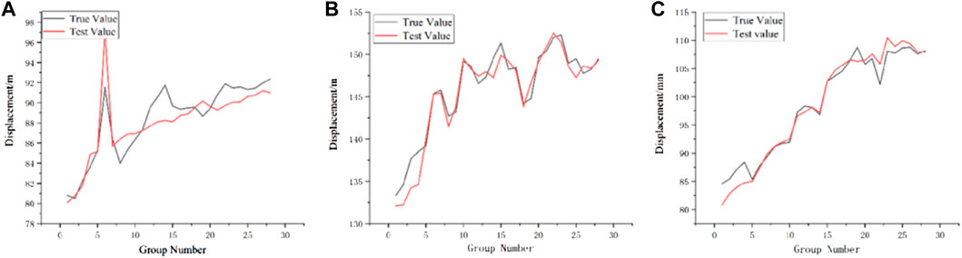
FIGURE 10. Comparison of predicted and actual values of three monitoring points, (A) CZ09, (B) CZ11, (C) CZ14.

Comparison verification

In order to verify the supremacy of the proposed model in this paper, a support vector machine (SVM), extreme learning machine (ELM), deep extreme learning machine (DELM), and SSA-DElM were built in Matlab to conduct comparison experiments with this paper’s model PCC-GRA-SSA-DELM (referred to as PGSD in the table) respectively. The prediction results of three different location sensors are shown in Table 4, among which the robustness of the ELM model is lowest.

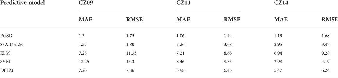
TABLE 4. Comparison of errors of different prediction models.

The comparison experiments use MAE and RMSE as evaluation indicators, where the smaller the two values are, the better their prediction. Among them, ELM has the lowest prediction accuracy compared with the other two derived algorithms, DELM and SSA-DELM. DELM has more ELM-AEs than ELM, which increases the stability and merit-seeking ability of the model. However, during the ELM-AE training process, the input layer weights and thresholds are randomly generated orthogonal random matrices in the DELM model. The ELM-AE unsupervised training process uses least squares to update the parameters. Only the output layer weights parameters are updated, while the input layer weights and thresholds are fixed. That means the prediction accuracy of DELM is affected by the random input weights and random thresholds of each ELM-AE. But the SSA can solve this problem. Therefore, SSA-DELM has the highest prediction accuracy. The PGSD model proposed in this paper reduces the dimensionality of input variables, removes strongly correlated variables, enhances of the relationship between input and output variables, avoids overfitting, and improves the overall model prediction accuracy. Compared to SSA-DELM, the results showed the accuracy by the PGSD model increased by 2.86, 60.8, and 51.59% at three different measurement points, respectively.

Conclusion

The present work combined variable selection and sparrow search algorithm-deep extreme learning machine algorithm to predict landslide displacement. The results were validated using monitoring data for a cement mine in Baoji City. The main findings of the study are summarized as follows:

1) The advantage of the variable selection is that it can remove redundancy between multi-variables and eliminate multicollinearity problems. The Pearson correlation analysis method identified the correlation coefficients between each variable. The magnitude of the correlation coefficients can be used to identify the redundancy between the variables. By combining with gray correlation analysis, the correlation between each input variable and the displacement can be calculated to eliminate the redundant variables and improve the accuracy of the prediction model.

2) The paper selected the locations of monitoring points at different locations of the same mine slope for the study. As a result, the correlation coefficients between landslide displacements and impact factors are different for different monitoring points, and the redundant and redundant variables to be eliminated are also different.

3) The PCC-GRA-SSA-DELM prediction model has a high predictive effect, and the overall effectiveness of fitting on three different monitoring points is strong, which can meet the demands of practical mine monitoring and early warning.

4) Compared with ELM, DELM and SVM traditional prediction algorithms, the PCC-GRA-SSA-DELM prediction model proposed in the research has higher prediction accuracy and prediction efficiency in rock slope landslide displacement prediction. Therefore, it is more suitable for the prediction of rock slope displacement.

In sum, the PCC-GRA-SSA-DELM fusion model proposed in this paper enriches the literature on the reliability of rock slope landslide monitoring and warning. The current research also has limits because the errors in original data caused by arbitrary factors, such as mining work, and human activities, are not considered. Therefore, future works can further focus on predicting periodic and trend term displacement by using the signal decomposition method to further enhance accuracy and reliability.

Data availability statement

The original contributions presented in the study are included in the article/Supplementary Material, further inquiries can be directed to the corresponding author.

Author contributions

SJ provided the ideas and framework for this study, including the methods and theories in the paper; HL, conducted the experiments and wrote this paper; ML, CL, and SZ, performed the preliminary reading of the first draft and gave critical comments; JL, assisted in the data processing and data analysis of this paper; PL, provided the test site and raw data, including the geographic location map of the mine, sensor data, etc. for this paper.

Funding

This work was supported by the research project of National Natural Science Foundation of China: Disaster identification and early warning of complex slope in open pit mine based on data knowledge hybrid drive (52104146); And the research project of Shaanxi Natural Science Foundation: Research on driverless vehicle road collaborative intelligent control system in open pit mine integrating 5G Technology (2021JQ-509); And Shaanxi Social Science Foundation: Research on intelligent comprehensive perception and disaster emergency decision-making of National Central Cities Based on big data (2020R005).

Conflict of interest

Author SJ was employed by the company Xi’an U-MINE Intelligent Mining Research Institute Co Ltd, Author ML was employed by the company Sinosteel Mining Development Co Ltd, and Author PL was employed by the company Jidong Cement Tongchuan Ltd.

The remaining authors declare that the research was conducted in the absence of any commercial or financial relationships that could be construed as a potential conflict of interest.

Publisher’s note

All claims expressed in this article are solely those of the authors and do not necessarily represent those of their affiliated organizations, or those of the publisher, the editors and the reviewers. Any product that may be evaluated in this article, or claim that may be made by its manufacturer, is not guaranteed or endorsed by the publisher.

Supplementary material

The Supplementary Material for this article can be found online at: https://www.frontiersin.org/articles/10.3389/fenvs.2022.982069/full#supplementary-material

References

Atzeni, C., Barla, M., Pieraccini, M., and Antolini, F (2015). Early warning monitoring of natural and engineered slopes with ground-based synthetic-aperture radar. Rock Mech. Rock Eng. 48, 235–246. doi:10.1007/s00603-014-0554-4
Chen, J., Zhu, C., Du, J. S., Pu, Y. Y., Pan, P. Z., Bai, J. B., et al. (2022). A quantitative pre-warning for coal burst hazard in a deep coal mine based on the spatio-temporal forecast of microseismic events. Process Saf. Environ. Prot. 159, 110. doi:10.1016/j.psep.2022.01.082
Du, Y., Li, H., Chicas, S. D., and Huo, L. C. (2022). Progress and perspectives of geotechnical anchor bolts on slope engineering in China. Front. Environ. Sci. 10. doi:10.3389/fenvs.2022.928064
Du, Y., Xie, M., and Jia, J. (2020). Stepped settlement: A possible mechanism for translational landslides. Catena 187, 104365. doi:10.1016/j.catena.2019.104365
Du, Y., Xie, M. W., Jiang, Y. J., Liu, W. N., Liu, R. C., and Liu, Q. Q. (2019). Research progress on dynamic monitoring index for early warning of rock collapse[J]. Chin. J. Eng. 41 (04), 427–435. doi:10.13374/j.issn2095-9389.2019.04.002
Duan, G. H., Niu, R. Q., Peng, L., and Fu, Jie. (2017). A landslide displacement prediction research based on optimizationparameter ARIMA model under the inducing factors[J]. Geomatics Inf. Sci. Wuhan Univ. 42 (04), 531–536. doi:10.13203/j.whugis20140913
Guo, Y. K., Zhang, S. A., Wang, J. J., Zhang, Q., and Xie, X. F. (2022). Feature variable selection combined with SVM for hyperspectral inversion of cultivated soil Hg content[J]. Eng. Surv. Mapp. 31 (01), 17–23. doi:10.19349/j.cnki.issn1006-7949.2022.01.003
Jiang, S., Li, J. Y., Zhang, S., Gu, Q. H., Lu, C. W., and Liu, H. S. (2022). Landslide risk prediction by using GBRT algorithm: Application of artificial intelligence in disaster prevention of energy mining. Process Saf. Environ. Prot. 166, 386. doi:10.1016/j.psep.2022.08.043
Jin, X. Z., Liu, Y., Yu, J., Wang, J. F., and Qie, Y. J. (2021). Prediction of outlet SO2 concentration based on variable selection and EMD-LSTM network[J]. Proc. CSEE 41 (24), 8475–8484. doi:10.13334/j.0258-8013.pcsee.202589
Li, B., Zhou, K., Ye, J., and Sha, P. (2019). Application of a probabilistic method based on neutrosophic number in rock slope stability assessment. Appl. Sci. (Basel). 9, 2309. doi:10.3390/app9112309
Li, H. W., Zhao, S. B., and Li, Z. (2021). Design and implementation of landslide early warning system based on multi-source monitoring data[J]. Sci-Tech Dev. Enterp. 2021 (12), 38–40. doi:10.3969/j.issn.1674-0688.2021.12.014
Li, P. X. (2021). Application of mutual information in feature selection algorithm[J]. Int. Core J. Eng. 7 (12), 0082. doi:10.6919/ICJE.202112_7(12).0082)
Li, X. S., Li, Q. H., Hu, Y. J., Chen, Q. S., Peng, J., Xie, Y. L., et al. (2021). Study on three-dimensional dynamic stability of open-pit high slope under blasting vibration [J]. Lithosphere 2021, 6426550. doi:10.2113/2022/6426550
Li, X. S., Peng, J., Xie, Y. L., Li, Q. H., Zhou, T., Wang, J. W., et al. (2022). Influence of high-temperature treatment on strength and failure behaviors of a quartz-rich sandstone under true triaxial condition [J]. Lithosphere 2022, 3086647. doi:10.2113/2022/3086647
Lian, X. G., Li, Z. J., Yuan, H. Y., Hu, H. F., Cai, Y. H., and Liu, X. Y. (2020). Determination of the stability of high-steep slopes by global navigation satellite system (GNSS) real-time monitoring in long wall mining. Appl. Sci. 10 (6), 1952. doi:10.3390/app10061952
Lin, X., Liu, Z. S., Gao, Y., and Wu, B. Y. (2019). Analysis of main controlling factors of oil production based on machine learning[J]. China CIO News 2019(12), 94–97+99. doi:10.3969/j.issn.1001-2362.2019.12.044
Liu, G., Ye, L. X., Chen, Q. Y., Chen, G. S., and Fan, M. Y. (2022). Abnormal event detection of city slope monitoring data based on multi-sensor information fusion[J]. Bull. Geol. Sci. Technol. 41 (02), 13–25. doi:10.19509/j.cnki.dzkq.2022.0060
Liu, W. Y., Men, D. Y., Liang, J. F., and Wang, W. Z. (2012). Monthly load forecasting based on gray relational degree and least squares support vector machine[J]. Power Syst. Technol. 36 (08), 228–232. doi:10.13335/j.1000-3673.pst.2012.08.036
Liu, Y., Xu, C., Huang, B., Ren, X. W., Liu, C. Q., Hu, B. D., et al. (2020). Landslide displacement prediction based on multi-source data fusion and sensitivity states. Eng. Geol. 271, 105608. doi:10.1016/j.enggeo.2020.105608
Liu, Z. B., Shao, J. F., Xu, W. Y., Chen, H. J., and Zhang, Y. (2014). An extreme learning machine approach for slope stability evaluation and prediction. Nat. Hazards (Dordr). 73 (2), 787–804. doi:10.1007/s11069-014-1106-7
Liu, Z. X., Han, K. W., Yang, S., and Liu, Y. X. (2020). Fractal evolution mechanism of rock fracture in undersea metal mining. J. Cent. South Univ. 27, 1320–1333. doi:10.1007/s11771-020-4369-z
Ma, K., Tang, C. A., Liang, Z. Z., Zhuang, D. Y., and Zhang, Q. B. (2017). Stability analysis and reinforcement evaluation of high-steep rock slope by microseismic monitoring. Eng. Geol. 218, 22–38. doi:10.1016/j.enggeo.2016.12.020
Meng, Q. X., Wang, J., Tao, Z. G., Ren, D. Z., Zhang, G. C., Li, X. S., et al. (2021) 3D nonlinear analysis of stilling basin in complex fractured dam foundation, Lithosphere 2021. 2738130. doi:10.2113/2022/2738130
Pang, J. (2019). Application of automatic monitoring system in high-risk slope monitoring project[J]. Surv. World 2019, 70–73. doi:10.3969/j.issn.1673-7563.2019.02.019
Peng, M., Li, X. Y., Li, D. Q., Jiang, S. H., and Zhang, L. M. (2014). Slope safety evaluation by integrating multi-source monitoring information. Struct. Saf. 49, 65–74. doi:10.1016/j.strusafe.2013.08.007
Pieraccini, M., Luzi, G., Mecatti, D., Noferini, L., and Atzeni, C. (2006). Ground-based SAR for short and long term monitoring of unstable slopes. IEEE 2006, 92–95. doi:10.1109/EURAD.2006.280281
Qin, H. N., Ma, H., N., and Yu, Z. X. (2020). Analysis method of landslide early warning and prediction supported by ground-based SAR technology[J]. Geomatics Inf. Sci. Wuhan Univer-sity 45 (11), 1697–1706. doi:10.13203/j.whugis20200268
Sakellariou, M. G., and Ferentinou, M. D. (2005). A study of slope stability prediction using neural networks. Geotech. Geol. Eng. (Dordr). 23, 419–445. doi:10.1007/s10706-004-8680-5
Salvoni, M., and Dight, P. M. (2016). Rock damage assessment in a large unstable slope from microseismic monitoring - MMG Century mine (Queensland, Australia) case study. Eng. Geol. 210, 45–56. doi:10.1016/j.enggeo.2016.06.002
Šegina, E., Peterne, l. T., Urbančič, T., Realini, E., Zupan, M., Jez, J., et al. (2020). Monitoring surface displacement of a deep-seated landslide by a low-cost and near real-time GNSS system. Remote Sens. 12 (20), 3375. doi:10.3390/rs12203375
Sulandri, S., Basuki, A., and Bachtiar, F. A. (2021). Metode deteksi intrusi menggunakan algoritme extreme learning machine dengan correlation-based feature selection. J. Teknol. Inf. Dan. Ilmu Kompute 8 (1), 103–110. doi:10.25126/jtiik.0813358
Tuerxun, M., Zhao, M. J., Ning, C. B., and Kong, Q. H. (2021). Prediction of diesel engine exhuast emissions based on deep extreme learning machine[J]. Sci. Technol. Eng. 21 (36), 15646–15654. doi:10.3969/j.issn.1671-1815.2021.36.046
Wang, L., Xu, H., Shu, B., and Tian, Y. Q. (2021). A multi-source heterogeneous data fusion method for landslide monitoring with mutual information and IPSO-lstm neural network[J]. Geomatics Inf. Sci. Wuhan Univ. 46 (10), 1478–1488. doi:10.13203/j.whugis20210131
Wang, R. B., Zhang, K., Qi, J., Xu, W. Y., Long, Y., and Huang, H. F. (2022). A prediction model of hydrodynamic landslide evolution process based on deep learning supported by monitoring big data. Front. Earth Sci. (Lausanne). 10, 15. doi:10.3389/feart.2022.829221
Wang, Z. W., Wang, L., Huang, G. W., Han, Q. Q., Xu, F., and Yue, C. (2020). Research on multi-source heterogeneous data fusion algorithm of landslide monitoring based on BP neural network [J]. J. Geomechanics 26, 575–582. doi:10.12090/j.issn.1006-6616.2020.26.04.050
Xu, B., Huang, Q. S., and Qian, Y. D. (2022). Stability trends of Jinpingzi landslide: Numerical study. Front. Earth Sci. 1465, 940438. doi:10.3389/feart.2022.940438
Xu, N. W., Li, B., Dai, F., Fang, Y. L., and Xu, J. (2016). Stability analysis of bedding rock slopes during excavation based on microseismic monitoring[J]. Chin. J. Rock Mech. Eng. 35 (10), 2089–2097. doi:10.13722/j.cnki.jrme.2015.0747
Xue, J., and Shen, B. (2020). A novel swarm intelligence optimization approach: Sparrow search algorithm. Syst. Sci. Control Eng. 8 (1), 22–34. doi:10.1080/21642583.2019.1708830
Yan, Y., Xiong, G. L., Zhou, J. J., Wang, R. H., Huang, R. H., Yang, M. W., et al. (2022). A whole process risk management system for the monitoring and early warning of slope hazards affecting gas and oil pipelines. Front. Earth Sci. (Lausanne). 9, 1336. doi:10.3389/feart.2021.812527
Yi, T., Han, X., Weitao, Y., Wenbing, G., Erhu, B., Tingye, Q., et al. (2022). Study on the overburden failure law of high-intensity mining in gully areas with exposed bedrock. Front. Earth Sci. 10, 833384. doi:10.3389/feart.2022.833384
Zeng, L., Lei, S. M., Wang, S. S., and Chang, Y. F. (2021). Ultra-short-term wind power prediction based on OVMD-SSA-DELM-GM model[J]. Power Syst. Technol. 45 (12), 4701–4712. doi:10.13335/j.1000-3673.pst.2021.0552
Zhang, L. F., Chen, Z. H., Zhou, T. B., Nian, G., Q., Wang, J., M., and Zhou, Z., H. (2020). Multi-source information fusion and stablity prediction of slope based on gradient boosting decision tree[J]. J. China Coal Soc. 45 (S1), 173–180. doi:10.13225/j.cnki.jccs.2020.0137
Zhang, Y. G., Tang, J., Cheng, Y. M., Huang, L., Guo, F., Yin, X. J., et al. (2022). Prediction of landslide displacement with dynamic features using intelligent approaches. Int. J. Min. Sci. Technol. 32, 539–549. doi:10.1016/j.ijmst.2022.02.004
Zhang, Y. H., Wang, Li., Shu, B., Haibo, H., and Long, L. (2020). “Application of an adaptive weighted estimation fusion algorithm in landslide deformation monitoring data processing,” in IOP Conference Series:Earth and Environmental Science, Changchun, China, 21-23 August 2020.
Keywords: multi-source data fusion, displacement prediction, SSA algorithm, deep extreme learning machine, variable selection
Citation: Jiang S, Liu H, Lian M, Lu C, Zhang S, Li J and Li P (2022) Rock slope displacement prediction based on multi-source information fusion and SSA-DELM model. Front. Environ. Sci. 10:982069. doi: 10.3389/fenvs.2022.982069
Received: 30 June 2022; Accepted: 24 August 2022;
Published: 28 September 2022.
Edited by:
Yan Du, University of Science and Technology Beijing, ChinaReviewed by:
Qiang Guo, China Jiliang University, ChinaBaiyu Chen, University of California, Berkeley, United States
Copyright © 2022 Jiang, Liu, Lian, Lu, Zhang, Li and Li. This is an open-access article distributed under the terms of the Creative Commons Attribution License (CC BY). The use, distribution or reproduction in other forums is permitted, provided the original author(s) and the copyright owner(s) are credited and that the original publication in this journal is cited, in accordance with accepted academic practice. No use, distribution or reproduction is permitted which does not comply with these terms.
*Correspondence: Hongsheng Liu, 1769303449@qq.com