Difference of anisotropic and isotropic TV for segmentation under blur and Poisson noise
 Kevin Bui
 Yifei Lou
 Fredrick Park
 Jack Xin
- 1Department of Mathematics, University of California, Irvine, Irvine, CA, United States
- 2Department of Mathematical Sciences, University of Texas at Dallas, Richardson, TX, United States
- 3Department of Mathematics & Computer Science, Whittier College, Whittier, CA, United States
In this paper, we aim to segment an image degraded by blur and Poisson noise. We adopt a smoothing-and-thresholding (SaT) segmentation framework that finds a piecewise-smooth solution, followed by k-means clustering to segment the image. Specifically for the image smoothing step, we replace the least-squares fidelity for Gaussian noise in the Mumford-Shah model with a maximum posterior (MAP) term to deal with Poisson noise and we incorporate the weighted difference of anisotropic and isotropic total variation (AITV) as a regularization to promote the sparsity of image gradients. For such a nonconvex model, we develop a specific splitting scheme and utilize a proximal operator to apply the alternating direction method of multipliers (ADMM). Convergence analysis is provided to validate the efficacy of the ADMM scheme. Numerical experiments on various segmentation scenarios (grayscale/color and multiphase) showcase that our proposed method outperforms a number of segmentation methods, including the original SaT.
1. Introduction
Image segmentation partitions an image into multiple, coherent regions, where pixels of one region share similar characteristics such as colors, textures, and edges. It remains an important yet challenging problem in computer vision that has various applications, including magnetic resonance imaging (Duan et al., 2015; Tongbram et al., 2021; Li et al., 2022) and microscopy (Zosso et al., 2017; Bui et al., 2020). One of the most fundamental models for image segmentation is the Mumford-Shah model (Mumford and Shah, 1989) because of its robustness to noise. Given an input image f : Ω → ℝ defined on an open, bounded, and connected domain Ω ⊂ ℝ2, the Mumford-Shah model is formulated as
where u : Ω → ℝ is a piecewise-smooth approximation of the image f, Γ ⊂ Ω is a compact curve representing the region boundaries, and λ, μ > 0 are the weight parameters. The first term in (1) is the fidelity term that ensures that the solution u approximates the image f. The second term enforces u to be piecewise smooth on Ω\Γ. The last term measures the perimeter, or more mathematically the one-dimensional Haussdorf measure in ℝ2 (Bar et al., 2011), of the curve Γ. However, (1) is difficult to solve because the unknown set of boundaries needs to be discretized. One common approach involves approximating the objective function in (1) by a sequence of elliptic functionals (Ambrosio and Tortorelli, 1990).
Alternatively, Chan and Vese (2001) (CV) simplified (1) by assuming the solution u to be piecewise constant with two phases or regions, thereby making the model easier to solve via the level-set method (Osher and Sethian, 1988). Let the level-set function ϕ be Lipschitz continuous and be defined as follows:
By the definition of ϕ, the curve Γ is represented by ϕ(x) = 0. The image region can be defined as either inside or outside the curve Γ. In short, the CV model is formulated as
where λ, ν are weight parameters, the constants c1, c2 are the mean intensity values of the two regions, and H(ϕ) is the Heaviside function defined by H(ϕ) = 1 if ϕ ≥ 0 and H(ϕ) = 0 otherwise. A convex relaxation (Chan et al., 2006) of (2) was formulated as
where an image segmentation ũ is obtained by thresholding u, that is
for some value τ ∈ (0, 1). It can be solved efficiently by convex optimization algorithms, such as the alternating direction method of multipliers (ADMM) (Boyd et al., 2011) and primal-dual hybrid gradient (Chambolle and Pock, 2011). A multiphase extension of (2) was proposed in Vese and Chan (2002), but it requires that the number of regions to be segmented is a power of 2. For segmenting into an arbitrary number of regions, fuzzy membership functions were incorporated (Li et al., 2010).
Cai et al. (2013) proposed the smoothing-and-thresholding (SaT) framework that is related to the model (1). In the smoothing step of SaT, a convex variant of (1) is formulated as
yielding a piecewise-smooth solution u*. The blurring operator A is included in the case when the image f is blurred. The total variation (TV) term is a convex approximation of the length term in (2) by the coarea formula (Chan et al., 2006). After the smoothing step, a thresholding step is applied to the smooth image u* to segment it into multiple regions. The two-stage framework has many advantages. First, the smoothing model (3) is strongly convex, so it can be solved by any convex optimization algorithm to obtain a unique solution u*. Second, the user can adjust the number of thresholds to segment u* and the threshold values to obtain a satisfactory segmentation result, thanks to the flexibility of the thresholding step. Furthermore, the SaT framework can be adapted to color images by incorporating an intermediate lifting step (Cai et al., 2017). Before performing the thresholding step, the lifting step converts the RGB space to Lab (perceived lightness, red- green and yellow-blue) color space and concatenates both RGB and Lab intensity values into a six-channel image. The multi-stage framework for color image segmentation is called smoothing, lifting, and thresholding (SLaT).
One limitation of (3) lies in the ℓ2 fidelity term that is statistically designed for images corrupted by additive Gaussian noise, and as a result, the smoothing step is not applicable to other types of noise distribution. In this paper, we aim at Poisson noise, which is commonly encountered when an image is taken by photon-capturing devices such as in positron emission tomography (Vardi et al., 1985) and astronomical imaging (Lantéri and Theys, 2005). By using the data fidelity term of Au − flogAu (Le et al., 2007), we obtain a smoothing model that is appropriate for Poisson noise (Chan et al., 2014):
As a convex approximation of the length term in (1), the TV term in (4) can be further improved by nonconvex regularizations. The TV regularization is defined by the ℓ1 norm of the image gradient. Literature has shown that nonconvex regularizations often yield better performance than the convex ℓ1 norm in identifying sparse solutions. Examples of nonconvex regularization include ℓp, 0 < p < 1 (Chartrand, 2007; Xu Z. et al., 2012; Cao et al., 2013), ℓ1 − αℓ2, α ∈ [0, 1] (Lou et al., 2015a,b; Ding and Han, 2019; Li P. et al., 2020; Ge and Li, 2021), ℓ1/ℓ2 (Rahimi et al., 2019; Wang et al., 2020; Xu et al., 2021), and an error function (Guo et al., 2021). Lou et al. (2015c) designed a TV version of ℓ1 − αℓ2 called the weighted difference of anisotropic–isotropic total variation (AITV), which outperforms TV in various imaging applications, such as image denoising (Lou et al., 2015c), image reconstruction (Lou et al., 2015c; Li P. et al., 2020), and image segmentation (Bui et al., 2021, 2022; Wu et al., 2022b).
In this paper, we propose an AITV variant of (4) to improve the smoothing step of the SaT/SLaT framework for images degraded by Poisson noise and/or blur. Incorporating AITV regularization is motivated by our previous works (Park et al., 2016; Bui et al., 2021, 2022), where we demonstrated that AITV regularization is effective in preserving edges and details, especially under Gaussian and impulsive noise. To maintain similar computational efficiency as the original SaT/SLaT framework, we propose an ADMM algorithm that utilizes the ℓ1 − αℓ2 proximal operator (Lou and Yan, 2018). The main contributions of this paper are as follows:
• We propose an AITV-regularized variant of (4) and prove the existence of a minimizer for the model.
• We develop a computationally efficient ADMM algorithm and provide its convergence analysis under certain conditions.
• We conduct numerical experiments on various grayscale/color images to demonstrate the effectiveness of the proposed approach.
The rest of the paper is organized as follows. Section 2 describes the background information such as notations, Poisson noise, and the SaT/SLaT framework. In Section 3, we propose a simplified Mumford-Shah model with AITV and a MAP data fidelity term for Poisson noise. In the same section, we show that the model has a global minimizer and develop an ADMM algorithm with convergence analysis. In Section 4, we evaluate the performance of the AITV Poisson SaT/SLaT framework on various grayscale and color images. Lastly, we conclude the paper in Section 5.
2. Preliminaries
2.1. Notation
Throughout the rest of the paper, we represent images and mathematical models in discrete notations (i.e., vectors and matrices). An image is represented as an M × N matrix, and hence the image domain is denoted by Ω = {1, 2, …, M} × {1, 2, …, N}. We define two inner product spaces: X: = ℝM×N and Y: = X × X. Let u ∈ X. For shorthand notation, we define u ≥ 0 if ui,j ≥ 0 for all (i,j) ∈ Ω. The discrete gradient operator ∇:X→Y is defined by (∇u)i, j = [(∇xu)i, j, (∇yu)i, j], where
and
The space X is equipped with the standard inner product 〈·, ·〉X, and Euclidean norm ||·||2. The space Y has the following inner product and norms: for p = (p1, p2) ∈ Y and q = (q1, q2) ∈ Y,
For brevity, we omit the subscript X or Y in the inner product when its context is clear.
2.2. AITV regularization
There are two popular discretizations of total variation: the isotropic TV (Rudin et al., 1992) and the anisotropic TV (Choksi et al., 2011), which are defined by
respectively. This work is based on the weighted difference between anisotropic and isotropic TV (AITV) regularization (Lou et al., 2015c), defined by
for a weighting parameter α ∈ [0, 1]. The range of α ensures the non-negativity of the AITV regularization. Note that anisotropic TV is defined as the ℓ1 norm of the image gradient [(∇xu)i,j, (∇yu)i,j] at the pixel location (i, j) ∈ Ω, while isotropic TV is the ℓ2 norm on the gradient vector. As a result, AITV can be viewed as the ℓ1 − αℓ2 regularization on the gradient vector at every pixel, thereby enforcing sparsity individually at each gradient vector.
2.3. Poisson noise
Poisson noise follows the Poisson distribution with mean and variance η, whose probability mass function is given by
For a clean image g ∈ X, its intensity value at each pixel gi, j serves as the mean and variance for the corresponding noisy observation f ∈ X defined by
To recover the image g from the noisy image f, we find its maximum a posteriori (MAP) estimation u, which maximizes the probability ℙ(u|f). By Bayes' theorem, we have
It further follows from the definition (6) that
Since Poisson noise is i.i.d. pixelwise, we have
The MAP estimate of ℙ(u|f) is equivalent to its negative logarithm, thus leading to the following optimization problem:
The last term −log ℙ(ui,j) can be regarded as an image prior or a regularization. For example, Le et al. (2007) considered the isotropic total variation as the image prior and proposed a Poisson denoising model
where log is applied pixelwise and 11 is the matrix whose entries are all 1's. The first term in (8) is a concise notation that is commonly used as a fidelity term for Poisson denoising in various imaging applications (Le et al., 2007; Chan et al., 2014; Wen et al., 2016; Chang et al., 2018; Chowdhury et al., 2020a,b).
2.4. Review of Poisson SaT/SLaT
A Poisson SaT framework (Chan et al., 2014) consists of two steps. Given a noisy grayscale image f ∈ X corrupted by Poisson noise, the first step is the smoothing step that finds a piecewise-smooth solution u* from the optimization model:
Then in the thresholding step, K − 1 threshold values τ1 ≤ τ2 ≤ … ≤ τK−1 are appropriately chosen to segment u* into K regions, where the kth region is given by
with . The thresholding step is typically performed by k-means clustering.
The Poisson smoothing, lifting, and thresholding (SLaT) framework (Cai et al., 2017) extends the Poisson SaT framework to color images. For a color image f = (f1, f2, f3) ∈ X × X × X, the model (9) is applied to each color channel fi for i = 1, 2, 3, thus leading to a smoothed color image . An additional lifting step (Luong, 1993) is performed to transform u* to in the Lab space (perceived lightness, red-green, and yellow-blue). The channels in Lab space are less correlated than in RGB space, so they may have useful information for segmentation. The RGB image and the Lab image are concatenated to form the multichannel image û: = , followed by the thresholding stage. Generally, k-means clustering yields K centroids c1, …, cK as constant vectors, which are used to form the region
for k = 1, …, K such that Ωk's are disjoint and .
After the thresholding step for both SaT/SLaT, we define a piecewise-constant approximation of the image f by
where ck, ℓ is the ℓth entry of the constant vector ck and
Recall that d = 1 when f is grayscale, and d = 3 when f is color.
3. Proposed approach
To improve the Poisson SaT/SLaT framework, we propose to replace the isotropic TV in (9) with AITV regularization. In other words, in the smoothing step, we obtain the smoothed image u* from the optimization problem
for α ∈ [0, 1]. We establish that this model admits a global solution. We then develop an ADMM algorithm to find a solution and provide the convergence analysis. The overall segmentation approach is described in Algorithm 1.
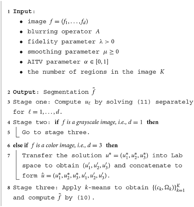
Algorithm 1. AITV Poisson SaT/SLaT.
3.1. Model analysis
To establish the solution's existence of the proposed model (11), we start with Lemma 1, a discrete version of Poincaré's inequality (Evans, 2010). In addition, we prove Lemma 2 and Proposition 3, leading to the global existence theorem (Theorem 4).
Lemma 1. There exists a constant C > 0 such that
for every u ∈ X and .
Proof. We prove it by contradiction. Suppose there exists a sequence such that
where . For every k, we normalize each element in the sequence by It is straightforward that
By (13), we have
As is bounded, there exists a convergent subsequence such that for v* ∈ X. It follows from (15) that Since ker(∇) = {c11:c ∈ ℝ}, then v* is a constant vector. However, (14) implies that and . This contradiction proves the lemma. ⃣
Lemma 2. Suppose ||f||∞ < ∞ and . There exists a scalar u0 > 0 such that we have 2(x − fi,j log x) ≥ x for any x ≥ u0 and (i, j) ∈ Ω.
Proof. For each (i,j) ∈ Ω, we want to show that there exists ui,j > 0 such that H(x): = x − 2fi,j log x ≥ 0 for x ≥ ui,j. Since H(x) is strictly convex and it attains a global minimum at x = 2fi,j, it is increasing on the domain x > 2fi,j. Additionally as x dominates log (x) as x → +∞, there exists ui,j > 2fi,j > 0 such that which implies that H(ui,j) = ui,j − 2fi,j log ui,j ≥ 0. As a result, for x ≥ ui,j > 2fi,j, we obtain x − 2fi,j log x = H(x) ≥ H(ui,j) ≥ 0. Define , and hence we have 2(x − fi,j log x) ≥ x for x ≥ u0 ≥ ui,j, ∀(i, j) ∈ Ω.
Proposition 3. Suppose ker(A) ∩ ker(∇) = {0} and . If is bounded, then is bounded.
Proof. Since ker(A) ∩ ker(∇) = {0}, we have A11 ≠ 0. Simple calculations lead to
where the last inequality is due to Lemma 1. The boundedness of and implies that is also bounded by (16). We apply Lemma 1 to obtain
which thereby proves that is bounded.
Finally, we adapt the proof in Chan et al. (2014) to establish that F has a global minimizer.
Theorem 4. Suppose ||f||∞ < ∞ and . If λ > 0, μ ≥ 0, α ∈ [0, 1), and ker(A) ∩ ker(∇) = {0}, then F has a global minimizer.
Proof. It is straightforward that ||∇u||2, 1 ≤ ||∇u||1, thus ||∇u||1 − α||∇u||2, 1 ≥ 0 for α ∈ [0, 1). As a result, we have
Given a scalar f > 0, the function G(x) = x − flog(x) attains its global minimum at x = f. Therefore, we have x − fi,j log x ≥ fi,j − fi,j log fi,j for all x > 0 and (i,j) ∈ Ω, which leads to a lower bound of F(u), i.e.,
As F(u) is lower bounded by F0, we can choose a minimizing sequence and hence F(uk) has a uniform upper bound, denoted by B1, i.e., F(uk) < B1 for all k ∈ ℕ. It further follows from (17) that
which implies that is uniformly bounded, i.e., there exists a constant B2 > 0 such that |〈Auk − f log Auk, 11〉| < B2, ∀k. Using these uniform bounds, we derive that
As α < 1, the sequence is bounded.
To prove the boundedness of , we introduce the notations of x+ = max(x, 0) and x− = −min(x, 0) for any x ∈ ℝ. Then x = x+ − x−. By Lemma 2, there exists u0 > 0 such that 2(x − fi,j log x) ≥ x, ∀x ≥ u0 and (i,j) ∈ Ω. We observe that
This shows that is bounded.
Since both and are bounded, then is bounded due to Proposition 3. Therefore, there exists a subsequence that converges to some u* ∈ X. As F is continuous and thus lower semicontinuous, we have
which means that u* minimizes F.
3.2. Numerical algorithm
To minimize (11), we introduce two auxiliary variables v ∈ X and w = (wx, wy) ∈ Y, leading to an equivalent constrained optimization problem:
The corresponding augmented Lagrangian is expressed as
where y ∈ X and z = (zx, zy) ∈ Y are Lagrange multipliers and β1, β2 are positive parameters. We then apply the alternating direction method of multipliers (ADMM) to minimize (19) that consists of the following steps per iteration k:
where σ > 1.
Remark 1. The scheme presented in (21) slightly differs from the original ADMM (Boyd et al., 2011), the latter of which has σ = 1 in (21f). Having σ > 1 increases the weights of the penalty parameters β1, k, β2, k in each iteration k, thus accelerating the numerical convergence speed of the proposed ADMM algorithm. A similar technique has been used in Cascarano et al. (2021), Gu et al. (2017), Storath and Weinmann (2014), Storath et al. (2014), and You et al. (2019).
All the subproblems (21a)–(21c) have closed-form solutions. In particular, the first-order optimality condition for (21a) is
where Δ = −∇⊤∇ is the Laplacian operator. If ker(A) ∩ ker(∇) = {0}, then is positive definite and thereby invertible, which implies that (22) has a unique solution uk+1. By assuming periodic boundary condition for u, the operators Δ and A⊤A are block circulant (Wang et al., 2008), and hence (22) can be solved efficiently by the 2D discrete Fourier transform . Specifically, we have the formula
where is the inverse discrete Fourier transform, the superscript * denotes complex conjugate, the operation ° is componentwise multiplication, and division is componentwise. By differentiating the objective function of (21b) and setting it to zero, we can get a closed-form solution for vk+1 given by
where the square root, squaring, and division are performed componentwise. Lastly, the w-subproblem (21c) can be decomposed componentwise as follows:
where the proximal operator for ℓ1 − αℓ2 on x ∈ ℝn is given by
The proximal operator for ℓ1 − αℓ2 has a closed form solution summarized by Lemma 5.
Lemma 5. (Lou and Yan, 2018) Given x ∈ ℝn, β > 0, and α ∈ [0, 1], the optimal solution to (26) is given by one of the following cases:
1. When ||x||∞ > β, we have
where ξ = sign(x)° max (|x| − β, 0).
2. When (1 − α)β < ||x||∞ ≤ β, then x* is a 1-sparse vector such that one chooses i ∈ argmaxj(|xj|) and defines and the remaining elements equal to 0.
3. When ||x||∞ ≤ (1 − α)β, then x* = 0.
In summary, we describe the ADMM scheme to solve (11) in Algorithm 2.
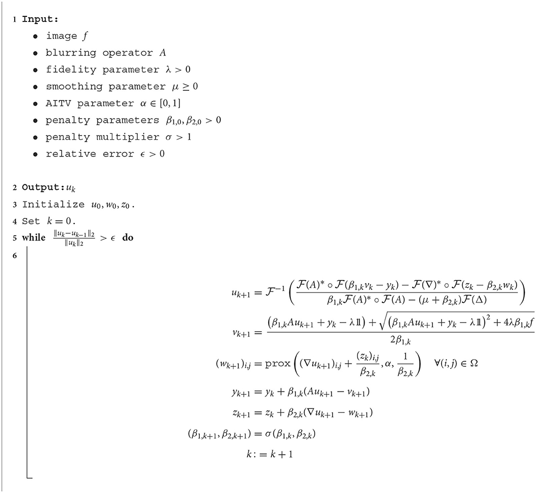
Algorithm 2. ADMM for the AITV-regularized smoothing model with Poisson fidelity (Equation 11).
3.3. Convergence analysis
We establish the subsequential convergence of ADMM described in Algorithm 2. The global convergence of ADMM (Wang et al., 2019) is inapplicable to our model as the gradient operator ∇ is non-surjective, which will be further investigated in future work. For the sake of brevity, we set β = β1 = β2 and denote
In addition, we introduce definitions of subdifferentials (Rockafellar and Wets, 2009), which defines a stationary point of a non-smooth objective function.
Definition 6. For a proper function h:ℝn → ℝ∪{+∞}, define dom(h): = {x ∈ ℝn:h(x) < +∞}.
(a) The regular subdifferential at x ∈ dom(h) is given by
(b) The (limiting) subdifferential at x ∈ dom(h) is given by
An important property of the limiting subdifferential is its closedness: for any (xk, vk) → (x, v) with vk ∈ ∂h(xk), if h(xk) → h(x), then v ∈ ∂h(x).
Lemma 7. Suppose that ker(A) ∩ ker(∇) = {0} and 0 ≤ α < 1. Let be a sequence generated by Algorithm 2. Then, we have
for some constant ν > 0.
Proof. If ker(A) ∩ ker(∇) = {0}, then is positive definite, and hence there exists ν > 0 such that
which implies that is strongly convex with respect to u with parameter ν. Additionally, is strongly convex with respect to v with parameter β0 ≤ βk. It follows from Beck (2017), Theorem 5.25, that we have
As wk+1 is the optimal solution to (21c), it is straightforward to have
Simple calculations by using (21d)–(21e) lead to
Lastly, we have
Combining (29)–(33) together with the fact that for σ > 1, we obtain
This completes the proof.
Lemma 8. Suppose that ker(A) ∩ ker(∇) = {0} and 0 ≤ α < 1. Let be generated by Algorithm 2. If bounded, then the sequence is bounded, uk+1−uk → 0, and vk+1−vk → 0.
Proof. First we show that is bounded. Combining (21e) with the first-order optimality condition of (25), we have
which implies that there exist ξ1 ∈ ∂||(wk+1)i,j||1 and ξ2 ∈ ∂||(wk+1)i,j||2 such that (zk+1)i,j = ξ1−αξ2 for each (i,j) ∈ Ω. Recall that for x ∈ ℝ2 the subgradients of the two norms are
Therefore, we have ||ξ1||∞ ≤ 1, ||ξ2||∞ ≤ 1, and hence ||(zk+1)i,j||∞ ≤ 1+α (by the triangle inequality), i.e., is bounded.
By the assumption is bounded. There exist two constants C1, C2 > 0 such that , , , and for all k ∈ ℕ. Hence, we have from (28) that
A telescoping summation of (37) leads to
By completing two least-squares terms, we can rewrite as
Combining (38) and (39), we have
Since σ > 1, the infinite sum is finite, and hence we have ∀k ∈ ℕ,
which implies that is bounded. Also from (38) and (39), we have
This shows that is bounded. By emulating the computation in (18), it can be shown that is bounded.
It suffices to prove that is bounded in order to prove the boundedness of by Proposition 3. Using (21d), we have
As is proven to be bounded, then is also bounded. We can prove is bounded similarly using (21e). Altogether, is bounded.
It follows from (40) that
As k → ∞, we see the right-hand side is finite, which forces the infinite summations on the left-hand side to converge, and hence we have uk+1 − uk → 0 and vk+1 − vk → 0.
Theorem 9. Suppose that ker(A) ∩ ker(∇) = {0} and 0 ≤ α < 1. Let be generated by Algorithm 2. If bounded, βk(vk+1 − vk) → 0, βk(wk+1 − wk) → 0, yk+1 − yk → 0, and zk+1 − zk → 0, then there exists a subsequence whose limit point (u*, v*, w*, y*, z*) is a stationary point of (19) that satisfies the following:
Proof. By Lemma 8, the sequence is bounded, so there exists a subsequence that converges to a point (u*, v*, w*, y*, z*). Additionally, we have uk+1 − uk → 0 and vk+1 − vk → 0. Since is bounded, there exists a constant C > 0 such that ||yk+1 − yk||2 < C and ||zk+1 − zk||2 < C for each k ∈ ℕ. By (21e), we have
As k → ∞, we have wk+1−wk → 0. Altogether, we can derive the following results:
Furthermore, the assumptions give us
By (21d)–(21e), we have
Hence, we have Au* = v* and ∇u* = w*.
The optimality conditions at iteration kn are the following:
Expanding (43a) by substituting in (21d)–(21e) and taking the limit, we have
Substituting in (21d) into (43b) and taking the limit give us
Lastly, by substituting (21e) into (43c), we have
By continuity, we have . Together with the fact that , we have by closedness of the subdifferential.
Therefore, (u*, v*, w*, y*, z*) is a stationary point.
Remark 2. It is true that the assumptions in Theorem 9 are rather strong, but they are standard in the convergence analyses of other ADMM algorithms for nonconvex problems that fail to satisfy the conditions for global convergence in Wang et al. (2019). For example, Jung (2017), Jung et al. (2014), Li et al. (2016) and Li Y. et al. (2020) assumed convergence of the successive differences of the primal variables and Lagrange multipliers. Instead, we modify the convergence of the successive difference of the primal variables, i.e., βk(vk+1 − vk) → 0, βk(wk+1 − wk) → 0. Boundedness of the Lagrange multiplier (i.e., ) was also assumed in Liu et al. (2022) and Xu Y. et al. (2012), which required a stronger assumption than ours regarding the successive difference of the Lagrange multipliers.
4. Numerical experiments
In this section, we apply the proposed method of AITV Poisson SaT/SLaT on various grayscale and color images for image segmentation. For grayscale images, we compare our method with the original TV SaT (Chan et al., 2014), thresholded-Rudin-Osher-Fatemi (T-ROF) (Cai et al., 2019), and the Potts model (Potts, 1952) solved by either Pock's algorithm (Pock) (Pock et al., 2009) or Storath and Weinmann's algorithm (Storath) (Storath and Weinmann, 2014). For color images, we compare with TV SLaT (Cai et al., 2017), Pock's method (Pock et al., 2009), and Storath's method (Storath and Weinmann, 2014). We can solve (9) for TV SaT/SLaT via Algorithm 2 that utilizes the proximal operator corresponding to the ||·||2, 1 norm. The code for T-ROF is provided by the respective author1 and we can adapt it to handle blur by using a more general data fidelity term. Pock's method is implemented by the lab group2. Storath's method is provided by the original author3. Note that T-ROF, Pock's method, and Storath's method are designed for images corrupted with Gaussian noise. We apply the Anscombe transform (Anscombe, 1948) to the test images, after which the Poisson noise becomes approximately Gaussian noise. Since Storath's method is not for segmentation, we perform a post-processing step of k-means clustering to its piecewise-constant output. For the SLaT methods, we parallelize the smoothing step separately for each channel.
To quantitatively measure the segmentation performance, we use the DICE index (Dice, 1945) and peak signal-to-noise ratio (PSNR). Let S ⊂ Ω be the ground-truth region and S′ ⊂ Ω be a region obtained from the segmentation algorithm corresponding to the ground-truth region S. The DICE index is formulated by
To compare the piecewise-constant reconstruction according to (10) with the original test image f, we compute PSNR by
where M × N is the image size and .
Poisson noise is added to the test images by the MATLAB command poissrnd. To ease parameter tuning, we scale each test image to [0, 1] after its degradation with Poisson noise and/or blur. We set σ = 1.25 and β1, 0 = β2, 0 = 1.0, 2.0 in Algorithm 2 for grayscale and color images, respectively. The stopping criterion is either 300 iterations or when the relative error of uk is below ϵ = 10−4. We tune the fidelity parameter λ and the smoothing parameter μ for each image, which will be specified later. For T-ROF, Pock's method, and Storath's method, their parameters are manually tuned to give the best DICE indices for binary segmentation (Section 4.1) and the PSNR values for multiphase segmentation (Sections 4.2-4.3). All experiments are performed in MATLAB R2022b on a Dell laptop with a 1.80 GHz Intel Core i7-8565U processor and 16.0 GB RAM.
4.1. Grayscale, binary segmentation
We start with performing binary segmentation on the entire DRIVE dataset (Staal et al., 2004) that consists of 20 images shown in Figure 1. Each image has size 584 × 565 with modified pixel values of either 200 for the background or 255 for the vessels. Before adding Poisson noise, we set the peak value of the image to be P/2 or P/5, where P = 255. Note that a lower peak value indicates stronger noise in the image, thus more challenging for denoising. We examine three cases: (1) P/2 no blur, (2) P/5 no blur, and (3) P/2 with Gaussian blur specified by MATLAB command fspecial(“gaussian,” [10 10], 2). For the TV SaT method, we set λ = 14.5, μ = 0.5 for case (1), λ = 8.0, μ = 0.5 for case (2), and λ = 22.5, μ = 0.25 for case (3). For the AITV SaT method, the parameters λ and μ are set the same as TV SaT, and we have α = 0.3 for cases (1)–(2) and α = 0.8 for case (3).
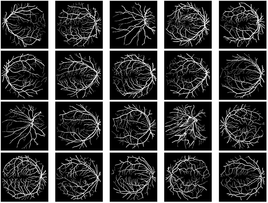
Figure 1. The entire DRIVE dataset (Staal et al., 2004) for binary segmentation. The image size is 584×565 with background value of 200 and the pixel value for vessels to be 255.
Table 1 records the DICE indices and the computational time in seconds for the competing methods, averaged over 20 images. We observe that AITV SaT attains the best DICE indices for all three cases with comparable computational time to TV SaT and T-ROF, all of which are much faster than Pock and Storath. As visually illustrated in Figure 2, AITV SaT segments more of the thinner vessels compared to TV SaT and T-ROF in five images, thereby having the higher average DICE indices.
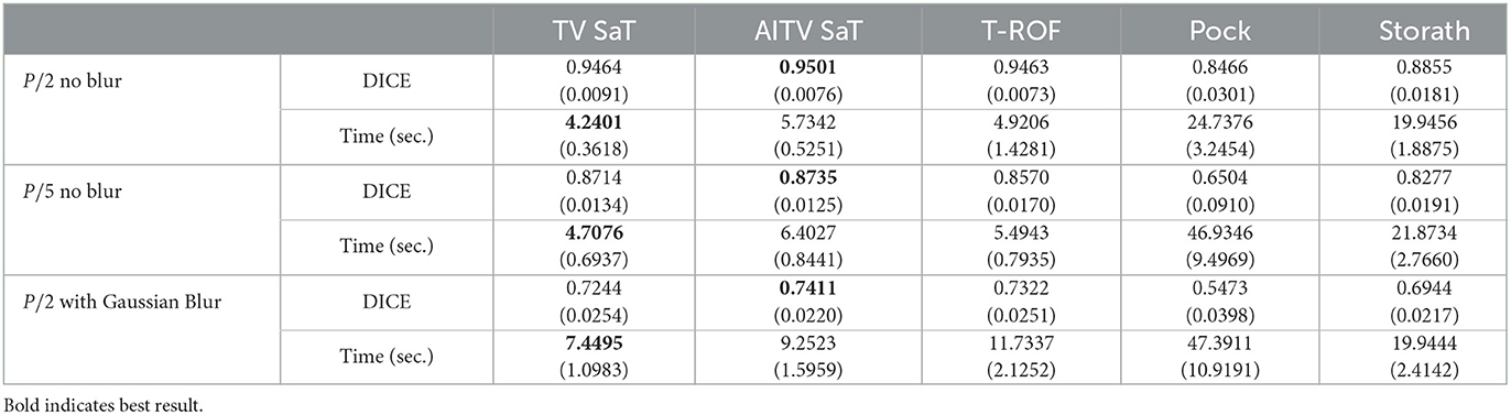
Table 1. DICE and computational time in seconds of the binary segmentation methods averaged over 20 images in Figure 1 with standard deviations in parentheses.
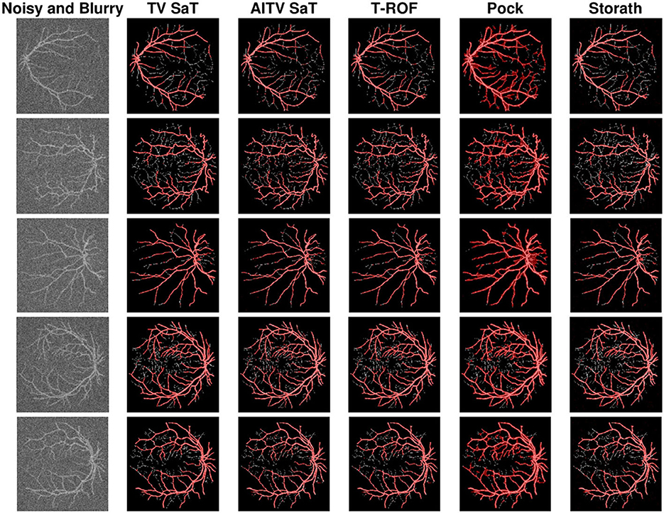
Figure 2. Binary segmentation results of Figure 1 with peak P/2 under Gaussian blur and Poisson noise.
4.2. Grayscale, multiphase segmentation
We examine the multiphase segmentation on the entire BrainWeb dataset (Aubert-Broche et al., 2006) that consists of 20 grayscale images as shown in Figure 3. Each image is of size 104 × 87 and has four regions to segment: background, cerebrospinal fluid (CSF), gray matter (GM), and white matter (WM). The pixel values are 10 (background), 48 (CSF), 106 (GM), and 154 (WM). The maximum intensity P = 154. We consider two cases: (1) P/2 no blur and (2) P/2 with motion blur specified by fspecial(“motion,” 5, 225). For the SaT methods, we have μ = 1.0, α = 0.6, 0.7, and λ = 4.0, 5.0 for case (1) and case (2), respectively.
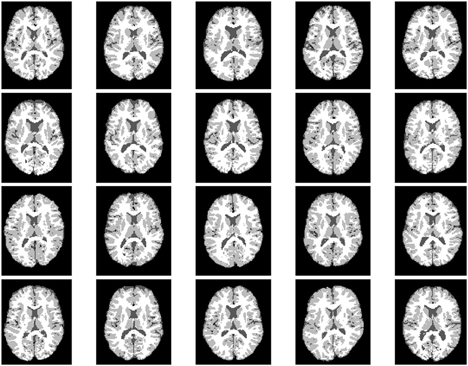
Figure 3. The entire BrainWeb dataset (Aubert-Broche et al., 2006) for grayscale, multiphase segmentation. Each image is of size 104 × 87. The pixel values are 10 (background), 48 (cerebrospinal fluid), 106 (gray matter), and 154 (white matter).
Across all 20 images of the BrainWeb dataset, Table 2 reports the average DICE indices for CSF, GM, and WM and average computational times in seconds of the segmentation methods. For both cases (1) and (2), AITV SaT attains the highest average DICE indices for segmenting CSF, GM, and WM. AITV SaT is comparable to TV SaT and T-ROF in terms of computational time.
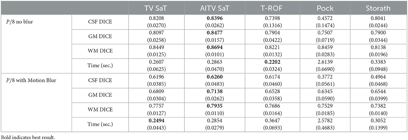
Table 2. DICE and computational time in seconds of the multiphase segmentation methods averaged over 20 images in Figure 3 with standard deviations in parentheses.
Figure 4 shows the segmentation results of the first image in Figure 3 for case (1). When segmenting CSF, the methods (TV SaT, AITV SaT, and Storath) yield similar visual results, while Pock fails to segment roughly half of the region. In addition, AITV SaT segments the most GM region with the least amount of noise artifacts than the other methods. Lastly, for WM segmentation, AITV SaT avoids the “holes” or “gaps” and segments fewer regions outside of the ground truth, thus outperforming TV SaT and Storath. For the three regions, T-ROF has the most noise artifacts in its segmentation results.
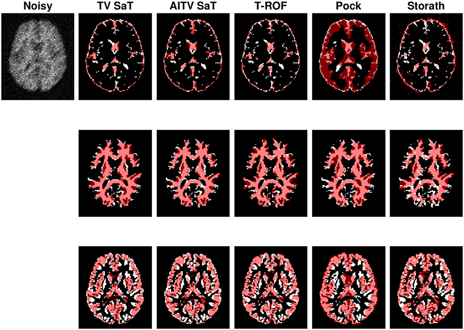
Figure 4. Segmentation result of the first image of Figure 3 with peak P/8 under Poisson noise with no blur. From top to bottom are segmentation results for CSF, GM, and WM.
4.3. Color segmentation
We perform color image segmentation on 10 images shown in Figure 5, which are selected from the PASCAL VOC 2010 dataset (Everingham et al., 2009). Each image has six different color regions. Figure 5A is of size 307 × 461; Figure 5B is of 500 × 367; Figures 5C, H, I are of 500 × 375; and Figures 5D–G, J are of 375 × 500. Before adding Poisson noise to each channel of each image, we set the peak value P = 10. We choose the parameters of the SLaT methods to be λ = 1.5, μ = 0.05, and α = 0.6.
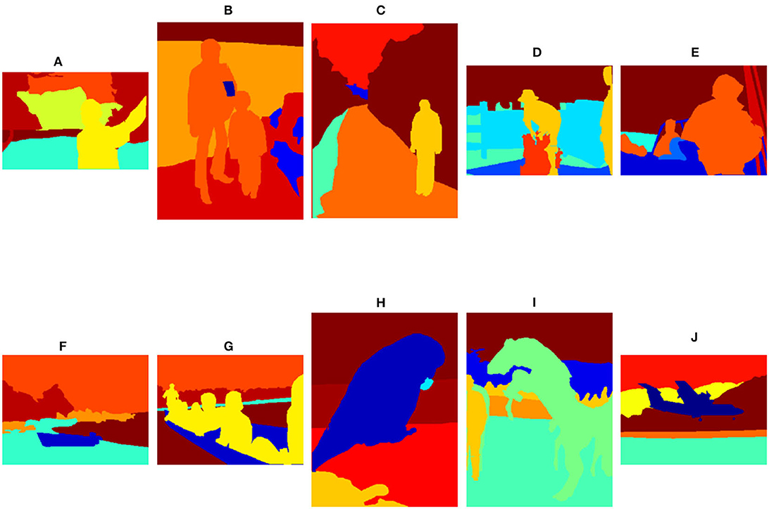
Figure 5. Test images from the PASCAL VOC 2010 dataset (Everingham et al., 2009) for color, multiphase segmentation. Each image has six regions. The image sizes are (A) 307 × 461, (B) 500 × 367, (C) 500 × 375, (D–G) 375 × 500, (H, I) 500 × 375, and (J) 375 × 500.
Figures 6, 7 present the piecewise-constant approximations via (10), showing similar segmentation results obtained by TV SLaT, AITV SLaT, and Storath. Quantitatively in Table 3, AITV SLaT has better PSNRs than TV SLaT and Pock for all the images and outperforms Storath for seven. Overall, the proposed AITV SLaT has the highest PSNR on average over 10 images with the lowest standard deviation and comparable speed as Storath.
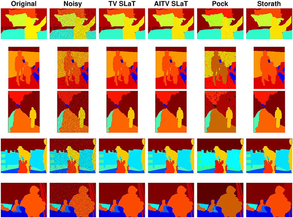
Figure 6. Color image segmentation results of Figures 5A–E.
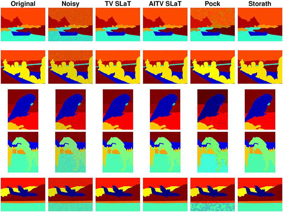
Figure 7. Color image segmentation results of Figures 5F–J.
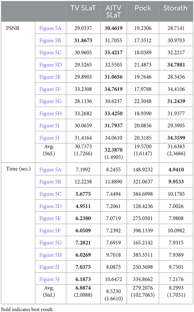
Table 3. PSNR and computation time in seconds for color image segmentation of the images in Figure 5.
4.4. Parameter analysis
The proposed smoothing model (11) involves the following parameters:
• The fidelity parameter λ weighs how close the approximation Au* is to the original image f. For a larger amount of noise, the value of λ should be chosen smaller.
• The smoothing parameter μ determines how smooth the solution u* should be. A larger value of μ may improve denoising, but at a cost of smearing out the edges between adjacent regions, which may be segmented together if they have similar colors.
• The sparsity parameter α ∈ [0, 1] determines how sparse the gradient vector at each pixel should be. More specifically, the closer the value α is to 1, the more ||∇u||1−α||∇u||2, 1 resembles ||∇u||0.
We perform sensitivity analysis on these parameters to understand how they affect the segmentation quality of AITV SaT/SLaT. We consider two types of tests in the case of P/8 with motion blur in Figure 3. In the first case (Figure 8), we fix μ = 1.0 and vary α, λ. In the second case (Figure 9), we fix λ = 5.0 and vary α, μ. Figure 8 reveals a concave relationship of the DICE index of each region with respect to the parameter λ, which implies there exists the optimal choice of λ. Additionally, when λ is small, a large value for α can improve the DICE indices. According to Figure 9, the DICE indices of the GM and WM regions decrease with respect to μ, while the DICE index of the CSF region is approximately constant. For α = 0.8, the DICE indices of the GM and WM regions are the largest when μ ≥ 1, but the large α is not optimal for CSF. Hence, an intermediate value of α, such as 0.6, is preferable to attain satisfactory segmentation quality for all three regions.
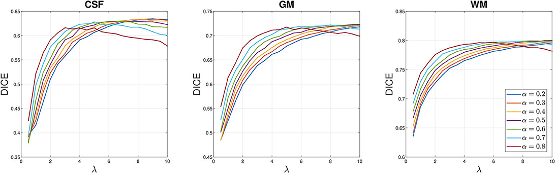
Figure 8. Sensitivity analysis on λ for the P/8 with motion blur case of Figure 3. The parameter μ = 1.0 is fixed. DICE indices averaged over 20 images for each brain region are plotted with respect to λ.
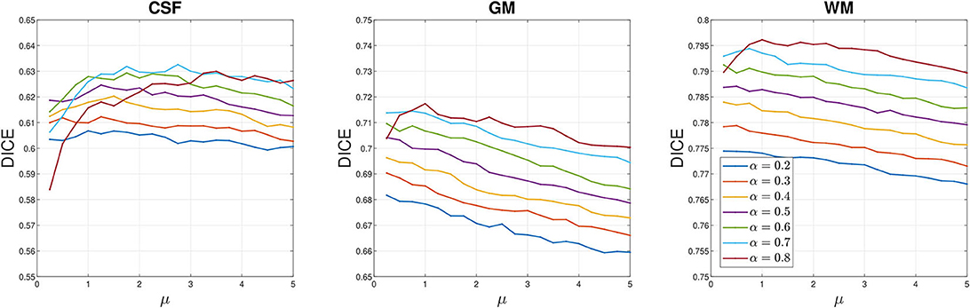
Figure 9. Sensitivity analysis on μ for the P/8 with motion blur case of Figure 3. The parameter λ = 5.0 is fixed. DICE indices averaged over 20 images for each brain region are plotted with respect to μ.
Lastly, in Figure 10, we conduct sensitive analysis for the case of P = 10 of Figure 5. We fix μ = 0.05, while varying λ, α in Figure 10A, which indicates that the optimal value for α is in the range of 0.5 ≤ α ≤ 0.7. Then we fix λ = 1.5 to examine μ and α in Figure 10B. For 0.2 ≤ α ≤ 0.7, PSNR decreases as μ increases. Again, α = 0.6 generally yields the best PSNR.
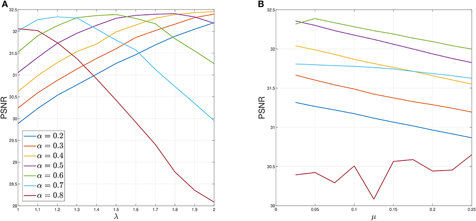
Figure 10. Sensitivity analysis of parameters for P = 10 case of Figure 5. (A) Sensitivity analysis on λ when μ = 0.05 fixed. (B) Sensitivity analysis on μ when λ = 1.5 fixed. Average PSNR is plotted.
5. Conclusion and future work
In this paper, we developed the AITV Poisson SaT/SLaT framework for image segmentation. In particular, we proposed a simplified Mumford-Shah model with the AITV regularization and Poisson fidelity for the smoothing step. The model was proven to have a global minimizer. Our numerical algorithm incorporated a specific splitting scheme for ADMM and the ℓ1−αℓ2 proximal operator for solving a subproblem. Convergence analysis established that the sequence generated by ADMM has a convergent subsequence to a stationary point of the nonconvex model. In our numerical experiments, the AITV Poisson SaT/SLaT yielded high-quality segmentation results within seconds for various grayscale and color images corrupted with Poisson noise and/or blur. For future directions, we are interested in other nonconvex regularization, such as ℓ1/ℓ2 on the gradient (Wang et al., 2021, 2022; Wu et al., 2022a), ℓp, 0 < p < 1, on the gradient (Hintermüller and Wu, 2013; Li Y. et al., 2020; Wu et al., 2021b), and transformed total variation (Huo et al., 2022), as alternatives to AITV. On the other hand, we can develop AITV variants of weighted TV (Li and Li, 2022) or adaptive TV (Wu et al., 2021a; Zhang et al., 2022). Moreover, we plan to determine how to make the sparsity parameter α in AITV adaptable to each image. In future work, we will adapt other segmentation algorithms (Li et al., 2010, 2016; Jung et al., 2014; Jung, 2017; Cai et al., 2019; Yang et al., 2022; Pang et al., 2023) designed for Gaussian noise or impulsive noise to Poisson noise.
Data availability statement
Publicly available datasets were analyzed in this study. This data can be found at: https://drive.grand-challenge.org/DRIVE/; https://github.com/casperdcl/brainweb; https://www2.eecs.berkeley.edu/Research/Projects/CS/vision/bsds/. Code for AITV Poisson SaT/SLaT is available at https://github.com/kbui1993/Official_Poisson_AITV_SaT_SLaT.
Author contributions
KB performed the experiments and analysis and drafted the manuscript. All authors contributed to the design, evaluation, discussions, and production of the manuscript. All authors contributed to the article and approved the submitted version.
Funding
This work was partially supported by NSF grants DMS-1846690, DMS-1854434, DMS-1952644, DMS-2151235, and a Qualcomm Faculty Award.
Conflict of interest
The authors declare that the research was conducted in the absence of any commercial or financial relationships that could be construed as a potential conflict of interest.
Publisher's note
All claims expressed in this article are solely those of the authors and do not necessarily represent those of their affiliated organizations, or those of the publisher, the editors and the reviewers. Any product that may be evaluated in this article, or claim that may be made by its manufacturer, is not guaranteed or endorsed by the publisher.
Footnotes
1. ^https://xiaohaocai.netlify.app/download/
2. ^Python code is available at https://github.com/VLOGroup/pgmo-lecture/blob/master/notebooks/tv-potts.ipynb and a translated MATLAB code is available at https://github.com/kbui1993/MATLAB_Potts.
References
Ambrosio, L., and Tortorelli, V. M. (1990). Approximation of functional depending on jumps by elliptic functional via t-convergence. Commun. Pure Appl. Math. 43, 999–1036. doi: 10.1002/cpa.3160430805
Anscombe, F. J. (1948). The transformation of Poisson, binomial and negative-binomial data. Biometrika 35, 246–254. doi: 10.1093/biomet/35.3-4.246
Aubert-Broche, B., Griffin, M., Pike, G. B., Evans, A. C., and Collins, D. L. (2006). Twenty new digital brain phantoms for creation of validation image data bases. IEEE Trans. Med. Imaging 25, 1410–1416. doi: 10.1109/TMI.2006.883453
Bar, L., Chan, T. F., Chung, G., Jung, M., Kiryati, N., Mohieddine, R., et al. (2011). “Mumford and Shah model and its applications to image segmentation and image restoration,” in Handbook of Mathematical Methods in Imaging, ed O. Scherzer (New York, NY: Springer), 1095–1157. doi: 10.1007/978-0-387-92920-0_25
Beck, A. (2017). First-order Methods in Optimization. Philadelphia, PA: SIAM. doi: 10.1137/1.9781611974997
Boyd, S., Parikh, N., Chu, E., Peleato, B., and Eckstein, J. (2011). Distributed optimization and statistical learning via the alternating direction method of multipliers. Found. Trends Mach. Learn. 3, 1–122. doi: 10.1561/2200000016
Bui, K., Fauman, J., Kes, D., Torres Mandiola, L., Ciomaga, A., Salazar, R., et al. (2020). Segmentation of scanning tunneling microscopy images using variational methods and empirical wavelets. Pattern Anal. Appl. 23, 625–651. doi: 10.1007/s10044-019-00824-0
Bui, K., Lou, Y., Park, F., and Xin, J. (2022). An efficient smoothing and thresholding image segmentation framework with weighted anisotropic-isotropic total variation. arXiv preprint arXiv:2202.10115. doi: 10.48550/arXiv.2202.10115
Bui, K., Park, F., Lou, Y., and Xin, J. (2021). A weighted difference of anisotropic and isotropic total variation for relaxed Mumford-Shah color and multiphase image segmentation. SIAM J. Imaging Sci. 14, 1078–1113. doi: 10.1137/20M1337041
Cai, X., Chan, R., Nikolova, M., and Zeng, T. (2017). A three-stage approach for segmenting degraded color images: smoothing, lifting and thresholding (SLaT). J. Sci. Comput. 72, 1313–1332. doi: 10.1007/s10915-017-0402-2
Cai, X., Chan, R., Schonlieb, C.-B., Steidl, G., and Zeng, T. (2019). Linkage between piecewise constant Mumford-Shah model and Rudin-Osher-Fatemi model and its virtue in image segmentation. J. Sci. Comput. 41, B1310–B1340. doi: 10.1137/18M1202980
Cai, X., Chan, R., and Zeng, T. (2013). A two-stage image segmentation method using a convex variant of the Mumford-Shah model and thresholding. SIAM J. Imaging Sci. 6, 368–390. doi: 10.1137/120867068
Cao, W., Sun, J., and Xu, Z. (2013). Fast image deconvolution using closed-form thresholding formulas of regularization. J. Vis. Commun. Image Represent. 24, 31–41. doi: 10.1016/j.jvcir.2012.10.006
Cascarano, P., Calatroni, L., and Piccolomini, E. L. (2021). Efficient ℓ0 gradient-based super-resolution for simplified image segmentation. IEEE Trans. Comput. Imaging 7, 399–408. doi: 10.1109/TCI.2021.3070720
Chambolle, A., and Pock, T. (2011). A first-order primal-dual algorithm for convex problems with applications to imaging. J. Math. Imaging Vis. 40, 120–145. doi: 10.1007/s10851-010-0251-1
Chan, R., Yang, H., and Zeng, T. (2014). A two-stage image segmentation method for blurry images with Poisson or multiplicative Gamma noise. SIAM J. Imaging Sci. 7, 98–127. doi: 10.1137/130920241
Chan, T. F., Esedoglu, S., and Nikolova, M. (2006). Algorithms for finding global minimizers of image segmentation and denoising models. SIAM J. Appl. Math. 66, 1632–1648. doi: 10.1137/040615286
Chan, T. F., and Vese, L. A. (2001). Active contours without edges. IEEE Trans. Image Process. 10, 266–277. doi: 10.1109/83.902291
Chang, H., Lou, Y., Duan, Y., and Marchesini, S. (2018). Total variation-based phase retrieval for Poisson noise removal. SIAM J. Imaging Sci. 11, 24–55. doi: 10.1137/16M1103270
Chartrand, R. (2007). Exact reconstruction of sparse signals via nonconvex minimization. IEEE Signal Process. Lett. 14, 707–710. doi: 10.1109/LSP.2007.898300
Choksi, R., Gennip, Y. G., and Oberman, A. (2011). Anisotropic total variation regularized L1 approximation and denoising/deblurring of 2D bar codes. Inverse Probl. Imaging 5, 591–617. doi: 10.3934/ipi.2011.5.591
Chowdhury, M. R., Qin, J., and Lou, Y. (2020a). Non-blind and blind deconvolution under Poisson noise using fractional-order total variation. J. Math. Imaging Vis. 62, 1238–1255. doi: 10.1007/s10851-020-00987-0
Chowdhury, M. R., Zhang, J., Qin, J., and Lou, Y. (2020b). Poisson image denoising based on fractional-order total variation. Inverse Probl. Imaging 14, 77–96. doi: 10.3934/ipi.2019064
Dice, L. R. (1945). Measures of the amount of ecologic association between species. Ecology 26, 297–302. doi: 10.2307/1932409
Ding, L., and Han, W. (2019). αℓ1−βℓ2 regularization for sparse recovery. Inverse Probl. 35:125009. doi: 10.1088/1361-6420/ab34b5
Duan, Y., Chang, H., Huang, W., Zhou, J., Lu, Z., and Wu, C. (2015). The L0 regularized Mumford-Shah model for bias correction and segmentation of medical images. IEEE Trans. Image Process. 24, 3927–3938. doi: 10.1109/TIP.2015.2451957
Evans, L. C. (2010). Partial Differential Equations, Vol. 19. Providence: American Mathematical Society. doi: 10.1090/gsm/019
Everingham, M., Van Gool, L., Williams, C. K., Winn, J., and Zisserman, A. (2009). The PASCAL visual object classes (VOC) challenge. Int. J. Comput. Vis. 88, 303–308. doi: 10.1007/s11263-009-0275-4
Ge, H., and Li, P. (2021). The Dantzig selector: recovery of signal via ℓ1−αℓ2 minimization. Inverse Probl. 38:015006. doi: 10.1088/1361-6420/ac39f8
Gu, S., Xie, Q., Meng, D., Zuo, W., Feng, X., and Zhang, L. (2017). Weighted nuclear norm minimization and its applications to low level vision. Int. J. Comput. Vis. 121, 183–208. doi: 10.1007/s11263-016-0930-5
Guo, W., Lou, Y., Qin, J., and Yan, M. (2021). A novel regularization based on the error function for sparse recovery. J. Sci. Comput. 87, 1–22. doi: 10.1007/s10915-021-01443-w
Hintermüller M. and Wu, T.. (2013). Nonconvex TVq-models in image restoration: analysis and a trust-region regularization-based superlinearly convergent solver. SIAM J. Imaging Sci. 6, 1385–1415. doi: 10.1137/110854746
Huo, L., Chen, W., Ge, H., and Ng, M. K. (2022). Stable image reconstruction using transformed total variation minimization. SIAM J. Imaging Sci. 15, 1104–1139. doi: 10.1137/21M1438566
Jung, M. (2017). Piecewise-smooth image segmentation models with l1 data-fidelity terms. J. Sci. Comput. 70, 1229–1261. doi: 10.1007/s10915-016-0280-z
Jung, M., Kang, M., and Kang, M. (2014). Variational image segmentation models involving non-smooth data-fidelity terms. J. Sci. Comput. 59, 277–308. doi: 10.1007/s10915-013-9766-0
Lantéri, H., and Theys, C. (2005). Restoration of astrophysical images-the case of Poisson data with additive Gaussian noise. EURASIP J. Adv. Signal Process. 2005, 1–14. doi: 10.1155/ASP.2005.2500
Le, T., Chartrand, R., and Asaki, T. J. (2007). A variational approach to reconstructing images corrupted by Poisson noise. J. Math. Imaging Vis. 27, 257–263. doi: 10.1007/s10851-007-0652-y
Li, F., Ng, M. K., Zeng, T. Y., and Shen, C. (2010). A multiphase image segmentation method based on fuzzy region competition. SIAM J. Imaging Sci. 3, 277–299. doi: 10.1137/080736752
Li, F., Osher, S., Qin, J., and Yan, M. (2016). A multiphase image segmentation based on fuzzy membership functions and L1-norm fidelity. J. Sci. Comput. 69, 82–106. doi: 10.1007/s10915-016-0183-z
Li, H., Guo, W., Liu, J., Cui, L., and Xie, D. (2022). Image segmentation with adaptive spatial priors from joint registration. SIAM J. Imaging Sci. 15, 1314–1344. doi: 10.1137/21M1444874
Li, M.-M., and Li, B.-Z. (2022). A novel weighted anisotropic total variational model for image applications. Signal Image Video Process. 16, 211–218. doi: 10.1007/s11760-021-01977-4
Li, P., Chen, W., Ge, H., and Ng, M. K. (2020). ℓ1−αℓ2 minimization methods for signal and image reconstruction with impulsive noise removal. Inverse Probl. 36:055009. doi: 10.1088/1361-6420/ab750c
Li, Y., Wu, C., and Duan, Y. (2020). The TVp regularized Mumford-Shah model for image labeling and segmentation. IEEE Trans. Image Process. 29, 7061–7075. doi: 10.1109/TIP.2020.2997524
Liu, H., Deng, K., Liu, H., and Wen, Z. (2022). An entropy-regularized ADMM for binary quadratic programming. J. Glob. Optim. 1–33. doi: 10.1007/s10898-022-01144-0
Lou, Y., Osher, S., and Xin, J. (2015a). “Computational aspects of constrained L1−L2 minimization for compressive sensing,” in Modelling, Computation and Optimization in Information Systems and Management Sciences, eds H. A. L. Thi, T. P. Dinh, and N. T. Nguyen (University of Lorraine, France: Springer), 169–180. doi: 10.1007/978-3-319-18161-5_15
Lou, Y., and Yan, M. (2018). Fast L1-L2 minimization via a proximal operator. J. Sci. Comput. 74, 767–785. doi: 10.1007/s10915-017-0463-2
Lou, Y., Yin, P., He, Q., and Xin, J. (2015b). Computing sparse representation in a highly coherent dictionary based on difference of L1 and L2. J. Sci. Comput. 64, 178–196. doi: 10.1007/s10915-014-9930-1
Lou, Y., Zeng, T., Osher, S., and Xin, J. (2015c). A weighted difference of anisotropic and isotropic total variation model for image processing. SIAM J. Imaging Sci. 8, 1798–1823. doi: 10.1137/14098435X
Luong, Q.-T. (1993). “Color in computer vision,” in Handbook of Pattern Recognition and Computer Vision, eds C. H. Chen, L. F. Pau, P. S. P. Wang (Singapore: World Scientific), 311–368. doi: 10.1142/9789814343138_0012
Mumford, D. B., and Shah, J. (1989). Optimal approximations by piecewise smooth functions and associated variational problems. Commun. Pure Appl. Math. 42, 577–685. doi: 10.1002/cpa.3160420503
Osher, S., and Sethian, J. A. (1988). Fronts propagating with curvature-dependent speed: algorithms based on Hamilton-Jacobi formulations. J. Comput. Phys. 79, 12–49. doi: 10.1016/0021-9991(88)90002-2
Pang, Z.-F., Geng, M., Zhang, L., Zhou, Y., Zeng, T., Zheng, L., et al. (2023). Adaptive weighted curvature-based active contour for ultrasonic and 3T/5T MR image segmentation. Signal Process. 205:108881. doi: 10.1016/j.sigpro.2022.108881
Park, F., Lou, Y., and Xin, J. (2016). “A weighted difference of anisotropic and isotropic total variation for relaxed Mumford-Shah image segmentation,” in 2016 IEEE International Conference on Image Processing (ICIP) (Phoenix, AZ), 4314–4318. doi: 10.1109/ICIP.2016.7533174
Pock, T., Chambolle, A., Cremers, D., and Bischof, H. (2009). “A convex relaxation approach for computing minimal partitions,” in 2009 IEEE Conference on Computer Vision and Pattern Recognition (Miami, FL), 810–817. doi: 10.1109/CVPR.2009.5206604
Potts, R. B. (1952). Some generalized order-disorder transformations. Math. Proc. Cambrid. Philos. Soc. 48, 106–109. doi: 10.1017/S0305004100027419
Rahimi, Y., Wang, C., Dong, H., and Lou, Y. (2019). A scale-invariant approach for sparse signal recovery. SIAM J. Sci. Comput. 41, A3649–A3672. doi: 10.1137/18M123147X
Rockafellar, R. T., and Wets, R. J.-B. (2009). Variational Analysis, Vol. 317. Berlin; Heidelberg: Springer Science & Business Media.
Rudin, L. I., Osher, S., and Fatemi, E. (1992). Nonlinear total variation based noise removal algorithms. Phys. D 60, 259–268. doi: 10.1016/0167-2789(92)90242-F
Staal, J., Abràmoff, M. D., Niemeijer, M., Viergever, M. A., and Van Ginneken, B. (2004). Ridge-based vessel segmentation in color images of the retina. IEEE Trans. Med. Imaging 23, 501–509. doi: 10.1109/TMI.2004.825627
Storath, M., and Weinmann, A. (2014). Fast partitioning of vector-valued images. SIAM J. Imaging Sci. 7, 1826–1852. doi: 10.1137/130950367
Storath, M., Weinmann, A., and Demaret, L. (2014). Jump-sparse and sparse recovery using Potts functionals. IEEE Trans. Signal Process. 62, 3654–3666. doi: 10.1109/TSP.2014.2329263
Tongbram, S., Shimray, B. A., Singh, L. S., and Dhanachandra, N. (2021). A novel image segmentation approach using FCM and whale optimization algorithm. J. Ambient. Intell. Human. Comput. 1–15. doi: 10.1007/s12652-020-02762-w
Vardi, Y., Shepp, L. A., and Kaufman, L. (1985). A statistical model for positron emission tomography. J. Am. Stat. Assoc. 80, 8–20. doi: 10.1080/01621459.1985.10477119
Vese, L. A., and Chan, T. F. (2002). A multiphase level set framework for image segmentation using the Mumford and Shah model. Int. J. Comput. Vis. 50, 271–293. doi: 10.1023/A:1020874308076
Wang, C., Tao, M., Chuah, C.-N., Nagy, J., and Lou, Y. (2022). Minimizing l1 over l2 norms on the gradient. Inverse Probl. 38:065011. doi: 10.1088/1361-6420/ac64fb
Wang, C., Tao, M., Nagy, J. G., and Lou, Y. (2021). Limited-angle CT reconstruction via the l1/l2 minimization. SIAM J. Imaging Sci. 14, 749–777. doi: 10.1137/20M1341490
Wang, C., Yan, M., Rahimi, Y., and Lou, Y. (2020). Accelerated schemes for the l1/l2 minimization. IEEE Trans. Signal Process. 68, 2660–2669. doi: 10.1109/TSP.2020.2985298
Wang, Y., Yang, J., Yin, W., and Zhang, Y. (2008). A new alternating minimization algorithm for total variation image reconstruction. SIAM J. Imaging Sci. 1, 248–272. doi: 10.1137/080724265
Wang, Y., Yin, W., and Zeng, J. (2019). Global convergence of ADMM in nonconvex nonsmooth optimization. J. Sci. Comput. 78, 29–63. doi: 10.1007/s10915-018-0757-z
Wen, Y., Chan, R. H., and Zeng, T. (2016). Primal-dual algorithms for total variation based image restoration under Poisson noise. Sci. China Math. 59, 141–160. doi: 10.1007/s11425-015-5079-0
Wu, T., Gu, X., Wang, Y., and Zeng, T. (2021a). Adaptive total variation based image segmentation with semi-proximal alternating minimization. Signal Process. 183:108017. doi: 10.1016/j.sigpro.2021.108017
Wu, T., Mao, Z., Li, Z., Zeng, Y., and Zeng, T. (2022a). Efficient color image segmentation via quaternion-based L1/L2 regularization. J. Sci. Comput. 93:9. doi: 10.1007/s10915-022-01970-0
Wu, T., Shao, J., Gu, X., Ng, M. K., and Zeng, T. (2021b). Two-stage image segmentation based on nonconvex ℓ2−ℓp approximation and thresholding. Appl. Math. Comput. 403:126168. doi: 10.1016/j.amc.2021.126168
Wu, T., Zhao, Y., Mao, Z., Shi, L., Li, Z., and Zeng, Y. (2022b). Image segmentation via Fischer-Burmeister total variation and thresholding. Adv. Appl. Math. Mech. 14, 960–988. doi: 10.4208/aamm.OA-2021-0126
Xu, Y., Narayan, A., Tran, H., and Webster, C. G. (2021). Analysis of the ratio of l1 and l2 norms in compressed sensing. Appl. Comput. Harmon. Anal. 55, 486–511. doi: 10.1016/j.acha.2021.06.006
Xu, Y., Yin, W., Wen, Z., and Zhang, Y. (2012). An alternating direction algorithm for matrix completion with nonnegative factors. Front. Math. China 7, 365–384. doi: 10.1007/s11464-012-0194-5
Xu, Z., Chang, X., Xu, F., and Zhang, H. (2012). L1/2 regularization: a thresholding representation theory and a fast solver. IEEE Trans. Neural Netw. Learn. Syst. 23, 1013–1027. doi: 10.1109/TNNLS.2012.2197412
Yang, J., Guo, Z., Zhang, D., Wu, B., and Du, S. (2022). An anisotropic diffusion system with nonlinear time-delay structure tensor for image enhancement and segmentation. Comput. Math. Appl. 107, 29–44. doi: 10.1016/j.camwa.2021.12.005
You, J., Jiao, Y., Lu, X., and Zeng, T. (2019). A nonconvex model with minimax concave penalty for image restoration. J. Sci. Comput. 78, 1063–1086. doi: 10.1007/s10915-018-0801-z
Zhang, T., Chen, J., Wu, C., He, Z., Zeng, T., and Jin, Q. (2022). Edge adaptive hybrid regularization model for image deblurring. Inverse Probl. 38:065010. doi: 10.1088/1361-6420/ac60bf
Keywords: image segmentation, total variation, nonconvex optimization, ADMM, Poisson noise
Citation: Bui K, Lou Y, Park F and Xin J (2023) Difference of anisotropic and isotropic TV for segmentation under blur and Poisson noise. Front. Comput. Sci. 5:1131317. doi: 10.3389/fcomp.2023.1131317
Received: 24 December 2022; Accepted: 03 May 2023;
Published: 28 June 2023.
Edited by:
You-wei Wen, Hunan Normal University, ChinaReviewed by:
Saneera Hemantha Kulathilake, Rajarata University of Sri Lanka, Sri LankaYide Zhang, California Institute of Technology, United States
Tingting Wu, Nanjing University of Posts and Telecommunications, China
Copyright © 2023 Bui, Lou, Park and Xin. This is an open-access article distributed under the terms of the Creative Commons Attribution License (CC BY). The use, distribution or reproduction in other forums is permitted, provided the original author(s) and the copyright owner(s) are credited and that the original publication in this journal is cited, in accordance with accepted academic practice. No use, distribution or reproduction is permitted which does not comply with these terms.
*Correspondence: Kevin Bui, kevinb3@uci.edu