


1. Introduction
A fingering interfacial pattern is observed when a more viscous fluid is displaced by a less viscous fluid in a porous medium or in Hele-Shaw cells. This phenomenon is called Saffman–Taylor instability (Saffman & Taylor Reference Saffman and Taylor1958) or viscous fingering (VF) (Engelberts & Klinkenberg Reference Engelberts and Klinkenberg1951; Homsy Reference Homsy1987), and its application is widespread, such as in the chromatography process (Broyles et al. Reference Broyles, Shalliker, Cherrak and Guiochon1998), transport of digestive juices (Bhaskar et al. Reference Bhaskar, Garik, Turner, Bradley, Bansil, Stanley and LaMont1992), frontal polymerization (Pojman et al. Reference Pojman, Gunn, Patterson, Owens and Simmons1998), and secondary and ternary oil recovery (Lake et al. Reference Lake, Johns, Rossen and Pope2014; Sabet et al. Reference Sabet, Mohammadi, Zirahi, Zirrahi, Hassanzadeh and Abedi2020). Recently, an attempt to control viscous fingering using nanoparticles has been made (Sabet, Hassanzadeh & Abedi Reference Sabet, Hassanzadeh and Abedi2017; Sabet et al. Reference Sabet, Raad, Hassanzadeh and Abedi2018). Fluid–fluid miscibility plays an important role in VF dynamics, and the VF pattern can change appreciably based on the miscibility of the two fluids. Thus traditionally, the subject is divided into immiscible and fully miscible VFs. The mutual solubility is infinite in fully miscible systems; by contrast, it is zero in immiscible systems. Numerous experimental studies and numerical simulations of fully miscible and immiscible VFs have been reported (Homsy Reference Homsy1987; McCloud & Maher Reference McCloud and Maher1995). However, partially miscible VFs, where fluids have a finite mutual solubility, have attracted attention very recently despite their application in high-pressure and/or high-temperature processes such as enhanced oil recovery (Lake et al. Reference Lake, Johns, Rossen and Pope2014) and  $\mbox {CO}_2$ sequestration (Orr & Taber Reference Orr and Taber1984). A numerical study with partially miscible fluids (Fu, Cueto-Felgueroso & Juanes Reference Fu, Cueto-Felgueroso and Juanes2017), in which the authors considered that a less viscous
  $\mbox {CO}_2$ displaces more viscous water in Hele-Shaw cells, and that
  $\mbox {CO}_2$ can dissolve into water with finite solubility, showed that partial miscibility could control the degree of fingering to a certain extent. In parallel, Amooie, Soltanian & Moortgat (Reference Amooie, Soltanian and Moortgat2017) modelled the mixing and spreading resulting from viscous fingering in porous media for fully miscible (single-phase)
  $\mbox {CO}_2$ oil and partially miscible (two-phase)
  $\mbox {CO}_2$ and
  $\mbox {N}_2$ oil mixtures, and compared them. Their simulation showed that
  $\mbox {CO}_2$ viscous fingering in a partially miscible system was suppressed compared to that in a fully miscible system owing to the interphase mass exchange leading to a diminished contrast in viscosity. In these numerical studies, the characteristics of partial miscibility induced some quantitative differences, but did not induce qualitative differences among fully miscible and immiscible systems.
However, an experimental study (Suzuki et al. Reference Suzuki, Nagatsu, Mishra and Ban2020) showed that a partially miscible system affects the dynamics qualitatively. In the partially miscible system, the polyethylene glycol (PEG) solution is a more viscous fluid, whereas the  $\mbox {Na}_2 \mbox {SO}_4$ solution is a less viscous fluid. When the two solutions are mixed in a beaker, for instance, PEG and
  $\mbox {Na}_2 \mbox {SO}_4$ mutually dissolve each other at finite solubility, resulting in PEG- and
  $\mbox {Na}_2 \mbox {SO}_4$-rich phases. In other words, a phase separation occurs. It should be noted that the phase separation is verified to be a spinodal decomposition type based on the calculation of the second derivative of the free energy of mixing and other experimental analyses. The experimental results showed a transition from the standard fingering pattern to a multiple droplet formation when the concentration of
  $\mbox {Na}_2 \mbox {SO}_4$ was larger under a fixed PEG concentration. The increase in the concentration of
  $\mbox {Na}_2 \mbox {SO}_4$ indicates that the phase separation became stronger. An experimental study Suzuki et al. (Reference Suzuki, Nagatsu, Mishra and Ban2020) concluded that the origin of the multiple droplet formation is the nature of the phase separation and spontaneous convection induced by the so-called Korteweg force. Such a Korteweg force is generated owing to the chemical potential gradient during a spinodal decomposition-type phase separation. The force, first proposed by Korteweg in 1901 (Korteweg Reference Korteweg1901), is defined thermodynamically as the functional derivative of the free energy (Molin & Mauri Reference Molin and Mauri2007) and is characterized as a body force that tends to minimize the free energy stored at the interface between the fluids and induces spontaneous convection.
To prove the topological changes obtained in the experimental study (Suzuki et al. Reference Suzuki, Nagatsu, Mishra and Ban2020), we conduct a numerical simulation of the partially miscible VF considering the influence of the phase separation and the Korteweg force. As mentioned earlier, some numerical simulation studies of partially miscible VFs have been reported (Fu et al. Reference Fu, Cueto-Felgueroso and Juanes2017; Amooie et al. Reference Amooie, Soltanian and Moortgat2017), but these studies do not consider the Korteweg force in their model. In addition, it should be emphasized that the characteristics of the partially miscible VF were not significantly different from those of the fully miscible or immiscible VF in the numerical simulation of the partially miscible VF mentioned above. This paper describes the development of a mathematical model of partially miscible VF when considering the spinodal decomposition-type phase separation and Korteweg force. Numerical simulation of the model equations is performed using a Fourier spectral method and successfully explained the origin of multiple droplets formation, and the results compare well with the experimental study (Suzuki et al. Reference Suzuki, Nagatsu, Mishra and Ban2020).
2. Mathematical formulation
The partially miscible system employed in the experimental study (Suzuki et al. Reference Suzuki, Nagatsu, Mishra and Ban2020) was a three-component (PEG,  $\mbox {Na}_2 \mbox {SO}_4$ and water) system; however, in this study, to simply capture the essence, we focus on a binary mixture system. Thus we consider only one chemical species because the summation of the normalized concentration of the two components is unity. We add the free energy concept and Korteweg force effect to the standard fully miscible VF mathematical model developed by Tan & Homsy (Reference Tan and Homsy1986, Reference Tan and Homsy1988). The free energy functional is designed to be of the form (Jasnow & Vinals Reference Jasnow and Vinals1996),
 \begin{equation} F(c)=\displaystyle{ \int \left\{\frac{K}{2} |\boldsymbol{\nabla} c |^2 + f(c) \right\} {\rm d}V}, \end{equation}
with  ${f(c)=-({r}/{2})(c-p)^2 + ({\lambda }/{4}) (c-p)^4}$, where
  $c$ is the fraction or non-dimensional concentration of one species. The integration extends over the entire system, and
  $K$,
$K$,  $r$ and
  $\lambda$ are three phenomenological coefficients, as yet unspecified. It is generally known that the fourth-order polynomial formulation is used to discuss phase separation qualitatively and there are few available data for
  $r$ and
  $\lambda$ obtained experimentally. The experimental determination of
  $K$ has been described in the literature (Cahn & Hilliard Reference Cahn and Hilliard1958; Balsara & Nauman Reference Balsara and Nauman1998; Pojman et al. Reference Pojman, Whitmore, Liveri, Lombardo, Marszalek, Parker and Zoltowski2006; Suzuki et al. Reference Suzuki, Nagatsu, Mishra and Ban2019). Here,
  $p$ is introduced to the positive
  $c$-direction to change whether the initial concentration is present inside the spinodal region (see figure 1); the details are presented in § 3. The chemical potential of the model is given by
 \begin{equation} \mu(c)={-}K \nabla^2 c - r (c-p) + \lambda (c-p)^3. \end{equation}
The concentration of one species is assumed to satisfy a modified Cahn–Hilliard equation (Cahn & Hilliard Reference Cahn and Hilliard1958) to allow for advective transport of  $c$, i.e
 \begin{equation} \frac{\partial c}{\partial t}+\boldsymbol{\nabla} \boldsymbol{\cdot} (c {\boldsymbol{u}}) = M \nabla^2 \mu(c,p).\end{equation}
Equation (2.3) is the same as (6) in Jasnow & Vinals (Reference Jasnow and Vinals1996, p. 662), where  $M$ is a phenomenological mobility coefficient, which can be inferred from mutual diffusion. The experimental determination of
  $M$ has been described in the literature (Barton, Graham & McHugh Reference Barton, Graham and McHugh1998; Matsuyama, Berghmans & Lloyd Reference Matsuyama, Berghmans and Lloyd1999; Saxena & Caneba Reference Saxena and Caneba2002). The other governing flow equations are the continuity equation and equation of motion:
 \begin{gather} \boldsymbol{\nabla} \boldsymbol{\cdot} {\boldsymbol{u}} = 0, \end{gather}
 \begin{gather}\boldsymbol{\nabla} P ={-}\frac{\eta(c)}{\kappa}\,{\boldsymbol{u}} + \frac{R_G T}{v_m}\,\mu(c,p)\, \boldsymbol{\nabla} c. \end{gather}
Here, the flow velocity vector is  ${\boldsymbol {u}}=(u,v)$,
  $\eta (c)$ is the viscosity,
  $P$ is the hydrodynamic pressure, and
  $\kappa$ is the permeability. The term
  $({R_G T}/{v_m})\,\mu (c,p)\,\boldsymbol {\nabla } c$ in (2.5) represents the Korteweg force (Jasnow & Vinals Reference Jasnow and Vinals1996; Vladimirova, Malagoli & Mauri Reference Vladimirova, Malagoli and Mauri1999), where
  $R_G$ is the gas constant,
  $T$ is temperature, and
  $v_m$ is the molar volume. Here,
  $\eta (c)=\eta _0 \mathrm {e}^{Rc}$ is considered, with the log-mobility ratio defined as
  $R = \ln (\eta (c=c_1)/{\eta _0})$, following Tan & Homsy (Reference Tan and Homsy1986, Reference Tan and Homsy1988).

Figure 1. Non-dimensional free energy for (a) System 1 and (b) Systems 2–4, with various values of  $\alpha _2$ and
  $\alpha _3$ as given in table 1. The solid part of each curve in (b) is in the spinodal region.
Table 1. Parameters for Systems 1–4.

Indeed, if the viscosity of a phase varies greatly with the state of the phase rather than with the component concentration, then two variables, one for the state of the phase and the other for the component concentration, are needed to describe the dynamics of the partially miscible system. The present model targets the experiment on a polymer-salt aqueous two-phase system Suzuki et al. (Reference Suzuki, Nagatsu, Mishra and Ban2020) that separates into a high viscous liquid phase and a low viscous liquid phase. In this case, the viscosity of the phase is determined by the polymer concentration, and if the salt concentration is chosen appropriately, then the state of the phase is also determined by the polymer concentration. The polymer concentration alone does give us a proper description of the phase state and concentration. Based on these, we consider that it is sufficient to take only the concentration of one component that affects viscosity without using phase variables to simulate VF adequately in a partially miscible system involving liquid–liquid phase separation, which was experimentally investigated by Suzuki et al. (Reference Suzuki, Nagatsu, Mishra and Ban2020).
We used the moving frame method,  $x=x-Ut$ and
  $u=u-Ue_x$ (Tan & Homsy Reference Tan and Homsy1986, Reference Tan and Homsy1988). In addition, the governing equations are non-dimensionalized using
 \begin{gather} u^*=\frac{u}{U}, \quad P^*\!=\!\frac{P}{\eta_0 U L_y/\kappa} ,\quad v^*\!=\!\frac{v}{U}, \quad \eta^*=\frac{\eta}{\eta_0}, \quad t^*\!=\!\frac{t}{L_y/U}, \quad x^*\!=\!\frac{x}{L_y}, \quad y^*=\frac{y}{L_y}, \end{gather}
 \begin{gather} \delta=\frac{\kappa R_G T}{\eta_0 U L_y v_m}, \quad \alpha_1=\frac{K}{L_y^2}, \quad \alpha_2=r , \quad \alpha_3=\lambda, \quad Pe=\frac{U L_y}{M}, \end{gather}
where  $Pe$ is the Péclet number. The non-dimensional governing equations (after dropping the
  $^*$ from the variables) are as follows:
 \begin{gather} \boldsymbol{\nabla} \boldsymbol{\cdot} {\boldsymbol{u}} = 0, \end{gather}
 \begin{gather}\boldsymbol{\nabla} P ={-} \eta(c)\,{\boldsymbol{u}} + \delta ( \mu(c,p)\,\boldsymbol{\nabla} c), \end{gather}
 \begin{gather}\frac{\partial c}{\partial t}+{\boldsymbol{u}}\boldsymbol{\cdot} \boldsymbol{\nabla} c = \frac{1}{Pe} \nabla^2 \mu(c,p), \end{gather}
 \begin{gather}\mu(c)={-} \alpha_1 \nabla^2 c - \alpha_2 (c-p) + \alpha_3 (c-p)^3, \end{gather}
 \begin{gather}\eta(c)=\mathrm{e}^{Rc}. \end{gather}
The parameter  $\alpha _1$ implies the interfacial energy such as interfacial tension, and
  $\alpha _2$ and
  $\alpha _3$ show the transport coefficients such as diffusion and phase separation, respectively. The momentum conservation in (2.9) includes the non-dimensional Korteweg force
  $\delta$. Note that all other variables appearing in (2.8)–(2.12) are non-dimensional, although the notation is not modified from those appearing earlier.
3. Numerical results and discussions
We used the Fourier spectral method in the stream function and vorticity formulation of (2.8)–(2.12) as follows, for the computational procedure following (Pramanik & Mishra Reference Pramanik and Mishra2015b):
 \begin{align} \nabla^2 \psi =& - R \left\{ \frac{\partial \psi}{\partial x}\,\frac{\partial c}{\partial x} + \frac{\partial \psi}{\partial y}\,\frac{\partial c}{\partial y} + \frac{\partial c}{\partial y} \right\} \nonumber\\ &\quad - \frac{\alpha_1 \delta}{\eta(c)} \left\{ \frac{\partial}{\partial y}\left( \frac{\partial^2 c}{\partial x^2} + \frac{\partial^2 c}{\partial y^2} \right) \frac{\partial c}{\partial x} - \frac{\partial}{\partial x}\left(\frac{\partial^2 c}{\partial x^2} + \frac{\partial^2 c}{\partial y^2} \right) \frac{\partial c}{\partial y} \right\} \end{align}
and
 \begin{equation} \frac{\partial c}{\partial t} + \frac{\partial \psi}{\partial y}\,\frac{\partial c}{\partial x} - \frac{\partial \psi}{\partial x}\,\frac{\partial c}{\partial y} = \frac{1}{Pe} \nabla^2 \mu(c,p). \end{equation}
 We validated that  ${{\rm d}\kern0.7pt x} = {{\rm d} y} = 2$ and
  ${\rm d}t = 0.005$ are sufficiently small to compute typical sets of parameters employed here by checking the temporal evolution of the mixing length, which is described in detail later.
We consider a situation in which a less-viscous liquid of non-dimensional concentration  $c=0$ with viscosity
  $\eta (c=0)$ pushes a more-viscous liquid with
  $c=1$ and viscosity
  $\eta (c=1)$, and the initial interfacial concentration is
  $c=0.5$ (see figure 2). The non-dimensional governing equations contain seven parameters, namely
  $R$,
$R$,  $Pe$,
$Pe$,  $\delta$,
  $\alpha _1$,
  $\alpha _2$,
  $\alpha _3$ and
  $p$. Here, we fix
  $R$,
$R$,  $Pe$ and
  $p$. In this model, we can change whether the system is inside or without the spinodal region by changing
  $\alpha _2$ and
  $\alpha _3$, and setting
  $p = 0.5$. Moreover, we can change the strength of the phase separation by changing
  $\alpha _2$ and
  $\alpha _3$, which results in a change in the free energy minimum depth
  $\Delta f$ and the difference in equilibrium concentrations
  $\Delta c_{eq}$. Furthermore, we can change the strength of the Korteweg force by changing
  $\delta$.

Figure 2. Schematic diagram of rectilinear displacement of a more-viscous fluid by a less-viscous fluid in a porous medium.
We investigated four systems, the conditions of which are listed in table 1. The profiles of  $f(c)$ for the four systems are shown in figure 1. Spinodal decomposition-type phase separation occurs when the initial concentration is in the spinodal region, where the second functional derivative of the free energy is negative (Kwiatkowski Da Silva et al. Reference Kwiatkowski Da Silva, Ponge, Peng, Inden, Lu, Breen, Gault and Raabe2018; Porter, Easterling & Sherif Reference Porter, Easterling and Sherif2009). In figure 1(b), the ranges indicated by the solid lines represent the condition in which the second functional derivative of the free energy is negative. In System 1, the combination values of
  $\alpha _2$ and
  $\alpha _3$, shown in table 1, lead to the profile of
  $f(c)$ having one minimum (at
  $c=0.5$) within the range
  $0 \leqslant c \leqslant 1$. The absence of the spinodal region indicates that the solution will be in one phase. Therefore, the condition shown in figure 1(a) is a fully miscible case. By contrast, in Systems 2–4,
  $p = 0.5$, along with the values of
  $\alpha _2$ and
  $\alpha _3$ shown in table 1, which leads to the profile of
  $f(c)$ having two minima within the range
  $0 \leqslant c \leqslant 1$, and the initial concentration (
 $c=0.5$) being within the spinodal region. For example, in System 3 of figure 1(b), the dimensionless concentration when the free energy has a minimum value when
  $c=0.2$ and
  $c=0.8$. Therefore, the concentration goes to
  $c=0.2$ or
  $c=0.8$. This case will be separated into two concentrations, which means that a phase separation occurs. Thus Systems 2–4 become two phases and can be partially miscible systems with a spinodal-type phase separation. Furthermore, in Systems 2–4,
  $\Delta f$ and
  $\Delta c_{eq}$ are larger in order of System 4, System 3 and System 2, as shown in figure 1(b). In addition, the value of
  $\delta$ is larger in order of System 4, System 3 and System 2, as shown in table 1. Such parameter selection is in accord with the experimental conditions in Suzuki et al. (Reference Suzuki, Nagatsu, Mishra and Ban2020), where the concentration of
  $\mbox {Na}_2 \mbox {SO}_4$ was varied under a fixed PEG concentration. Under these experimental conditions,
  $\Delta f$ and
  $\Delta c_{eq}$, which correspond to the strength of the phase separation, and
  $\delta$, which corresponds to the magnitude of the Korteweg convection, become large simultaneously as the concentration of
  $\mbox {Na}_2 \mbox {SO}_4$ increases. In a fully miscible system,
  $\delta = 0$. Besides, by taking
  $\alpha _1=0$ (see table 1), the dimensionless governing equations (2.8)–(2.12) coincide completely with those in Pramanik & Mishra (Reference Pramanik and Mishra2015b), which is the classical formulation of a fully miscible VF where
  $Pe$ is included in the non-dimensional governing equations.
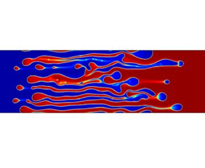
The evolution of the fully miscible VF (corresponding to System 1) is shown in figure 3(a). The fully miscible system without the Korteweg force  $\delta =0$ depicts a typical miscible fingering, which is very similar to that reported in Homsy (Reference Homsy1987), McCloud & Maher (Reference McCloud and Maher1995), Tan & Homsy (Reference Tan and Homsy1988) and Pramanik & Mishra (Reference Pramanik and Mishra2015b). By contrast, in partially miscible systems, a droplet formation was observed in all systems, as shown in figures 3(b)–3(d). As the strength of the phase separation and Korteweg force increases, the droplets become clear. The droplet observed here, which some of the white arrows depict, is a blue droplet of
  $c=0$ surrounded by the red zone of
  $c=1$. In addition, the droplet decreases in size because of the mutual solubility. This trend is more remarkable for the lower strength of the phase separation. These phenomena imply that phase separation and diffusion processes were observed. The importance here is that the transition from viscous fingering to a droplet pattern induced by an increase in the strength of the phase separation and the Korteweg force is in good agreement with previous experiment results (Suzuki et al. Reference Suzuki, Nagatsu, Mishra and Ban2020), where the transition was induced by an increase in the concentration of
  $\mbox {Na}_2 \mbox {SO}_4$. We also note that because of the diffusion, the interface in the standard fingering in fully miscible systems smoothly joins the states of
  $c = 1$ and
  $c = 0$ (figure 3a), whereas the interface between the two steady states remains sharp at any time as the phase separation becomes stronger (figures 3b–d).

Figure 3. Temporal evolution of the dimensionless concentration field for Systems (a) 1, (b) 2, (c) 3, and (d) 4. The dimensionless concentration field is shown at successive dimensionless times  $t= 1000$, 2000, 3000, 4000, from top to bottom. The scale bar is shown at the right. The droplet formation is indicated by the white arrows. Thin yellow arrows indicate the dissolution of the advancing finger, whereas a thick yellow arrow indicates the adjacent finger, which becomes the advancing finger after the dissolution.
In the previous numerical study that investigated the effect of  $Pe$ on fully miscible VF, Pramanik & Mishra (Reference Pramanik and Mishra2015b), the Péclet number was defined as
  $UL/D$, where
  $U$ is the velocity of the main flow,
  $L$ is the size of the computational domain, and
  $D$ is diffusivity, where VF was observed when
  $Pe$ has order of magnitude 1000. However, in the present study, even in the fully miscible system without phase separation, VF is observed under the condition
  $Pe = 5$, which is obviously smaller than that used in the previous typical numerical study (Pramanik & Mishra Reference Pramanik and Mishra2015b). This is due to the difference in the size of
  $L$. In the previous study (Pramanik & Mishra Reference Pramanik and Mishra2015b) and the present model, the dimensionless time is defined as
  $t^*=t/(L/U)$. If
  $L$ in Pramanik & Mishra (Reference Pramanik and Mishra2015b) is 200 times larger than
  $L$ in the present model, for the same
  $D$,
$D$,  $U$ and
  $t$, then in Pramanik & Mishra (Reference Pramanik and Mishra2015b)
  $Pe$ is 200 times larger than
  $Pe$ in the present model. On the other hand,
  $t^*$ in Pramanik & Mishra (Reference Pramanik and Mishra2015b) is 200 times smaller than
  $t^*$ in the present model. These indicate that for equivalent
  $Pe \times t^*$, we observe equivalent VF dynamics. In other words, the VF dynamics for
  $Pe = 5$ and
  $t^*=1000$ in the present model is equivalent for
  $Pe = 1000$ and
  $t^*= 5$ in figure 8(a) of Pramanik & Mishra (Reference Pramanik and Mishra2015b).
The mechanism of droplet formation was described in a previous study (Suzuki et al. Reference Suzuki, Nagatsu, Mishra and Ban2020) as follows. The experiments in Suzuki et al. (Reference Suzuki, Nagatsu, Mishra and Ban2020) employed an aqueous two-phase system that goes through thermodynamically unstable regions and a phase separation of a spinodal type. Such phase separation promotes a mass transfer against the concentration gradients, leading to a separation of the system into low- and high-concentration regions. Furthermore, the Korteweg force creates a spontaneous fluid convection, promoting a phase separation. These effects result in a pinching of the viscous fingers and eventually lead to the formation of droplets. The transition from fingering to droplet pattern formation by tuning  $\alpha _2$,
  $\alpha _3$ and
  $\delta$ shows theoretically that the nature of a phase separation and a spontaneous convection is the origin of the droplet formation. Thus the results shown in figure 3 verify this claim from the experimental study (Suzuki et al. Reference Suzuki, Nagatsu, Mishra and Ban2020). Another numerical study, by De Wit & Homsy (Reference De Wit and Homsy1999), reported the droplet formation in viscous fingering. In this numerical study, a fully miscible VF with a chemical reaction was simulated, which is similar to a phase separation, producing two fluids of low and high concentrations. When the composition falls in a region that corresponds to the spinodal region in the phase separation system, the system evolves spontaneously towards a chemically thermodynamic equilibrium. These effects result in a pinching of the viscous fingers and finally lead to the formation of droplets. Thus the numerical study by De Wit & Homsy (Reference De Wit and Homsy1999) showed that phase separation produces droplets in viscous fingering dynamics. Our numerical study includes a phase separation based on thermodynamic free energy and the Korteweg force, which was not considered by De Wit & Homsy (Reference De Wit and Homsy1999). Therefore, our mathematical model can simulate viscous fingering more realistically with a phase separation because the hydrodynamics and chemical thermodynamics are properly combined.
3.1. Phase separation effects on mixing length
We conducted several quantitative analyses. First, the mixing length was computed. To compute the mixing length, we first compute the two-dimensional concentration field of the concentration,  $c (x, y, t)$, which can be averaged along the transverse coordinate to yield one-dimensional transversely averaged concentration profiles
 \begin{equation} \displaystyle \langle c(x,t)\rangle =\frac{1}{L_y} \int_0^{L_y} c(x,y,t)\, {{\rm d} y}. \end{equation}
Here,  $\langle c(x,t)\rangle$ increases monotonically with
  $x$. The length of
  $x$, where
  $c$ is within the range
  $0.01 \leqslant c \leqslant 0.99$, is defined as the mixing length,
  $L$. The time evolution of
  $L$ is shown in figure 4(a). In System 1,
  $L$ grows as
  $L \propto t^{0.50}$ when
  $t$ is less than approximately 2500, whereas when
  $t$ is more than approximately 2500,
  $L$ grows almost linearly over time. Along with the observation of the displacement pattern, we found that the displacement grows diffusively without the formation of fingering during the early stage, and grows nearly linearly with
  $t$ with the formation of fingering during the later stage. This behaviour is very similar to that of a fully miscible VF with ordinary diffusion (Tan & Homsy Reference Tan and Homsy1988), where diffusion obey Fick's law. In Systems 2–4, the growth behaviour can also be divided into two types. The transient corresponds to the onset of the fingering. The growth during the early stage (
 $t \leqslant 600 \text {--}800$) was slower than that of System 1. As the strength of the phase separation increases, the early growth becomes slower. This could be because the phase separation suppresses the ordinary diffusion. The onset of fingering occurs later, as the strength of the phase separation becomes more intensive. The result can be explained as follows. In this model, the coefficient of the diffusion term is
  $\alpha _2 / Pe$ in (2.10). That is, the apparent
  $Pe$ is
  $Pe / \alpha _2$. In partially miscible systems, the value of
  $Pe / \alpha _2$ in the different systems follows System 2 > System 3 > System 4 (see table 1). The order of onset time also follows in a similar manner as System 2 < System 3 < System 4. It is considered that the reason why onset is the fastest (slowest) in System 2 (4) is that the apparent
  $Pe$ is the largest (smallest). It is accepted that the onset is earlier as
  $Pe$ is larger for fully miscible VF (Pramanik & Mishra Reference Pramanik and Mishra2015b). Furthermore, in the fully miscible case, because there is no Korteweg force (that is,
  $\delta = 0$) that acts to enhance the fingering, the onset can be considered to be the slowest. During the later stage, we fit the linear relation
  $L = v' t + a$, where
  $a$ is the intercept. The linear fitting was done in
  $2500 \leqslant t \leqslant 4000$ for System 1,
  $650 \leqslant t \leqslant 2050$ for System 2,
  $850 \leqslant t \leqslant 4000$ for System 3, and
  $900 \leqslant t \leqslant 4000$ for System 4. As shown in figure 4(a), the line for System 2 bends around
  $t = 2000$ and the fitting was done before
  $t = 2050$. More discussion about the bend is given later. We plot
  $v'$, which is the the average velocity during the above-mentioned period, as a function of
  $\alpha _2 \delta$ in the inset of figure 4(a), where four plots correspond to Systems 1–4 in descending order of the value of
  $\alpha _2 \delta$, and find that
  $v'$ increases with
  $\alpha _2 \delta$. In Systems 2–4, we changed simultaneously
  $\alpha _2$ and
  $\delta$ to make a comparison with the corresponding experiment (Suzuki et al. Reference Suzuki, Nagatsu, Mishra and Ban2020). As mentioned earlier, when both the values
  $\alpha _2$ and
  $\delta$ increase, the phase separation effects become larger. Thus the product of
  $\alpha _2 \delta$ can be considered an indicator of the strength of the phase separation effects.

Figure 4. (a) Results of the mixing length,  $L$, with time evolution. In the inset,
  $v'$ versus
  $\alpha _2 \delta$ is plotted. (b) Time evolution of
  $V'$ is shown for Systems 1–4. Note that the variables
  $L$,
$L$,  $t$,
$t$,  $v'$ and
  $V'$ are dimensionless.
In figure 4(b), we calculate the time derivative of  $L$, which is denoted as
  $V'$, which means the instantaneous finger velocity. In System 1, the velocity
  $V'$ initially decreases with
  $t$ and reaches a constant value before the onset of the fingering. After the onset (
 $t = 2500$),
  $V'$ increases due to the fingering formation. In Systems 2–4, we found that
  $V'$ increases with
  $t$ when
  $500 \leqslant t \leqslant 1000$. This is a unique characteristic of a phase separation system. Therefore, the behaviour of the velocity is a property that can distinguish qualitatively a system with a phase separation from a fully miscible system. The phase separation systems have finite values of
  $\delta$, which means that a Korteweg force acts. The existence of a Korteweg force is responsible for an increase in
  $V'$ with time when
  $500 < t < 1000$. In Systems 3 and 4,
  $V'$ reaches a constant value after the increase. In System 2, we noted that after the increase in the velocity during
  $500 \leqslant t \leqslant 1000$,
  $V'$ decreases (which corresponds to the bend of line in figure 4a) and then increases again. Along with the observation in figure 3, the temporal decrease could be due to a dissolution of the advancing finger (indicated by thin yellow arrows), and the temporal increase again could be due to a fingering growth of the adjacent finger (indicated by thick yellow arrows) after the dissolution. It should be noted that a temporal decrease of the mixing length due to the sudden fade away of droplets at the leading front of the mixing zone was also reported previously by De Wit & Homsy (Reference De Wit and Homsy1999), who investigated viscous fingering with a chemical reaction whose effect is equivalent to phase separation. Therefore, we consider that such non-monotonic behaviour of the velocity is inherent to a weak phase separation system. Based on the above, we claim that the velocity is a property that can distinguish three systems qualitatively: systems with strong phase separations, a weak phase separation, and no phase separation.
3.2. Phase separation effects on interfacial length
We next analyse the interfacial length  $I$, which is defined as (Mishra, Martin & De Wit Reference Mishra, Martin and De Wit2008; Pramanik & Mishra Reference Pramanik and Mishra2015a)
 \begin{equation} I(t)= \int_0^{L_y} \int_0^{L_x} \sqrt{ \left( \frac{ \partial c}{\partial x} \right)^2 + \left( \frac{ \partial c}{\partial y}\right )^2 } \,{\rm d}\kern0.7pt x\,{\rm d}y. \end{equation}
The temporal evolution of  $I$ is shown in figure 5. The vertical width of the computational domain is 256. In all systems, initially
  $I = 256$, which means that the interface is vertically flat, thus no fingering takes place. When the fingering is formed, the vertical interface is deviated and
  $I$ increases from 256. Therefore, a deviation from
  $I = 256$ indicates the onset of fingering. Thus figure 5(a) shows clearly that the onset occurs earlier in order of Systems 2, 3, 4 and 1. We also found that the onset occurs later when the phase separation is strong, from figure 4(a). After the onset, as the strength of the phase separation and Korteweg force increases,
  $I$ becomes larger, which means that the number of droplets increases. We show
  $I$ versus
  $L$ in the inset of figure 5(a). The results show that
  $I$ as a function of
  $L$ is always larger when the effects of the phase separation are stronger. This observation can be compared directly to the corresponding experimental results (Suzuki et al. Reference Suzuki, Nagatsu, Mishra and Ban2020). To do so, we measured the interfacial length of the displacement pattern
  $I_{exp}$, which is shown in figure 3 in Suzuki et al. (Reference Suzuki, Nagatsu, Mishra and Ban2020), as a function of the maximum radius of the pattern,
  $r_{max}$. The results show that
  $I_{exp}$ is mostly similar without regard to the concentration of
  $\mbox {Na}_2 \mbox {SO}_4$ for
  $r_{max} < 30$ mm, while
  $I_{exp}$ is larger as the concentration of
  $\mbox {Na}_2 \mbox {SO}_4$ is larger (the phase separation becomes stronger) for
  $r_{max} > 30$ mm. Figure 3 of Suzuki et al. (Reference Suzuki, Nagatsu, Mishra and Ban2020) shows that little droplets or only a small number of droplets are formed for
  $r_{max} < 30$ mm, while the number of droplets clearly increases with the concentration of
  $\mbox {Na}_2 \mbox {SO}_4$ at
  $r_{max} = 42$ mm. A comparison between the behaviour of
  $I_{exp}$ as a function of
  $r_{max}$ and visual observation of the fingering pattern as a function of
  $r_{max}$ demonstrates that the formation of the droplets increases the interfacial length. Based on this consideration and visual observation of the numerical results (figure 3), an increase of growth rate of
  $I$ with an increase in the phase separation effects should be attributed to the droplet formation. The inset of figure 5(a) in the numerical simulation and figure 5(b) in the corresponding experiment both show that the interfacial length as a function of the pattern size is almost the same without regard to the strength of the phase separation at an earlier stage before droplet formation, whereas it becomes larger with an increase in the strength of the phase separation at later stages after droplet formation. There, we find that the results shown in the inset of figure 5(a) in the numerical simulation and figure 5(b) in the corresponding experiment (Suzuki et al. Reference Suzuki, Nagatsu, Mishra and Ban2020) match extremely well.

Figure 5. Results on the interfacial length,  $I$: (a) time evolution of
  $I$, with inset
  $I$ as a function of
  $L$; and (b)
  $I_{exp}$ as a function of
  $r_{max}$ from Suzuki et al. (Reference Suzuki, Nagatsu, Mishra and Ban2020).
Regarding the geometry, the representative velocity is constant in the simulation of the rectilinear geometry, while it decreases with time in the experiment of the radial geometry. In the experiment of the radial geometry, the relative effect of Korteweg convection to convection by fluid injection is larger with time. The difference may affect the dynamics of the interfacial length,  $I$, quantitatively. In figure 5, the slope of the
  $I$ versus
  $L$ curve obtained from the simulation is gradually decreasing, while the slope of the
  $I_{exp}$ versus
  $r_{max}$ curve obtained from the experiment is gradually increasing, mostly. These results may be consistent with the relative effect of Korteweg convection to convection by fluid injection being larger in the experiment.
4. Conclusions
In conclusion, we established a numerical simulation of viscous fingering with a phase separation of the spinodal decomposition type, taking into account the Korteweg force. The simulation reproduced successfully the experimental observation in Suzuki et al. (Reference Suzuki, Nagatsu, Mishra and Ban2020) of the transition from viscous fingering to a droplet pattern owing to the increase in the phase separation effects. We show that the time derivative of the mixing length is a property that can qualitatively distinguish three systems: systems with strong phase separations, a weak phase separation, and no phase separation. Furthermore, the interfacial length as a function of the mixing length obtained in the simulation is in good agreement with the experiments of the previous study (Suzuki et al. Reference Suzuki, Nagatsu, Mishra and Ban2020).
In this paper, for the first time, we show mathematically that the fingering pattern transitions to the droplet pattern when the system transitions from fully miscible to partially miscible in the rectilinear geometry, which was observed in the experiment in the radial geometry, and that its origin is the effect of phase separation and Korteweg convection, by using a simple model that can effectively adjust the effects of phase separation. This indicates that the droplets observed in the experiment are not originated by the circular geometry. The difference in geometry between the experiment and simulation is not important to the objective and significance of this paper. This study provides successfully a mathematical model and numerical simulation that can reproduce the existing experimental results of viscous fingering with a phase separation. Therefore, this model and its simulation will be useful in elucidating the mechanism of the experimental results currently under investigation, such as the effect of the flow rate on the dynamics. In turn, new dynamics of VF with a phase separation will be obtainable through numerical experiments conducted using the proposed model, the results of which we will verify experimentally. Such collaboration between experimentation and numerical simulation will enable a comprehensive understanding of VF with a phase separation in partially miscible systems, which can contribute to establishing highly efficient processes involving VF with a phase separation in various fields such as enhanced oil recovery and  $\mbox {CO}_2$ sequestration.
Funding
This work was supported by JSPS KAKENHI Grant nos 19J12553 and 19K04189. M.M. gratefully acknowledge the JSPS Invitation Fellowships for Research in Japan (no. L19548).
Declaration of interests
The authors report no conflict of interest.


 Open access