Recognition of the Bare Soil Using Deep Machine Learning Methods to Create Maps of Arable Soil Degradation Based on the Analysis of Multi-Temporal Remote Sensing Data

Abstract

The detection of degraded soil distribution areas is an urgent task. It is difficult and very time consuming to solve this problem using ground methods. The modeling of degradation processes based on digital elevation models makes it possible to construct maps of potential degradation, which may differ from the actual spatial distribution of degradation. The use of remote sensing data (RSD) for soil degradation detection is very widespread. Most often, vegetation indices (indicative botany) have been used for this purpose. In this paper, we propose a method for constructing soil maps based on a multi-temporal analysis of the bare soil surface (BSS). It is an alternative method to the use of vegetation indices. The detection of the bare soil surface was carried out using the spectral neighborhood of the soil line (SNSL) technology. For the automatic recognition of BSS on each RSD image, computer vision based on deep machine learning (neural networks) was used. A dataset of 244 BSS distribution masks on 244 Landsat 4, 5, 7, and 8 scenes over 37 years was developed. Half of the dataset was used as a training sample (Landsat path/row 173/028). The other half was used as a test sample (Landsat path/row 174/027). Binary masks were sufficient for recognition. For each RSD pixel, value “1” was set when determining the BSS. In the absence of BSS, value “0” was set. The accuracy of the machine prediction of the presence of BSS was 75%. The detection of degradation was based on the average long-term spectral characteristics of the RED and NIR bands. The coefficient C_mean, which is the distance of the point with the average long-term values of RED and NIR from the origin of the spectral plane RED/NIR, was calculated as an integral characteristic of the mean long-term values. Higher long-term average values of spectral brightness served as indicators of the spread of soil degradation. To test the method of constructing soil degradation maps based on deep machine learning, an acceptance sample of 133 Landsat scenes of path/row 173/026 was used. On the territory of the acceptance sample, ground verifications of the maps of the coefficient C_mean were carried out. Ground verification showed that the values of this coefficient make it possible to estimate the content of organic matter in the plow horizon (R² = 0.841) and the thickness of the humus horizon (R² = 0.8599). In total, 80 soil pits were analyzed on an area of 649 ha on eight agricultural fields. Type I error (false positive) of degradation detection was 17.5%, and type II error (false negative) was 2.5%. During the determination of the presence of degradation by ground methods, 90% of the ground data coincided with the detection of degradation from RSD. Thus, the quality of machine learning for BSS recognition is sufficient for the construction of soil degradation maps. The SNSL technology allows us to create maps of soil degradation based on the long-term average spectral characteristics of the BSS.

1. Introduction

The spatial heterogeneity of the soil cover is the leading factor in the intra-field heterogeneity of the productivity of arable land. It is difficult to reveal the spatial intra-field heterogeneity of the soil cover, because this requires work with high cartographic accuracy at a scale of 1:10,000 and larger. For such scales, the instruction on soil mapping of 1973 applies to the territory of Russia [1]. Often, instead of soil cover mapping, various methods of indicative botany were used in the form of analyses of vegetation indices [2,3,4,5,6,7]. An alternative to vegetation indices is the method of constructing soil maps based on the analysis of the bare soil surface [8,9,10,11,12,13,14].

Maps of soil cover degradation can be based on modeling degradation processes [15,16,17,18]. Modeling requires the use of various data in addition to remote sensing data, such as climate data [19,20]. An important role in modeling degradation can be played by various characteristics of the relief: slopes, exposure, catchment area, etc. [21,22,23,24]. To calculate the relief characteristics, digital elevation models or digital terrain models are required [25,26]. Soil degradation maps obtained by modeling require groundwork, because even with the same relief characteristics (obtained from the DEM), degradation may or may not occur [8].

Big remote sensing data [27] open perspectives for constructing soil degradation maps. Partially big RSD can be processed by manual interpretation [28,29,30,31,32]. These methods include the method of retrospective monitoring of soil and land cover, which allows one to construct maps using RSD for a period of more than 50 years [33]. The accuracy of such works can exceed the accuracy of ground surveys [32,33,34]. The processing of big remote sensing data in the manual interpretation mode is very laborious. Despite the complexity, the method of retrospective monitoring of the soil and land cover is necessary to determine the boundaries of arable land, which are the boundary conditions for interpretation characteristics [35].

The possibility of identifying degradation foci based on RSD is confirmed by the breadth of coverage of such studies in different countries and on different continents [36,37,38]. These are modern methods for automating the mapping of land degradation [39,40,41]. RSD time series analysis approaches were used much less frequently in the construction of maps [38]. It can be assumed that the analysis of big satellite data [7,27,42] makes it possible to create maps of land degradation. The issue is the choice of the RSD processing method.

Working with big data is, first of all, Data mining and MapReduce [8]. When working with big RSD, it is necessary to select RSD suitable for calculations and analysis and reject unsuitable ones. Unsuitable images include images or fragments of images with clouds. Clouds masks are in open access [43]. The disadvantages of existing cloud masks require new filtering methods based on deep machine learning and computer vision [6,44,45,46,47]. It can be assumed that the use of deep machine learning will make it possible to select the necessary satellite images. In this mode, deep machine learning will allow data mining procedures [48,49] for big satellite data [27,42]. The issue is the choice of filtering methods.

Convolutional neural networks are widely used in solving various problems: for calculating the heat radiation of windows [50], for assessing land use changes over long periods of time (1990–2017) [51], and for mapping temperature anomalies in cities [52]. Convolutional neural networks (CNN) in processing color (RGB) images of the earth’s surface from various data sources can increase the accuracy of calculations and reduce labor costs in plant recognition: detection and counting of palm trees [53], recognition of coffee crops [54], detection of Ziziphus lotus [55], classification of crops and vegetation [56].

Machine learning is also used in thematic interpretation [57,58]. Mapping of erosion distribution is one of the types of thematic interpretation [59,60]. In an integrated approach, machine learning is applied to a set of factors [59,60], but can also be applied to RSD only [61,62]. During thematic interpretation, areas with same spectral brightness or values of calculated indices were distinguished [36,40,41]. Often, when degradation is recognized, sites with reduced yields are searched for [57,62,63]. When analyzing long-term observation series, areas are selected where a reduced yield is recorded most often [6,63,64]. It can be assumed that areas of agricultural fields with uniform spectral characteristics recorded over many years can be an indicator of the state of the soil cover.

Intra-field heterogeneity maps based on long-term RSD data are widely used by commercial structures: ExactFarming [65], Farmers Edge [66], Cropio [67], Intterra [68], AGRO-SAT [69], NEXT farming [63], Agronote [70]. It can be assumed that the processing of multi-temporal data is highly efficient for detecting intra-field heterogeneity.

In the work of 2020 [7], the result of applying the method of averaging long-term vegetation indices is presented. A 2021 article [6] outlines the application of the frequency filter method for multi-year vegetation indices. Both methods are, in one way or another, methods of indicator botany. The work of 2021 [9] outlines the method of averaging vegetation indices adjusted for the methods of analysis of the spectral neighborhood of the soil line (SNSL). The SNSL theory itself is presented in a series of works of 2016–2018 [10,11,12,13,14]. The SNSL theory assumes the possibility of revealing the spatial heterogeneity of the soil cover on the basis of big satellite data, but without the use of indicator botany.

We made several hypotheses:

• Soil cover degradation can be detected based on the recognition of bare soil surface in the analysis of big satellite data.
• The selection of satellite imagery to define the bare soil surface can be performed using deep machine learning methods.
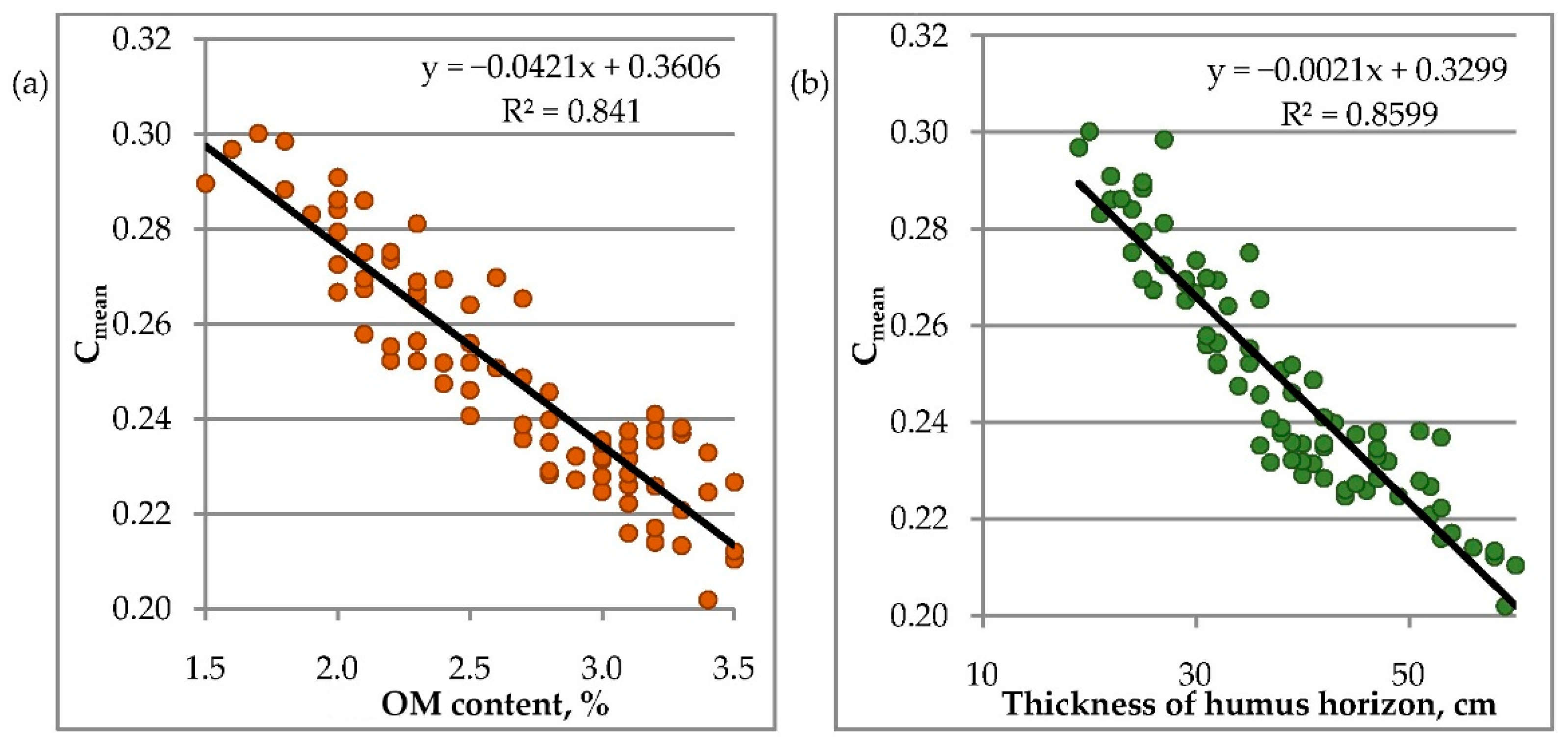
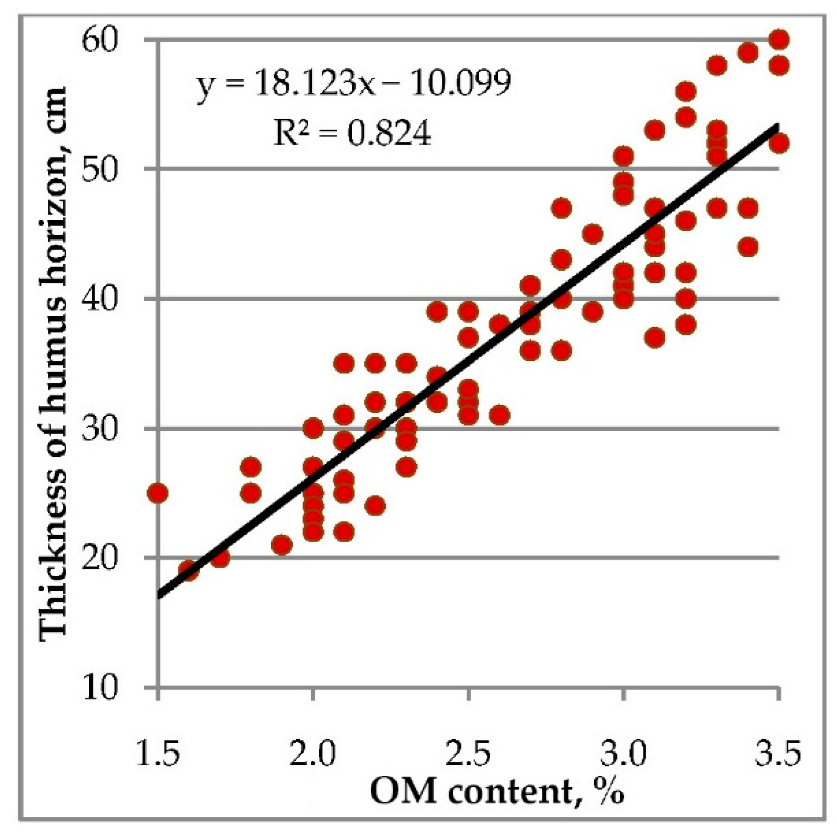
• An indicator of distribution of degradation can be the average long-term deviations of spectral brightness from the average spectral brightness characteristics of an agricultural field.
• It is possible to verify the results of identifying degradation areas by ground methods.
• Boundary conditions for identifying soil degradation areas can be defined by the method of retrospective monitoring of land use and soil cover.

The aim of the work is to develop a method for detecting degraded areas of arable land in the south of the European part of Russia based on the recognition of bare soil surface on satellite images using deep machine learning methods and methods for calculating average long-term values of the spectral brightness of the bare soil surface.

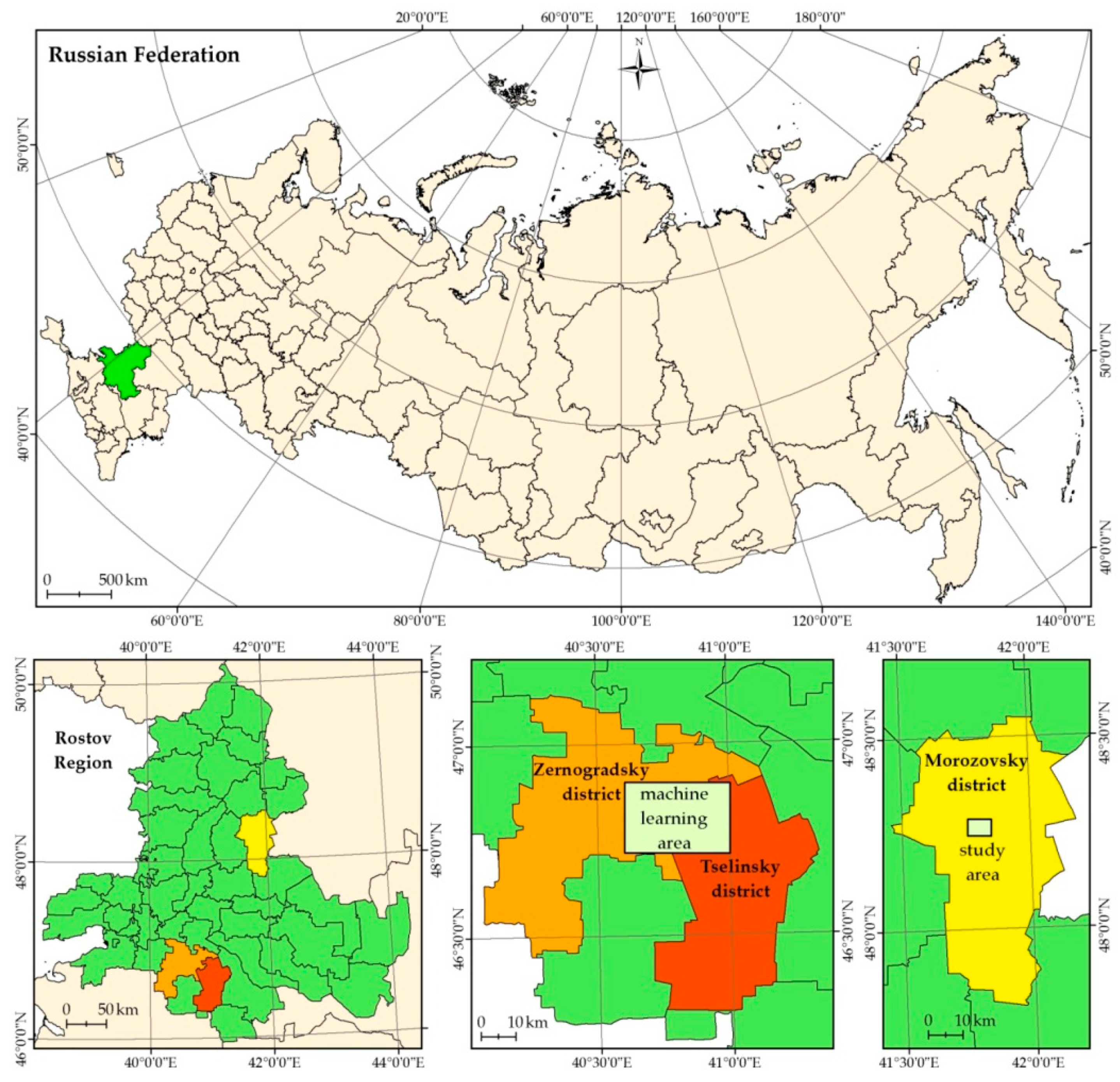
2. Materials and Methods

The study area is located on the territory of Russia in the Morozovsky district of the Rostov region (Figure 1). The soil cover is represented by dark chestnut slightly solonetzic clayey and heavy loamy soils on loess-like clays and loams (Haplic Kastanozems). The absolute height is about 120 m asl. The mean annual air temperature is 8.5 °C. The mean annual precipitation is 415.6 mm. Deep machine learning included Landsat scenes of path/row 173/028 and 174/027 for the area in the Zernogradsky and Tselinsky districts of Rostov region (Figure 1).

2.1. Creating a Map of Arable Lands Boundaries

The boundaries of arable lands were created by the method of retrospective monitoring of the soil and land cover [33]. In the course of retrospective monitoring, the boundaries of the agricultural fields were determined by interpretation of the RSD for 50 years. Particular attention is paid to the period from 1984 to 2020 (35 years). In this time interval in Russia, the sown area decreased from 117 million ha (1990) to 74 million ha (2007) [71]. In terms of accuracy, the method of retrospective monitoring surpasses traditional mapping at a scale of 1:10,000 [33,35] (Figure 2). Remote sensing data of different spatial resolution were analyzed: high spatial resolution (IKONOS, GeoEye-1, WorldView, etc.) [72], medium spatial resolution (Landsat, Sentinel) [43], and archival data of 1968 and 1975 (CORONA) [73]. The quality and accuracy of interpretation are checked using topographic maps at a scale of 1:25,000 (Figure 2c).

2.2. Dataset Development

The bare soil surface occupies an elliptical region in the spectral space of RED and NIR bands [13] (Figure 3)—the spectral neighborhood of the soil line (SNSL). This area is part of tasseled cap [74] and lies on the soil line [74] between areas of stubble residues (straw) and traces of agricultural fires (soot), which are abundant in southern Russia [75]. The location of SNSL only partially coincides with the soil line for vegetation indices such as the NDVI [76].

The dataset was made of RSD of 1984–2020. In total, 1028 Landsat scenes were found and downloaded from the archives. To form the dataset, 244 Landsat 4, 5, 7 and 8 scenes were selected for two paths/rows-173/028 and 174/027 (Tables S1 and S2). The location of analyzed Landsat scene fragments is given on Figure 1. The choice of Landsat data is due to the large temporal coverage (1984–2022), the same spatial resolution (30 m), an identical set of spectral bands (Blue, Green, Red, NIR, SWIR1, SWIR2), well-known spectral and atmospheric correction algorithms.

For each of 244 Landsat scenes (Figure 4a,b), a graph of the frequency of occurrence of pairs of RED and NIR values (tasseled caps) [13] (Figure 4c,d) was plotted. On each graph, the areas of RED and NIR values for the bare soil surface were manually selected (Figure 4c,d). The areas highlighted on the graphs were transferred to the satellite image in the form of masks of the open soil surface (Figure 4e,f). The selection of BSS was corrected using a satellite image in the RGB mode (Figure 4a,b).

Thus, bare soil masks were built for 244 out of 1028 Landsat scenes using SNSL technology (Figure 4). A set of bare soil surface masks is a dataset for training a neural network. Half of the dataset (122 masks, Landsat path/row 173/028) was used as a training sample (Table S1). The second half of the dataset (122 masks, Landsat path/row 174/027) was used as a test sample (Table S2). The area of the bare soil surface varied on Landsat scenes from 1.5 to 54.8%.

The dataset is binary. For each pixel of each Landsat image, the mask can have only one of the two values “1” or “0”, i.e., bare soil surface or not. Classification of other objects identified in the RED-NIR spectral space was not carried out.

The learning element in the dataset is a pixel. For 244 images, an array of 567,127,808 training elements was created. The bare soil surface was identified on 112,632,627 pixels. Six Landsat spectral bands were used in machine learning: Blue, Green, Red, NIR, SWIR1, SWIR2.

In addition to the graphics mode in the RED-NIR spectral space (Figure 4c,d), the RGB mode was used to form the dataset. Images displayed as RGB represent the stack of three bands 7 (SWIR), 4 (NIR), 2 (Green) of Landast 7 (Figure 4a,b). The selection of the bare soil surface was carried out by three operators independently; each of the operators analyzed all 244 images in graphics mode and RGB mode. The resulting masks were compared with each other. For Landsat pixels in which a discrepancy in BSS identification was found, a value was assigned by a simple majority. Examples of bare soil surface masks are shown in Figure 4e,f.

Landsat images of path/row 173/026 for the territory of eight agricultural fields were used as an acceptance sample in this study (Figure 1 and Figure 2). The acceptance sample consists of 133 Landsat 4, 5, 7 and 8 scenes from 1985 to 2021 (Table S3).

2.3. Methods for Assessing the Quality of Machine Learning Algorithms

• Test sample. A set of objects not used in learning.
• Acceptance sample. An independent set of objects not used in development.
• Cross-validation (CV) [77,78]. The training sample is divided into N parts and training is performed N times on N − 1 parts (without repetitions).

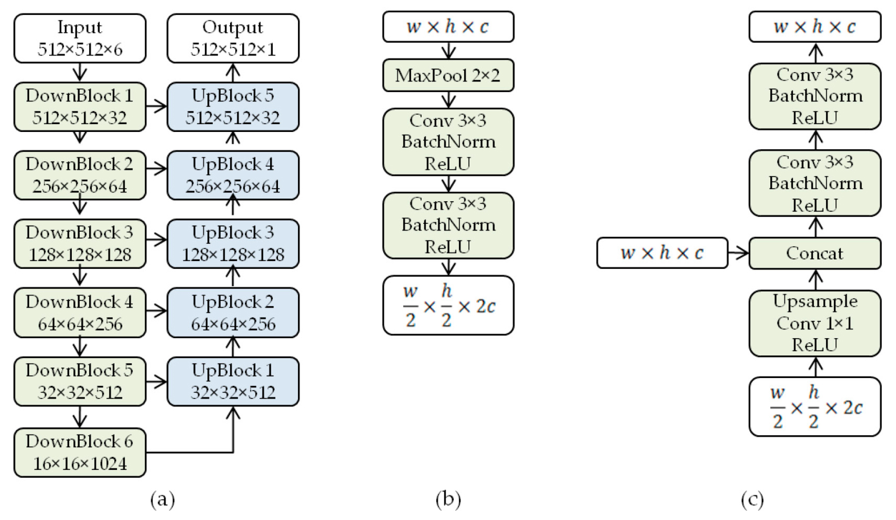
2.4. Deep Machine Learning, Convolutional Neural Networks Method

2.4.1. Model

We formulate the bare soil recognition on given satellite images as a per-pixel binary classification task. Thus, given an image $I$ of shape $W\times H\times C$, we expect the model to output $M$, an image of shape $W\times H$, where $M_{ij}\in \left[0,1\right]$ is the probability that $\left(i, j\right)$ pixel belongs to the bare soil region. $W$ and $H$ denote the width and height of the input image, and $C$ is the number of input bands. In computer vision, such a task is typically formulated as a binary image segmentation problem. Nowadays, deep neural networks [79] have become the standard approach to solving various computer vision tasks, including image segmentation. Deep neural networks were employed to address segmentation tasks in autonomous driving [80], medical image diagnosis [81,82], geo sensing [83,84], and precision agriculture [85,86].

The most popular neural architecture for image segmentation is U-Net [84], developed for biomedical image segmentation. U-Net consists of two parts: the encoder part processes input image and reduces its spatial dimensions, and the decoder part accepts encoder output and predicts the mask of the same size as the input image. Typically, the encoder and the decoder are built from the same number of convolutional blocks; this number is a matter of choice. The downsampling block (in the encoder) and the upsampling block (in the decoder) of the same size are connected via a skip connection. The neural architecture of our model is depicted in Figure 5.

Each encoder block contains a maximum pooling layer with a stride of 2 and two convolutional layers with a kernel size of 3, each followed by normalization and activation layers. Each decoder block accepts two inputs: an output of the corresponding encoder block of shape $w\times h\times c$ and the output of the previous decoder block of shape $\frac{w}{2}\times \frac{h}{2}\times 2c$. The second input is upsampled to $w\times h\times c$, then processed with a single convolutional layer with a kernel size of 1 and concatenated with the first input. The resulting tensor is passed through two convolutional layers with a kernel size of 3, each followed by normalization and activation layers.

We use the ReLU activation function and apply batch normalization [87] in all downsampling and upsampling blocks. Sigmoid function serves as an activation function of the last layer so the model returns probabilities $M_{ij}\in \left[0,1\right]$.

2.4.2. Training

Our dataset contains 244 images of shape approximately 1300 × 1800 pixels. We split the data into two equal parts: 122 images are used for training, and the remaining 122 images comprise the validation subset. More specifically, the training part contains Landsat scenes path/row 173/028, and scenes path/row 174/027 are used for validation. Each image in the dataset is represented in the 6-channel form: Red, Green, Blue, NIR, SWIR1, and SWIR2.

We use the Dice loss [88], which is the standard choice for imbalanced classes. Accordingly, a bare soil mask always has much fewer pixels than the background.

$$DL\left(M,Q\right)=1-\frac{2{{\displaystyle \sum }}_{ij}{M}_{ij}{Q}_{ij}+1}{{{\displaystyle \sum }}_{ij}{M}_{ij}+{{\displaystyle \sum }}_{ij}{Q}_{ij}+1}$$

Here, $Q$ are the ground truth labels, $Q_{ij}\in \left\{0,1\right\}$, and $Q_{ij}=1$ only if $\left(i, j\right)$ pixel belongs to the bare soil surface.

We train our model by minimizing the loss function with Adam optimizer [89]. We set an initial learning rate to 0.01, then decay the learning rate 10 times after the 32nd and the 42nd epochs. The training is performed for 48 epochs in total. Each batch consists of 8 random 512 × 512 pixels crops of the images from the training part. Additionally, we apply random horizontal and vertical flips. In all our experiments, we utilize a single Nvidia RTX 2080ti GPU.

2.4.3. Validation

During validation, we take 512 × 512 pixels crops from all images in the validation subset. We calculate the intersection over union (IoU) between the predicted and the corresponding manually constructed bare soil masks (Figure 6).

$$IoU\left(\widehat{M},Q\right)=1-\frac{{{\displaystyle \sum }}_{ij}{\widehat{M}}_{ij}{Q}_{ij}}{{{\displaystyle \sum }}_{ij}{\widehat{M}}_{ij}+{{\displaystyle \sum }}_{ij}{Q}_{ij}-{{\displaystyle \sum }}_{ij}{\widehat{M}}_{ij}{Q}_{ij}}$$

Here, $\widehat{M}$ is $M$ thresholded by 0.5: ${\widehat{M}}_{ij}=M_{ij}>0.5$. The overall IoU score of the proposed model on the validation set is 0.79.

2.4.4. Evaluation

The model used in further experiments is trained on both train and validation splits. To process the high-resolution satellite images, we divide them into overlapping patches of 512 × 512 pixels with the step of 256 pixels by both axes. We estimate the mask with our model for all patches and aggregate patch masks to obtain a full-sized mask. We noticed that simple averaging causes visual artifacts: a grid with 256-pixel periodicity appears. To mitigate such unwanted edge effects, we combine the predictions from different patches with Gaussian weights.

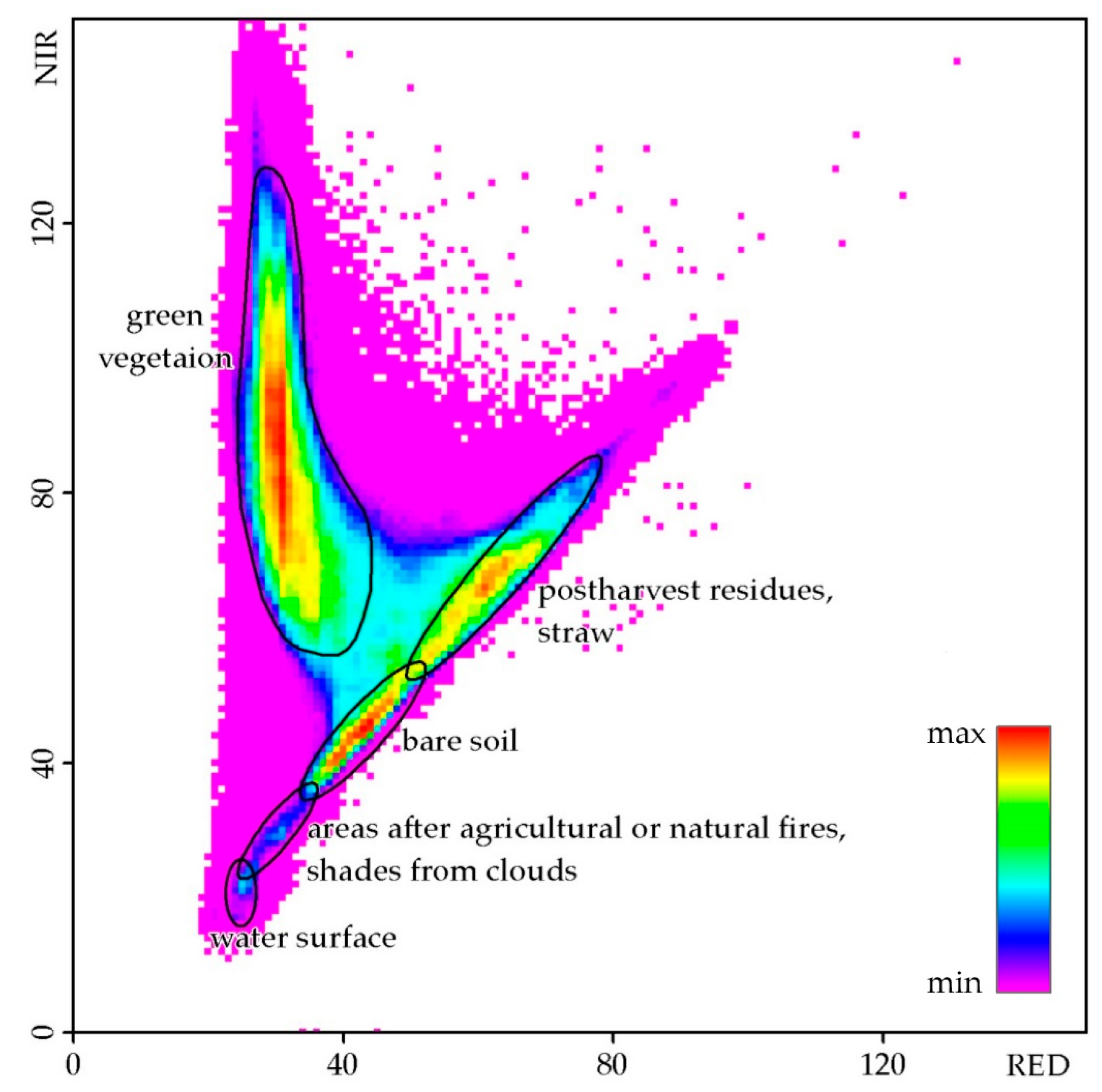
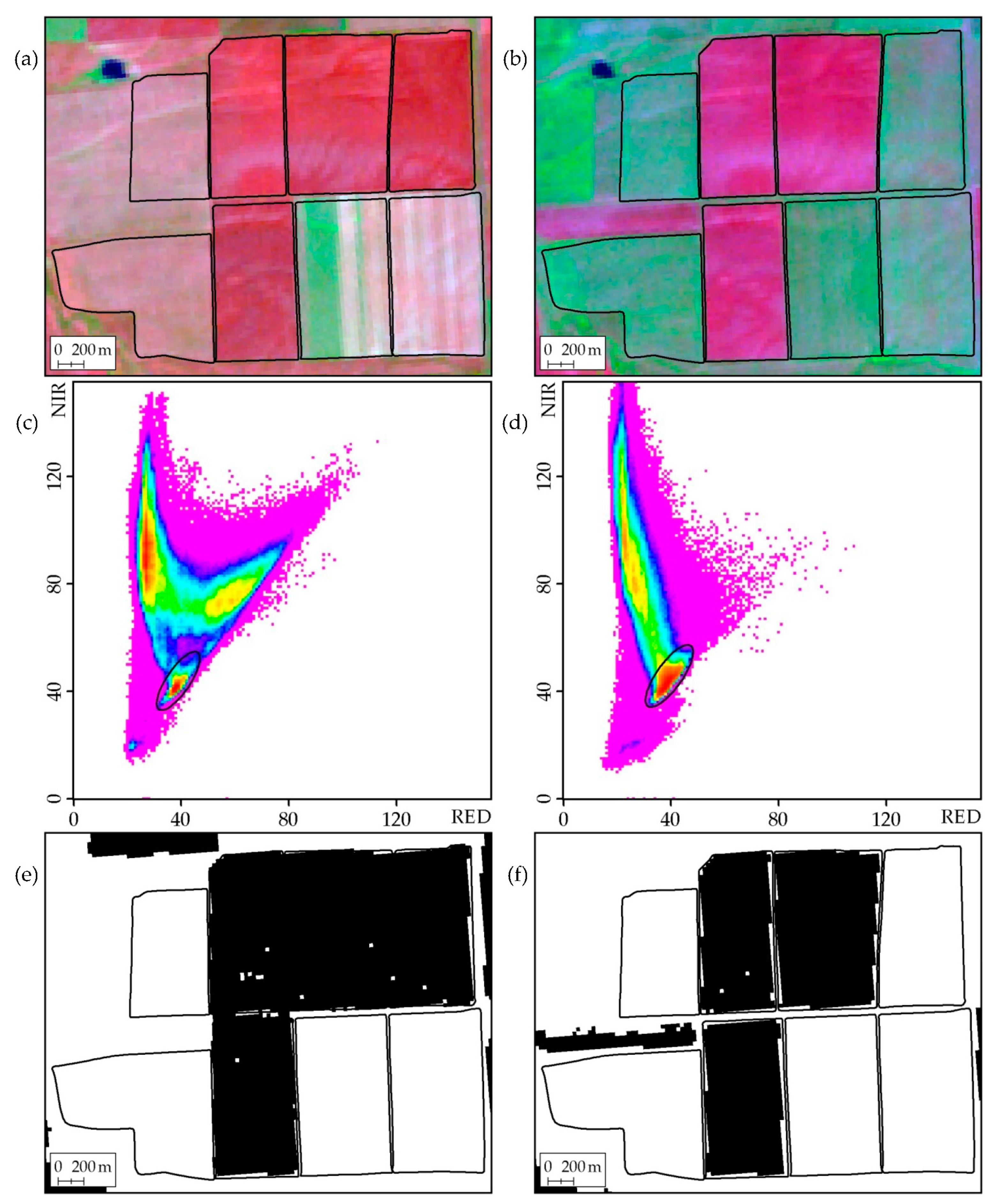
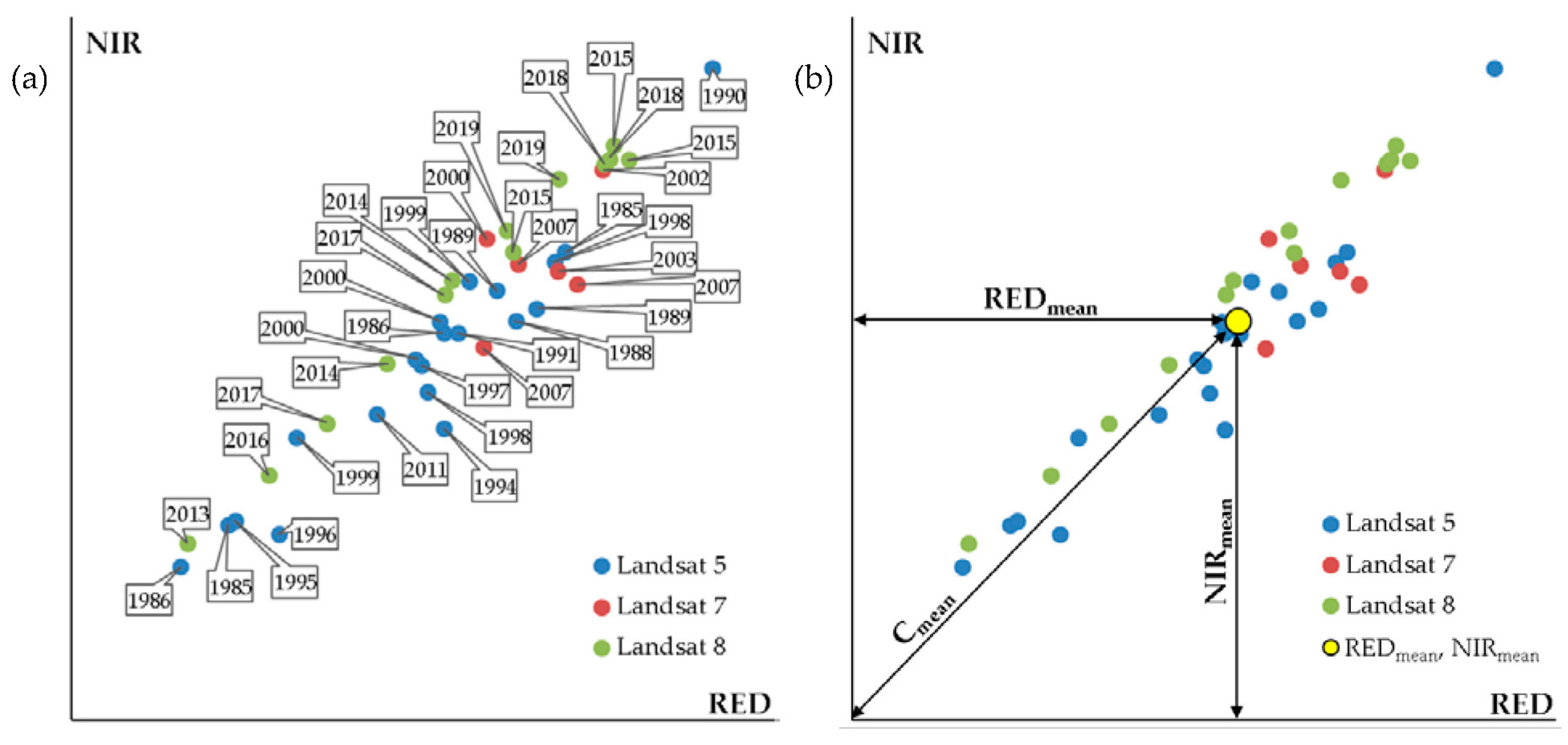
2.5. Calculation of the Average Multi-Temporal Values of the RED and NIR Spectral Bands for the Bare Soil Surface

The average multi-temporal values of the RED and NIR bands for the BSS were calculated for each Landsat pixel. According to the SNSL technology, the averaged multi-temporal RED and NIR spectral characteristics of the open soil surface are informative for constructing soil maps.

Figure 7a show a diagram of the position of the BSS RED and NIR values for one Landsat data pixel for the period from 1984 to 2020.

The RED values for a pixel are averaged using the formula:

$$RE{D}_{mean}=\left({\displaystyle \sum }_{i=1}^{n}RE{D}_i\right)/n$$

Here $RE{D}_i$—BSS RED value for $i$-th Landsat scene, $i$—Landsat scene number in the Landsat scenes database, $n$—total number of Landsat scenes in the Landsat scenes database involved in the calculation of long-term averages, $RE{D}_{mean}$—average long-term RED value for a pixel.

The NIR values for a pixel are averaged using the formula:

$$NI{R}_{mean}=\left({\displaystyle \sum }_{i=1}^{n}NI{R}_i\right)/n$$

Here $NI{R}_i$—BSS NIR value for $i$-th Landsat scene, $i$—Landsat scene number in the Landsat scenes database, $n$—total number of Landsat scenes in the Landsat scenes database involved in the calculation of long-term averages, $NI{R}_{mean}$—average long-term NIR value for a pixel.

2.6. Calculation of the Average Multi-Temporal Distance of a Set of RED and NIR Values for the BSS (C_mean Coefficient Calculation)

The average multi-temporal distance of a set of RED and NIR values for the BSS was calculated for each Landsat pixel. According to the SNSL technology, the long-term average distance of a point with long-term average RED and NIR values from the origin of coordinates has the best information content.

Figure 7b shows the location of the point of long-term average values of RED and NIR for the bare soil surface and its distance from the origin of coordinates. The distance between a point with long-term average RED and NIR values for each pixel is calculated by the formula:

$$C_{mean}=\sqrt{RE{D}_{mean}^2+NI{R}_{mean}^2}$$

Here $C_{mean}$ is the distance to a point with average long-term values of RED and NIR from the origin, $RE{D}_{mean}$—average long-term RED value for a pixel, $NI{R}_{mean}$—average long-term NIR value for a pixel.

2.7. Maps of C_mean Coefficient Values

The C_mean coefficient map is a map of distances from the origin to points with long-term average RED and NIR values for the open soil surface. The C_mean values were calculated with a spatial resolution of 30 m for the entire study area. This results in a matrix of C_mean values. In raster form, the matrix of C_mean values is shown on Figure 8.

2.8. Identification of Degradation Areas on the Map of C_mean Coefficient Values

The area of distribution of soil cover degradation on the map of C_mean values was understood as the area of C_mean values above the threshold determined in the course of the studies. We study the very possibility of soil mapping based on the analysis of multi-temporal spectral brightness of the bare soil surface. The threshold values were selected empirically based on ground surveys.

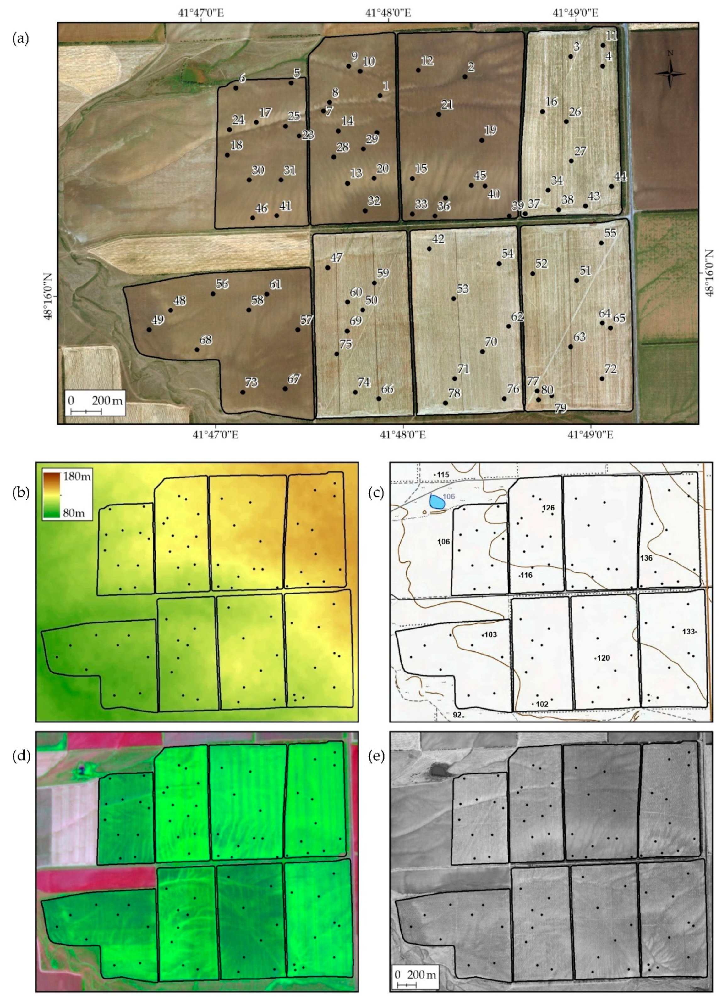
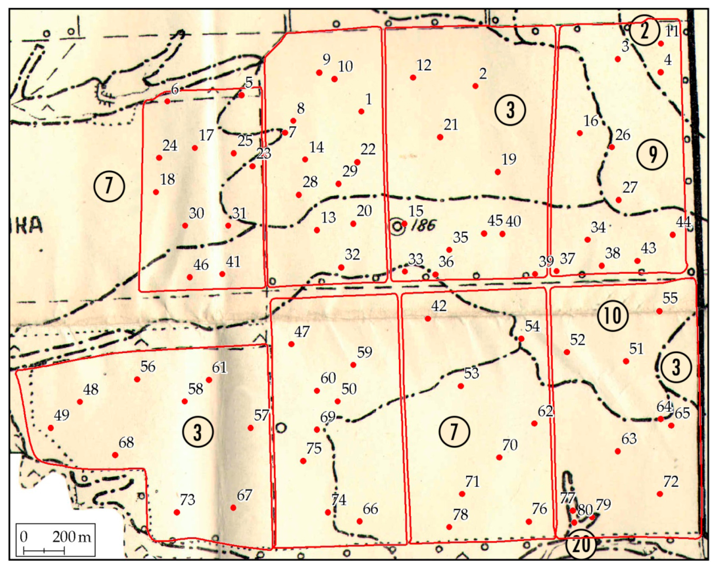
2.9. Ground Verification

To check the information content and establish the ranges of C_mean values for various soil varieties, ground verification was carried out. The soil pits were positioned and analyzed by classical methods based on methodological recommendations for field soil examination [1]. The ground survey is planned and carried out independently of the mapping of soil cover and soil degradation based on the analysis of the open soil surface. The maps obtained during the calculations were not provided to the field survey group. Topographic maps and orthophotomaps were used to determine the locations of ground sampling. On their basis, research routes were outlined. At each point with the planned coordinates, a soil pit was made. For each soil pit, a soil description, photographing, and sampling were carried out. The coordinates of the soil pits were recorded by a GPS receiver.

Route ground surveys were carried out in 2021. A total of 80 soil pits were made on eight agricultural arable fields. Soil samples were taken for agrochemical analysis. The total survey area was 649 ha. The thickness of the humus horizon and the content of organic matter (OM) were measured (

Table 1. Determination of soil degradation according to various criteria.

Soil Pit	OM Content, %	Thickness of Humus Horizon, cm	Soil Number *	Presence of Degradation According to Ground Survey Based on:			Cmean	Soil Pit Belongs to the Degradation Area Based on Cmean Value
				OM Content	OM Horizon	One of Two Signs
1	2.6	31	4	+	+	+	0.269858	+
2	3.5	60	1	-	-	-	0.210424	-
3	2.7	39	3	-	+	+	0.235787	-
4	3.1	53	2	-	-	-	0.215998	-
5	2.8	47	2	-	-	-	0.228312	-
6	3.0	42	2	-	-	-	0.234865	-
7	2.8	36	3	-	+	+	0.235183	-
8	2.7	36	3	-	+	+	0.265439	+
9	2.3	29	4	+	+	+	0.268917	+
10	3.3	47	2	-	-	-	0.238082	-
11	3.2	54	1	-	-	-	0.217113	-
12	2.8	40	2	-	-	-	0.229126	-
13	1.8	27	4	+	+	+	0.298548	+
14	3.2	38	3	-	+	+	0.237733	-
15	1.8	25	5	+	+	+	0.288368	+
16	3.2	56	1	-	-	-	0.214088	-
17	1.5	25	5	+	+	+	0.289702	+
18	3.1	37	3	-	+	+	0.231722	-
19	2.9	39	3	-	+	+	0.232223	-
20	1.7	20	5	+	+	+	0.300192	+
21	3.4	44	2	-	-	-	0.224676	-
22	3.2	42	2	-	-	-	0.241021	-
23	3.0	51	2	-	-	-	0.227908	-
24	1.9	21	5	+	+	+	0.283136	+
25	2.5	37	3	+	+	+	0.240682	-
26	3.1	53	2	-	-	-	0.222253	-
27	2.1	31	4	+	+	+	0.257937	+
28	2.2	35	3	+	+	+	0.255329	+
29	2.8	36	3	-	+	+	0.245738	+
30	2.2	32	3	+	+	+	0.252331	+
31	2.7	41	2	-	-	-	0.248755	+
32	3.2	40	2	-	-	-	0.235532	-
33	2.8	43	2	-	-	-	0.239885	-
34	2.0	23	5	+	+	+	0.286224	+
35	2.5	33	3	+	+	+	0.264084	+
36	3.0	41	2	-	-	-	0.231409	-
37	3.5	52	2	-	-	-	0.226734	-
38	3.0	48	2	-	-	-	0.231922	-
39	3.0	40	2	-	-	-	0.231901	-
40	2.0	25	5	+	+	+	0.279424	+
41	2.3	29	4	+	+	+	0.265249	+
42	2.7	38	3	-	+	+	0.238856	-
43	2.0	22	5	+	+	+	0.290922	+
44	2.3	27	4	+	+	+	0.281172	+
45	2.0	27	4	+	+	+	0.272576	+
46	2.1	25	5	+	+	+	0.269552	+
47	3.1	47	2	-	-	-	0.234590	-
48	2.1	35	3	+	+	+	0.275097	+
49	3.3	53	2	-	-	-	0.236870	-
50	2.1	29	4	+	+	+	0.269566	+
51	2.3	30	4	+	+	+	0.266714	+
52	3.2	46	2	-	-	-	0.225910	-
53	3.0	49	2	-	-	-	0.224724	-
54	3.5	58	1	-	-	-	0.212186	-
55	3.0	42	2	-	-	-	0.235597	-
56	2.5	32	3	+	+	+	0.251919	+
57	2.5	39	3	+	+	+	0.246120	+
58	2.1	26	4	+	+	+	0.267368	+
59	2.6	38	3	+	+	+	0.250798	+
60	2.3	35	3	+	+	+	0.252240	+
61	2.4	39	3	+	+	+	0.251858	+
62	3.4	59	1	-	-	-	0.201962	-
63	3.3	58	1	-	-	-	0.213384	-
64	2.2	30	4	+	+	+	0.273555	+
65	3.1	42	2	-	-	-	0.228488	-
66	2.0	30	4	+	+	+	0.266775	+
67	3.1	44	2	-	-	-	0.226033	-
68	2.0	24	5	+	+	+	0.284077	+
69	3.3	51	2	-	-	-	0.238200	-
70	2.9	45	2	-	-	-	0.227276	-
71	2.5	31	4	+	+	+	0.255995	+
72	3.3	52	2	-	-	-	0.220846	-
73	2.3	32	3	+	+	+	0.256425	+
74	2.4	34	3	+	+	+	0.247516	+
75	3.1	45	2	-	-	-	0.237499	-
76	2.1	22	5	+	+	+	0.286072	+
77	1.6	19	5	+	+	+	0.296866	+
78	2.4	32	3	+	+	+	0.269443	+
79	2.2	24	5	+	+	+	0.275200	+
80	3.4	47	2	-	-	-	0.232959	-

* soil names are given in Table 2.

). The humus horizon is the A horizon. A horizons: Mineral horizons which formed at the surface or below an O horizon, in which all or much of the original rock structure has been obliterated and which are characterized by one or more of the following: an accumulation of humified organic matter intimately mixed with the mineral fraction and not displaying properties characteristic of E or B horizons (see below); properties resulting from cultivation, pasturing, or similar kinds of disturbance; or a morphology which is different from the underlying B or C horizon, resulting from processes related to the surface [90]. Organic matter content was determined according to Tyurin [91]. A direct analog of Tyurin’s method for determining OM is the Walkley-Black method [92]. The locations of sampling and measurements of the thickness of the humus horizon are shown in Figure 2 and Figure 8 and Table 1.

When describing soil profiles and using the values of the OM content in the plow horizon and the thickness of the humus horizon, the type and subtype of soil and the presence of degradation were determined. The presence of soil degradation was determined during a field soil survey according to the methodological recommendations for a field survey [1]. In the methodological recommendations, degradation is understood as a decrease in the thickness of the humus horizon and/or a decrease in the OM content in the plow horizon compared to typical for a given soil under given conditions. The threshold values of the OM content and the thickness of the humus horizon (2.7% and 40 cm), as characteristics of degradation, were also determined during the field survey based on the typical characteristics of soil types and subtypes in the study area.

The quality of the interpretation was estimated by the percentage of coincidence of degradation definitions from ground surveys and the calculation of C_mean values obtained by automated interpretation of multi-temporal RSD arrays. The results are presented in Table 1.

2.10. Cartographic Analysis

AcrGIS was used for cartographic analysis [93]. All materials were combined in this GIS. The main method of analysis was the pairwise intersection of different layers of the GIS project. The results of the intersection were recorded in tables. The quantitative parameters of the resulting combinations were evaluated and regression equations were determined.

2.11. GIS Project

For the territory of the Morozovsky district of the Rostov region, a GIS project was assembled, including the following layers:

• Topographic maps at scales of 1:25,000 and 1:50,000.
• Panchromatic aerial photography (2012) with a spatial resolution of 0.6 m (orthophotomap).
• Digital elevation model Shuttle radar topographic mission (SRTM) [26], horizontal resolution is 1 arc second and vertical resolution is 1 m.
• Scanned analogue space imagery of 1968 with a spatial resolution of 1.8 m (panchromatic, KH-4B satellite, US CORONA mission).
• Scanned analogue space imagery of 1975 with a spatial resolution of 6 m (panchromatic, KH-9 satellite, US CORONA mission).
• RSD Landsat 4, 5, 7 and 8 1985–2021 (133 scenes).
• RSD Sentinel-2 2016–2021 (224 tiles).

All materials used in the work have accurate georeferencing based on large-scale topographic maps. Local-affine transformations were used for exact georeferencing. For aerial photography and the US CORONA mission data, atmospheric correction was not performed. The ATCOR module of the ERDAS imagine software package [94] was used for Landsat and Sentinel data atmospheric correction.

The GIS project was used for determination of field boundaries using the technology of retrospective monitoring and organization of ground surveys. Only Landsat data were used in the calculation of C_mean maps and soil degradation maps using deep machine learning (Table S3).

3. Results

3.1. Deep Machine Learning: Implementation of the Method of Convolutional Neural Networks

During the implementation of machine learning, 133 masks of bare soil for the Landsat path/row 173/026 (Table S3) were constructed for 889,525 prediction elements for eight agricultural fields (Figure 2). The spectral brightness in the RED and NIR channels for the open soil surface was averaged over 35 years over all Landsat scenes for each pixel. The long-term average spectral brightnesses of RED and NIR were used as coordinates of the position of each Landsat pixel in the spectral space of RED and NIR. The distance to the point with average long-term values of RED and NIR from the origin of coordinates is taken as a characteristic of the soil cover and its degradation in the form of the C_mean coefficient. The map of C_mean coefficient values was constructed for eight agricultural fields (Figure 2).

No ground or other calibration data are required to map C_mean values. Only Landsat data were used in the calculations for the construction of soil maps and soil degradation maps using deep machine learning. The maps were built before ground verification surveys. In this regard, the proposed method is similar to the method of identifying degraded areas of arable land based on the frequency filter of NDVI binary masks [6] or the long-term average EVI+ [7,95].

The choice of eight fields for the formation of the acceptance sample is due to the possibility of ground surveys. The territory of groundworks is selected and limited by the owner of agricultural land.

3.2. Additions to the GIS Project

After predicting the presence of the bare soil surface on the RSD, the following layers were added to the GIS project:

8.

Scheme of agricultural fields (limits of distribution of calculations of the coefficient C_mean).

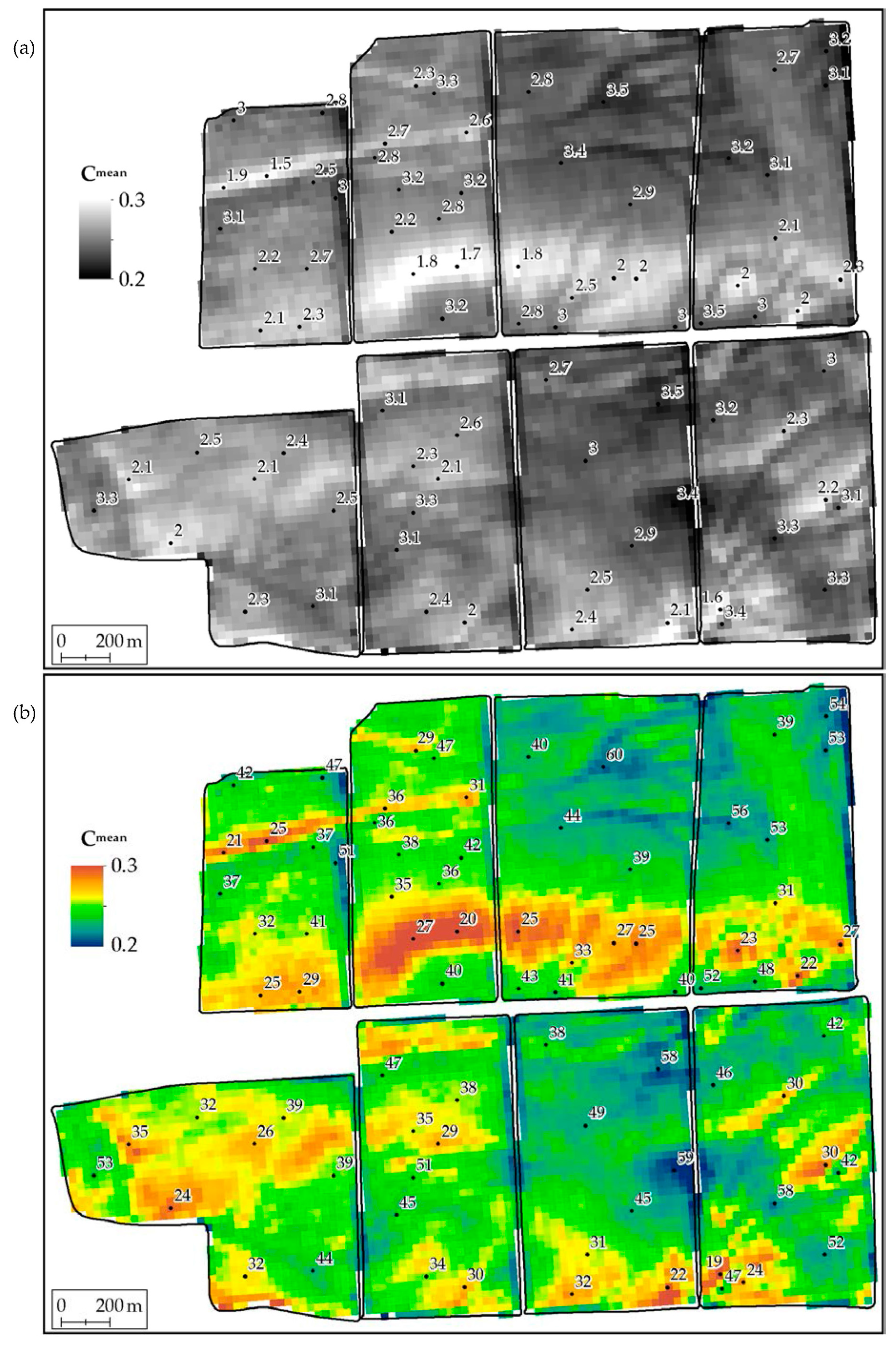
9.

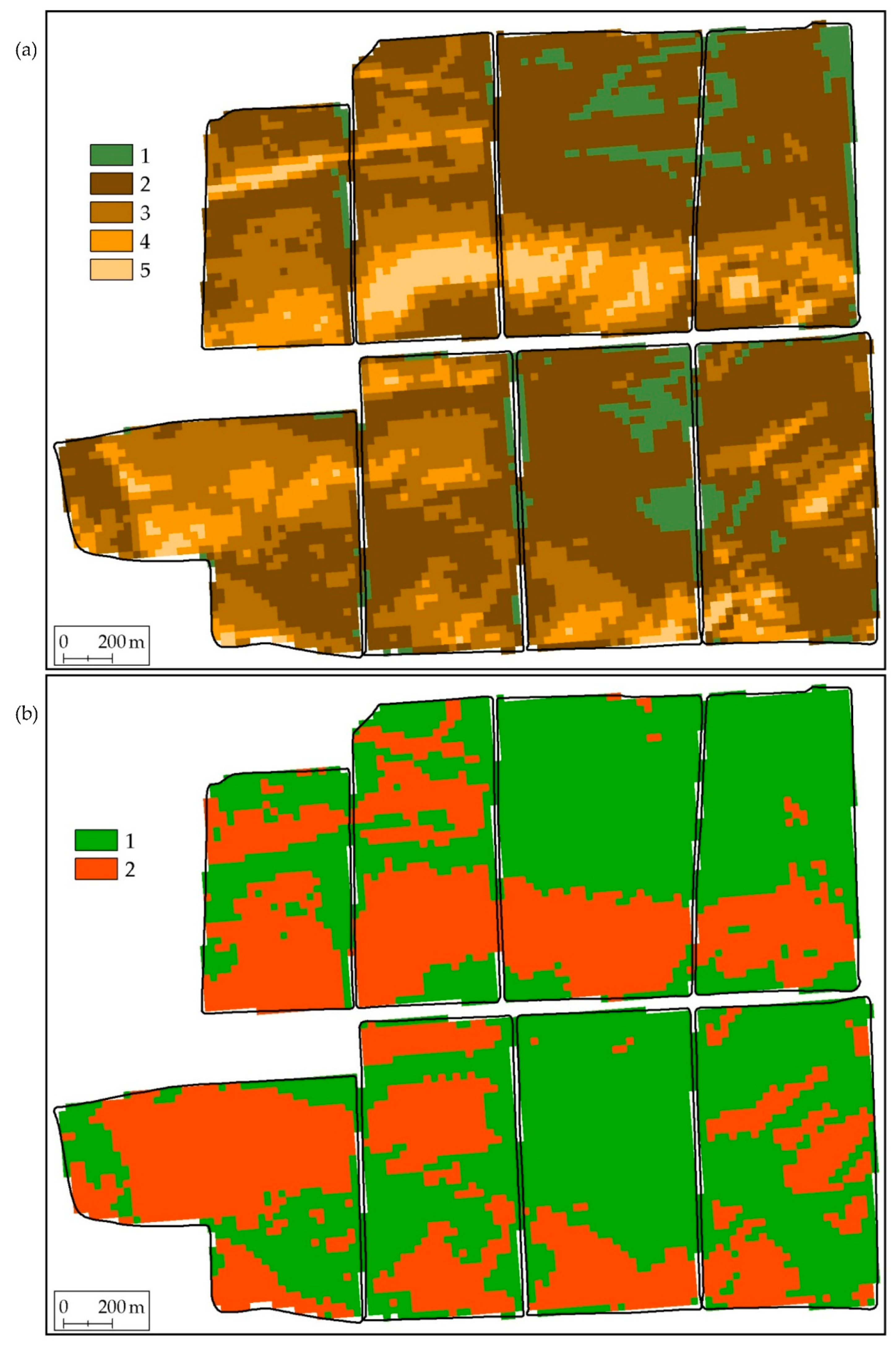
Map of C_mean coefficient values.

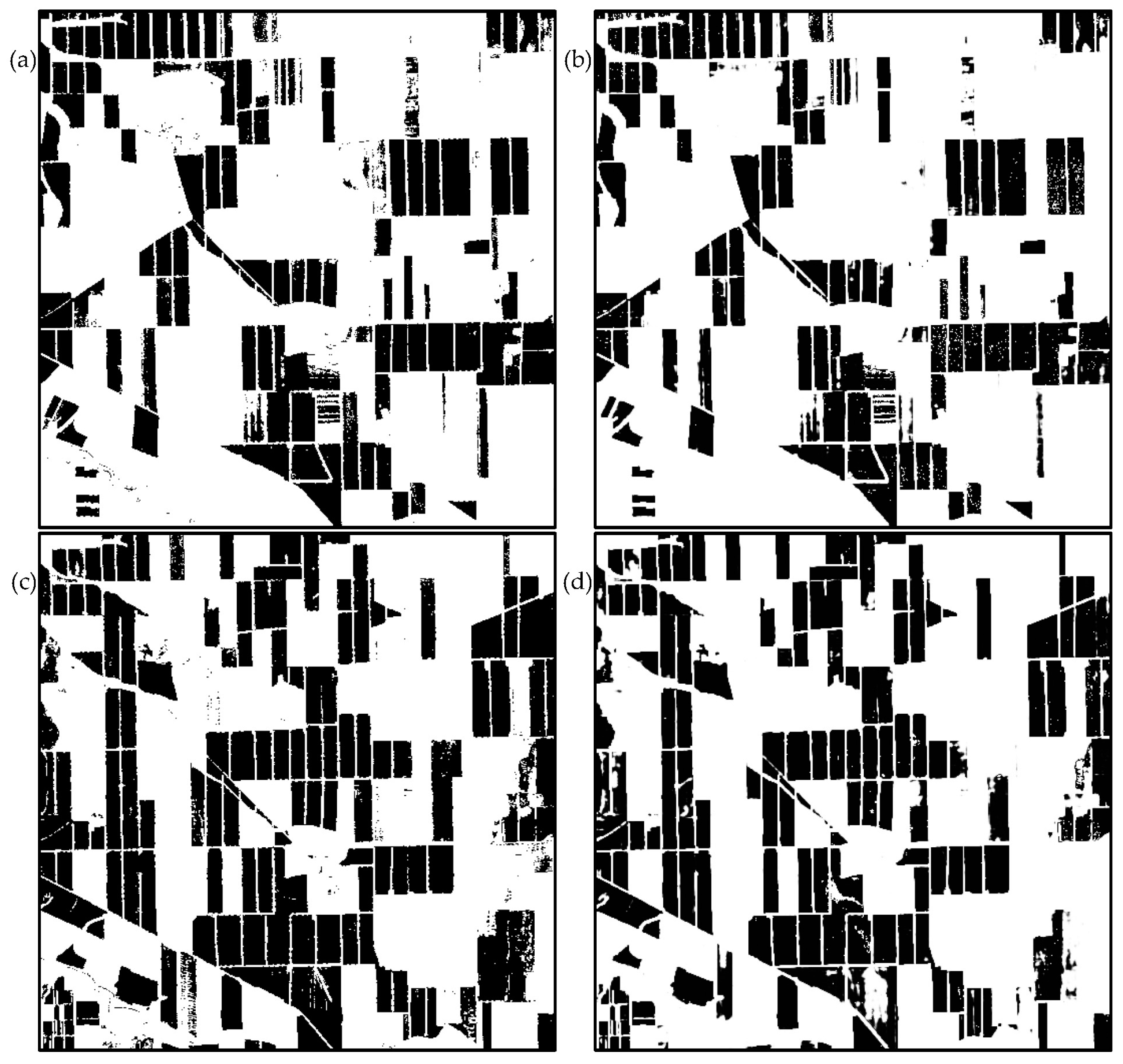
10.

Binary map of the distribution of soil degradation.

11.

Soil map constructed in the result of the classification of the C_mean coefficient.

3.3. Ground Verification and Soil Interpretation of the C_mean Coefficient Map

On the territory of the study, the coefficient C_mean takes values from 0.2 to 0.3 conventional units of the spectral space, i.e., it is a dimensionless coefficient. The values are in the form of a continuous numerical series. In the monochrome color scale, the coefficient C_mean is shown in Figure 8a. Higher ratio values are light, while lower values are dark. More clearly, the spatial distribution of the C_mean coefficient can be represented in the palette from blue to brown tones (Figure 8b). The maps show the results of averaging the spectral brightness over 35 years. Maps are the results of big satellite data processing [27,42]. Machine learning is used in this work for data mining [48,49].

Figure 8a shows the values of the OM content for the soil pits (Table 1). It is easy to note that the lower the values of OM content, the higher the values of C_mean. A graphical representation of the dependence of the OM content on the value of the C_mean coefficient is shown on Figure 9a. The high values of the R² coefficient (0.841) make it possible to interpret the C_mean coefficient map as a map of the OM content in the plow horizon.

From Table 1 and

Table 2. Classification of ranges of the C_mean coefficient according to soil varieties.

Soil Number	Soil Name	Cmean Range
1	meadow-chestnut	0.200–0.220
2	dark chestnut	0.220–0.245
3	dark chestnut slightly eroded	0.245–0.260
4	dark chestnut medium eroded	0.260–0.275
5	dark chestnut strongly eroded	0.275–0.300

, it is also possible to establish the relationship between the names of the soil varieties and the C_mean values. Ground-based methods identified five soil varieties: meadow-chestnut, dark chestnut, dark chestnut slightly eroded, dark chestnut medium eroded and dark chestnut strongly eroded. Each soil variety has its own range of C_mean values (Table 2). Based on empirically determined ranges of C_mean values, a soil map of the study area was constructed. The areas of the soil map obtained by the empirical classification of C_mean were analyzed for statistical significance according to the data of ground studies and the values of C_mean. The C_mean coefficient classification is statistically significant for soil varieties according to the analysis of variance (ANOVA) (Tables S4 and S5). A post hoc analysis of the means according to the Tukey test showed that all soils differ in the thickness of the humus horizon (

Table 3. Post hoc analysis of the means of thickness of humus horizon in soil varieties (significant differences are shown in red).

Soils	Approximate Probabilities (p-Values) for Post Hoc Test *
	1 Mean = 56.857	2 Mean = 44.152	3 Mean = 35.000	4 Mean = 29.769	5 Mean = 24.214
1		0.000124	0.000123	0.000123	0.000123
2	0.000124		0.000125	0.000123	0.000123
3	0.000123	0.000125		0.017242	0.000123
4	0.000123	0.000123	0.017242		0.009697
5	0.000123	0.000123	0.000123	0.009697

* Error: Between groups MS = 17.464, ds = 75.00.

). According to the content of OM, meadow-chestnut and dark chestnut soils, as well as slightly and medium eroded dark chestnut soils, do not differ from each other (

Table 4. Post hoc analysis of the means of OM content in soil varieties (significant differences are shown in red).

Soils	Approximate Probabilities (p-Values) for Post Hoc Test *
	1 Mean = 3.3143	2 Mean = 3.0545	3 Mean = 2.4231	4 Mean = 2.2769	5 Mean = 1.9286
1		0.182848	0.000123	0.000123	0.000123
2	0.182848		0.000123	0.000123	0.000123
3	0.000123	0.000123		0.437679	0.000124
4	0.000123	0.000123	0.437679		0.001194
5	0.000123	0.000123	0.000124	0.001194

* Error: Between groups MS = 0.0478, ds = 75.00.

).

The average OM content for dark chestnut soils in our study is 3.1%, which is in good agreement with the characteristics of this zonal soil—dark chestnut weakly solonetzic clayey and heavy loamy soil on loess-like clays and loams (Haplic Kastanozems) [96]. This soil is characterized by the following values: the thickness of the humus horizon is 40–60 cm and the OM content is 3–4% [97].

A similar relationship is shown by the thickness of the humus horizon and the values of C_mean (Figure 9b). The thickness of the humus horizon also decreases with increasing C_mean values (Table 1). The correlation is also high, and the R² value is 0.86. Thus, the map of the C_mean coefficient can also be interpreted as a map of the thickness of the humus horizon.

The high correlation of the C_mean coefficient values with the thickness of the humus horizon and the content of OM in the plow horizon is quite logical for the object of study (Figure 10). Indeed, with the development of erosion processes, the thickness of the humus horizon decreases due to the upper, most humus horizons. Horizons containing less humus appear on the surface. The correlation between the thickness of the humus horizon and the content of OM is high—R² is 0.824.

The accuracy of the thematic interpretation of the C_mean calculated from big satellite data can be analyzed in terms of information theory. It is possible to set the values of errors of the first and second type for five soil varieties. According to information theory, we have type I errors (α errors, false positive) and type II errors (β errors, false negative). Type I error is a false alarm. In this study, this means that another soil variety fell into the range of C_mean values for one soil variety. Type II error is the omission of the target. In this study, the omission of the target means that the soil variety did not fall within the range of C_mean coefficient values selected for it. Type I and II errors for soil varieties are presented in

Table 5. Type I and II errors for soil varieties identification.

Soils	Total Number of Soil Pits in the Corresponding Interval of Cmean Values	Properly Defined Soil Varieties		Type I Errors (False Alarm)		Type II Errors (Omission of Target)
		(Soil Pits Number)	%	(Soil Pits Number)	%	(Soil Pits Number)	%
1. meadow-chestnut	7	6	85.7	1	14.3	0	0.0
2. dark chestnut	33	26	78.8	7	21.2	2	6.1
3. dark chestnut slightly eroded	13	10	76.9	3	23.1	11	84.6
4. dark chestnut medium eroded	13	9	69.2	4	30.8	4	30.8
5. dark chestnut strongly eroded	14	11	78.6	3	21.4	1	7.1

. It follows from the table that both omission of the target and false alarm are different for different soils. False alarms range from 14.3 to 30.8%. Omission of the target range from 0 to 84.6%. On the whole, according to the soil map based on the ranges of the C_mean coefficient, 62 soil pits out of 80 soil pits fell into their legend classes (the ranges of the values of the C_mean coefficient). The overall accuracy of the map can be determined as 77.5%. The maximum contribution to the error is made by slightly eroded and moderately eroded dark chestnut soils.

It can be considered established (Figure 11a) that the map of the values of the C_mean coefficient of the study area is a soil map with a legend shown in the Table 2.

3.4. Ground Verification of the Degradation Distribution Map

When mapping the soil cover, identifying the zone of distribution of soil cover degradation is one of the most important tasks [2,3,4,5,6,7]. In this work, 3 out of 5 soil varieties characterize the degradation of dark chestnut soil to varying degrees.

The distribution areas of these three soils are characterized by a higher mean long-term spectral brightness over 35 years. Thus, the degradation zone is detected on the basis of big satellite data [27,42]. We emphasize that the degradation area is detected in this work, not on the basis of an analysis of the state of vegetation. Data sifting is carried out in the direction opposite to the previous work [6].

According to the legend for the soil map (Figure 11a), the range of C_mean values for soils with signs of degradation is between 0.245 and 0.30. Figure 11b shows a map of the distribution of soil degradation indicating the location of the ground survey points. Using Table 1 it is possible to calculate the average values of the OM content and the thickness of the humus horizon for degraded and non-degraded soils. The average values of OM content in the upper horizon are 2.2% for eroded soils and 3.1% for non-eroded soils.

These values are in good agreement with the general characteristics of zonal soils for the study area [96,98]. The average thickness of the humus horizon is 29.5 cm for degraded soils and 46.4 cm for non-degraded ones. The thicknesses of the humus horizon also correspond to dark chestnut soils. The content of OM and the thickness of the humus horizon differ statistically significantly for degraded and non-degraded soils (

Table 6. ANOVA of the difference between degraded and non-degraded soils by thickness of humus horizon.

	Sum of Squares	df	Mean Square	F	p-Value	F Crit
Between groups	5678.45	1	5678.45	146.31	1.42 × 10−19	3.96
Within groups	3027.35	78	38.81
Total	8705.80	79

and

Table 7. ANOVA of the difference between degraded and non-degraded soils by OM content.

	Sum of Squares	df	Mean Square	F	p-Value	F Crit
Between groups	16.11	1	16.11	219.31	2.27 × 10−24	3.96
Within groups	5.73	78	0.07
Total	21.84	79

).

Dark chestnut soils clayey and heavy loamy in arable conditions contain 3–4% of OM in plow horizon and a humus horizon thickness is about 40–60 cm [99]. With a lighter particle size distribution, the OM content can decrease to 2.5%. Thus, the degradation threshold for OM content is below 3%, but above 2.5%. In this study, OM content in the upper horizons of less than 2.7% is attributed to degradation. Soils with a thickness of the humus horizon less than 40 cm can be classified as degraded [97].

The accuracy of the binary map of the distribution of degraded soils (Figure 11b) as well as the accuracy of the soil map (Figure 11a) can be described in terms of information theory. In this study false alarm means that non-eroded soils fell into the range of C_mean values for eroded soils. The omission of the target means that the eroded soils fell within the C_mean range for non-eroded soils. Type I and II errors for soil degradation identification are presented in

Table 8. Type I and II errors for soil degradation identification.

Degraded Soils Based on Cmean Value (Soil Pits Number)	Non-Degraded Soils Based on Cmean Value (Soil Pits Number)	Type I Errors (False Alarm)		Type II Errors (Omission of Target)
		(Soil Pits Number)	%	(Soil pits Number)	%
40	40	1	2.5	7	17.5

. It follows from the table that the omission of the target was 17.5%, and the false alarm was 2.5%. In general, according to the map, 8 soil pits out of 80 did not fall into their binary degradation classes. The accuracy of the map reaches 90%.

Consequently, maps of degradation obtained by analyzing big satellite data make it possible to identify the areas of distribution of degraded soils.

4. Discussion

4.1. Sources and Methods for Detecting Soil Degradation

Information about soil degradation should traditionally be included in soil maps. There is a range of soil maps in different scale for the agricultural territory of Russia: 1:10,000–1:25,000 (Figure 12) [97], 1:50,000–100,000 [100], 1:200,000–1:350,000 [101], 1:1,000,000 [102], 1:2,500,000 [103]. For scales 1:10,000–1: 100,000, the 1973 instruction on soil surveys is applied on the territory of Russia [1].

The instruction of 1973 [1] refers to the methods of manual interpretation of large-scale topographic maps (Figure 2c) and orthophotomaps with a spatial resolution better than 1 m (Figure 2e). Further ground surveys are intended to confirm the types and subtypes of soils that are identified by interpretation. This method is very time consuming and not very accurate. The main advantage of the method is the compilation of a very detailed legend for soil maps of the study area. In this study, the legend to the archival soil map (Figure 12) was sufficient for naming the identified objects.

The retrospective monitoring of soil and land cover is also a manual interpretation method. However, this method is based on the analysis of multi-temporal RSD for the period from 1968 to 2022. Retrospective monitoring makes it possible to reveal various types of soil degradation, including in the Rostov region [28,29,30,31,32], where the present work was carried out. The interpretation also involves digital elevation models and topographic maps. But these materials are for reference only. Degraded territories are mapped only if their direct interpretation on RSD is possible. Retrospective monitoring can be considered a method of analysis of big satellite data in manual mode. The method gives high accuracy, but is very laborious.

Erosion modeling allows one to identify areas of degraded land distribution by automated methods [15,16,17,18]. Modeling is a mathematical analogue of erosion identification from topographic maps. The method is based on the analysis of relief parameters (slopes, exposure, catchment area, etc.) [21,22,23,24]. The main disadvantage of modeling is the allocation of potential rather than actual erosion, which do not always coincide [8].

RSD analysis is widely used for mapping the physical and chemical parameters of the soil [30,104]. Determination of land degradation in the form of soil salinity allows to create salt content maps [105] or soil conductivity maps [106]. The disadvantage of the methods is their narrow specialization for one type of degradation.

Machine learning methods often use the same set of morphometric characteristics of the relief and climatic data as the modeling of erosion processes [107,108,109]. The requirements for the quality of the DEM increase with the detail better than the SRTM DEM [26]. Obtaining accurate DEMs is a costly and laborious procedure, which reduces the value of the method. The main drawback remains in the form of mapping potential rather than actual erosion.

Vegetation indices make it possible to develop automated or automatic methods for constructing maps of intra-field heterogeneity of soil fertility [6,7]. Complex and hard-to-reach materials are not required to calculate vegetation indices [35,39,40]. Vegetation indices make it possible to identify zones of soil degradation [36,37,41]. The main disadvantage of mapping intra-field heterogeneity by vegetation indices is the lack of information about the reasons for the formation of heterogeneity [9]. Even the analysis of multi-temporal RSD series [37] will reveal only the presence of vegetation suppression. But even in one field, the suppression of vegetation can be caused by both degradation factors and natural causes.

In our study, the method of mapping the soil cover by the spectral brightness of the bare soil surface was tested. The method is one of direct diagnostic methods. Since the spectral brightness of the bare soil surface depends on its state (mainly moisture), a procedure of averaging of spectral brightness over more than 35 years is proposed. The use of big satellite data made it possible to obtain average spectral characteristics for each Landsat pixel of entire study area of arable land. The averaging results in the form of the C_mean coefficient allow to create a soil map with a legend of 5 soil varieties. Three out of five soil varieties are classified as degraded. The values of the C_mean coefficient showed a high correlation with the content of OM in the upper soil horizon and the thickness of the humus horizon.

Automation of the soil map construction based on the analysis of the bare soil surface was achieved through the use of deep machine learning. The accuracy of the method in our study is 77.5% when constructing a soil map and 90% when compiling a degradation distribution map.

The proposed method is not demanding on the sources of information, which suggests the possibility of its distribution outside the territory of this study.

4.2. Analysis of I and II Type Errors

The construction of a soil map based on the ranges of the C_mean coefficient makes it possible to analyze the causes of I and II type errors. It should be noted that out of 80 soil pits on the map of the distribution of soil degradation, only 8 soil pits did not coincide with the predicted presence/absence of degradation. In 90% of cases, predictions based on multi-temporal spectral characteristics were correct.

The locations of 7 soil pits were predicted as non-degraded soils, but when describing the soil pits, they were assigned to slightly degraded soils. Degradation in these sections was determined by the thickness of the humus horizon less than 40 cm. The OM content in the upper horizon of these soil pits is relatively high and is not a sign of degradation. Since the tested method for diagnosing degradation is based on spectral characteristics, it can be assumed that, with low degradation, the spectral brightness in some cases does not change because of the high values of OM content. Note that the thickness of the humus horizon does not directly affect the spectral characteristics of the soil surface.

Degradation was predicted in one soil pit, whereas degradation was not described in this soil pit during ground survey. In this case, the thickness of the humus horizon and the OM content are close to the degradation/non-degradation threshold: 41 cm and 2.7%, respectively. It is possible that spectral brightness fluctuations occur in the plow horizon at threshold values. It should also be taken into account that the pixel size is 30 × 30 m, and the soil pit is a point object.

The maximum contribution to errors is made by weakly and moderately eroded soils. These soils are characterized by a decrease in the thickness of the humus horizon with a partial preservation of the OM content in the upper horizon. Therefore, the spectral brightness values of these soils are close or intersect.

4.3. Analysis of Previously Compiled Degradation Maps

The most detailed soil information available for the study area at the time of the work is an archival soil map at a scale of 1:25,000 [97] (Figure 12). On the traditional soil map, 6 classes of the legend are allocated for 8 studied fields. Two classes refer to non-degraded soils, four to degraded ones. Thirty-seven soil pits fall on the non-degraded areas of the archival soil map. Of the 37 soil pits, 20 show signs of degradation. The error is 54%. Forty-three soil pits fall on the degraded areas of the traditional soil map. Of the 43 soil pits, 17 have no signs of degradation. The error is 39.5%. On the whole, out of 80 sections on the map, 37 do not have characteristics marked on the traditional soil map. The accuracy of an archival soil map can be determined at 54%.

All soil varieties that are highlighted on the soil map were identified during ground research. With relatively low accuracy, the traditional soil map is of great value as a reference resource.

4.4. Perspective Remote Sensing Data

When identifying promising RSDs for bare soil analysis, consideration should be given to their conformity to Landsat data selection criteria for this study. As shown in this work, Landsat archives can contain more than 1000 scenes per one discretization element of the Earth’s surface with a spatial resolution of 30 × 30 m for 37 years (1984–2022). When training the neural network, 6 spectral bands (Blue, Green, Red, NIR, SWIR1, SWIR2) are involved, which are the same for the entire Landsat archive. There are no complete analogues of Landsat archives. The closest analogue, the Terra ASTER archive, has a significantly shorter time period, since launched in 1999. In addition, the ASTER archive contains fewer scenes for the time period 1999–2022. The Sentinel 2 archive has an even shorter time period.

It can be assumed that at the moment, RSD ASTER and Sentinel 2 data cannot replace Landsat data in the calculations of the long-term average spectral characteristics of the bare soil surface. The main reason is the less of values of spectral characteristics for calculating the long-term averages.

In addition to replacement, the possibility of supplementing the Landsat multi-temporal series with ASTER and Sentinel 2 data should be considered. The spectral characteristics of these RSDs are close to those of Landsat. Spatial resolution is similar (ASTER) or more detailed (Sentinel 2).

The Sentinel 2 data has spectral characteristics similar to Landsat data. Tasseled caps graphs in the RED-NIR spectral space of are almost identical at close dates of surveys. It can be assumed that a neural network trained on Landsat scenes will be able to recognize the bare soil surface on Sentinel 2 tiles. Work in this direction will be carried out in the following studies on the construction of soil maps based on the analysis of multi-temporal spectral characteristics of the bare soil surface.

ASTER data is more difficult to use to supplement Landsat archives. Additional spectral processing is required-calibration with Landsat 4, 5, 7, 8 data. The ASTER archive is relatively small, the development of the ASTER program is not currently planned. Therefore, the use of ASTER is less promising than Sentinel 2.

4.5. Physical Interpretation of Work Technology

The bare surface of each individual soil variety has a different spectral brightness at RSD of different periods and dates of survey. The main reason of BSS spectral brightness variations on RSD is soil moisture. In the RED-NIR spectral plane water bodies are closer to the origin of coordinates than bare soil [13]. As soil moisture increases, its spectral brightness approaches the spectral characteristics of water bodies. As the soil dries out, its spectral brightness increases. In this work, it is assumed that soil moisture has different values over a long period of observations. Along with soil moisture, the spectral brightness of the bare soil surface will also change. For 35 years, on hundreds of images for each RSD pixel, an array of possible spectral brightness values of the bare soil surface is formed (Figure 7a,b) [14].

At equal humidity, the OM content affects the spectral characteristics. More OM areas of the soil are darker than less OM ones. In other words, soils with a high content of OM have a lower spectral brightness than soils with a lower content of OM.

Both parameters (OM and humidity) change independently of each other. Less OM but more moist soil may be darker than more OM but drier soil. That is why soil cover mapping based on one RSD scene may not allow distinguishing one soil from another.

When analyzing big satellite data, the situation changes. The arrays of spectral brightness values for a long period of time are compared. For dark soils, the mean values differ from those for light soils.

It is unlikely for several arable fields to be in the state of bare soil at the same time. This is a consequence of the alternation of crops (crop rotation). Due to crop rotation, it is not possible to analyze the bare soil surface of several agricultural fields using only one RSD image. When analyzing long-term arrays of spectral values for the bare soil surface, the effect of crop rotation is leveled. For each pixel, the number of bare soil surface values is equalized.

Of course, moisture and OM content are not the only factors affecting the spectral brightness of soils. Soil-forming rocks and granulometric composition of soils have a great influence. But within the same parent rock and the same type of particle size distribution, the content of organic matter is the main factor that determines the spectral brightness of the soil. Increased spectral brightness of soil is also an indicator of non-compliance with the rules of soil use, which leads to an increase in losses due to erosion and, as a result, a decrease in soil organic matter [110].

In this study, the conditions for the uniformity of the granulometric composition and parent rocks are met. The long-term average values of the spectral brightness of more OM soils turned out to be lower than those of less OM soils.

The C_mean coefficient as an average long-term indicator of the RED and NIR spectral brightness well characterizes the OM content in the soils of the study area (Figure 9a). Since the OM content and the thickness of the humus horizon simultaneously decrease during soil degradation (Figure 10) [6], the C_mean coefficient also carries information on the thickness of the humus horizon (Figure 9b). Since the thickness of the humus horizon and the content of OM are the main indicators of soil degradation, the C_mean coefficient allows to map soil degradation (Figure 11b).

This is the physical interpretation of the work, the need for interpretation is substantiated in [111]. As a physical interpretation, regression models of calculated indicators from field measurements were used [107,108].

5. Conclusions

An analysis of several works on creating soil degradation maps allowed us to make several assumptions about the ways and possibilities of achieving the aim of this study—to develop a method for detecting degraded areas of arable land in the south of the European part of Russia based on the recognition of bare soil surface on satellite images using deep machine learning methods and methods for calculating average long-term values of the spectral brightness of the bare soil surface. During the study, all assumptions were confirmed. Indeed, maps of the distribution of soil cover degradation can be built on the basis of big remote sensing data without the use of vegetation indices (indicator botany). In calculations, it is sufficient to use the spectral characteristics of the bare soil surface of the RED and NIR bands. The indicator of soil cover degradation was the long-term average spectral characteristics of degraded lands. The identification of bare soil surface on RSD is possible based on the use of convolutional neural networks (deep machine learning). The processing of multi-temporal RSD proved to be effective not only for mapping the distribution of soil cover degradation, but also for constructing soil maps.

A new method for constructing soil maps and maps of the distribution of soil cover degradation has been developed. The method uses deep machine learning and calculation of long-term average spectral characteristics of the open soil surface. The high spectral brightness of the bare soil surface (above the average spectral brightness of the study area) is an indicator of the distribution of degraded soils. The developed method showed a high correlation of the long-term average spectral brightness of the bare soil surface with the OM content (R² = 0.841) and the thickness of the humus horizon (R² = 0.8599). The accuracy of the degradation map is determined by the type I errors (false alarm)-2.5% and the type II errors (omission of target)-17.5%.

In general, according to the map, 8 soil pits out of 80 did not fall into their binary degradation classes. The accuracy of the map reaches 90%. For the soil map, out of 80 sections, 62 sections fell into their legend classes. The overall accuracy of the map can be determined as 77.5%. The maximum contribution to the error is made by slightly eroded and moderately eroded dark chestnut soils. The soil map and the map of degradation distribution were calculated from 133 BSS masks for Landsat scenes over 35 years, obtained on the basis of deep machine learning. The accuracy of predicting the presence of BSS with deep machine learning was 0.79.

In this work, we applied the original technology of selecting the spectral neighborhood of the soil line (SNSL). SNSL assumes that the exposed soil surface in the RED-NIR spectral plane occupies a special elliptical region that cannot be automatically detected based on the vegetation index theory. A neural network was used to automate the selection of an BSS on each RSD scene.

References

1. Ischenko, T.A. (Ed.) All-Union Instruction on Soil Surveys and the Compilation of Large-Scale Soil Land Use Maps; Kolos: Moscow, Russia, 1973. (In Russian) [Google Scholar]
2. Zhang, Y.; Walker, J.P.; Pauwels, V.R.N.; Sadeh, Y. Assimilation of Wheat and Soil States into the APSIM-Wheat Crop Model: A Case Study. Remote Sens. 2022, 14, 65. [Google Scholar] [CrossRef]
3. Qi, G.; Chang, C.; Yang, W.; Gao, P.; Zhao, G. Soil Salinity Inversion in Coastal Corn Planting Areas by the Satellite-UAV-Ground Integration Approach. Remote Sens. 2021, 13, 3100. [Google Scholar] [CrossRef]
4. Romano, E.; Bergonzoli, S.; Pecorella, I.; Bisaglia, C.; De Vita, P. Methodology for the Definition of Durum Wheat Yield Homogeneous Zones by Using Satellite Spectral Indices. Remote Sens. 2021, 13, 2036. [Google Scholar] [CrossRef]
5. Iwahashi, Y.; Ye, R.; Kobayashi, S.; Yagura, K.; Hor, S.; Soben, K.; Homma, K. Quantification of Changes in Rice Production for 2003–2019 with MODIS LAI Data in Pursat Province, Cambodia. Remote Sens. 2021, 13, 1971. [Google Scholar] [CrossRef]
6. Rukhovich, D.I.; Koroleva, P.V.; Rukhovich, D.D.; Kalinina, N.V. The Use of Deep Machine Learning for the Automated Selection of Remote Sensing Data for the Determination of Areas of Arable Land Degradation Processes Distribution. Remote Sens. 2021, 13, 155. [Google Scholar] [CrossRef]
7. Khitrov, N.B.; Rukhovich, D.I.; Koroleva, P.V.; Kalinina, N.V.; Trubnikov, A.V.; Petukhov, D.A.; Kulyanitsa, A.L. A study of the responsiveness of crops to fertilizers by zones of stable intra-field heterogeneity based on big satellite data analysis. Arch. Agron. Soil Sci. 2020, 66, 1963–1975. [Google Scholar] [CrossRef]
8. Kulyanitsa, A.L.; Rukhovich, D.I.; Koroleva, P.V.; Vilchevskaya, E.V.; Kalinina, N.V. Analysis of the informativity of big satellite precision-farming data processing for correcting large-scale soil maps. Eurasian Soil Sci. 2020, 53, 1709–1725. [Google Scholar] [CrossRef]
9. Rukhovich, D.I.; Koroleva, P.V.; Kalinina, N.V.; Vilchevskaya, E.V.; Suleiman, G.A.; Chernousenko, G.I. Detecting Degraded Arable Land on the Basis of Remote Sensing Big Data Analysis. Eurasian Soil Sci. 2021, 54, 161–175. [Google Scholar] [CrossRef]
10. Rukhovich, D.I.; Rukhovich, A.D.; Rukhovich, D.D.; Simakova, M.S.; Kulyanitsa, A.L.; Bryzzhev, A.V.; Koroleva, P.V. The informativeness of coefficients a and b of the soil line for the analysis of remote sensing materials. Eurasian Soil Sci. 2016, 49, 831–845. [Google Scholar] [CrossRef]
11. Rukhovich, D.I.; Rukhovich, A.D.; Rukhovich, D.D.; Simakova, M.S.; Kulyanitsa, A.L.; Bryzzhev, A.V.; Koroleva, P.V. Maps of averaged spectral deviations from soil lines and their comparison with traditional soil maps. Eurasian Soil Sci. 2016, 49, 739–756. [Google Scholar] [CrossRef]
12. Kulyanitsa, A.L.; Rukhovich, A.D.; Rukhovich, D.D.; Koroleva, P.V.; Rukhovich, D.I.; Simakova, M.S. The Application of the Piecewise Linear Approximation to the Spectral Neighborhood of Soil Line for the Analysis of the Quality of Normalization of Remote Sensing Materials. Eurasian Soil Sci. 2017, 50, 387–396. [Google Scholar] [CrossRef]
13. Koroleva, P.V.; Rukhovich, D.I.; Rukhovich, A.D.; Rukhovich, D.D.; Kulyanitsa, A.L.; Trubnikov, A.V.; Kalinina, N.V.; Simakova, M.S. Location of bare soil surface and soil line on the RED–NIR spectral plane. Eurasian Soil Sci. 2017, 50, 1375–1385. [Google Scholar] [CrossRef]
14. Koroleva, P.V.; Rukhovich, D.I.; Rukhovich, A.D.; Rukhovich, D.D.; Kulyanitsa, A.L.; Trubnikov, A.V.; Kalinina, N.V.; Simakova, M.S. Characterization of soil types and subtypes in N-dimensional space of multitemporal (empirical) soil line. Eurasian Soil Sci. 2018, 51, 1021–1033. [Google Scholar] [CrossRef]
15. Farifteh, J.; Van Der Meer, F.; Atzberger, C.; Carranza, E.J.M. Quantitative analysis of salt-affected soil reflectance spectra: A comparison of two adaptive methods (PLSR and ANN). Remote Sens. Environ. 2007, 110, 59–78. [Google Scholar] [CrossRef]
16. Higginbottom, T.P.; Symeonakis, E. Assessing Land Degradation and Desertification Using Vegetation Index Data: Current Frameworks and Future Directions. Remote Sens. 2014, 6, 9552–9575. [Google Scholar] [CrossRef] [Green Version]
17. Ibrahim, Y.Z.; Balzter, H.; Kaduk, J.; Tucker, C.J. Land degradation assessment using residual trend analysis of GIMMS NDVI3g, soil moisture and rainfall in sub-Saharan west Africa from 1982 to 2012. Remote Sens. 2015, 7, 5471–5494. [Google Scholar] [CrossRef] [Green Version]
18. Mendonça-Santos, M.D.L.; Dart, R.O.; Santos, H.G.; Coelho, M.R.; Berbara, R.L.L.; Lumbreras, J.F. Digital Soil Mapping of Topsoil Organic Carbon Content of Rio de Janeiro State, Brazil. In Digital Soil Mapping; Boettinger, J.L., Howell, D.W., Moore, A.C., Hartemink, A.E., Kienast-Brown, S., Eds.; Springer: New York, NY, USA, 2010; pp. 255–266. [Google Scholar] [CrossRef] [Green Version]
19. Romanenkov, V.; Smith, J.; Smith, P.; Sirotenko, O.D.; Rukhovitch, D.I.; Romanenko, I.A. Soil organic carbon dynamics of croplands in European Russia: Estimates from the “model of humus balance”. Reg. Environ. Chang. 2007, 7, 93–104. [Google Scholar] [CrossRef]
20. Rukhovich, D.I.; Koroleva, P.V.; Vilchevskaya, E.V.; Romanenkov, V.; Kolesnikova, L.G. Constructing a spatially-resolved database for modelling soil organic carbon stocks of croplands in European Russia. Reg. Environ. Chang. 2007, 7, 51–61. [Google Scholar] [CrossRef]
21. Glazunov, G.P.; Gendugov, V.M. A full-scale model of wind erosion and its verification. Eurasian Soil Sci. 2003, 36, 216–226. [Google Scholar]
22. Larionov, G.A.; Dobrovol’skaya, N.G.; Krasnov, S.F.; Liu, B.Y. The new equation for the relief factor in statistical models of water erosion. Eurasian Soil Sci. 2003, 36, 1105–1113. [Google Scholar]
23. Maltsev, K.A.; Yermolaev, O.P. Potential Soil Loss from Erosion on Arable Lands in the European Part of Russia. Eurasian Soil Sci. 2019, 52, 1588–1597. [Google Scholar] [CrossRef]
24. Sukhanovskii, Y.P. Rainfall erosion model. Eurasian Soil Sci. 2010, 43, 1036–1046. [Google Scholar] [CrossRef]
25. AShary, P.; Sharaya, L.S.; Mitusov, A.V. Fundamental quantitative methods of land surface analysis. Geoderma 2002, 107, 1–32. [Google Scholar] [CrossRef]
26. SRTM. Available online: http://srtm.csi.cgiar.org (accessed on 21 February 2022).
27. Farm Management. Satellite Big Data: How It Is Changing the Face of Precision Farming. Available online: http://www.farmmanagement.pro/satellite-big-data-how-it-is-changing-the-face-of-precision-farming/ (accessed on 21 February 2022).
28. Koroleva, P.V.; Rukhovich, D.I.; Shapovalov, D.A.; Suleiman, G.A.; Dolinina, E.A. Retrospective Monitoring of Soil Waterlogging on Arable Land of Tambov Oblast in 2018–1968. Eurasian Soil Sci. 2019, 52, 834–852. [Google Scholar] [CrossRef]
29. Rukhovich, D.I.; Simakova, M.S.; Kulyanitsa, A.L.; Bryzzhev, A.V.; Koroleva, P.V.; Kalinina, N.V.; Chernousenko, G.I.; Vil’Chevskaya, E.V.; Dolinina, E.A. The influence of soil salinization on land use changes in azov district of Rostov oblast. Eurasian Soil Sci. 2017, 50, 276–295. [Google Scholar] [CrossRef]
30. Rukhovich, D.I.; Simakova, M.S.; Kulyanitsa, A.L.; Bryzzhev, A.V.; Koroleva, P.V.; Kalinina, N.V.; Chernousenko, G.I.; Vil’Chevskaya, E.V.; Dolinina, E.A.; Rukhovich, S.V. Methodology for Comparing Soil Maps of Different Dates with the Aim to Reveal and Describe Changes in the Soil Cover (By the Example of Soil Salinization Monitoring). Eurasian Soil Sci. 2016, 49, 145–162. [Google Scholar] [CrossRef]
31. Rukhovich, D.I.; Simakova, M.S.; Kulyanitsa, A.L.; Bryzzhev, A.V.; Koroleva, P.V.; Kalinina, N.V.; Vil’Chveskaya, E.V.; Dolinina, E.A.; Rukhovich, S.V. Retrospective analysis of changes in land uses on vertic soils of closed mesodepressions on the Azov plain. Eurasian Soil Sci. 2015, 48, 1050–1075. [Google Scholar] [CrossRef]
32. Rukhovich, D.I.; Simakova, M.S.; Kulyanitsa, A.L.; Bryzzhev, A.V.; Koroleva, P.V.; Kalinina, N.V.; Vil’Chevskaya, E.V.; Dolinina, E.A.; Rukhovich, S.V. Impact of shelterbelts on the fragmentation of erosional networks and local soil waterlogging. Eurasian Soil Sci. 2014, 47, 1086–1099. [Google Scholar] [CrossRef]
33. Bryzzhev, A.V.; Rukhovich, D.I.; Koroleva, P.V.; Kalinina, N.V.; Vilchevskaya, E.V.; Dolinina, E.A.; Rukhovich, S.V. Organization of retrospective monitoring of the soil cover of Rostov oblast. Eurasian Soil Sci. 2015, 48, 1029–1049. [Google Scholar] [CrossRef]
34. Rukhovich, D.I.; Simakova, M.S.; Kulyanitsa, A.L.; Bryzzhev, A.V.; Koroleva, P.V.; Kalinina, N.V.; Vilchevskaya, E.V.; Dolinina, E.A.; Rukhovich, S.V. Analysis of the use of soil maps in the system of retrospective monitoring of the state of lands and soil cover. Pochvovedeniye 2015, 5, 605–625. (In Russian) [Google Scholar]
35. Shapovalov, D.A.; Koroleva, P.V.; Kalinina, N.V.; Rukhovich, D.I.; Suleiman, G.A.; Dolinina, E.A. Differences in Inventories of Waterlogged Territories in Soil Surveys of Different Years and in Land Management Documents. Eurasian Soil Sci. 2020, 53, 294–309. [Google Scholar] [CrossRef]
36. Xu, H.; Hu, X.; Guan, H.; Zhang, B.; Wang, M.; Chen, S.; Chen, M. A Remote Sensing Based Method to Detect Soil Erosion in Forests. Remote. Sens. 2019, 11, 513. [Google Scholar] [CrossRef] [Green Version]
37. Phinzi, K.; Ngetar, N.S. Mapping soil erosion in a quaternary catchment in Eastern Cape using geographic information system and remote sensing. S. Afr. J. Geomat. 2017, 6, 11. [Google Scholar] [CrossRef] [Green Version]
38. Eckert, S.; Hüsler, F.; Liniger, H.; Hodel, E. Trend analysis of MODIS NDVI time series for detecting land degradation and regeneration in Mongolia. J. Arid. Environ. 2015, 113, 16–28. [Google Scholar] [CrossRef]
39. Ayalew, D.A.; Deumlich, D.; Šarapatka, B.; Doktor, D. Quantifying the Sensitivity of NDVI-Based C Factor Estimation and Potential Soil Erosion Prediction using Spaceborne Earth Observation Data. Remote Sens. 2020, 12, 1136. [Google Scholar] [CrossRef] [Green Version]
40. De Carvalho, D.F.; Durigon, V.L.; Antunes, M.A.H.; De Almeida, W.S.; Oliveira, P.T.S. Predicting soil erosion using Rusle and NDVI time series from TM Landsat 5. Pesqui. Agropecu. Bras. 2014, 49, 215–224. [Google Scholar] [CrossRef] [Green Version]
41. Yengoh, G.T.; Dent, D.; Olsson, L.; Tengberg, A.E.; Tucker, C.J. Limits to the Use of NDVI in Land Degradation Assessment. In Use of the Normalized Difference Vegetation Index (NDVI) to Assess Land Degradation at Multiple Scales; Springer Briefs in Environmental Science; Springer: Cham, Switzerland, 2015; pp. 27–30. [Google Scholar] [CrossRef]
42. Huang, Y.; Chen, Z.-X.; Yu, T.; Huang, X.-Z.; Gu, X.-F. Agricultural remote sensing big data: Management and applications. J. Integr. Agric. 2018, 17, 1915–1931. [Google Scholar] [CrossRef]
43. EarthExplorer. Available online: http://earthexplorer.usgs.gov (accessed on 21 February 2022).
44. Zi, Y.; Xie, F.; Jiang, Z. A Cloud Detection Method for Landsat 8 Images Based on PCANet. Remote Sens. 2018, 10, 877. [Google Scholar] [CrossRef] [Green Version]
45. Zeng, X.; Yang, J.; Deng, X.; An, W.; Li, J. Cloud detection of remote sensing images on Landsat-8 by deep learning. In Proceedings of the Tenth International Conference on Digital Image Processing (ICDIP 2018), Shanghai, China, 9 August 2018; p. 108064Y. [Google Scholar] [CrossRef]
46. Mateo-Garcia, G.; Gómez-Chova, L. Convolutional Neural Networks for Cloud Screening: Transfer Learning from Landsat-8 to Proba-V. In Proceedings of the 2018 IEEE International Geoscience and Remote Sensing Symposium, Valencia, Spain, 22–27 July 2018; pp. 2103–2106. [Google Scholar] [CrossRef]
47. Shao, Z.; Pan, Y.; Diao, C.; Cai, J. Cloud Detection in Remote Sensing Images Based on Multiscale Features-Convolutional Neural Network. IEEE Trans. Geosci. Remote Sens. 2019, 57, 4062–4076. [Google Scholar] [CrossRef]
48. Openshaw, S. Geographical Data Mining: Key Design Issues. In Proceedings of the 4th International Conference on GeoComputation, Fredericksburg, VA, USA, 25–28 July 1999; Available online: http://www.geocomputation.org/1999/051/gc_051.htm (accessed on 21 February 2022).
49. Hastie, T.J.; Tibshirani, R.; Friedman, J.H. The Elements of Statistical Learning: Data Mining, Inference, and Prediction, 2nd ed.; Springer Series in Statistics; Springer: New York, NY, USA, 2008; p. 763. [Google Scholar]
50. Mo, H.; Sun, H.; Liu, J.; Wei, S. Developing window behavior models for residential buildings using XGBoost algorithm. Energy Build. 2019, 205, 109564. [Google Scholar] [CrossRef]
51. Abdullah, A.Y.M.; Masrur, A.; Adnan, M.S.G.; Al Baky, A.; Hassan, Q.K.; Dewan, A. Spatio-temporal Patterns of Land Use/Land Cover Change in the Heterogeneous Coastal Region of Bangladesh between 1990 and 2017. Remote Sens. 2019, 11, 790. [Google Scholar] [CrossRef] [Green Version]
52. Schneider dos Santos, R. Estimating spatio-temporal air temperature in London (UK) using machine learning and earth observation satellite data. Int. J. Appl. Earth Obs. 2020, 88, 102066. [Google Scholar]
53. Li, W.; Fu, H.; Yu, L.; Cracknell, A. Deep Learning Based Oil Palm Tree Detection and Counting for High-Resolution Remote Sensing Images. Remote Sens. 2016, 9, 22. [Google Scholar] [CrossRef] [Green Version]
54. Baeta, R.; Nogueira, K.; Menotti, D.; Dos Santos, J.A. Learning Deep Features on Multiple Scales for Coffee Crop Recognition. In Proceedings of the 2017 30th SIBGRAPI Conference on Graphics, Patterns and Images (SIBGRAPI), Niteroi, Brazil, 17–20 October 2017; pp. 262–268. [Google Scholar]
55. Guirado, E.; Tabik, S.; Alcaraz-Segura, D.; Cabello, J.; Herrera, F. Deep-learning Versus OBIA for Scattered Shrub Detection with Google Earth Imagery: Ziziphus lotus as Case Study. Remote Sens. 2017, 9, 1220. [Google Scholar] [CrossRef] [Green Version]
56. Kussul, N.; Lavreniuk, M.; Skakun, S.; Shelestov, A. Deep Learning Classification of Land Cover and Crop Types Using Remote Sensing Data. IEEE Geosci. Remote Sens. Lett. 2017, 14, 778–782. [Google Scholar] [CrossRef]
57. Nijhawan, R.; Sharma, H.; Sahni, H.; Batra, A. A Deep Learning Hybrid CNN Framework Approach for Vegetation Cover Mapping Using Deep Features. In Proceedings of the 2017 13th International Conference on Signal-Image Technology & Internet-Based Systems (SITIS), Niteroi, Brazil, 17–20 October 2017; pp. 192–196. [Google Scholar] [CrossRef]
58. Petropoulos, G.P.; Vadrevu, K.; Xanthopoulos, G.; Karantounias, G.; Scholze, M. A Comparison of Spectral Angle Mapper and Artificial Neural Network Classifiers Combined with Landsat TM Imagery Analysis for Obtaining Burnt Area Mapping. Sensors 2010, 10, 1967–1985. [Google Scholar] [CrossRef] [PubMed] [Green Version]
59. Padarian, J.; Minasny, B.; McBratney, A.B. Using deep learning for digital soil mapping. Soil 2019, 5, 79–89. [Google Scholar] [CrossRef] [Green Version]
60. Meng, Q.; Zhang, L.; Xie, Q.; Yao, S.; Chen, X.; Zhang, Y. Combined Use of GF-3 and Landsat-8 Satellite Data for Soil Moisture Retrieval over Agricultural Areas Using Artificial Neural Network. Adv. Meteorol. 2018, 2018, 9315132. [Google Scholar] [CrossRef]
61. Rai, A.K.; Mandal, N.; Singh, A.; Singh, K.K. Landsat 8 OLI Satellite Image Classification using Convolutional Neural Network. Procedia Comput. Sci. 2020, 167, 987–993. [Google Scholar] [CrossRef]
62. Khan, M.S.; Semwal, M.; Sharma, A.; Verma, R.K. An artificial neural network model for estimating Mentha crop biomass yield using Landsat 8 OLI. Precis. Agric. 2020, 21, 18–33. [Google Scholar] [CrossRef]
63. NEXT Farming: Smarte Lösungen für Landwirte. Available online: https://www.nextfarming.de/ (accessed on 21 February 2022).
64. Shapovalov, D.A.; Koroleva, P.V.; Kalinina, N.V.; Vilchevskaya, E.V.; Kulyanitsa, A.L.; Rukhovich, D.I. ASF-index-a map of stable intra-field heterogeneity of soil cover fertility, based on big satellite data for precision agriculture tasks. Mejdunarodnyi Selskohozyaistvennyi J. 2020, 1, 9–15. [Google Scholar]
65. ExactFarming. Available online: https://www.exactfarming.com/ru/ (accessed on 21 February 2022).
66. Farmers Edge. Available online: https://www.farmersedge.ca/ru/ (accessed on 21 February 2022).
67. Cropio. Available online: https://about.cropio.com/ru/ (accessed on 21 February 2022).
68. Intterra. Available online: https://intterra.ru/ru (accessed on 21 February 2022).
69. AGRO-SAT Consulting GmbH. Available online: http://agro-sat.de/ (accessed on 21 February 2022).
70. Agronote. Available online: https://www.avgust.com/newspaper/topics/detail.php?ID=6860 (accessed on 21 February 2022).
71. Unified Interdepartmental Information and Statistical System. State Statistics. Available online: https://fedstat.ru/indicator/31328 (accessed on 21 February 2022).
72. Rukhovich, D.I.; Koroleva, P.V.; Vilchevskaya, E.V.; Kalinina, N.V. Digital thematic cartography as a change in the available primary sources and ways of using them. In Digital Soil Mapping: Theoretical and Experimental Studies; Ivanov, A.L., Sorokina, N.P., Savin, I.Y., Eds.; Dokuchaev Soil Science Institute: Moscow, Russia, 2012; pp. 58–86. [Google Scholar]
73. USGS EROS Archive-Declassified Data-Declassified Satellite Imagery-1. Available online: https://www.usgs.gov/centers/eros/science/usgs-eros-archive-declassified-data-declassified-satellite-imagery-1?qt-science_center_objects=0#qt-science_center_objects (accessed on 21 February 2022).
74. Kauth, R.J.; Thomas, G.S. The tasseled cap—A graphic description of the spectral-temporal development of agricultural crops as seen by LANDSAT. In Proceedings of the Symposium on Machine Processing of Remotely Sensed Data, West Lafayette, IN, USA, 29 June–1 July 1976; (A77-15051 04-43). Institute of Electrical and Electronics Engineers, Inc.: New York City, NY, USA, 1976; pp. 4B-41–4B-51. [Google Scholar]
75. McCarty, J.L.; Ellicott, E.A.; Romanenkov, V.; Rukhovitch, D.; Koroleva, P. Multi-year black carbon emissions from cropland burning in the Russian Federation. Atmos. Environ. 2012, 63, 223–238. [Google Scholar] [CrossRef]
76. Rouse, J.W.; Haas, R.H.; Schell, J.A.; Deering, D.W. Monitoring vegetation systems in the great plains with ERTS. In Proceedings of the Third ERTS Symposium, Washington, DC, USA, 10–14 December 1973; Scientific and Technical Information Office, NASA: Washington, DC, USA, 1974; Volume 1, pp. 309–317. [Google Scholar]
77. Kohavi, R. A study of cross-validation and bootstrap for accuracy estimation and model selection. In Proceedings of the 14th International Joint Conference on Artificial Intelligence-Volume 2 (IJCAI’95), Montreal, QC, Canada, 20–25 August 1995; pp. 1137–1143. [Google Scholar]
78. Mullin, M.; Sukthankar, R. Complete Cross-Validation for Nearest Neighbor Classifiers. In Proceedings of the Seventeenth International Conference on Machine Learning (ICML ’00), Stanford, CA, USA, 29 June–2 July 2000; pp. 639–646. [Google Scholar]
79. Goodfellow, I.; Bengio, Y.; Courville, A. Deep Learning; MIT press: Cambridge, MA, USA, 2016. [Google Scholar]
80. Porzi, L.; Bulò, S.R.; Colovic, A.; Kontschieder, P. Seamless Scene Segmentation. 2019 IEEE/CVF Conference on Computer Vision and Pattern Recognition (CVPR); IEEE: New York, NY, USA, 2019; pp. 8269–8278. [Google Scholar]
81. Ronneberger, O.; Fischer, P.; Brox, T. U-net: Convolutional networks for biomedical image segmentation. In International Conference on Medical Image Computing and Computer-Assisted Intervention; Springer: Cham, Switzerland, 2015; pp. 234–241. [Google Scholar]
82. Zhou, Z.; Rahman Siddiquee, M.M.; Tajbakhsh, N.; Liang, J. UNet++: A Nested U-Net Architecture for Medical Image Segmentation. In Deep Learning in Medical Image Analysis and Multimodal Learning for Clinical Decision Support; Stoyanov, D., Maier-Hein, L., Syeda-Mahmood, T., Taylor, Z., Lu, Z., Madabhushi, A., Nascimento, J.C., Moradi, M., Martel, A., Eds.; DLMIA: 2018, ML-CDS 2018, Lecture Notes in Computer Science; Springer: Cham, Switzerland, 2018; Volume 11045, pp. 3–11. [Google Scholar]
83. Liu, Y.; Zhu, Q.; Cao, F.; Chen, J.; Lu, G. High-Resolution Remote Sensing Image Segmentation Framework Based on Attention Mechanism and Adaptive Weighting. ISPRS Int. J. Geo-Inf. 2021, 10, 241. [Google Scholar] [CrossRef]
84. Zhang, J.; Zhu, H.; Wang, P.; Ling, X. ATT Squeeze U-Net: A Lightweight Network for Forest Fire Detection and Recognition. IEEE Access 2021, 9, 10858–10870. [Google Scholar] [CrossRef]
85. Sa, I.; Popović, M.; Khanna, R.; Chen, Z.; Lottes, P.; Liebisch, F.; Nieto, J.; Stachniss, C.; Walter, A.; Siegwart, R. WeedMap: A Large-Scale Semantic Weed Mapping Framework Using Aerial Multispectral Imaging and Deep Neural Network for Precision Farming. Remote Sens. 2018, 10, 1423. [Google Scholar] [CrossRef] [Green Version]
86. Lottes, P.; Behley, J.; Milioto, A.; Stachniss, C. Fully Convolutional Networks with Sequential Information for Robust Crop and Weed Detection in Precision Farming. IEEE Robot. Autom. Lett. 2018, 3, 2870–2877. [Google Scholar] [CrossRef] [Green Version]
87. Ioffe, S.; Szegedy, C. Batch normalization: Accelerating deep network training by reducing internal covariate shift. arXiv 2015, arXiv:1502.03167v3. [Google Scholar]
88. Jadon, S. A survey of loss functions for semantic segmentation. In Proceedings of the 2020 IEEE Conference on Computational Intelligence in Bioinformatics and Computational Biology (CIBCB), Santiago, Chile, 27–29 October 2020; pp. 1–7. [Google Scholar] [CrossRef]
89. Kingma, D.P.; Ba, J. Adam: A method for stochastic optimization. arXiv 2014, arXiv:1412.6980. Available online: https://arxiv.org/abs/1412.6980 (accessed on 21 February 2022).
90. Arnold, R.; Blume, H.P.; Bockheim, J.; Boyadgiev, T.; Bridges, E.; Brinkman, R.; Broll, G.; Bronger, A.; Constantini, E.; Creutzberg, D.; et al. World Reference Base for Soil Resources: IUSS Working Group WRB; Food and Agriculture Organization of the United Nations Rome: Rome, Italy, 1998. [Google Scholar]
91. State Standard of the USSR 26213-91. Soils. Methods for Determination of Organic Matter. 1993. Available online: http://docs.cntd.ru/document/1200023481 (accessed on 21 February 2022).
92. Walkley, A.J.; Black, I.A. Estimation of soil organic carbon by the chromic acid titration method. Soil Sci. 1934, 37, 29–38. [Google Scholar] [CrossRef]
93. ArcGIS. Available online: https://www.esri.com/ru-ru/arcgis/about-arcgis/overview (accessed on 21 February 2022).
94. Erdas Imagine. Available online: https://www.hexagongeospatial.com/products/power-portfolio/erdas-imagine (accessed on 21 February 2022).
95. Chen, X.; Guo, Z.; Chen, J.; Yang, W.; Yao, Y.; Zhang, C.; Cui, X.; Cao, X. Replacing the Red Band with the Red-SWIR Band (0.74ρred + 0.26ρswir) Can Reduce the Sensitivity of Vegetation Indices to Soil Background. Remote Sens. 2019, 11, 851. [Google Scholar] [CrossRef] [Green Version]
96. Unified State Register of Soil Resources of Russia. Available online: http://egrpr.soil.msu.ru/index.php (accessed on 21 February 2022).
97. Soil Map of the Collective Farm Rodina, Morozovsky District, Rostov Region, Scale 1:25000; VISKHAGI Southern Branch: Novocherkassk, Russia, 1975.
98. Pochvennyi institut imeni V.V. Dokuchaeva; Egorov, V.V. Classification and Diagnostics of Soils of the USSR (Russian Translations Series, 42); U.S. Department of Agriculture, The National Science Foundation: Washington, DC, USA, 1986.
99. National Soil Atlas of the Russian Federation. Available online: https://soil-db.ru/soilatlas/razdel-3-pochvy-rossiyskoy-federacii/kashtanovye-i-temno-kashtanovye-pochvy-kashtanovye-i-temno-kashtanovye-micelyarno-karbonatnye-pochvy (accessed on 21 February 2022).
100. Soil Map of Zernogradsky District, Rostov Region, Scale 1:100000; VISKHAGI Southern Branch: Novocherkassk, Russia, 1972.
101. Tsvylev, E.M. (Ed.) Soil Map of Rostov Region, Scale 1:300 000; GUGK: Moscow, Russia, 1989. [Google Scholar]
102. Rukhovich, D.I.; Koroleva, P.V.; Kalinina, N.V.; Vilchevskaya, E.V.; Simakova, M.S.; Dolinina, E.A.; Rukhovich, S.V. State soil map of the Russian federation: An ArcInfo version. Eurasian Soil Sci. 2013, 46, 225–240. [Google Scholar] [CrossRef]
103. Chernousenko, G.I.; Kalinina, N.V.; Khitrov, N.B.; Pankova, E.I.; Rukhovich, D.I.; Yamnova, I.A.; Novikova, A.F. Quantification of the areas of saline and solonetzic soils in the Ural Federal Region of the Russian Federation. Eurasian Soil Sci. 2011, 44, 367–379. [Google Scholar] [CrossRef]
104. Daliakopoulos, I.; Tsanis, I.; Koutroulis, A.; Kourgialas, N.; Varouchakis, A.; Karatzas, G.; Ritsema, C. The threat of soil salinity: A European scale review. Sci. Total Environ. 2016, 573, 727–739. [Google Scholar] [CrossRef] [PubMed]
105. Li, P.; Wu, J.; Qian, H. Regulation of secondary soil salinization in semi-arid regions: A simulation research in the Nanshantaizi area along the Silk Road, northwest China. Environ. Earth Sci. 2016, 75, 1–12. [Google Scholar] [CrossRef]
106. Nawar, S.; Buddenbaum, H.; Hill, J. Digital Mapping of Soil Properties Using Multivariate Statistical Analysis and ASTER Data in an Arid Region. Remote Sens. 2015, 7, 1181–1205. [Google Scholar] [CrossRef] [Green Version]
107. Cook, K.L. An evaluation of the effectiveness of low-cost UAVs and structure from motion for geomorphic change detection. Geomorphology 2017, 278, 195–208. [Google Scholar] [CrossRef]
108. Rahmati, O.; Tahmasebipour, N.; Haghizadeh, A.; Pourghasemi, H.R.; Feizizadeh, B. Evaluation of different machine learning models for predicting and mapping the susceptibility of gully erosion. Geomorphology 2017, 298, 118–137. [Google Scholar] [CrossRef]
109. Gong, C.; Lei, S.; Bian, Z.; Liu, Y.; Zhang, Z.; Cheng, W. Analysis of the Development of an Erosion Gully in an Open-Pit Coal Mine Dump During a Winter Freeze-Thaw Cycle by Using Low-Cost UAVs. Remote Sens. 2019, 11, 1356. [Google Scholar] [CrossRef] [Green Version]
110. Vieira, A.S.; do Valle Junior, R.F.; Rodrigues, V.S.; da Silva Quinaia, T.L.; Mendes, R.G.; Valera, C.A.; Fernandes, L.F.S.; Pacheco, F.A.L. Estimating water erosion from the brightness index of orbital images: A framework for the prognosis of degraded pastures. Sci. Total Environ. 2021, 776, 146019. [Google Scholar] [CrossRef]
111. Yuan, Q.; Shen, H.; Li, T.; Li, Z.; Li, S.; Jiang, Y.; Xu, H.; Tan, W.; Yang, Q.; Wang, J.; et al. Deep learning in environmental remote sensing: Achievements and challenges. Remote Sens. Environ. 2020, 241, 111716. [Google Scholar] [CrossRef]
Figure 1. Location of machine learning and study areas.
Remotesensing 14 02224 g001
Figure 2. Fields of acceptance sample (black lines) and points and numbers of soil pits location displayed on: (a) high resolution remote sensing data, (b) digital elevation model, (c) topographic map, (d) Sentinel 2 image (2021, band combination 12, 8, 3), (e) orthophotomap (2012).
Remotesensing 14 02224 g002
Figure 3. Distribution of density values on the RED-NIR spectral plane for Landsat scene of June 2007.
Remotesensing 14 02224 g003
Figure 4. The dataset of BSS mask formation. (a,b) Landsat images of August 25 and May 26; (c,d) distribution of density values on the RED-NIR spectral plane with SNSL (black line); (e,f) BSS masks.
Remotesensing 14 02224 g004
Figure 5. (a) The proposed U-Net architecture with 6 downsampling and 5 upsampling blocks; (b) a single downsampling block; (c) a single upsampling block.
Remotesensing 14 02224 g005
Figure 6. Examples of manually constructed (a,c) and corresponding predicted (b,d) bare soil masks for 512 × 512 pixels crops from validation images of different dates (BSS is black).
Remotesensing 14 02224 g006
Figure 7. (a) BSS RED and NIR values for one Landsat data pixel for the period from 1984 to 2020; (b) location of the point of long-term average values of RED and NIR for the bare soil surface.
Remotesensing 14 02224 g007
Figure 8. (a) Cmean values distribution and data on the OM content (%); (b) Cmean values distribution and data on the thickness of the humus horizon (cm).
Remotesensing 14 02224 g008
Figure 9. Correlation of Cmean and (a) the OM content; (b) the thickness of the humus horizon.
Remotesensing 14 02224 g009
Figure 10. Correlation of the OM content and the thickness of the humus horizon.
Remotesensing 14 02224 g010
Figure 11. (a) Soil map based on classification of Cmean values (soils are: 1—meadow-chestnut, 2—dark chestnut, 3—dark chestnut slightly eroded, 4—dark chestnut medium eroded, 5—dark chestnut strongly eroded); (b) Degradation distribution map: 1—non-degraded soils, 2—degraded soils.
Remotesensing 14 02224 g011
Figure 12. Soil map [97] on a scale of 25,000; numbers in circles indicate soil varieties: 2—meadow-chestnut and dark chestnut soils, 3—dark chestnut soils, 7—dark chestnut slightly eroded soils, 9—dark chestnut slightly deflated soils, 10—dark chestnut medium eroded soils, 20—strongly eroded and accumulated soils of gully-ravine network; red lines indicate field boundaries; red dots with numbers are soil pits.
Remotesensing 14 02224 g012