1. Introduction
Unmanned aerial vehicles (UAVs) are increasingly used as a timely, inexpensive, and agile platform for collecting high-resolution remote sensing data for applications in precision agriculture. With the aid of a global positioning system (GPS) and an inertial navigation system (INS) technology, UAVs can be equipped with commercially available, high-resolution multispectral sensors to collect valuable information for vegetation monitoring. This data can then be processed to guide field management decisions, potentially leading to significant environmental and economical benefits. For example, the early detection of weed infestations in aerial imagery enables developing site-specific weed management (SSWM) strategies, which can lead to significant herbicide savings, reduced environmental impact, and increased crop yield.
Enabling UAVs for such applications is an active area of research, relevant for various fields, including remote sensing [
1,
2], precision agriculture [
3,
4,
5], and agricultural robotics [
6,
7,
8] and crop science [
9]. In the past years, accelerating developments in data-driven approaches, such as big data and deep neural networks (DNNs) [
10], have allowed for unprecedented results in tasks of crop/weed segmentation, plant disease detection, yield estimation, and plant phenotyping [
11].
However, most practical applications require maps which both cover large areas (on the order of hectares), while preserving the fine details of the plant distributions. This is a key input for subsequent actions such as weed management. We aim to address this issue by exploiting multispectral orthomosaic maps that are generated by projecting 3D point clouds onto a ground plane, as shown in
Figure 1.
Utilizing orthomosaic maps in precision agriculture presents several advantages. Firstly, it enables representing crop or field properties of a large farm in a quantitative manner (e.g., a metric scale) by making use of georeferenced images. Secondly, all multispectral orthomosaic maps are precisely aligned, which allows for feeding stacked images to a DNN for subsequent classification. Lastly, global radiometric calibration, i.e., illumination and vignette compensation, is performed over all input images, implying that we can achieve consistent reflectance maps.
There are, of course, also difficulties in using orthomosaic maps. The most prominent one is that the map size may be too large to serve as an input to a standard DNN without losing its resolution due to GPU memory limitation, which may obscure important properties for distinguishing vegetation. Despite recent advances in DNNs, it is still challenging to directly input huge orthomosaic maps to standard classifiers. We address this issue by introducing a sliding window technique that operates on a small part of the orthomosaic before placing it back on the map. The contributions and aims of the paper are:
The remainder of this paper is structured as follows.
Section 2 presents the state of the art in dense semantic segmentation, large-scale vegetation detection using UAVs, and applications of DNNs in precision agriculture.
Section 3 describes our training/testing dataset, and details our orthomosaic generation and processing procedures. We present our experimental results and discuss open challenges/limitations in
Section 4 and
Section 5, before concluding in
Section 6.
2. Related Work
The potentialities of UAV based remote sensing have attracted a lot of interest in high-resolution vegetation mapping scenarios not only due to their environmental impact, but also their economical benefits. In this section, we review the state-of-the-art in plant detection and classification using UAVs, followed by dense semantic segmentation variants using DNNs and their applications in precision agriculture.
2.1. Vegetation Detection and Classification Using UAVs
With the aid of rapidly developing fundamental hardware technologies (e.g., sensing, integrated circuit, and battery), software technologies such as machine learning and image processing have played a significant role in remote sensing, agricultural robotics, and precision farming. Among a wide range of agricultural applications, several machine learning techniques have demonstrated remarkable improvements for the task of crop/weed classification in aerial imagery [
13,
14,
15,
16].
Perez-Ortiz et al. [
15] proposed a weed detection system categorizing image patches into distinct crop, weed, and soil classes based on pixel intensities in multispectral images and geometric information about crop rows. Their work evaluates different machine learning algorithms, achieving overall classification accuracies of 75–87%. In a later work, the same authors [
16] used a support vector machine classifier for crop/weed detection in RGB images of sunflower and maize fields. They present a method for both inter-row and intra-row weed detection by exploiting the statistics of pixel intensities, textures, shapes and geometrical information.
Sandino et al. [
17] demonstrated the identification of invasive grasses/vegetation using a decision tree classifier with Red-Green-Blue (RGB) images. Although they employ a rather standard image processing pipeline with traditional handcrafted features, their results show an impressive 95%+ classification accuracy for different species. Gao et al. [
18] investigated weed detection by fusing pixel and object-based image analysis (OBIA) for a Random Forest (RF) classifier, combined with a Hough transform algorithm for maize row detection. With an accuracy of 94.5%, they achieved promising weed mapping results which illustrate the benefit of utilizing prior knowledge of a field set-up (i.e., crop row detection), in a similar way to our previous work [
7]. However, the method was only tested with a small orthomosaic image covering 150 m
2 with a commercial semi-automated OBIA feature extractor. Ana et al. [
1], on the other hand, proposed an automated RF-OBIA algorithm for early stage intra-, and inter-weed mapping applications by combining Digital Surface Models (plant height), orthomosaic images, and RF classification for good feature selection. Based on their results, they also developed site-specific prescription maps, achieving herbicide savings of 69–79% in areas of low infestation. In our previous work by Lottes et al. [
7], we exemplified multi-class crop (sugar beet) and weed classification using an RF classifier on high-resolution aerial RGB images. The high-resolution imagery enables the algorithm to detect details of crops and weeds leading to the extraction of useful and discriminative features. Through this approach, we achieve a pixel-wise segmentation on the full image resolution with an overall accuracy of 96% for object detection in a crop vs. weed scenario and up to 86% in a crop vs. multiple weed species scenario.
Despite the promising results of the aforementioned studies, it is still challenging to characterize agricultural ecosystems sufficiently well. Agro-ecosystems are often multivariate, complex, and unpredictable using hand-crafted features and conventional machine learning algorithms [
19]. These difficulties arise largely due to local variations caused by differences in environments, soil, and crop and weed species. Recently, there is a paradigm shift towards data-driven approaches with DNNs that can capture a hierarchical representation of input data. These methods demonstrate unprecedented performance improvements for many tasks, including image classification, object detection, and semantic segmentation. In the following section, we focus on semantic segmentation techniques and their applications, as these are more applicable to identify plant species than image classification or object detection algorithms in agricultural environments, where objects’ boundaries are often unclear and ambiguous.
2.2. Dense (Pixel-Wise) Semantic Segmentation Using Deep Neural Networks
The aim of dense semantic segmentation is to generate human-interpretable labels for each pixel in a given image. This fundamental task presents many open challenges. Most existing segmentation approaches rely on convolutional neural networks (CNNs) [
20,
21]. Early CNN-based segmentation approaches typically follow a two-stage pipeline, first selecting region proposals and then training a sub-network to infer a pre-defined label for each proposal [
22]. Recently, the semantic segmentation community has shifted to methods using fully Convolutional Neural Networks (FCNNs) [
23], which can be trained end-to-end and capture rich image information [
20,
24] because they directly estimate pixel-wise segmentation of the image as a whole. However, due to sequential max-pooling and down-sampling operations, FCNN-based approaches are usually limited to low-resolution predictions. Another popular stream in semantic segmentation is the use of an encoder–decoder architecture with skip-connections, e.g., SegNet et al. [
21], as a common building block in networks [
25,
26,
27]. Our previous work presented a SegNet-based network, weedNet [
8], which is capable of producing higher-resolution outputs to avoid coarse downsampled predictions. However, weedNet can only perform segmentation on a single image due to physical Graphics Processing Unit (GPU) memory limitations. Our current work differs in that it can build maps for a much larger field. Although this hardware limitation will be finally resolved in the future with the development of parallel computing technologies, to the authors’ best knowledge, it is difficult to allocate whole orthomosaic maps (including batches, lossless processing) even on state-of-the art GPU machine memory.
In addition to exploring new neural network architectures, applying data augmentation and utilizing synthetic data are worthwhile options for enhancing the capability of a classifier. These technologies often boost up classifier performance with a small training dataset and stabilize a training phase with a good initialization that can lead to a good neural network convergence. Recently, Kemker et al. [
2] presented an impressive study on handling multispectral images with deep learning algorithms. They generated synthetic multispectral images with the corresponding labels for network initialization and evaluated their performance on a new open UAV-based dataset with 18 classes, six bands, and a GSD of 0.047m. Compared to this work, we present a more domain-specific dataset, i.e., it only has three classes but a four-times higher image resolution, a higher number of bands including composite and visual NIR spectral images, and
1.2 times more data (268k/209k spectral pixels).
2.3. Applications of Deep Neural Networks in Precision Agriculture
As reviewed by Carrio et al. [
10] and Kamilaris et al. [
19], the advent of DNNs, especially CNNs, also spurred increasing interest for end-to-end crop/weed classification [
28,
29,
30,
31,
32] to overcome the inflexibility and limitations of traditional handcrafted vision pipelines. In this context, CNNs are applied pixel-wise in a sliding window, seeing only a small patch around a given pixel. Using this principle, Potena et al. [
28] presented a multi-step visual system based on RGB and NIR imagery for crop/weed classification using two different CNN architectures. A shallow network performs vegetation detection before a deeper network further discriminates between crops and weeds. They perform a pixel-wise classification followed by a voting scheme to obtain predictions for connected components in the vegetation mask, reporting an average precision of 98% if the visual appearance has not changed between the training and testing phases. Inspired by the encoder–decoder network, Milioto et al. [
30] use an architecture which combines normal RGB images with background knowledge encoded in additional input channels. Their work focused on real-time crop/weed classification through a lightweight network architecture. Recently, Lottes et al. [
33] proposed an FCNN-based approach with sequential information for robust crop/weed detection. Their motivation was to integrate information about plant arrangement in order to additionally exploit geometric clues. McCool et al. [
31] fine-tuned a large CNN [
34] for the task at hand and attained efficient processing times by compression of the adapted network using a mixture of small, but fast networks, without sacrificing significant classification accuracy. Another noteworthy approach was presented by Mortensen et al. [
29]. They apply a deep CNN for classifying different types of crops to estimate individual biomass amounts. They use RGB images of field plots captured at 3 m above the soil and report an overall accuracy of 80% evaluated on a per-pixel basis.
Most of the studies mentioned were only capable of processing a single RGB image at a time due to GPU memory limitations. In contrast, our approach can handle multi-channel inputs to produce more complete weed maps.
3. Methodologies
This section presents the data collection procedures, training and testing datasets, and methods of generating multispectral orthomosaic reflectance maps. Finally, we discuss our dense semantic segmentation framework for vegetation mapping in aerial imagery.
3.1. Data Collection Procedures
Figure 2 shows sugar beet fields where we performed dataset collection campaigns. For the experiment at ETH Research station sugar beet (
Beta vulgaris) of the variety ‘Samuela’ (KWS Suisse SA, Basel, Switzerland) were sown on 5/April/2017 at 50 cm row distance, 18 cm intra row distance. No fertilizater was applied because the soil available Nitrogen was considered sufficient for this short-term trial to monitor early sugar beet growth. The experiment at Strickhof (N-trial field) was sown on 17/March/2017 with the same sugar beet variety and plant density configuration. Fertilizer application was 103
(92
, 360
, 10 Mg). The fields expressed high weed pressure with large species diversity. Main weeds were
Galinsoga spec., Amaranthus retroflexus, Atriplex spec., Polygonum spec., Gramineae (Echinochloa crus-galli, agropyron and others.). Minor weeds were
Convolvulus arvensis, Stellaria media, Taraxacum spec. etc. The growth stage of sugar beets ranged from 6 to 8 leaf stage at the moment of data collection campaign (5–18/May/2017) and the sizes of crops and weeds exhibited 8–10 cm and 5–10 cm, respectively. The sugar beets on the Rheinbach field were sowed on 18/Aug./2017 and their growth stage were about one month at the moment of data collection (18/Sep./2017). The size of crops and weeds were 15–20 cm and 5–10 cm respectively. The crops were arranged at 50cm row distance, 20 cm intra row distance. The field was only treated once during the post-emergence stage of the crops by mechanical weed control action and thus is affected by high weed pressure.
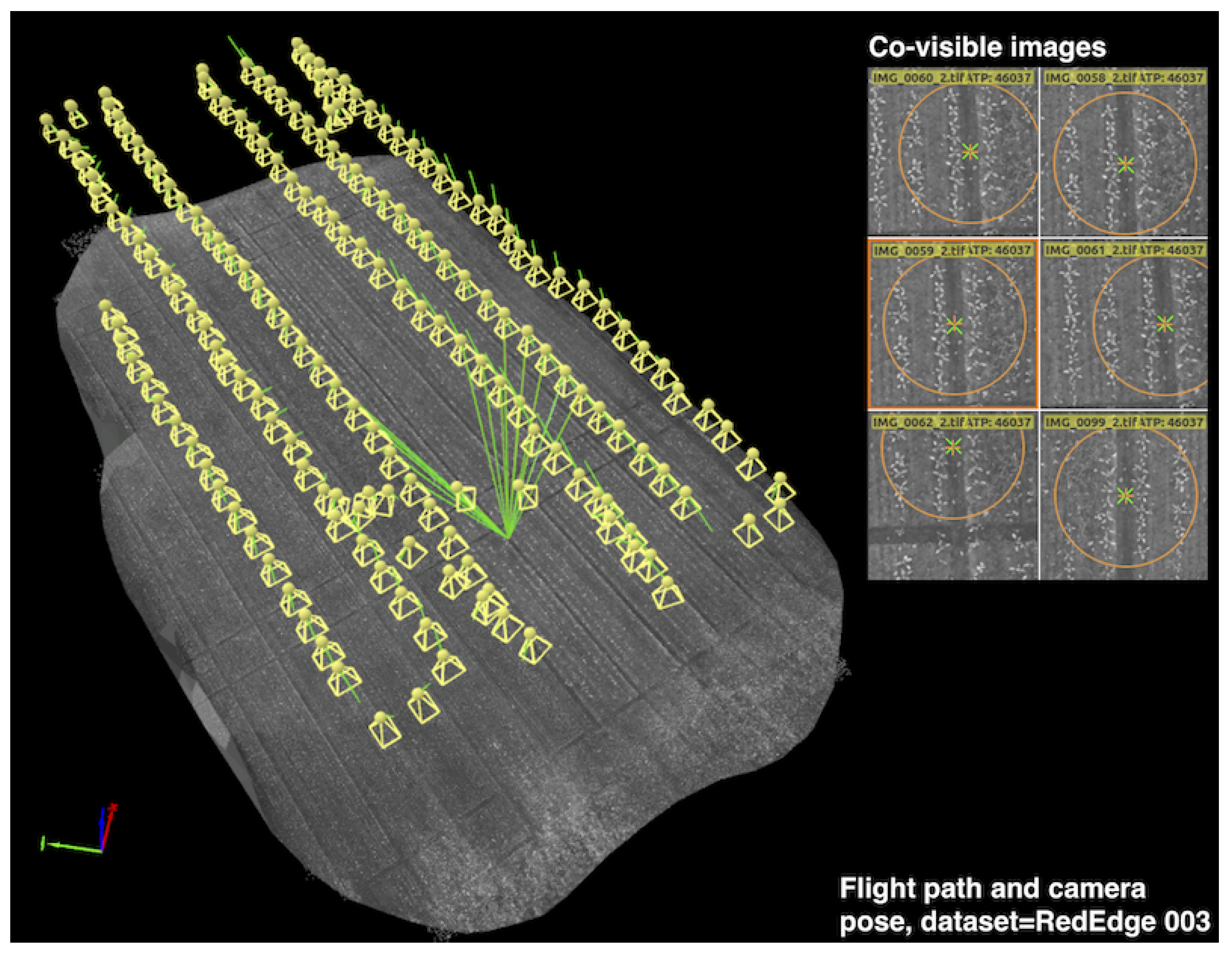
Figure 3 illustrates an example dataset we collected (RedEdge-M 002 from
Table 1, Rheinbach, Germany), indicating the flight path and camera poses where multispectral images were registered. Following this procedure, other datasets were recorded at the same altitude and at similar times of day on different sugar beet fields.
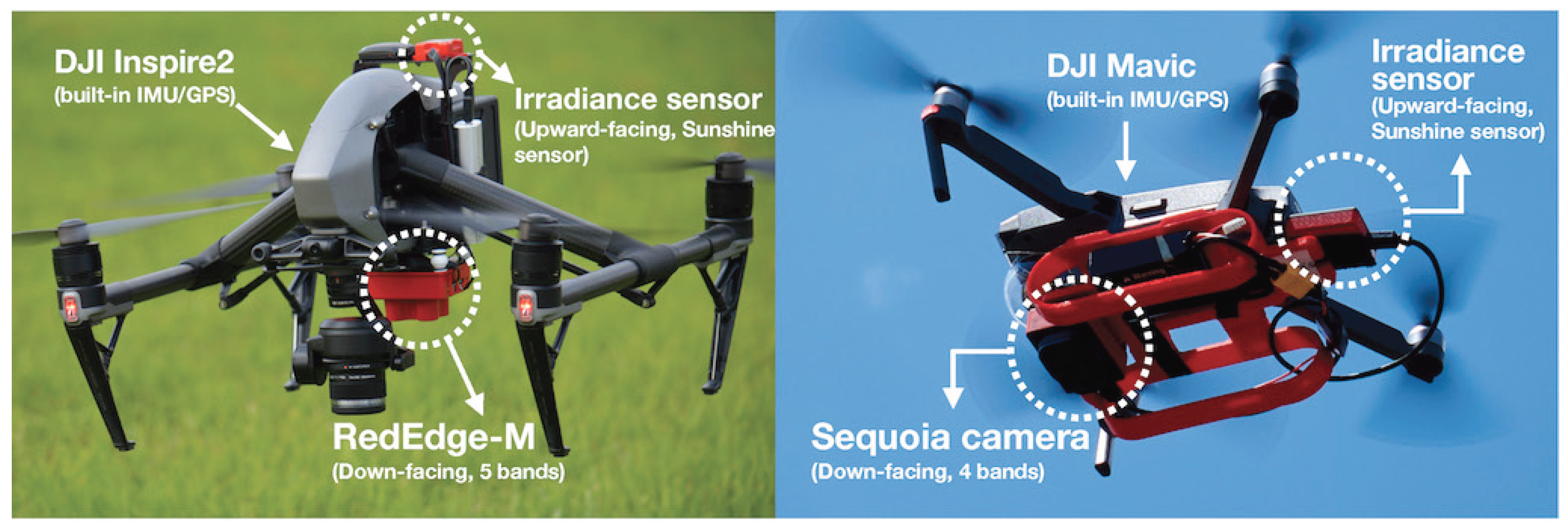
Table 2 details our data collection campaigns. Note that an individual aerial platform shown in
Figure 4 was separately utilized for each sugar beet field.
Table 3 elaborates the multispectral sensor specifications, and
Table 1 and
Table 4 summarize the training and testing datasets for developing our dense semantic segmentation framework in this paper. To assist further research in this area, we make the datasets publicly available [
12].
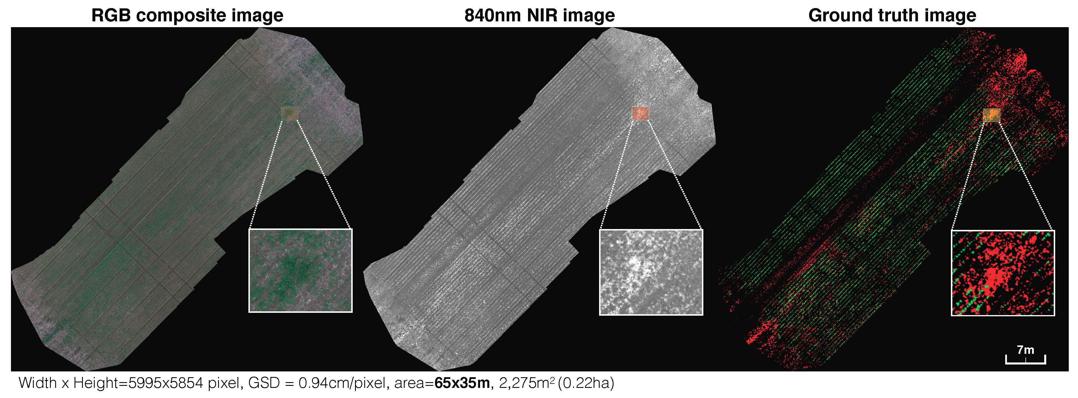
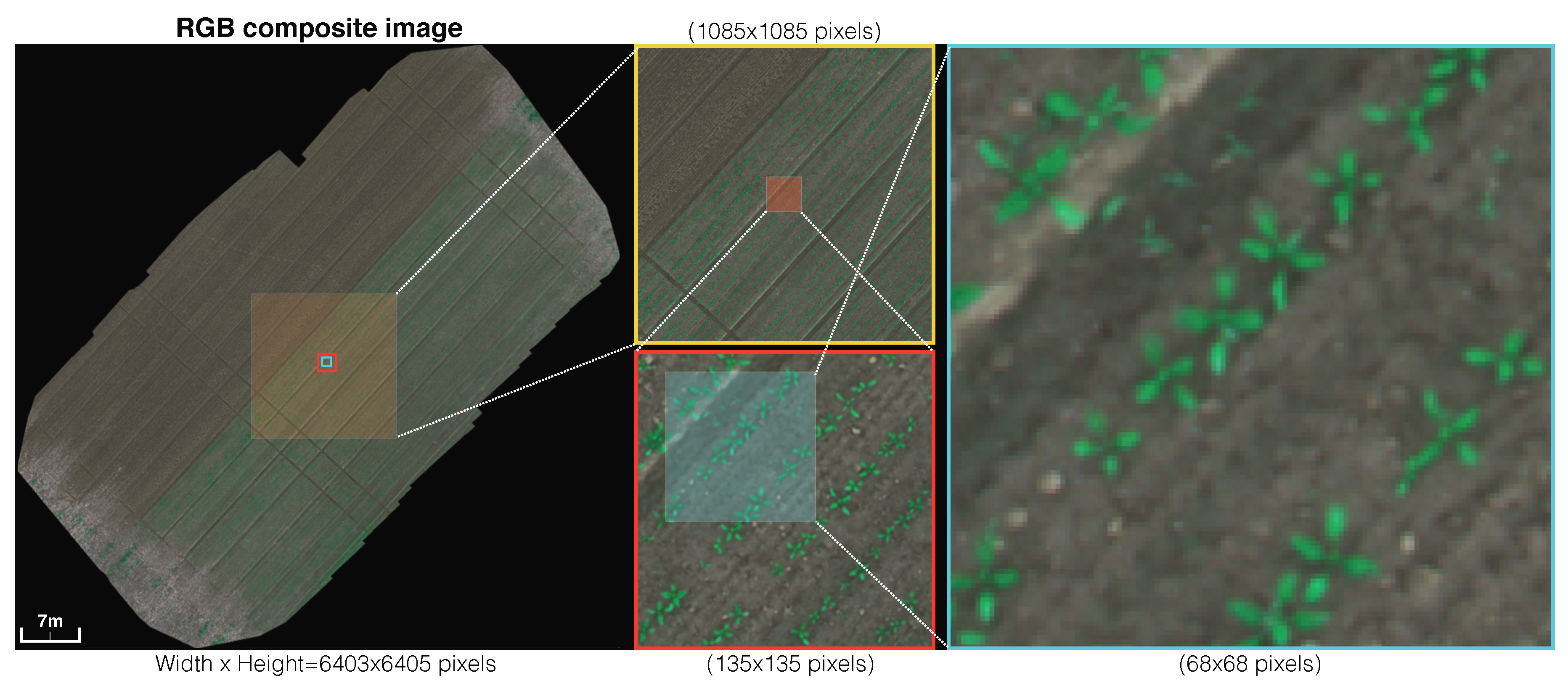
Figure 5 exemplifies the RGB channel of an orthomosaic map generated from data collected with a RedEdge-M camera. The colored boxes in the orthomosaic map indicate areas of different scales on the field, which correspond to varying zoom levels. For example, the cyan box on the far right (68 × 68 pixels) shows a zoomed view of the area within the small cyan box in the orthomosaic map. This figure provides qualitative insight into the high resolution of our map. At the highest zoom level, crop plants are around 15–20 pixels in size and single weeds occupy 5–10 pixels. These clearly demonstrate challenges in crop/weed semantic segmentation due to their small sizes (e.g., 0.05 m weeds and 0.15 m crops) and the visual similarities among vegetation.
As shown in
Table 2, we collected eight multispectral orthomosaic maps using the sensors specified in
Table 3. The two data collection campaigns cover a total area of 1.6554 ha (16,554 m
2). The two cameras we used can capture five and four raw image channels, and we compose them to obtain RGB and color-infrared (CIR) images by stacking the R, G, B channels for an RGB image (RedEdge-M) and R, G, and NIR for a CIR image (Sequoia). We also extract the Normalized Difference Vegetation Index (NDVI) [
35], given by a linear correlation,
. These processes (i.e., color composition for RGB and CIR, and NDVI extraction) result in 12 and eight channels for the RedEdge-M and Sequoia camera, respectively (see
Table 4 for the input data composition). Although some of channels are redundant (e.g., single G channel and G channel from RGB image), they are processed independently with a subsequent convolution network (e.g., three composed pixels from RGB images are convoluted by a kernel that has a different size as that of a single channel). Therefore, we treat each channel as an image, resulting in a total of
1.76 billion pixels composed of 1.39 billion training pixels and 367 million testing pixels (
10,196 images). To our best knowledge, this is the largest publicly available dataset for a sugar beet field containing multispectral images and their pixel-level ground truth.
Table 4 presents an overview of the training and testing folds.
3.2. Training and Testing Datasets
The input image size refers to the resolution of data received by our DNN. Since most CNNs downscale input data due to the difficulties associated with memory management in GPUs, we define the input image size to be the same as that of the input data. This way, we avoid the down-sizing operation, which significantly degrades classification performance by discarding crucial visual information for distinguishing crop and weeds. Note that tile implies that a portion of the region in an image has the same size as that of the input image. We crop multiple tiles from an orthomosaic map by sliding a window over it until the entire map is covered.
Table 1 presents further details regarding our datasets. The Ground Sample Distance (GSD) indicates the distance between two pixel centers when projecting them on the ground given a sensor, pixel size, image resolution, altitude, and camera focal length, as defined by its field of view (FoV). Given the camera specification and flight altitude, we achieved a GSD of around 1 cm. This is in line with the sizes of crops (15–20 pixels) and weeds (5–10 pixels) depicted in
Figure 5.
The number of effective tiles is the number of images actually containing any valid pixel values other than all black pixels. This occurs because orthomosaic maps are diagonally aligned such that the tiles from the most upper left or bottom right corners are entirely black images. The number of tiles in row/col indicates how many tiles (i.e., 480 × 360 images) are composed in a row and column, respectively. Padding information denotes the number of additional black pixels in rows and columns to match the size of the orthomosaic map with a given tile size. For example, the RedEdge-M
000 dataset has a size of 5995 × 5854 for width (column) and height (row), with 245 and 266 pixels appended to the column and row, respectively. This results in a 6240 × 6210 orthomosaic map consisting of 17 row tiles (17 × 360 pixels) and 13 column tiles (13 × 480 pixels). This information is used when generating a segmented orthomosaic map and its corresponding ground truth map from the tiles. For better visualization, we also present the tiling preprocessing method for the RedEdge-M 002 dataset in
Figure 6. The last property, attribute, shows whether the datasets were utilized for training or testing.
3.3. Orthomosaic Reflectance Maps
The output from the orthomosaic tool is the reflectance of each band,
,
where
is the value of the pixel located in the
ith row and
jth column, ordered from top to bottom and left to right in the image, and the top left most pixel is indexed by
i = 0, and
j = 0.
is the reflectance calibration factor of band
k, which can be expressed by [
36]:
where
is the average reflectance of the calibrated reflectance panel (CRP) for the
kth band (
Figure 7), as provided by the manufacturer,
is the radiance for the pixels inside the CRP of the
kth band. The radiance (unit of watt per steradian per square metre per nanometer,
) of a pixel,
, can be written as:
where
are the radiometric calibration coefficients,
is the camera exposure time,
is the sensor gain, and
and
denote the normalized pixel and black level, respectively.
n is the number of bits in the image (e.g.,
n = 12 or 16 bits).
is the 5th order radial vignette model, expressed as:
where
is vignette coefficient, and
r is the distance of the pixel located at (
) from the vignette center (
).
This radiometric calibration procedure is critical to generate a consistent orthomosaic output. We capture two sets of calibration images (before/after) for each data collection campaign, as shown in
Figure 7. To obtain high-quality, uniform orthomosaics (i.e., absolute reflectance), it is important to apply corrections for various lighting conditions such as overcast skies and partial cloud coverage. To correct for this aspect, we utilize sunlight sensors measuring the sun’s orientation and sun irradiance, as shown in
Figure 8.
3.3.1. Orthomosaic Map Generation
Creating orthomosaic images differs to ordinary image stitching as it transforms perspectives to the nadir direction (a top-down view orthogonal to a horizontal plane) and, more importantly, performs true-to-scale operations in which an image pixel corresponds to a metric unit [
37,
38]. This procedure consists of three key steps: (1) initial processing, (2) point densification, and (3) DSM and orthomosaic generation. Step (1) performs keypoints extraction and matching across the input images. A global bundle adjustment method [
39] optimizes the camera parameters, including the intrinsic (distortions, focal length, and principle points) and extrinsic (camera pose) parameters, and triangulated sparse 3D points (structures). Geolocation data such as GPS or ground control points (GCP) are utilized to recover the scale. In Step (2), the 3D points are then densified and filtered [
40]. Finally, Step (3) back-projects the 3D points on a plane to produce 2D orthomosaic images with a nadir view.
Since these orthomosaic images are true to scale (metric), all bands are correctly
aligned. This enables using tiled multispectral images as inputs to the subsequent dense semantic segmentation framework presented in
Section 3.4.
Figure 8 illustrates the entire pipeline implemented in this paper. First, GPS tagged raw multispectral images (five and four channels) are recorded by using two commercial quadrotor UAV platforms which fly over sugar beet fields. Predefined coverage paths at 10m with 80% side and front overlap between consecutive images are passed to the flight controller. The orthomosaic tool [
41] is exploited to generate statistics (e.g., GSD, area coverage, and map uncertainties) and orthomosaic reflectance maps with the calibration patterns presented in
Section 3.3. Based on these reflectance maps, we compose orthomosaic maps, such as RGB, CIR, and NDVI, and tile them as the exact input size for the subsequent dense semantic framework, weedNet [
8], to avoid downscaling. The predictive output containing per-pixel probabilities for each class has the same size as that of the input, and is returned to the original tile location in the orthomosaic map. This methodology is repeated for each tile to ultimately create a large-scale weed map of the target area.
3.4. Dense Semantic Segmentation Framework
In this section, we summarize the dense semantic segmentation framework introduced in our previous work [
8], highlighting only key differences with respect to the original implementation. Although our approach relies on a modified version of the SegNet architecture [
21], it can be easily replaced with any state-of-the-art dense segmentation tool, such as [
26,
30,
42].
3.4.1. Network Architecture
We use the original SegNet architecture in our DNN, i.e., an encoding part with VGG16 layers [
43] in the first half which drops the last two fully-connected layers, followed by upsampling layers for each counterpart in the corresponding encoder layer in the second half. As introduced in [
44], SegNet exploits max-pooling indices from the corresponding encoder layer to perform faster upsampling compared to an FCN [
23].
Our modifications are two-fold. Firstly, the frequency of appearance (FoA) for each class is adapted based on our training dataset for better class balancing [
45]. This is used to weigh each class inside the neural network loss function and requires careful tuning. A class weight can be written as:
where
is the median of
,
is the total number of pixels in class
c, and
is the number of pixels in the
jth image where class
c appears, with
as the image sequence number (
N indicates the total number of images).
In agricultural context, the weed class usually appears less frequently than crop, thus having a comparatively lower FoA. If a false-positive or false-negative is detected in weed classification, i.e., a pixel is incorrectly classified as weed, then the classifier is penalized more for it in comparison to the other classes. We acknowledge that this argument is difficult to generalize to all sugar beet fields, which likely have very different crop/weed ratios compared to our dataset. More specifically, the RedEdge-M dataset has for [background, crop, weed] (hereinafter background referred to as bg) classes with =0.0586 and = [0.9304, 0.0586, 0.0356]. This means that 93% of pixels in the dataset belong to background class, 5.86% is crop, and 3.56% is weed. Sequoia dataset’s is [0.0273, 1.0, 4.3802] with =0.0265 and = [0.9732, 0.0265, 0.0060].
Secondly, we implemented a simple input/output layer that reads images and outputs them to the subsequent concatenation layer. This allows us to feed any number of input channels of an image to the network, which contributes additional information for the classification task [
46].
4. Experimental Results
In this section, we present our experimental setup, followed by our quantitative and qualitative results for crop/weed segmentation. The purpose of these experiments is to investigate the performance of our classifier with datasets varying in input channels and network hyperparameters.
4.1. Experimental Setup
As shown in
Table 1, we have eight multispectral orthomosaic maps with their corresponding manually annotated ground truth labels. We consider three classes,
bg,
crop, and
weed, identified numerically by [0, 1, 2]. In all figures in this paper, they are colorized as [
bg,
crop,
weed].
We used datasets [000, 001, 002, 004] for RedEdge-M (5 channel) training and 003 for testing. Similarly, datasets [006, 007] are used for Sequoia (4 channel) training and 005 for testing. Note that we could not combine all sets for training and testing mainly because their multispectral bands are not matched. Even though some bands of the two cameras overlap (e.g., green, red, red-edge, and NIR), the center wavelength and bandwidth, and the sensor sensitivities vary.
For all model training and experimentation, we used the following hyperparameters: learning rate = 0.001, max. iterations = 40,000, momentum = 9.9, weight decay = 0.0005, and gamma = 1.0. We perform two-fold data augmentation, i.e., the input images are horizontally mirrored.
4.2. Performance Evaluation Metric
For the performance evaluation, we use the area under the curve (AUC) of a precision-recall curve [
47], given by:
where
,
,
,
are the four fundamental numbers, i.e., the numbers of true positive, true negative, false positive, and false negative classifications for class
c. The outputs of the network (480 × 360 × 3) are the probabilities of each pixel belonging to each defined class. For example, the elements [1:480, 1:360, 2] [
48] correspond to pixel-wise probabilities for being
crop. To calculate
,
,
,
, these probabilities should be converted into binary values given a threshold. Since it is often difficult to find the optimal threshold for each class, we exploit
perfcurve [
49] that incrementally varies thresholds from 0 to 1 and computes
,
, and the corresponding AUC. We believe that computing AUC over the probabilistic output can reflect classification performance better than other metrics [
50].
For tasks of dense semantic segmentation, there are many performance evaluation metrics [
44] such as Pixel Accuracy (PA), Mean Pixel Accuracy (MPA), Mean Intersection over Union (MIoU), and Frequency Weighted Intersection over Union (FWIoU). All these metrics either rely on specific thresholds or assign the label with maximum probability among all classes in order to compare individual predictions to ground truth. For instance, a given pixel with a ground truth label of 2 and predictive output label of 3 can be considered a false positive for class 2. However, if a pixel receives probabilistic classifications of 40%, 40%, and 20% for classes 1, 2, and 3, respectively, it may be inappropriate to apply a threshold or choose the maximum probability to determine its predictive output.
4.3. Results Summary
Table 5 displays the dense segmentation results using 20 different models, varying in the number of input channels, batch size, class balance flag, and AUC of each class. Model numbers 1–13 and 14–20 denote the RedEdge-M and Sequoia datasets, respectively. Bold font is used to designate the best scores.
Figure 9 and
Figure 10 show the AUC scores of each class for the RedEdge-M dataset models and their corresponding AUC curves. Analogously,
Figure 11 and
Figure 12 depict the AUC scores for the Sequoia dataset models and their AUC curves. The following sections present a detailed discussion and analysis of these results.
4.3.1. Quantitative Results for the RedEdge-M Dataset
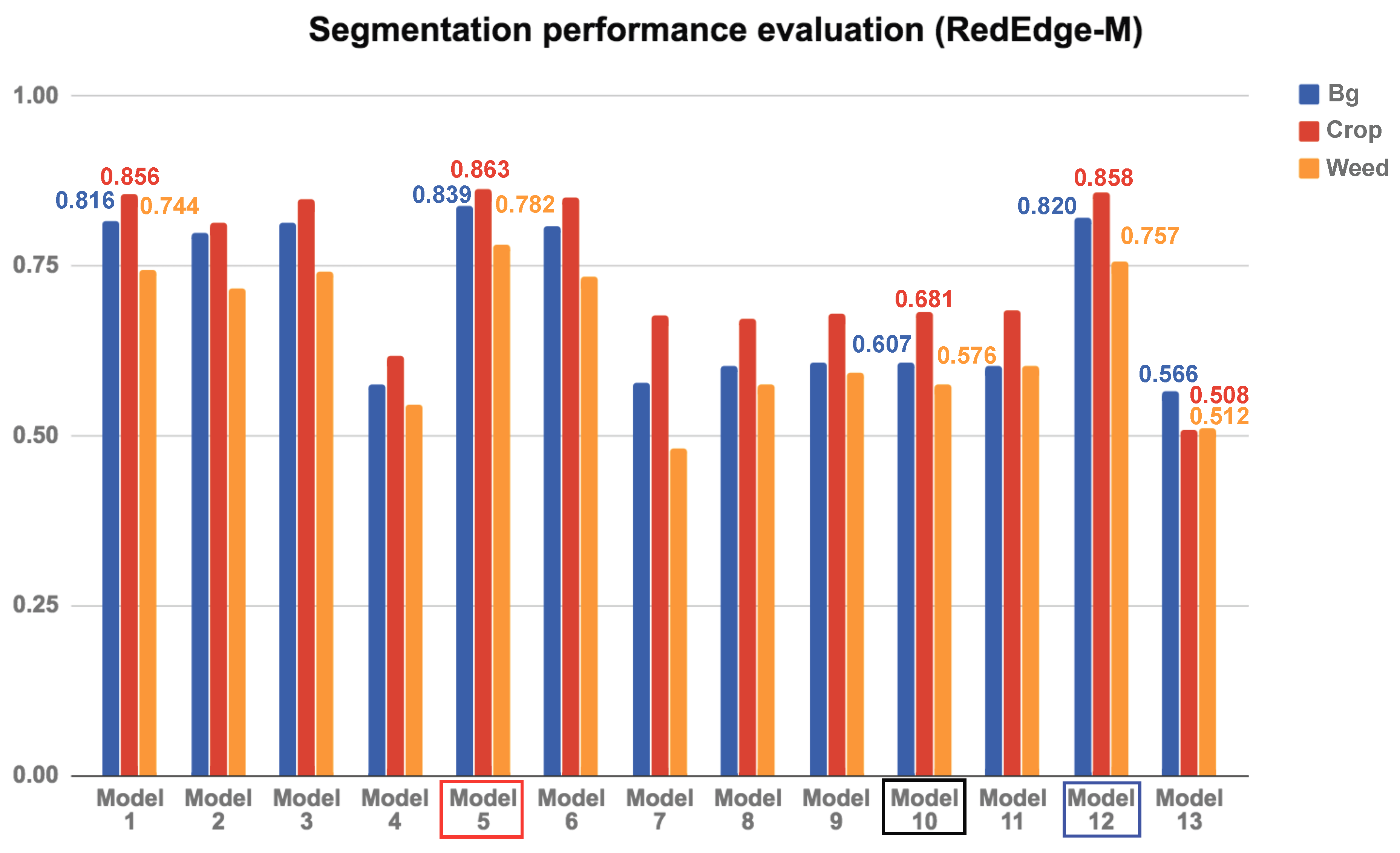
Our initial hypothesis postulated that performance would improve by adding more training data. This argument is generally true, as made evident by Model 10 (our baseline model, the vanilla SegNet with RGB input) and Model 1, but not always; Model 1 and Model 5 present a counter-example. Model 1 makes use of all available input data, but slightly underperforms in comparison to Model 5, which performs best with nine input channels. Although the error margins are small (<2%), this can happen if the RGB channel introduces features that deviate from other features extracted from other channels. As a result, this yields an ambiguity in distinguishing classes and degrades the performance.
Model 1 and Model 2 show the impact of batch size; clearly, increasing the batch size yields better results. The maximum batch size is determined by the memory capacity of the GPU, being six in our case with NVIDIA Titan X (Santa Clara, CA, USA). However, as we often fail to allocate six batches into our GPU memory, we use five batches for most model training procedures apart from the batch size comparison tests.
Model 1 and Model 3 demonstrate the impact of class balancing, as mentioned in
Section 3.4.1.
Model 4 and Model 12 are particularly interesting, because the former excludes only the NDVI channel from the 12 available channels, while the latter uses only this channel. The performance of the two classifiers is very different; Model 12 substantially outperforms Model 4. This happens because the NDVI band already identifies vegetation so that the classifier must only distinguish between crops and weeds. Since the NDVI embodies a linearity between the NIR and R channels, we expect a CNN with NIR and R input channels to perform similarly to Model 12 by learning this relationship. Our results show that the NDVI contributes greatly towards accurate vegetation classification. This suggests that, for a general segmentation task, it is crucial to exploit input information which effectively captures distinguishable features between the target classes.
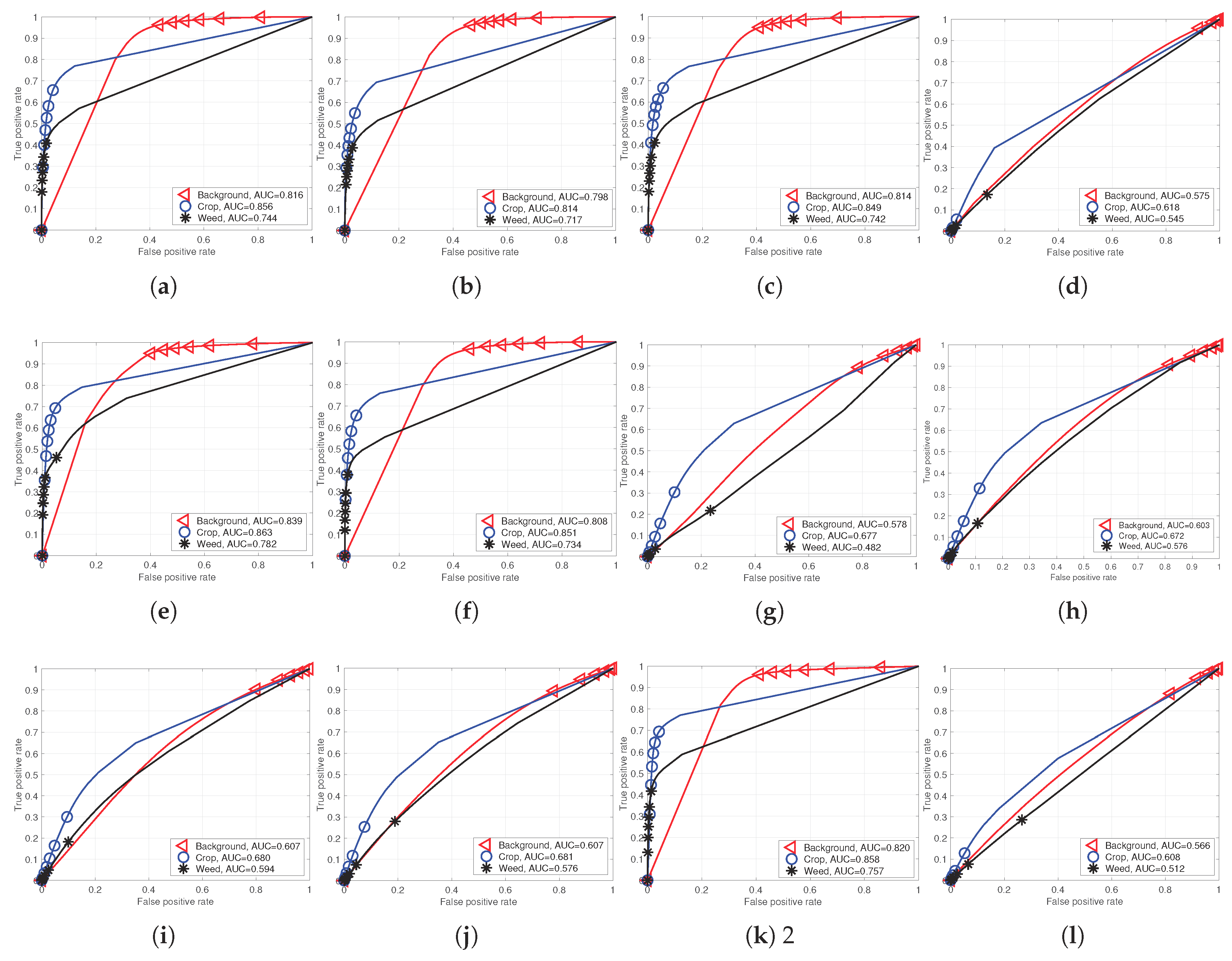
Figure 9 and
Figure 10 show the AUC scores for each model and their performance curves. Note that there are sharp points (e.g., around the 0.15 false positive rate for
crop in
Figure 10c,d). These are points where neither
nor
are changed even with varying thresholds, (
). In this case,
perfcurve generates the point at (1,1) for a monotonic function, enabling AUC to be computed. This rule is equally applied to all other evaluations for a fair comparison, and it is obvious that a better classifier should generate a higher precision and recall point, which, in turn, yields higher AUC even with the linear monotonic function.
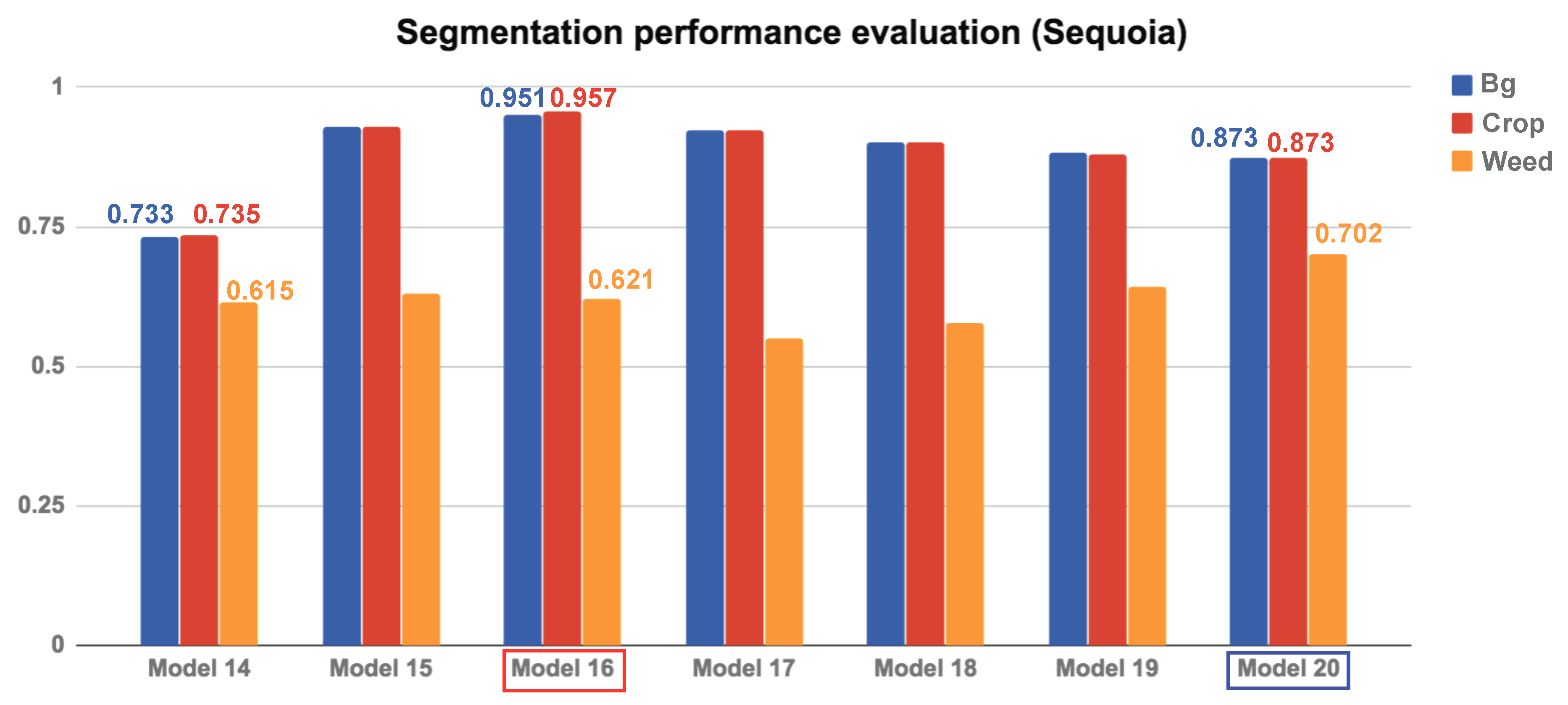
4.3.2. Quantitative Results for the Sequoia Dataset
For the Sequoia dataset, we train seven models with varying conditions. Our results confirm the trends discussed for the RedEdge-M camera in the previous section. Namely, the NDVI plays a significant role in crop/weed detection.
Compared to the RedEdge-M dataset, the most noticeable difference is that the performance gap between crops and weeds is more significant due to their small sizes. As described in
Section 3.1, the crop and weed instances in the RedEdge-M dataset are about 15–20 pixels and 5–10 pixels, respectively. In the Sequoia dataset, they are smaller, as the data collection campaign was carried out at an earlier stage of crop growth. This also reduces weed detection performance (10% worse weed detection), as expected.
In addition, the Sequoia dataset contains 2.6 times less weeds, as per the class weighting ratio described in
Section 3.1 (the RedEdge-M dataset has
for the [
bg,
crop,
weed] classes, while the Sequoia dataset has [0.0273, 1.0, 4.3802]). This is evident by comparing Model 14 and Model 15, as the former significantly outperforms without class balancing. These results are contradictory to those obtained from Model 1 and Model 3 from the RedEdge-M dataset, as Model 1 (with class balancing) slightly outperforms Model 3 (without class balancing). Class balancing can therefore yield both advantages and disadvantages, and its usage should be guided by the datasets and application at hand.
4.4. Qualitative Results
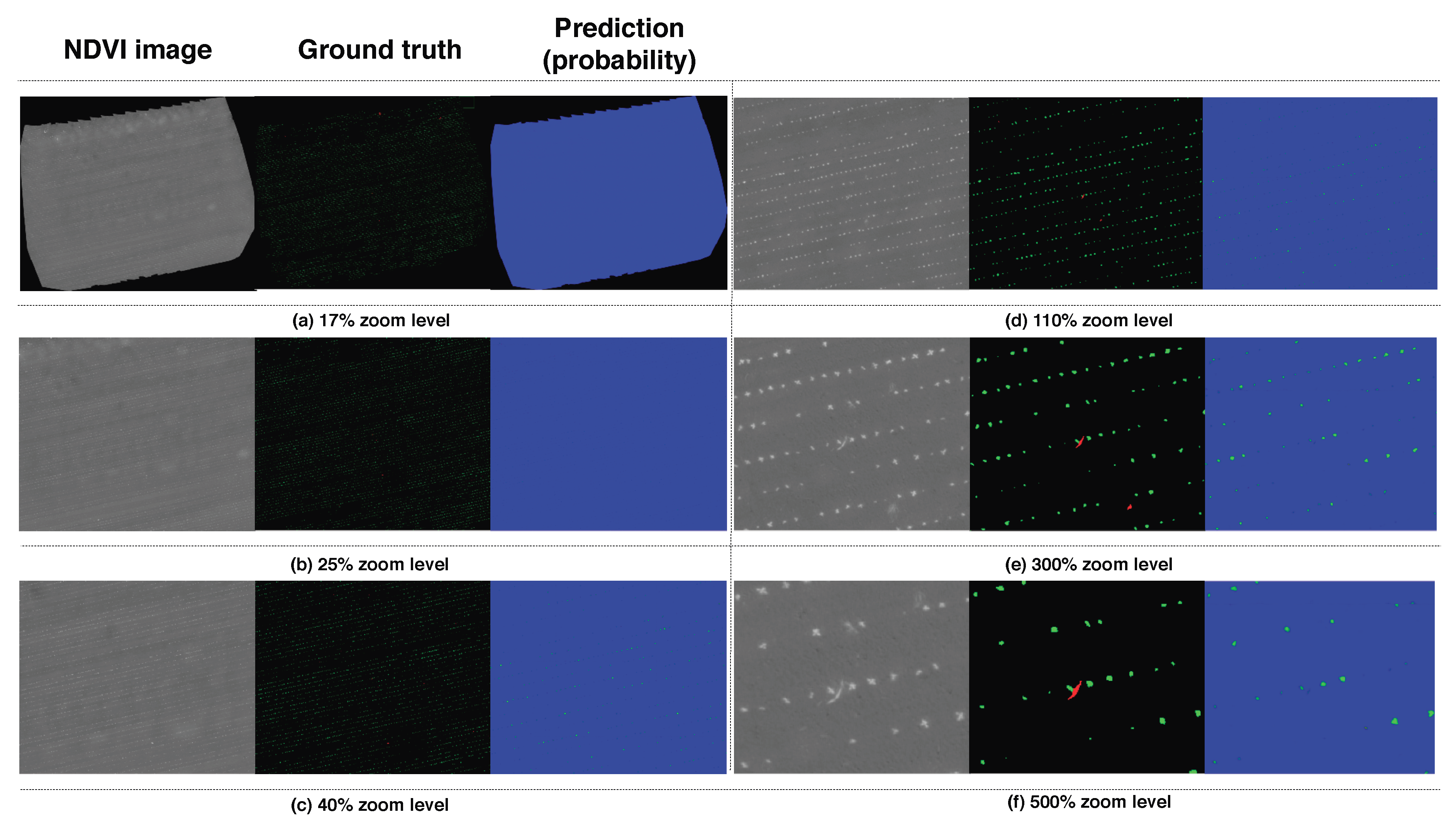
Alongside the quantitative performance evaluation, we also present a qualitative analysis in
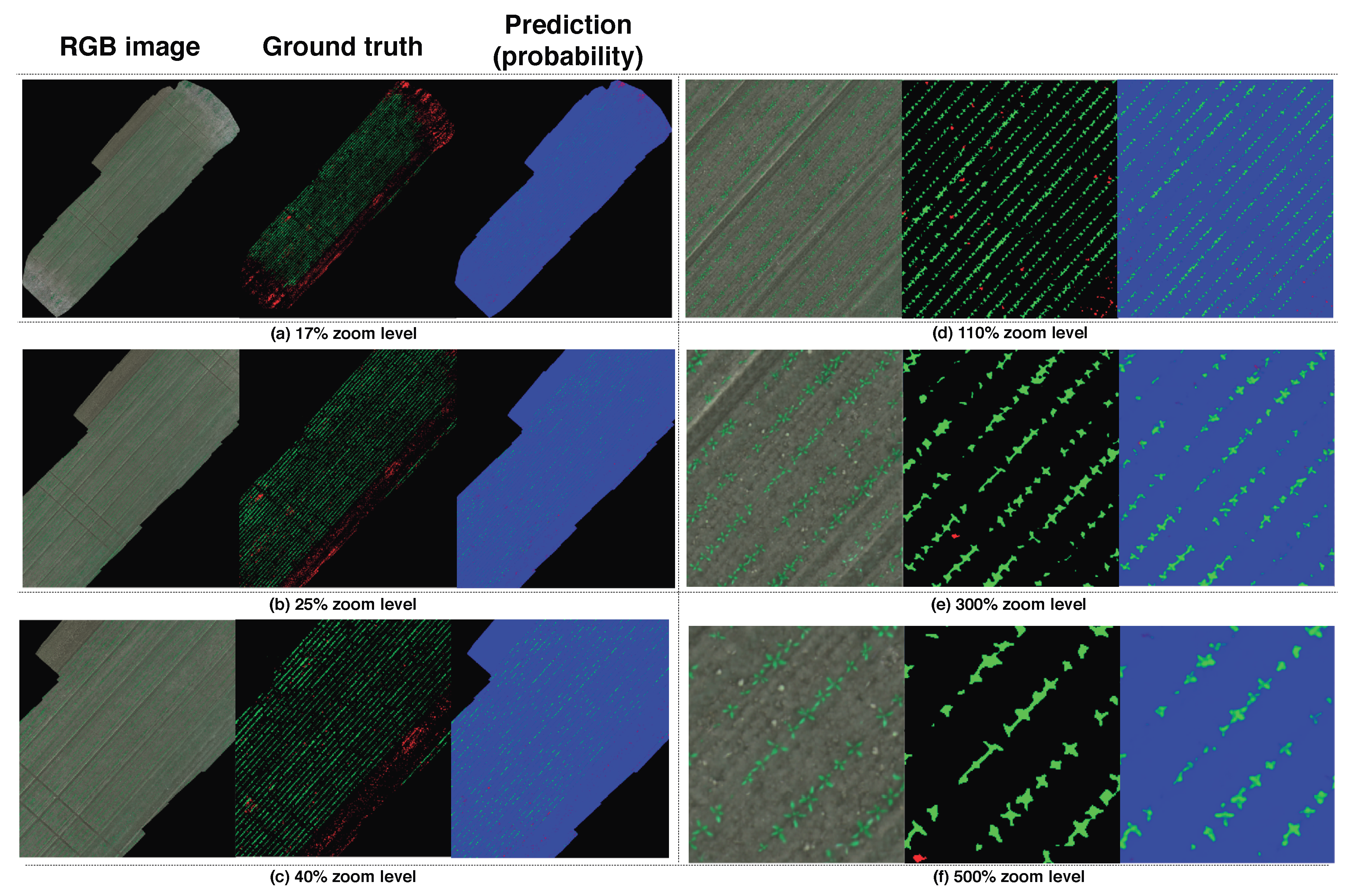
Figure 13 and
Figure 14 for the RedEdge-M and Sequoia testing datasets, i.e., datasets 003 and 005. We use the best performing models (Model 5 for RedEdge-M and Model 16 for Sequoia) that reported AUC of [0.839, 0.863, 0.782] for RedEdge-M and [0.951, 0.957, 0.621] for Sequoia in order to generate the results. As high-resolution images are hard to visualize due to technical limitations such as display or printer resolutions, we display center aligned images with varying zoom levels (17%, 25%, 40%, 110%, 300%, 500%) in
Figure 13a–f. The columns correspond to input images, ground truth images, and the classifier predictions. The color convention follows
bg,
crop,
weed.
4.4.1. RedEdge-M Analysis
In accordance with the quantitative analysis in
Table 5, the classifier performs reasonably for crop prediction.
Figure 13b,c show crop rows clearly, while their magnified views in
Figure 13e,f reveal visually accurate performance at a higher resolution.
Weed classification, however, shows relatively inferior performance in terms of false positives (wrong detections) and false negatives (missing detections) than crop classification. In wider views (e.g.,
Figure 13a–c), it can be seen that the weed distributions and their densities are estimated correctly. The rightmost side, top, and bottom ends of the field are almost entirely occupied by weeds, and prediction reports consistent results with high precision but low recall.
This behavior is likely due to several factors. Most importantly, the weed footprints in the images are too small to distinguish, as exemplified in
Figure 13e,f in the lower left corner. Moreover, the total number of pixels belonging to
weed are relatively smaller than those in
crop, which implies limited weed instances in the training dataset. Lastly, the testing images are unseen as they were recorded in different sugar beet fields than the training examples. This implies that our classifier could be overfitting to the training dataset, or that it learned from insufficient training data for weeds, which only represent a small portion of their characteristics. The higher AUC for crop classification supports this argument, as this class holds less variable attributes across the farm fields.
4.4.2. Sequoia Analysis
The qualitative results for the Sequoia dataset portray similar trends as those of the RedEdge-M dataset, i.e., good crop and relatively poor weed predictions. We make three remarks with respect to the RedEdge-M dataset. Firstly, the footprints of crops and weeds in an image are smaller since data collection was performed at earlier stages of plant growth. Secondly, there was a gap of two weeks between the training (18 May 2017) and testing (5 May 2017) dataset collection, implying a substantial variation in plant size. Lastly, similar to RedEdge-M, the total amount of pixels belonging to the weed class is fewer than those in crop.
5. Discussion on Challenges and Limitations
As shown in the preceding section and our earlier work [
8], obtaining a reliable spatiotemporal model which can incorporate different plant maturity stages and several farm fields remains a challenge. This is because the visual appearance of plants changes significantly during their growth, with particular difficulties in distinguishing between crops and weeds in the early season when they appear similar. High-quality and high-resolution spatiotemporal datasets are required to address this issue. However, while obtaining such data may be feasible for crops, weeds are more difficult to capture representatively due to the diverse range of species which can be found in a single field.
More aggressive data augmentation techniques, such as image scaling and random rotations, in addition to our horizontal flipping procedure, could improve classification performance, as mentioned by [
51,
52]. However, these ideas are only relevant for problems where inter-class variations are large. In our task, applying such methods may be counter-productive as the target classes appear visually similar.
In terms of speed, network forward inferencing takes about 200ms per input image on a NVIDIA Titan X GPU processor, while total map generation depends on the number of tiles in an orthomosaic map. For example, the RedEdge-M testing dataset (003) took 18.8 s (94 × 0.2), while the Sequoia testing dataset (005) took 42 s. Although this process is performed with a traditional desktop computer, it can be accelerated through hardware (e.g., using a state-of-the-art mobile computing device (e.g., NVIDIA Jetson Xavier [
53]) or software improvements (e.g., other network architectures). Note that we omit additional post-processing time from the total map generation, including tile loading and saving the entire weed map, because as these are much faster than the forward prediction step.
The weed map generated can provide useful information for creating prescription maps for the sugar beet field, which can then be transferred to automated machinery, such as fertilizer or herbicide boom sprayers. This procedure allows for minimizing chemical usage and labor cost (i.e., environmental and economical impacts) while maintaining the agricultural productivity of the farm.
6. Conclusions
This paper presented a complete pipeline for semantic weed mapping using multispectral images and a DNN-based classifier. Our dataset consists of multispectral orthomosaic images covering 16,550 m2 sugar beet fields collected by five-band RedEdge-M and four-band Sequoia cameras in Rheinbach (Germany) and Eschikon (Switzerland). Since these images are too large to allocate on a modern GPU machine, we tiled them as the processable size of the DNN without losing their original resolution of ≈1 cm GSD. These tiles are then input to the network sequentially, in a sliding window manner, for crop/weed classification. We demonstrated that this approach allows for generating a complete field map that can be exploited for SSWM.
Through an extensive analysis of the DNN predictions, we obtained insight into classification performance with varying input channels and network hyperparameters. Our best model, trained on nine input channels (AUC of [bg = 0.839, crop = 0.863, weed = 0.782]), significantly outperforms a baseline SegNet architecture with only RGB input (AUC of [0.607, 0.681, 0.576]). In accordance with previous studies, we found that using the NDVI channel significantly helps in discriminating between crops and weeds by segmenting out vegetation in the input images. Simply increasing the size of the DNN training dataset, on the other hand, can introduce more ambiguous information, leading to lower accuracy.
We also introduced spatiotemporal datasets containing high-resolution multispectral sugar beet/weed images with expert labeling. Although the total covered area is relatively small, to our best knowledge, this is the largest multispectral aerial dataset for sugar beet/weed segmentation publicly available. For supervised and data-driven approaches, such as pixel-level semantic classification, high-quality training datasets are essential. However, it is often challenging to manually annotate images without expert advice (e.g., from agronomists), details concerning the sensors used for data acquisition, and well-organized field sites. We hope our work can benefit relevant communities (remote sensing, agricultural robotics, computer vision, machine learning, and precision farming) and enable researchers to take advantage of a high-fidelity annotated dataset for future work. In our work, an unresolved issue is limited segmentation performance for weeds in particular, caused by small sizes of plant instances and their natural variations in shape, size, and appearance. We hope that our work can serve as a benchmark tool for evaluating other crop/weed classifier variants to address the mentioned issues and provide further scientific contributions.
Supplementary Materials
Supplementary File 1Author Contributions
I.S., R.K., P.L., F.L., and A.W. planned and sustained the field experiments; I.S., R.K., and P.L. performed the experiments; I.S. and Z.C. analyzed the data; P.L. and M.P. contributed reagents/materials/analysis tools; C.S., J.N., A.W., and R.S. provided valuable feedback and performed internal reviews. All authors contributed to writing and proofreading the paper.
Funding
This project has received funding from the European Union’s Horizon 2020 research and innovation programme under Grant No. 644227, and the Swiss State Secretariat for Education, Research and Innovation (SERI) under contract number 15.0029.
Acknowledgments
We also gratefully acknowledge the support of NVIDIA Corporation with the donation of the Titan X Pascal GPUs used for this research, Hansueli Zellweger for the management of the experimental field at the ETH plant research station, and Joonho Lee for supporting manual annotation.
Conflicts of Interest
The authors declare no conflict of interest.
Abbreviations
The following abbreviations are used in this manuscript:
| RGB | red, green, and blue |
| UAV | Unmanned Aerial Vehicle |
| DCNN | Deep Convolutional Neural Network |
| CNN | Convolutional Neural Network |
| OBIA | Object-Based Image Analysis |
| RF | Random Forest |
| SSWM | Site-Specific Weed Management |
| DNN | Deep Neural Network |
| GPS | Global Positioning System |
| INS | Inertial Navigation System |
| DSM | Digital Surface Model |
| GCP | Ground Control Point |
| CIR | Color-Infrared |
| NIR | Near-Infrared |
| NDVI | Normalized Difference Vegetation Index |
| GSD | Ground Sample Distance |
| FoV | Field of View |
| GPU | Graphics Processing Unit |
| AUC | Area Under the Curve |
| PA | Pixel Accuracy |
| MPA | Mean Pixel Accuracy |
| MIoU | Mean Intersection over Union |
| FWIoU | Frequency Weighted Intersection over Union |
| TF | True Positive |
| TN | True Negative |
| FP | False Positive |
| FN | False Negative |
References
- De Castro, A.I.; Torres-Sánchez, J.; Peña, J.M.; Jiménez-Brenes, F.M.; Csillik, O.; López-Granados, F. An Automatic Random Forest-OBIA Algorithm for Early Weed Mapping between and within Crop Rows Using UAV Imagery. Remote Sens. 2018, 10, 285. [Google Scholar] [CrossRef]
- Kemker, R.; Salvaggio, C.; Kanan, C. Algorithms for Semantic Segmentation of Multispectral Remote Sensing Imagery using Deep Learning. ISPRS J. Photogramm. Remote Sens. 2018. [Google Scholar] [CrossRef]
- Zhang, C.; Kovacs, J.M. The application of small unmanned aerial systems for precision agriculture: A review. Precis. Agric. 2012, 13, 693–712. [Google Scholar] [CrossRef]
- López-Granados, F. Weed detection for site-specific weed management: Mapping and real-time approaches. Weed Res. 2011, 51, 1–11. [Google Scholar] [CrossRef]
- Walter, A.; Finger, R.; Huber, R.; Buchmann, N. Opinion: Smart farming is key to developing sustainable agriculture. Proc. Natl. Acad. Sci. USA 2017, 114, 6148–6150. [Google Scholar] [CrossRef] [PubMed]
- Detweiler, C.; Ore, J.P.; Anthony, D.; Elbaum, S.; Burgin, A.; Lorenz, A. Bringing Unmanned Aerial Systems Closer to the Environment. Environ. Pract. 2015, 17, 188–200. [Google Scholar] [CrossRef]
- Lottes, P.; Khanna, R.; Pfeifer, J.; Siegwart, R.; Stachniss, C. UAV-based crop and weed classification for smart farming. In Proceedings of the 2017 IEEE International Conference on Robotics and Automation (ICRA), Singapore, 29 May–3 June 2017; pp. 3024–3031. [Google Scholar]
- Sa, I.; Chen, Z.; Popvic, M.; Khanna, R.; Liebisch, F.; Nieto, J.; Siegwart, R. weedNet: Dense Semantic Weed Classification Using Multispectral Images and MAV for Smart Farming. IEEE Robot. Autom. Lett. 2018, 3, 588–595. [Google Scholar] [CrossRef] [Green Version]
- Joalland, S.; Screpanti, C.; Varella, H.V.; Reuther, M.; Schwind, M.; Lang, C.; Walter, A.; Liebisch, F. Aerial and Ground Based Sensing of Tolerance to Beet Cyst Nematode in Sugar Beet. Remote Sens. 2018, 10, 787. [Google Scholar] [CrossRef]
- Carrio, A.; Sampedro, C.; Rodriguez-Ramos, A.; Campoy, P. A Review of Deep Learning Methods and Applications for Unmanned Aerial Vehicles. J. Sens. 2017. [Google Scholar] [CrossRef]
- Pound, M.P.; Atkinson, J.A.; Townsend, A.J.; Wilson, M.H.; Griffiths, M.; Jackson, A.S.; Bulat, A.; Tzimiropoulos, G.; Wells, D.M.; Murchie, E.H.; et al. Deep machine learning provides state-of-the-art performance in image-based plant phenotyping. Gigascience 2017, 6, 1–10. [Google Scholar] [CrossRef] [PubMed] [Green Version]
- Remote Sensing 2018 Weed Map Dataset. Available online: https://goo.gl/ZsgeCV (accessed on 3 September 2018).
- Jose, G.R.F.; Wulfsohn, D.; Rasmussen, J. Sugar beet (Beta vulgaris L.) and thistle (Cirsium arvensis L.) discrimination based on field spectral data. Biosyst. Eng. 2015, 139, 1–15. [Google Scholar]
- Guerrero, J.M.; Pajares, G.; Montalvo, M.; Romeo, J.; Guijarro, M. Support Vector Machines for crop/weeds identification in maize fields. Expert Syst. Appl. 2012, 39, 11149–11155. [Google Scholar] [CrossRef]
- Perez-Ortiz, M.; Peña, J.M.; Gutierrez, P.A.; Torres-Sánchez, J.; Hervás-Martínez, C.; López-Granados, F. A semi-supervised system for weed mapping in sunflower crops using unmanned aerial vehicles and a crop row detection method. Appl. Soft Comput. 2015, 37, 533–544. [Google Scholar] [CrossRef] [Green Version]
- Perez-Ortiz, M.; Peña, J.M.; Gutierrez, P.A.; Torres-Sánchez, J.; Hervás-Martínez, C.; López-Granados, F. Selecting patterns and features for between- and within- crop-row weed mapping using UAV-imagery. Expert Syst. Appl. 2016, 47, 85–94. [Google Scholar] [CrossRef] [Green Version]
- Sandino, J.; Gonzalez, F.; Mengersen, K.; Gaston, K.J. UAVs and Machine Learning Revolutionising Invasive Grass and Vegetation Surveys in Remote Arid Lands. Sensors 2018, 18, 605. [Google Scholar] [CrossRef] [PubMed]
- Gao, J.; Liao, W.; Nuyttens, D.; Lootens, P.; Vangeyte, J.; Pižurica, A.; He, Y.; Pieters, J.G. Fusion of pixel and object-based features for weed mapping using unmanned aerial vehicle imagery. Int. J. Appl. Earth Obs. Geoinf. 2018, 67, 43–53. [Google Scholar] [CrossRef]
- Kamilaris, A.; Prenafeta-Boldú, F.X. Deep learning in agriculture: A survey. Comput. Electron. Agric. 2018, 147, 70–90. [Google Scholar] [CrossRef]
- Chen, L.C.; Papandreou, G.; Kokkinos, I.; Murphy, K.; Yuille, A.L. Deeplab: Semantic image segmentation with deep convolutional nets, atrous convolution, and fully connected crfs. arXiv, 2016; arXiv:1606.00915. [Google Scholar] [CrossRef] [PubMed]
- Badrinarayanan, V.; Kendall, A.; Cipolla, R. SegNet: A Deep Convolutional Encoder-Decoder Architecture for Image Segmentation. IEEE Trans. Pattern Anal. Mach. Intell. 2017, 39, 2481–2495. [Google Scholar] [CrossRef] [PubMed]
- Girshick, R.; Donahue, J.; Darrell, T.; Malik, J. Rich feature hierarchies for accurate object detection and semantic segmentation. In Proceedings of the IEEE Conference on Computer Vision and Pattern Recognition, Columbus, OH, USA, 23–28 June 2014; pp. 580–587. [Google Scholar]
- Long, J.; Shelhamer, E.; Darrell, T. Fully convolutional networks for semantic segmentation. In Proceedings of the IEEE Conference on Computer Vision and Pattern Recognition, Boston, MA, USA, 7–12 June 2015; pp. 3431–3440. [Google Scholar]
- Dai, J.; He, K.; Sun, J. Boxsup: Exploiting bounding boxes to supervise convolutional networks for semantic segmentation. In Proceedings of the IEEE International Conference on Computer Vision, Santiago, Chile, 11–18 December 2015; pp. 1635–1643. [Google Scholar]
- Li, X.; Chen, H.; .Qi, X.; Dou, Q.; Fu, C.; Heng, P.A. H-DenseUNet: Hybrid Densely Connected UNet for Liver and Liver Tumor Segmentation from CT Volumes. arXiv, 2017; arXiv:1709.07330v3. [Google Scholar] [CrossRef] [PubMed]
- Paszke, A.; Chaurasia, A.; Kim, S.; Culurciello, E. ENet: Deep Neural Network Architecture for Real-Time Semantic Segmentation. arXiv, 2016; arXiv:1606.02147. [Google Scholar]
- Ronneberger, O.; Fischer, P.; Brox, T. U-Net: Convolutional Networks for Biomedical Image Segmentation. In Medical Image Computing and Computer-Assisted Intervention; Springer: New York, NY, USA, 2015; Volume 9351, pp. 234–241. [Google Scholar]
- Potena, C.; Nardi, D.; Pretto, A. Fast and Accurate Crop and Weed Identification with Summarized Train Sets for Precision Agriculture. In Proceedings of the International Conference on Intelligent Autonomous Systems, Shanghai, China, 3–7 July 2016. [Google Scholar]
- Mortensen, A.; Dyrmann, M.; Karstoft, H.; Jörgensen, R.N.; Gislum, R. Semantic Segmentation of Mixed Crops using Deep Convolutional Neural Network. In Proceedings of the International Conference on Agricultural Engineering (CIGR), Aarhus, Denmark, 26–29 June 2016. [Google Scholar]
- Milioto, A.; Lottes, P.; Stachniss, C. Real-time Semantic Segmentation of Crop and Weed for Precision Agriculture Robots Leveraging Background Knowledge in CNNs. In Proceedings of the IEEE International Conference on Robotics & Automation (ICRA), Brisbane, Australia, 21–26 May 2018. [Google Scholar]
- McCool, C.; Perez, T.; Upcroft, B. Mixtures of Lightweight Deep Convolutional Neural Networks: Applied to Agricultural Robotics. IEEE Robot. Autom. Lett. 2017. [Google Scholar] [CrossRef]
- Cicco, M.; Potena, C.; Grisetti, G.; Pretto, A. Automatic Model Based Dataset Generation for Fast and Accurate Crop and Weeds Detection. In Proceedings of the IEEE/RSJ International Conference on Intelligent Robots and Systems (IROS), Vancouver, BC, Canada, 24–28 September 2017. [Google Scholar]
- Lottes, P.; Behley, J.; Milioto, A.; Stachniss, C. Fully Convolutional Networks with Sequential Information for Robust Crop and Weed Detection in Precision Farming. IEEE Robot. Autom. Lett. 2018. [Google Scholar] [CrossRef]
- Szegedy, C.; Vanhoucke, V.; Ioffe, S.; Shlens, J.; Wojna, Z. Rethinking the Inception Architecture for Computer Vision. In Proceedings of the IEEE Conference on Computer Vision and Pattern Recognition (CVPR), Las Vegas, NV, USA, 27–30 June 2016; pp. 2818–2826. [Google Scholar]
- Rouse Jr, J.W.; Haas, R.H.; Schell, J.; Deering, D. Monitoring the Vernal Advancement and Retrogradation (Green Wave Effect) of Natural Vegetation; NASA: Washington, DC, USA, 1973. [Google Scholar]
- MicaSense, Use of Calibrated Reflectance Panels For RedEdge Data. Available online: http://goo.gl/EgNwtU (accessed on 3 September 2018).
- Hinzmann, T.; Schönberger, J.L.; Pollefeys, M.; Siegwart, R. Mapping on the Fly: Real-time 3D Dense Reconstruction, Digital Surface Map and Incremental Orthomosaic Generation for Unmanned Aerial Vehicles. In Proceedings of the Field and Service Robotics—Results of the 11th International Conference, Zurich, Switzerland, 12–15 September 2017. [Google Scholar]
- Oettershagen, P.; Stastny, T.; Hinzmann, T.; Rudin, K.; Mantel, T.; Melzer, A.; Wawrzacz, B.; Hitz, G.; Siegwart, R. Robotic technologies for solar-powered UAVs: Fully autonomous updraft-aware aerial sensing for multiday search-and-rescue missions. J. Field Robot. 2017, 35, 612–640. [Google Scholar]
- Snavely, N.; Seitz, S.M.; Szeliski, R. Photo Tourism: Exploring Photo Collections in 3D; ACM Transactions on Graphics (TOG) ACM: New York, NY, USA, 2006; Volume 25, pp. 835–846. [Google Scholar]
- Furukawa, Y.; Ponce, J. Accurate, dense, and robust multiview stereopsis. IEEE Trans. Pattern Anal. Mach. Intell. 2010, 32, 1362–1376. [Google Scholar] [CrossRef] [PubMed]
- Pix4Dmapper Software. Available online: https://pix4d.com (accessed on 3 September 2018).
- Romera, E.; Álvarez, J.M.; Bergasa, L.M.; Arroyo, R. ERFNet: Efficient Residual Factorized ConvNet for Real-Time Semantic Segmentation. IEEE Trans. Intell. Transp. Syst. 2018, 19, 263–272. [Google Scholar] [CrossRef]
- Simonyan, K.; Zisserman, A. Very deep convolutional networks for large-scale image recognition. arXiv, 2014; arXiv:1409.1556. [Google Scholar]
- Garcia-Garcia, A.; Orts-Escolano, S.; Oprea, S.; Villena-Martinez, V.; Garcia-Rodriguez, J. A Review on Deep Learning Techniques Applied to Semantic Segmentation. arXiv, 2017; arXiv:1704.06857. [Google Scholar]
- Eigen, D.; Fergus, R. Predicting depth, surface normals and semantic labels with a common multi-scale convolutional architecture. In Proceedings of the IEEE International Conference on Computer Vision, Santiago, Chile, 11–18 December 2015; pp. 2650–2658. [Google Scholar]
- Khanna, R.; Sa, I.; Nieto, J.; Siegwart, R. On field radiometric calibration for multispectral cameras. In Proceedings of the 2017 IEEE International Conference on Robotics and Automation (ICRA), Singapore, 29 May–3 June 2017; pp. 6503–6509. [Google Scholar]
- Boyd, K.; Eng, K.H.; Page, C.D. Area under the Precision-Recall Curve: Point Estimates and Confidence Intervals. In Machine Learning and Knowledge Discovery in Databases; Springer: Berlin/Heidelberg, Germany, 2013; pp. 451–466. [Google Scholar]
- MATLAB Expression. Available online: https://ch.mathworks.com/help/images/image-coordinate-systems.html (accessed on 3 September 2018).
- MATLAB Perfcurve. Available online: https://mathworks.com/help/stats/perfcurve.html (accessed on 3 September 2018).
- Csurka, G.; Larlus, D.; Perronnin, F.; Meylan, F. What is a good evaluation measure for semantic segmentation? In Proceedings of the 24th BMVC British Machine Vision Conference, Bristol, UK, 9–13 September 2013.
- Wang, J.; Perez, L. The Effectiveness of Data Augmentation in Image Classification Using Deep Learning. arXiv, 2017; arXiv:1712.04621. [Google Scholar]
- Wong, S.C.; Gatt, A.; Stamatescu, V.; McDonnell, M.D. Understanding Data Augmentation for Classification: When to Warp? In Proceedings of the 2016 International Conference on Digital Image Computing: Techniques and Applications (DICTA), Gold Coast, Australia, 30 November–2 December 2016; pp. 1–6. [Google Scholar]
- NVIDIA Jetson Xavier. Available online: https://developer.nvidia.com/jetson-xavier (accessed on 3 September 2018).
Figure 1.
An example of the orthomosaic maps used in this paper. Left, middle and right are RGB (red, green, and blue). composite, near-infrared (NIR) and manually labeled ground truth (crop = green, weed = red) images with their zoomed-in views. We present these images in order to provide an intuition of the scale of the sugar beet field and quality of data used in this paper.
Figure 2.
Sugar beet fields where we collected datasets. Two fields in Eschikon are shown on the left, and one field in Rheinbach is on the right.
Figure 2.
Sugar beet fields where we collected datasets. Two fields in Eschikon are shown on the left, and one field in Rheinbach is on the right.
Figure 3.
An example UAV trajectory covering a 1300 m
2 sugar beet field (RedEdge-M 002 from
Table 1). Each yellow frustum indicates the position where an image is taken, and the green lines are rays between a 3D point and their co-visible multiple views. Qualitatively, it can be seen that the 2D feature points from the right subplots are properly extracted and matched for generating a precise orthomosaic map. A similar coverage-type flight path is used for the collection of our datasets.
Figure 4.
Multispectral cameras and irradiance (Sunshine) sensors’ configuration. Both cameras are facing-down with respect to the drone body and irradiance sensors are facing-up.
Figure 4.
Multispectral cameras and irradiance (Sunshine) sensors’ configuration. Both cameras are facing-down with respect to the drone body and irradiance sensors are facing-up.
Figure 5.
One of the datasets used in this paper. The left image shows the entire orthomosaic map, and the middle and right are subsets of each area at varying zoom levels. The yellow, red, and cyan boxes indicate different areas on the field, corresponding to cropped views. These details clearly provide evidence of the large scale of the farm field and suggest the visual challenges in distinguishing between crops and weeds due to the limited number of pixels and similarities in appearance.
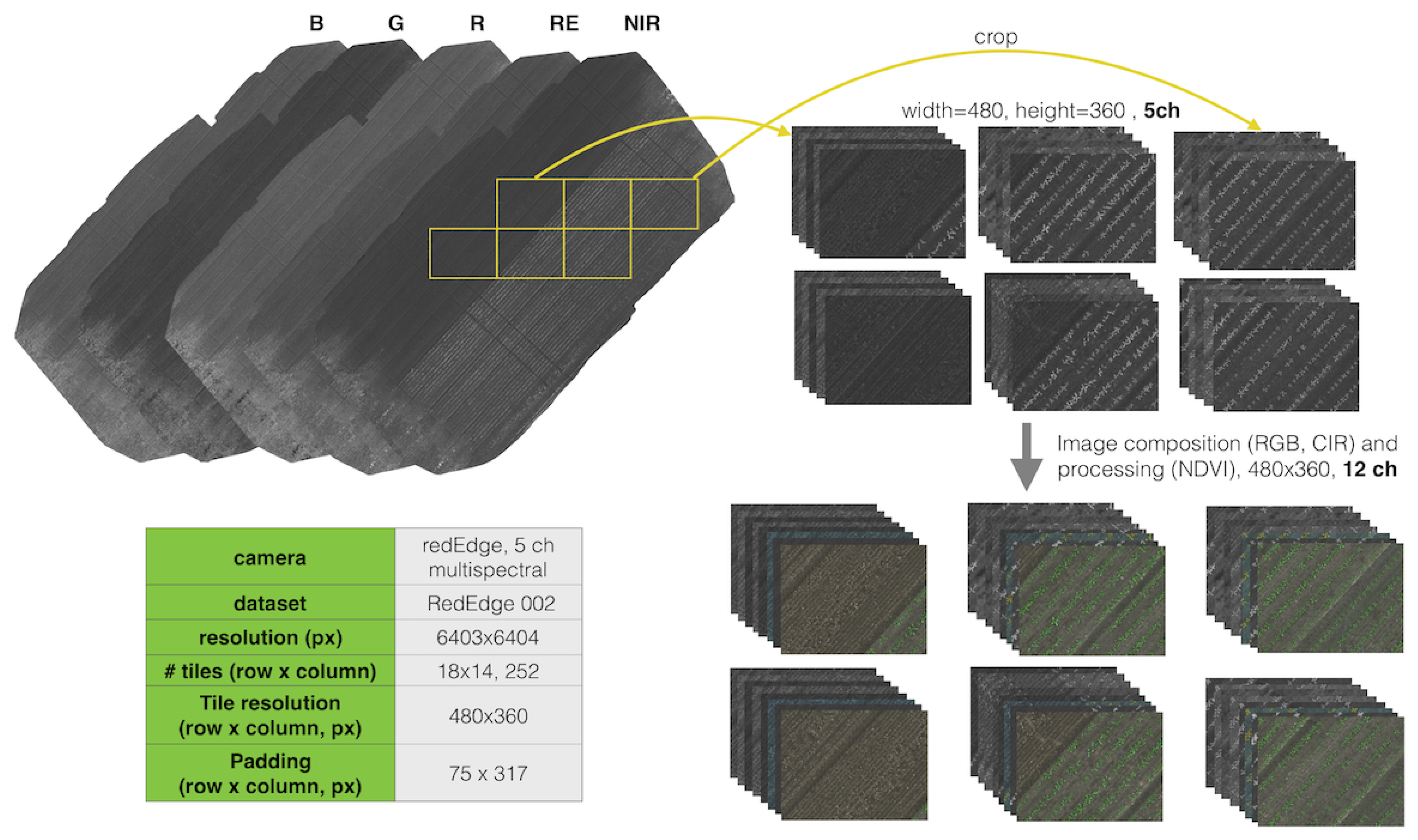
Figure 6.
An illustration of tiling from aligned orthomosaic maps. Multispectral images of fixed size (top right) are cropped from aligned orthomosaic maps (top left). Image composition and preprocessing are then performed for generating RGB, CIR, and NDVI respectively. This yields 12 composited tile channels that are input into a Deep Neural Network (DNN).
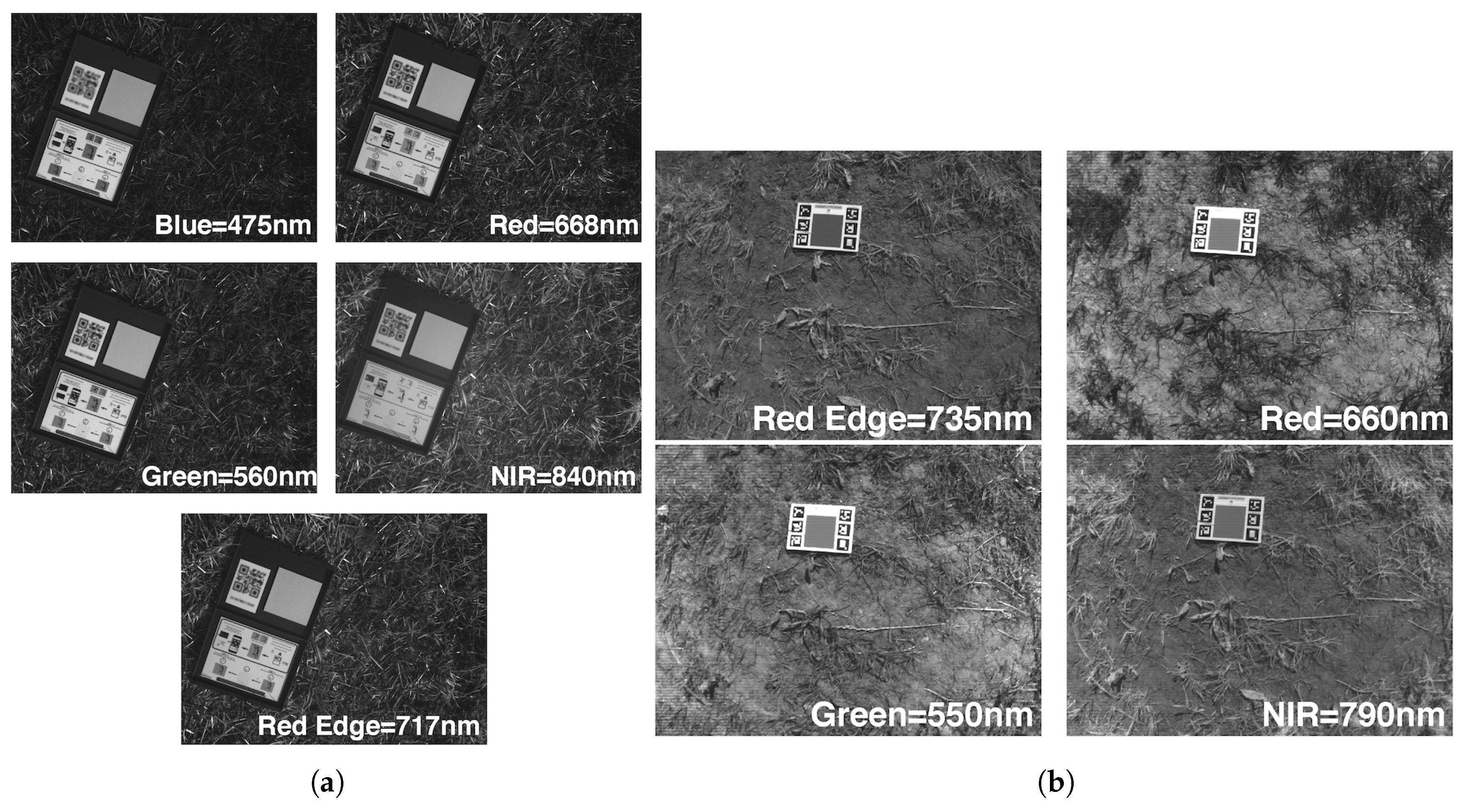
Figure 7.
(a) RedEdge-M radiometric calibration pattern (b) Sequoia calibration pattern for all four bands.
Figure 7.
(a) RedEdge-M radiometric calibration pattern (b) Sequoia calibration pattern for all four bands.
Figure 8.
Our overall processing pipeline. GPS tagged multispectral images are first collected by multiple UAVs and then passed to an orthomosaic tool with images for radiometric calibration. Multi-channel and aligned orthomosaic images are then tiled into a small portion (480 × 360 pixels, as indicated by the orange and green boxes) for subsequent segmentation with a DNN. This operation is repeated in a sliding window manner until the entire orthomosaic map is covered.
Figure 9.
Quantitative evaluation of the segmentation using area under the curve (AUC) of the RedEdge-M dataset. The red box indicates the best model, the black one is our baseline model with only RGB image input, and the blue box is a model with only one NDVI image input.
Figure 9.
Quantitative evaluation of the segmentation using area under the curve (AUC) of the RedEdge-M dataset. The red box indicates the best model, the black one is our baseline model with only RGB image input, and the blue box is a model with only one NDVI image input.
Figure 10.
Performance curves of the RedEdge-M dataset models (Model 1–13). For improved visualization, note that we intentionally omit Model 11, which performs very similarly to Model 10. (a) Model 1; (b) Model 2; (c) Model 3; (d) Model 4; (e) Model 5; (f) Model 6; (g) Model 7; (h) Model 8; (i) Model 9; (j) Model 10; (k) Model 12; (l) Model 13.
Figure 11.
Quantitative evaluation of the segmentation using area under the curve (AUC) of the Sequoia dataset. As in the RedEdge-M dataset, the red box indicates the best model, and the blue box is a model with only one NDVI image input.
Figure 11.
Quantitative evaluation of the segmentation using area under the curve (AUC) of the Sequoia dataset. As in the RedEdge-M dataset, the red box indicates the best model, and the blue box is a model with only one NDVI image input.
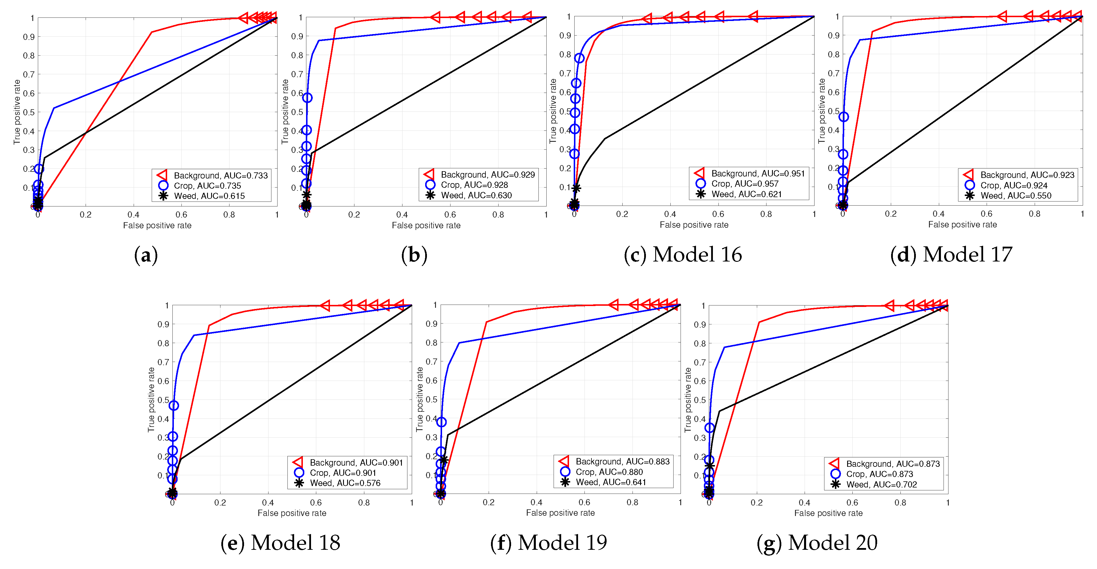
Figure 12.
Performance curves of Sequoia dataset models (Models 14–20). (a) Model 14; (b) Model 15; (c) Model 16; (d) Model 17; (e) Model 18; (f) Model 19; (g) Model 20.
Figure 12.
Performance curves of Sequoia dataset models (Models 14–20). (a) Model 14; (b) Model 15; (c) Model 16; (d) Model 17; (e) Model 18; (f) Model 19; (g) Model 20.
Figure 13.
Quantitative results for the RedEdge-M testing dataset (dataset 003). Each column corresponds to an example input image, ground truth, and the output prediction. Each row (a–f) shows a different zoom level on the orthomosaic weed map. The color convention follows bg, crop, weed. These images are best viewed in color.
Figure 14.
Quantitative results for the Sequoia testing dataset (dataset 005). Each column corresponds to an example input image, ground truth, and the output prediction. Each row (a–f) shows a different zoom level on the orthomosaic weed map. The color convention follows bg, crop, weed. These images are best viewed in color.
Table 1.
Detail of training and testing dataset.
Table 1.
Detail of training and testing dataset.
| Camera | RedEdge-M | Sequoia |
|---|
| Dataset name | 000 | 001 | 002 | 003 | 004 | 005 | 006 | 007 |
Resolution
(col/row)
(width/height) | 5995 × 5854 | 4867 × 5574 | 6403 × 6405 | 5470 × 5995 | 4319 × 4506 | 7221 × 5909 | 5601 × 5027 | 6074 × 6889 |
| Area covered (ha) | 0.312 | 0.1108 | 0.2096 | 0.1303 | 0.1307 | 0.2519 | 0.3316 | 0.1785 |
| GSD (cm) | 1.04 | 0.94 | 0.96 | 0.99 | 1.07 | 0.85 | 1.18 | 0.83 |
Tile resolution
(row/col) pixels | 360/480 |
| # effective tiles | 107 | 90 | 145 | 94 | 61 | 210 | 135 | 92 |
# tiles in row/
# tiles in col | 17×13 | 16×11 | 18 × 14 | 17 × 12 | 13 × 9 | 17 × 16 | 14× 12 | 20 × 13 |
Padding info
(row/col) pixels | 266/245 | 186/413 | 75/317 | 125/290 | 174/1 | 211/459 | 13/159 | 311/166 |
| Attribute | train | train | train | test | train | test | train | train |
| # channels | 5 | 4 |
| Crop | Sugar beet |
Table 2.
Data collection campaigns summary.
Table 2.
Data collection campaigns summary.
| Description | 1st Campaign | 2nd Campaign |
|---|
| Location | Eschikon, Switzerland | Rheinbach, Germany |
| Date, Time | 5–18 May 2017, around 12:00 p.m. | 18 September 2017, 9:18–40 a.m. |
| Aerial platform | Mavic pro | Inspire 2 |
| Camera | Sequoia | RedEdge-M |
| # Orthomosaic map | 3 | 5 |
Training/Testing
multispectral images | 227/210 | 403/94 |
| Crop | Sugar beet |
| Altitude | 10m |
| Cruise speed | 4.8m/s |
Table 3.
Multispectral camera sensors specifications used in this paper.
Table 3.
Multispectral camera sensors specifications used in this paper.
| Description | RedEdge-M | Sequoia | Unit |
|---|
| Pixel size | 3.75 | um |
| Focal length | 5.5 | 3.98 | mm |
| Resolution (width × height) | 1280 × 960 | pixel |
| Raw image data bits | 12 | 10 | bit |
| Ground Sample Distance (GSD) | 8.2 | 13 | cm/pixel (at 120 m altitude) |
| Imager size (width × height) | 4.8 × 3.6 | mm |
| Field of View (Horizontal, Vertical) | 47.2, 35.4 | 61.9, 48.5 | degree |
| Number of spectral bands | 5 | 4 | N/A |
| Blue (Center wavelength, bandwidth) | 475, 20 | N/A | nm |
| Green | 560, 20 | 550, 40 | nm |
| Red | 668, 10 | 660, 40 | nm |
| Red Edge | 717, 10 | 735, 10 | nm |
| Near Infrared | 840, 40 | 790, 40 | nm |
Table 4.
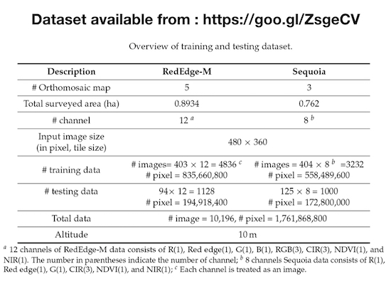
Overview of training and testing dataset.
Table 4.
Overview of training and testing dataset.
| Description | RedEdge-M | Sequoia |
|---|
| # Orthomosaic map | 5 | 3 |
| Total surveyed area (ha) | 0.8934 | 0.762 |
| # channel | 12 | 8 |
Input image size
(in pixel, tile size) | 480 × 360 |
| # training data | # images= 403 × 12 = 4836 | # images = 404 × 8 = 3232 |
| # pixel = 835,660,800 | # pixel = 558,489,600 |
| # testing data | 94× 12 = 1128 | 125 × 8 = 1000 |
| # pixel = 194,918,400 | # pixel = 172,800,000 |
| Total data | # image = 10,196, # pixel = 1,761,868,800 |
| Altitude | 10m |
Table 5.
Performance evaluation summary for the two cameras with varying input channels.
Table 5.
Performance evaluation summary for the two cameras with varying input channels.
| RedEdge-M | AUC |
|---|
| # Model | # Channels | Used Channel | # batches | Cls bal. | Bg | Crop | Weed |
| 1 | 12 | B, CIR, G, NDVI, NIR, R, RE, RGB | 6 | Yes | 0.816 | 0.856 | 0.744 |
| 2 | 12 | B, CIR, G, NDVI, NIR, R, RE, RGB | 4 | Yes | 0.798 | 0.814 | 0.717 |
| 3 | 12 | B, CIR, G, NDVI, NIR, R, RE, RGB | 6 | No | 0.814 | 0.849 | 0.742 |
| 4 | 11 | B, CIR, G, NIR, R, RE, RGB
(NDVI drop) | 6 | Yes | 0.575 | 0.618 | 0.545 |
| 5 | 9 | B, CIR, G, NDVI, NIR, R, RE
(RGB drop) | 5 | Yes | 0.839 | 0.863 | 0.782 |
| 6 | 9 | B, G, NDVI, NIR, R, RE, RGB
(CIR drop) | 5 | Yes | 0.808 | 0.851 | 0.734 |
| 7 | 8 | B, G, NIR, R, RE, RGB
(CIR and NDVI drop) | 5 | Yes | 0.578 | 0.677 | 0.482 |
| 8 | 6 | G, NIR, R, RGB | 5 | Yes | 0.603 | 0.672 | 0.576 |
| 9 | 4 | NIR, RGB | 5 | Yes | 0.607 | 0.680 | 0.594 |
| 10 | 3 | RGB
(SegNet baseline) | 5 | Yes | 0.607 | 0.681 | 0.576 |
| 11 | 3 | B, G, R
(Splitted channel) | 5 | Yes | 0.602 | 0.684 | 0.602 |
| 12 | 1 | NDVI | 5 | Yes | 0.820 | 0.858 | 0.757 |
| 13 | 1 | NIR | 5 | Yes | 0.566 | 0.508 | 0.512 |
| Sequoia | AUC |
| 14 | 8 | CIR, G, NDVI, NIR, R, RE | 6 | Yes | 0.733 | 0.735 | 0.615 |
| 15 | 8 | CIR, G, NDVI, NIR, R, RE | 6 | No | 0.929 | 0.928 | 0.630 |
| 16 | 5 | G, NDVI, NIR, R, RE | 5 | Yes | 0.951 | 0.957 | 0.621 |
| 17 | 5 | G, NDVI, NIR, R, RE | 6 | Yes | 0.923 | 0.924 | 0.550 |
| 18 | 3 | G, NIR, R | 5 | No | 0.901 | 0.901 | 0.576 |
| 19 | 3 | CIR | 5 | No | 0.883 | 0.88 | 0.641 |
| 20 | 1 | NDVI | 5 | Yes | 0.873 | 0.873 | 0.702 |
© 2018 by the authors. Licensee MDPI, Basel, Switzerland. This article is an open access article distributed under the terms and conditions of the Creative Commons Attribution (CC BY) license (http://creativecommons.org/licenses/by/4.0/).

 ,
, 


