How Do Institutional Quality, Natural Resources, Renewable Energy, and Financial Development Reduce Ecological Footprint without Hindering Economic Growth Trajectory? Evidence from China

Abstract

Institutional quality, financial development, and natural resources primarily determine how economic representatives support their operational and production behaviors towards escalating the renewable energy share in the whole energy mix and protecting ecological quality. In this way, this paper is the first to investigate the influence of institutional quality, natural resources, financial development, and renewable energy on economic growth and the environment simultaneously in China from 1996 to 2020. The cointegration approaches verify the presence of a long-run association between the selected variables. The autoregressive distributed lag model outcomes reveal that institutional quality and renewable energy utilization greatly diminish ecological footprint. At the same time, other prospective indicators such as financial expansion and natural resources significantly enhance ecological footprint levels in the short- and long-run. Furthermore, institutional quality, financial expansion, renewable energy, and natural resources significantly trigger economic growth. Besides this, this study has revealed the unidirectional causal association from institutional quality and financial expansion to ecological footprint. In contrast, bidirectional causality occurs between renewable energy, natural resources, ecological footprint, and economic growth. The current research results offer some policy implications that will help to reduce the detrimental influence of environmental deprivation, without hindering the economic growth trajectory in the case of China.

1. Introduction

In the current era, one of the primary objectives in a global society is to diminish the amount of environmental pollution, especially concerning carbon emissions threatening human health. On the other hand, the economic expansion goal is also key for all emerging and high-income nations seeking to increase the living standards of their people. Since 1990, intermediary/transitional economies, such as China, have made significant transformations in their social and economic structures, and achieved elevated growth rates. During this procedure, China’s economy has increased the deployment of energy-intensive resources, such as fossil fuels (e.g., oil, gas, and coal). Their contribution to global environmental pollution increased manifold. Owing to significant greenhouse gas emissions, the sustainable development goal does not seem pragmatic in the short term.

In 1949, the Chinese Communist Party came into power, and initiated reforms in the late 1980s. China has become the world’s fastest-growing country, with a constant growth rate of approximately 9%. Trade openness is approximately 38% of the GDP in China, it being the biggest exporter and second-leading importer of goods in the world, which is remarkable [1]. In the early 1950s, economists found that countries that were rich in resources grew slower compared to those deprived, which is a question of concern. Resources are the base of development. Those nations that are abundant in natural resources are more capable of converting resources into development, so more production leads to more exports. Countries that enjoy a wealth of natural resources tend to have more incentives to avoid economic diversification (Dunning, 2005).

It can be observed that strong institutions lead to a strong nation and a base of economic development for that country. Differences in regional growth are basically due to institutional differences. The natural resource growth in a country creates two types of effects; one is the output effect, and the other is an institutional effect [2,3]. The Heckscher–Ohlin theory and bulk product theory support the argument that a country abundant in natural resources can promote growth better than those with less abundant resources [4]. In contrast, this is not seen as valid in all cases. The countries endowed with natural resources are less economically developed compared to developed economies that are less abundant in natural resources. In China, natural resources are not evenly distributed between provinces and coastal areas such as Jiangsu, which has educated its people to develop more natural and human resources to improve industrial productivity. Theories have been devised regarding this question, primarily the Dutch disease model [5] and institutional quality.

Several studies have investigated the significance of institutional excellence, as a result of which abundant resources may increase economic growth and thus lead to corruption and rent-seeking actions [6,7,8,9]. In this regard, Ross [10] argued that institutions can endogenously encourage economic growth via resource endowments. However, the existing literature claims that institutional excellence can explain many cross-country differences in economic expansion [11]. The quality of institutions varies between provinces in a country. In China, provinces have homogeneous legal and constitutional systems, while institutional superiority differs from a historical perspective.

Furthermore, conventional and new economic theories have extensively addressed economic development. Current studies on institutional economics have attempted to provide a framework for institutional quality and the measurement of this qualitative subject [12]. A high-quality institutional framework increases the growth pace by incentivizing economic activities, for instance, improving efficiency and resource allocation more competently. Protecting property rights and reducing transaction costs and rent-seeking behavior supports freedom of choice, and eases economic growth scenarios [13].

Environmental deprivation occurs owing to the unnecessary deployment of natural resources to prepare and extract diverse raw substances/materials that directly affect the atmosphere, such as via water shortfalls, soil erosion, halting biodiversity, worldwide warming aggravation, and the destruction of environmental capacities. The consumption of such raw substances has become the primary source of greenhouse gas (GHG) emissions in the atmosphere. In contrast, the deployment of natural resources has a twofold impact on GDP growth: the prompt use of natural resources boosts the production level and intensifies the diminution rate. The consumption of natural resources has particular effects on diverse investors that stipulate GDP growth. Conversely, the excessive use of (overexploited) natural resources also increases the exhaustion rate and rapidly reduces resources. Over-dependence on the consumption of natural resources is not a helpful approach for achieving a sustainable environment and economic development [14].

The studies also found an indirect effect of institutional value on economic growth through trade openness. Institutional quality has strengthened economic growth, giving rise to trade as the best institutional value. Conversely, developing economies have fewer trade advantages, raising concerns about the reduction in institutional value. Institutional quality escalates economic growth and facilitates technology and knowledge transfer among the countries. It is essential and time-consuming to discover the association within the natural resource, growth, energy, institutional quality, and environmental nexus. Institutions are different from one another. They have their mechanisms and policy statements. Finally, the authors conclude that institutions have specific characteristics, so comprehensive analysis is required based on theoretical and empirical analysis to derive robust results regarding their impact on growth and the environment in the presence of energy and natural resources. The main novelty of this paper is that, from an analytical and theoretical perspective, the institutional factors, along with financial development, energy use, and natural resources, are assessed in relation to economic growth and the environment simultaneously, which is under-investigated in the existing literature. Secondly, renewable energy is used in exploring this nexus, because China is paying more attention to this factor, and trying to achieve growth along with a stable environment. The novelty of this study is that it provides new arguments regarding the influence on economic growth of renewable energy, financial expansion, institutional quality, and natural resources in both the short- and long-run. In the most recent literature, institutional economics has emerged in determining economic growth and the environment, and recent studies have tried to determine the impact of institutional quality on the environment. The outlook of this research is an effort to explore this nexus in the case of the Chinese economy.

Moreover, economic growth theories, models, and their quantitative impact via human capital, physical capital, labor, and technology have been analyzed. However, in recent times, it has been observed that institutional quality, financial expansion, and natural resources have a strong effect on the environment and economic growth. Hence, this study tries to investigate how institutional quality, natural resources, alternative and renewable energy use, and financial progress trigger economic activities and protect ecological excellence in the case of China.

The remaining sections of the present research are reported as follows: Section 2 contains a literature review. The data, economic modeling, and methods are explored in Section 3. Empirical findings and the discussion are given in Section 4, and further, this section outlines the robustness checks. Finally, the conclusion and policy suggestions are provided in Section 5 accordingly.

2. Review of Literature

The attempt to reduce ecological footprints and protect the environment is essential today. Studies that analyze the relationship between economic growth and variables such as human capital, physical capital, and natural resources are becoming increasingly essential. The works in the literature show the different statistical methods used, highlighting the wide variety of possible methods, such as Panel ARDL or the Generalized Method of Moments.

Several studies argue that energy affects country growth [15,16,17]. Ji et al. [18] analyzed the interaction among natural resource abundance, GDP growth, and institutional excellence. They found that natural resources have a constructive influence on economic growth in the case of China. Similarly, Asghar et al. [19] attempted to elucidate the influence of institutional value on GDP growth in emerging Asian nations using panel ARDL. This study found that institutional eminence significantly enhances GDP growth. Moreover, Nguyen et al. [20] observed the effects of institutional worth on GDP growth for 29 developing countries from 2002 to 2015 through sys-GMM (Generalized Method of Moments) estimators. The empirical outcomes revel that institutional quality boosts economic growth.

Conversely, Poshakwale and Ganguly [21] analyzed the transmission channels of international shocks on the GDP growth of developing markets, and found that the mean impact of international shocks on developing markets’ growth is insignificant. However, there is variation both over time and across sections. Taken as a whole, there is an important effect on GDP growth. Chan et al. [22] examined the moderating role of institutional structure on the impact of market attentiveness in ASEAN-5 countries (Indonesia, Malaysia, the Philippines, Singapore, and Thailand). They observed that higher bank attentiveness diminishes the competence level in the case of commercial banks. They used the Slack-Based Measures Data Envelopment Analysis and the Generalized Method of Moments system.

On the other hand, an improved institutional structure considerably advances bank competence, which results in higher industry concentration. An institutional system can affect a firm’s choices. In contrast, in countries with low legal institutional quality and economic development, imports of technological equipment have an insignificant impact on provincial innovation potential [23]. Similarly, in developing countries, Peres et al. [24] showed that the impact of institutional excellence is not significant because of the weak institutional structure, and governance indicators tend to be key in attracting the inflow of foreign investment. The role of institutions at the provincial level is also analyzed in the literature. For example, using panel data, Qiang and Jian [25] employed provincial longitudinal data from 2005 to 2018, and categorized institutional indicators by the degree of market openness, market resource allocation, and property rights diversification. The authors show that the “resource curse” proposition is appropriate for provincial-level data in China.

Furthermore, it was found that increasing market openness could ease the resource curse in all studies, with mixed results. In this context, Tsani [26] studied the association between governance, institutional excellence, resource funds, and their role in tackling the resource curse. They harmonized the debate on the resource curse and institutional quality and governance determinants. They found that resource funds are important when addressing the worsening of governance and institutional quality as a result of resource wealth. Similarly, Shuai and Zhongying [27], based on the resource curse hypothesis, revealed a negative relationship between real income growth and energy utilization. However, a sector-wise study of institutional excellence and income growth in African and Asian countries found contrary results.

In the context of financial expansion, Jalil and Feridun [28], using the autoregressive distributed lag (ARDL), inspected the role of financial improvement in influencing environmental deprivation in the case of China. The outcomes show that financial development has led to reduced environmental degradation. However, the environmental Kuznets curve (EKC) relationship is valid in the case of China. The EKC hypothesis holds that the relationship between environmental degradation and per capita income follows an inverted U-shaped path. Similarly, Al-Mulali et al. [29] found that financial growth promotes atmospheric quality worldwide. Adebanjo and Shakiru [30] found that the EKC shows that economic growth has positively and negatively impacted Jordanian air pollution. In contrast, Boutabba [31] reported that a robust financial sector significantly increases CO₂ emissions.

Additionally, the Granger causality test reports that unidirectional causality pertains from financial expansion to energy utilization and CO₂ emissions in the case of the Indian economy. In a massive study by Omri et al. [32], found a similar bidirectional causality between CO₂ emissions and real income was observed. This study also considered the long-term link between real income, financial expansion, and carbon emissions for MENA countries. The findings of the simultaneous equation model reveal that bidirectional causality exists between CO₂ emissions and real income growth. In this regard, Zaidi et al. [33] indicated that the financial progress of an economy encompasses purchasers, and attains reliability and durability in commodities, which enhances the overall energy demand and environmental damages.

Early studies, such as that of Hartwick [34], argued that natural resource wealth positively affects the production of renewable energies, as it would increase the capital available for investment. There are also works focusing on some specific areas, such as that of Baloch et al. [35] for BRICS, which shows that natural resources are not environmentally friendly in the case of South Africa due to the unsustainable consumption of natural resources. Adebanjo and Adeoye [36] concluded that natural resources significantly negatively influence economic growth in 10 sub-Saharan African countries. The abundance of natural resources tends to favor renewable energy production in a country. Still, certain natural resources, such as oil, can be detrimental due to their potentially corrosive effect on the economy and governance [37]. Dagar et al. [38] demonstrated that renewable energy consumption and natural resources contribute to reducing environmental degradation. In addition, they assert that financial development, GDP growth, and natural resources promote expansion in cleaner energy diligence, and enable governments and policy makers to reduce pollution levels.

Epo and Faha [39] probed the functions of institutional quality, natural resources, and income growth in 44 African economies from 1996 to 2016. They a conducted cross-sectional instrumental variables analysis, dynamic panel data instrumental variables regression, and panel smooth transition regression. The connection between real income growth and natural resources varies with natural resources and institutional quality measures. Egbetokun et al. [40] concluded in the case of Nigeria that institutional value protects environmental quality in the context of the economic growth trajectory. Furthermore, Khan et al. [41] studied the financial development and natural resource nexus by assessing the critical role of institutional superiority using ARDL dynamic simulations. The results reveal that natural resource have an adverse impact on financial expansion.

Furthermore, institutional excellence has a moderate impact on resource finance, while the threshold level of the impact is ambiguous sometimes; it is sometimes positive and sometimes negative. Conversely, the impact of institutional quality and financial expansion on the environment was investigated by Godil et al. [42], who found that institutional quality has a constructive impact on carbon emissions in the long-run. Moreover, the ICT sector and financial development have adverse impacts on carbon emissions. Similarly, Elsalih et al. [43] inspected the association between environmental performance and institutional value in 28 oil-producing economies from 2002 to 2014, revealing that institutional excellence plays a vital role in enhancing ecological performance, and supporting the theoretical background of the EKC hypothesis. In addition, Yousaf et al. [44] studied the impact of the ecological footprint of energy and fossil consumption in the case of Pakistan using ARDL and fully modified ordinary least squares (FMOLS). They found that fossil fuel is a leading factor in environmental degradation. Population growth and fossil fuel negatively impact the environment. In the same context, in the case of China, the ecological footprint increases growth driven by fossil fuels. The study explored this issue within the literature, but hardly found any studies examining the associations between institutional quality, financial expansion, natural resources along with renewable energy, and ecological footprints to investigate the impact of environmental degradation and income growth simultaneously in China. Therefore, this research is an attempt to expand the literature on the subject in the Chinese context.

3. Data, Model, and Methodology

3.1. Data and Functions Description

The major objective of this paper is to discover the influence of institutional quality, financial expansion, natural resources, and renewable energy on ecological footprint and economic growth from 1996 to 2020 in China. Regarding the description of the variables, institutional quality (INSQ) represents a broad concept that encompasses law, individual rights, regulation, and high-quality government services. This paper measures institutional quality based on the international country risk guide (ICRG) index. This index is based on 22 variables encompassing three risk groups: political, financial, and economical. This index is calculated for each of these groups (the political risk index is based on 100 points, the financial risk index on 50 points, and the economic risk index on 50 points), from which the ICRG index is obtained. The index scores range from 0 to 100, with low risk from 80 to 100 points and very high risk from 0 to 49.9 points.

Financial expansion is the capacity to strengthen the financing of a country, region, or company. The authors define financial development as financial credit offered by the financial sector as the % of GDP [45]. Furthermore, natural resources are raw materials found in nature that can be used for production or consumption. We measure natural resources, NR, via natural resource rent which is a ratio of all natural resource rents to GDP calculated as Constant 2010 USD. It comprises coal, oil, mineral, gas, and forest rents. The authors applied this proxy for a couple of reasons. Firstly, this is the most suitable proxy for resource revenue because it measures resource revenues that are extra effective for rent-seeking, etc. Secondly, this proxy has been extensively used in recent literature [46].

For the comprehensive analysis, we have used two models; one is used to discover the impact of the variables mentioned above on growth, and the second model is used to find the effect of such time series on the environment.

Table 1. Variables’ description and data source.

Acronyms	Variables	Description	Variables Justification
GDP	Gross domestic product	Constant 2010 USD	[19,30,32,45,47]
INSQ	Institutional quality	ICRG index	[9,23,46,48,49]
FD	Financial development	Domestic credit to the private sector (% of GDP)	[29,50,51,52]
NR	Natural resource rents	% of GDP	[25,53,54,55,56]
REN	Renewable energy use	Share of all final energy use

explores the study variables’ description and the data source.

$$\mathbf{Model}\mathbf{1}\mathbf{:}\mathrm{EFP}=\mathrm{f}\left(\mathrm{INSQ},\mathrm{FD},\mathrm{NR},\mathrm{REN}\right)$$

(1)

$$\mathbf{Model}\mathbf{2}\mathbf{:}\mathrm{GDP}=\mathrm{f}\left(\mathrm{INSQ},\mathrm{FD},\mathrm{NR},\mathrm{REN}\right)$$

(2)

Equations (1) and (2) explain the functional relation of dependent and independent variables. To address the issues of heteroscedasticity, scale equivalence, data sharpness, and autocorrelation, this study transformed the model into a logarithmic form.

$$\mathrm{Ln}({\mathrm{EFP}}_{\mathrm{t}})={\mathsf{\alpha }}_0+{\mathsf{\alpha }}_1\mathrm{Ln}({\mathrm{INSQ}}_{\mathrm{t}})+{\mathsf{\alpha }}_2\mathrm{Ln}({\mathrm{FD}}_{\mathrm{t}})+{\mathsf{\alpha }}_3\mathrm{Ln}({\mathrm{NR}}_{\mathrm{t}})+{\mathsf{\alpha }}_4\mathrm{Ln}({\mathrm{REN}}_{\mathrm{t}})+{\mathsf{\epsilon }}_{\mathrm{t}}$$

(3)

$$\mathrm{Ln}({\mathrm{GDP}}_{\mathrm{t}})={\mathsf{\beta }}_0+{\mathsf{\beta }}_1\mathrm{Ln}({\mathrm{INSQ}}_{\mathrm{t}})+{\mathsf{\beta }}_2\mathrm{Ln}({\mathrm{FD}}_{\mathrm{t}})+{\mathsf{\beta }}_3\mathrm{Ln}({\mathrm{NR}}_{\mathrm{t}})+{\mathsf{\beta }}_4\mathrm{Ln}({\mathrm{REN}}_{\mathrm{t}})+{\mathsf{\epsilon }}_{\mathrm{t}}$$

(4)

Equations (3) and (4) explain the econometric model of the concerned variables, where Ln denotes the natural logarithm algorithm, EFP denotes ecological footprint, INSQ is institutional quality, FD represents financial development, NR illustrates natural resources, and REN shows renewable energy. The subscript t of every variable shows the time dimension of the respective variable. Moreover, ${\mathsf{\alpha }}_0{\mathrm{and}\mathsf{\beta }}_0$ represent the intercept terms of their respective functions. The terms ${\mathsf{\alpha }}_1\to {\mathsf{\alpha }}_4{\mathrm{and}\mathsf{\beta }}_1\to {\mathsf{\beta }}_4$ indicate the regressors’ elasticity and ${\epsilon }_t$ indicates the stochastic error term.

3.2. Empirical Methodology

A comprehensive econometric process involves the three steps of (i) time series unit root analysis, (ii) cointegration analysis, and (iii) long-run and short-run elasticity estimation.

3.2.1. Time Series Unit Root Test

The stationary analysis is the first phase in the time series data analysis because the outcomes from regression analysis provide misleading/inconsistent information if the candidate regressors show a stochastic trend [57]. The empirical regression outcomes are misleading and spurious if this stochastic trend is detected in a minimum of one regressor and a dependent variable, or if both of these time series have no cointegration [58]. To evade this issue, the Phillips–Perron (PP) [59] and Augmented Dickey–Fuller (ADF) [60] stationarity tests were performed on the candidate time variables. Both ADF and PP unit root tests have a lower ability to determine the integration order of the selected variables due to the small sample size (<20) for China. In this regard, we have applied the Kwiatkowski–Phillips–Schmidt–Shin (KPSS) test developed by Kwiatkowski et al. [61] to examine the integration order and stationarity of the selected time series variables for a small sample size. The mathematical approach of ADF and PP stationarity tests can be explored in the first-order autoregressive (AR) model, the autoregressive model with consistency but no trend, and the autoregressive model with consistency and trend.

The first-order AR model:

$${\mathsf{\Delta }\mathrm{X}}_{\mathrm{t}}={\mathsf{\Psi }\mathsf{\Delta }\mathrm{X}}_{\mathrm{t}-1}+{\displaystyle \sum }_{\mathrm{j}=2}^{\mathrm{q}}{\mathsf{\delta }}_{\mathrm{j}}{\mathsf{\Delta }\mathrm{X}}_{\mathrm{t}-\mathrm{j}+1}+{\mathsf{\mu }}_1$$

(5)

The AR model with only consistency:

$${\mathsf{\Delta }\mathrm{X}}_{\mathrm{t}}={\mathsf{\Psi }\mathsf{\Delta }\mathrm{X}}_{\mathrm{t}-1}+\mathrm{c}+{\displaystyle \sum }_{\mathrm{j}=2}^{\mathrm{q}}{\mathsf{\delta }}_{\mathrm{j}}{\mathsf{\Delta }\mathrm{X}}_{\mathrm{t}-\mathrm{j}+1}+{\mathsf{\mu }}_1$$

(6)

The AR model with both consistency and trend:

$${\mathsf{\Delta }\mathrm{X}}_{\mathrm{t}}={\mathsf{\Psi }\mathsf{\Delta }\mathrm{X}}_{\mathrm{t}-1}+\mathrm{c}+\mathrm{bt}+{\displaystyle \sum }_{\mathrm{j}=2}^{\mathrm{q}}{\mathsf{\delta }}_{\mathrm{j}}{\mathsf{\Delta }\mathrm{X}}_{\mathrm{t}-\mathrm{j}+1}+{\mathsf{\mu }}_1(\mathrm{with}~>{\mathsf{\mu }}_{\mathrm{t}}~>BB\left(0,{\mathsf{\sigma }}_{\mathsf{\epsilon }}^2\right)$$

(7)

The models above apply to the null hypothesis (H₀), stating that the study variables contain mean, auto-covariance, and non-constant variance. Considering this, the PP stationary method also employs analogous models; however, it is dissimilar from other approaches because it relies on non-parametric correction for the recognition of serial correlation.

3.2.2. Johansen Cointegration Test

This study explores the long-run association between selected variables in the second step. In this way, the two time series are interpreted to be cointegrated over the long term if they progress simultaneously over time, and the distance between them is constant. Even when all the selected variables are integrated in the same order, the Johansen maximum likelihood test [62] is applied to check the long-run cointegration association between the selected variables. Consequently, the long-run cointegration association reveals the existence of a long-run steady-state equilibrium, towards which the system of economics converges in due course. The differences (or error terms) in the long-run cointegration relationship equation are deduced as the distorted error for a particular point in time.

This study applies the Johansen [63] long-run cointegration approach to test the long-term constancy and steady-state equilibrium between candidate variables via the following mathematical expressions/equation:

$${\mathsf{\Delta }\mathrm{Y}}_{\mathrm{t}}={\mathsf{\lambda }}_{\mathrm{t}-1}+{\displaystyle \sum }_{\mathrm{i}=1}^{\mathrm{q}-1}{\mathsf{\theta }}_{\mathrm{i}}{\mathsf{\Delta }\mathrm{Y}}_{\mathrm{t}-1}+{\mathsf{\delta }\mathrm{x}}_{\mathrm{t}}+{\mathsf{\mu }}_{\mathrm{t}}$$

(8)

$$\mathsf{\lambda }={\displaystyle \sum }_{\mathrm{i}=1}^{\mathrm{q}}{\mathrm{M}}_{\mathrm{i}}-\mathrm{I},{\mathsf{\theta }}_{\mathrm{i}}=-{\displaystyle \sum }_{\mathrm{i}=\mathrm{t}+1}^{\mathrm{q}}{\mathrm{M}}_{\mathrm{j}}$$

(9)

In Equations (8) and (9), the term λ is a parameter matrix of the adjusted disequilibrium. The stacking of coefficient M increased the unobserved factor’s change speed to offset the disequilibrium association. The term θ is applied to confine the dynamic short-run adjustment [63,64].

3.2.3. Autoregressive Distributed Lag (ARDL) Bound and Other Long-Run Estimation Tests

The bounds cointegration test for the long-run association among series, also known as the autoregressive distributed lag (ARDL) method, is extensively employed owing to its numerous benefits. This process addresses many problems, such as the inability to assess the hypotheses on the approximated parameters in the long-run, and endogeneity issues. The ARDL test can check for the presence of long-term connections among the studied time series in levels, even if the underlying explanatory variables are entirely level I(0), purely different I(1), or mutually/mixed cointegrated I(0,1). Moreover, the ARDL test can approximate both the model’s long- and short-run elasticities. In addition, the bound testing method has more advanced small sample properties (micro-numerasticity) than multivariate ones [65,66].

In contrast to the error correction model (ECM) and ordinary least square (OLS) regression, the ARDL test applies imbalanced error correction term parameters to investigate the long-run cointegration/association among the selected time series variables. This uneven use of parameters is useful for the application of the ARDL bounds approach, which can be further applied to establish the long-term relationship [67], as mentioned in Equations (10) and (11):

$${\mathsf{\Delta }\mathrm{Y}}_{\mathrm{t}}={\mathsf{\delta }}_0+\sum {\mathsf{\delta }}_{\mathrm{i}}{\mathsf{\Delta }\mathrm{Y}}_{\mathrm{t}-\mathrm{i}}+\sum {\mathsf{\pi }}_{\mathrm{j}}{\mathsf{\Delta }\mathrm{X}}_{1,\mathrm{t}-\mathrm{j}}+\sum {\mathsf{\beta }}_{\mathrm{k}}{\mathsf{\Delta }\mathrm{X}}_{2,\mathrm{t}-\mathrm{k}}+{\mathsf{\Phi }\mathrm{ECT}}_{\mathrm{t}-1}$$

(10)

$${\mathsf{\Delta }\mathrm{Y}}_{\mathrm{t}}={\mathsf{\delta }}_0+\sum {\mathsf{\delta }}_{\mathrm{i}}{\mathsf{\Delta }\mathrm{Y}}_{\mathrm{t}-\mathrm{i}}+\sum {\mathsf{\pi }}_{\mathrm{j}}{\mathsf{\Delta }\mathrm{X}}_{1,\mathrm{t}-\mathrm{j}}+\sum {\mathsf{\beta }}_{\mathrm{k}}{\mathsf{\Delta }\mathrm{X}}_{2,\mathrm{t}-\mathrm{k}}+{\mathsf{\xi }}_0{\mathrm{Y}}_{\mathrm{t}-1}+{\mathsf{\xi }}_1{\mathrm{X}}_{1,\mathrm{t}-1}+{\mathsf{\xi }}_2{\mathrm{X}}_{2,\mathrm{t}-1}+{\mathsf{\epsilon }}_{\mathrm{t}}$$

(11)

where Equation (12) portrays the unrestricted estimated error correction model just before long-run relationship testing with the ARDL bounds test, as follows:

$$\begin{gathered} {\mathsf{\Delta }\mathrm{CE}}_{\mathrm{t}}=\mathsf{\theta }+{\displaystyle \sum }_{\mathrm{i}=1}^{\mathrm{k}}{\mathsf{\delta }}_0{\mathsf{\Delta }\mathrm{CE}}_{\mathrm{t}-\mathrm{i}}+{\displaystyle \sum }_{\mathrm{i}=1}^{\mathrm{k}}{\mathsf{\delta }}_1{\mathsf{\Delta }\mathrm{X}}_{1,\mathrm{t}-\mathrm{i}}+{\displaystyle \sum }_{\mathrm{i}=1}^{\mathrm{k}}{\mathsf{\delta }}_2{\mathsf{\Delta }\mathrm{X}}_{2,\mathrm{t}-\mathrm{i}}+{\displaystyle \sum }_{\mathrm{i}=1}^{\mathrm{k}}{\mathsf{\delta }}_3{\mathsf{\Delta }\mathrm{X}}_{3,\mathrm{t}-\mathrm{i}}+{\displaystyle \sum }_{\mathrm{i}=1}^{\mathrm{k}}{\mathsf{\delta }}_4{\mathsf{\Delta }\mathrm{X}}_{4,\mathrm{t}-\mathrm{i}}+{\mathsf{\lambda }}_{0}ln{\mathsf{\Delta }\mathrm{CE}}_{\mathrm{t}-\mathrm{i}}+{\mathsf{\lambda }}_{1}ln{\mathrm{X}}_{1,\mathrm{t}-\mathrm{i}} \\ +{\mathsf{\lambda }}_2{\mathrm{lnX}}_{2,\mathrm{t}-\mathrm{i}}+{\mathsf{\lambda }}_3{\mathrm{lnX}}_{3,\mathrm{t}-\mathrm{i}}+{\mathsf{\lambda }}_4{\mathrm{lnX}}_{4,\mathrm{t}-\mathrm{i}}+{\mathsf{\delta }}_5\mathrm{T}+{\mathsf{\delta }}_6\mathrm{B}+{\mathsf{\mu }}_{\mathrm{t}} \end{gathered}$$

(12)

where i denotes the cross-section, t presents the time span, and Δ shows the first difference operator. The null hypothesis concerning the absence of a long-term connection between the time series indicators can be reported in Equation (13) as:

$${\mathsf{\lambda }}_0={\mathsf{\lambda }}_1={\mathsf{\lambda }}_2={\mathsf{\lambda }}_3={\mathsf{\lambda }}_4=0$$

(13)

$$\begin{gathered} {\mathsf{\Delta }\mathrm{lnCE}}_{\mathrm{t}}=\mathsf{\theta }+{\displaystyle \sum }_{\mathrm{i}=1}^{\mathrm{k}}{\mathsf{\delta }}_0{\mathsf{\Delta }\mathrm{lnCE}}_{\mathrm{t}-\mathrm{i}}+{\displaystyle \sum }_{\mathrm{i}=1}^{\mathrm{k}}{\mathsf{\delta }}_1{\mathsf{\Delta }\mathrm{X}}_{1,\mathrm{t}-\mathrm{i}}+{\displaystyle \sum }_{\mathrm{i}=1}^{\mathrm{k}}{\mathsf{\delta }}_2{\mathsf{\Delta }\mathrm{X}}_{2,\mathrm{t}-\mathrm{i}}+{\displaystyle \sum }_{\mathrm{i}=1}^{\mathrm{k}}{\mathsf{\delta }}_3{\mathsf{\Delta }\mathrm{X}}_{3,\mathrm{t}-\mathrm{i}} \\ +{\displaystyle \sum }_{\mathrm{i}=1}^{\mathrm{k}}{\mathsf{\delta }}_4{\mathsf{\Delta }\mathrm{X}}_{4,\mathrm{t}-\mathrm{i}}+{\mathsf{\delta }}_5\mathrm{T}+{\mathsf{\delta }}_6\mathrm{B}+{\mathsf{\delta }}_7{\mathrm{ECT}}_{\mathrm{t}-1}+{\mathrm{w}}_{\mathrm{t}} \end{gathered}$$

(14)

The ARDL bounds method employs non-standard asymptotic distribution and the joint F-statistic with the H₀ of the nonexistence of a long-run connection based on Equations (15) and (16). This process entails calculating two sets of critical values, the upper critical and the lower critical bound. The null hypothesis will be discarded if the approximated joint F-statistic value is higher than the upper bound. The null hypothesis will be accepted when the approximated joint F-statistic value is less than the lower bound limit.

3.2.4. Short-Run Elasticity Estimates

After variable transformation, the short-term elasticity of the variables mentioned above was approximated using the ARDL-based error correction model as:

$${\mathrm{lnY}}_{\mathrm{t}}={\mathsf{\Psi }}_0+{\displaystyle \sum }_{\mathrm{i}=1}^{\mathrm{q}}{\mathsf{\Psi }}_{1\mathrm{i}}{\mathrm{lnY}}_{\mathrm{t}-\mathrm{i}}+{\displaystyle \sum }_{\mathrm{i}=0}^{\mathrm{q}}{\mathsf{\Psi }}_{2\mathrm{i}}{\mathrm{lnX}}_{1,\mathrm{t}-\mathrm{i}}+{\displaystyle \sum }_{\mathrm{i}=0}^{\mathrm{q}}{\mathsf{\Psi }}_{3\mathrm{i}}{\mathrm{lnX}}_{2,\mathrm{t}-\mathrm{i}}+{\displaystyle \sum }_{\mathrm{i}=0}^{\mathrm{q}}{\mathsf{\Psi }}_{4\mathrm{i}}{\mathrm{lnX}}_{3,\mathrm{t}-\mathrm{i}}+{\displaystyle \sum }_{\mathrm{i}=0}^{\mathrm{q}}{\mathsf{\Psi }}_{5\mathrm{i}}{\mathrm{X}}_{4,\mathrm{t}-\mathrm{i}}+{\mathsf{\lambda }\mathrm{ECM}}_{\mathrm{t}-1}+{\mathsf{\epsilon }}_{\mathrm{t}}$$

(15)

In Equation (15), ECM_t-1 shows the error correction term that was acquired by employing the following equation:

$${\mathrm{ECM}}_{\mathrm{t}}={\mathrm{lnY}}_{\mathrm{t}}-{\mathsf{\beta }}_0-{\displaystyle \sum }_{\mathrm{i}=1}^{\mathrm{q}}{\mathsf{\beta }}_{1\mathrm{i}}{\mathrm{lnY}}_{\mathrm{t}-\mathrm{i}}-{\displaystyle \sum }_{\mathrm{i}=0}^{\mathrm{q}}{\mathsf{\delta }}_{2\mathrm{i}}{\mathrm{lnX}}_{1,\mathrm{t}-\mathrm{i}}-{\displaystyle \sum }_{\mathrm{i}=0}^{\mathrm{q}}{\mathsf{\delta }}_{3\mathrm{i}}{\mathrm{lnX}}_{2,\mathrm{t}-\mathrm{i}}-{\displaystyle \sum }_{\mathrm{i}=0}^{\mathrm{q}}{\mathsf{\delta }}_{4\mathrm{i}}{\mathrm{lnX}}_{3,\mathrm{t}-\mathrm{i}}-{\displaystyle \sum }_{\mathrm{i}=0}^{\mathrm{q}}{\mathsf{\delta }}_{5\mathrm{i}}{\mathrm{X}}_{4,\mathrm{t}-\mathrm{i}}$$

(16)

where λ denotes the convergence speed from short- to long-run stable equilibrium, and all coefficients, such as Ψ₁, Ψ₂, Ψ₃, Ψ₄, Ψ₅, and Ψ₆, illustrate the parameters to be estimated.

3.2.5. Granger Causality Test

After detecting the short-run and long-run elasticity of the regressors, it is vital to determine the causal link between the study’s time series. To do this, the Granger causality approach [68] can discover the association (either negative or positive), and whether the assessed variable influences explanatory variables or not. In the Granger causality approach, Granger [68] advocates vector autoregressive model approximations of the causal link between selected time series. In this regard, the present study follows the process of discovering the causal connections between variables as presented in Equations (17) and (18):

$${\mathrm{Y}}_{\mathrm{t}}={\mathsf{\beta }}_0+{\displaystyle \sum }_{\mathrm{i}=1}^{\mathrm{m}}{\mathsf{\beta }}_{\mathrm{i}}{\mathrm{Y}}_{\mathrm{t}-\mathrm{i}}+{\displaystyle \sum }_{\mathrm{i}=1}^{\mathrm{m}}{\mathsf{\eta }}_{\mathrm{i}}{\mathrm{X}}_{\mathrm{t}-\mathrm{i}}+{\mathsf{\mu }}_{\mathrm{t}}$$

(17)

$${\mathrm{X}}_{\mathrm{t}}={\mathsf{\beta }}_0+{\displaystyle \sum }_{\mathrm{j}=1}^{\mathrm{k}}{\mathsf{\alpha }}_{\mathrm{j}}{\mathrm{Y}}_{\mathrm{t}-\mathrm{j}}+{\displaystyle \sum }_{\mathrm{j}=1}^{\mathrm{k}}{\mathsf{\beta }}_{\mathrm{j}}{\mathrm{X}}_{\mathrm{t}-\mathrm{j}}+{\mathsf{\mu }}_{\mathrm{t}}$$

(18)

4. Results and Discussion

4.1. Descriptive Statistics and Correlation Matrix

Table 2. Descriptive statistics.

Stats.	LnEFP	LnGDP	LnINSQ	LnFD	LnNR	LnREN
Mean	1.015826	15.18082	4.227274	4.823501	1.009460	6.396785
Median	1.071201	15.34033	4.197310	4.812964	0.909565	6.498880
Maximum	1.316077	16.50490	4.391596	5.206381	2.272676	7.677059
Minimum	0.605814	13.66904	4.020657	4.493742	0.046189	5.244948
Std. Dev.	0.283064	1.008818	0.101559	0.181415	0.645114	0.827324
Skewness	−0.366602	−0.116624	0.009308	0.345490	0.281985	0.051068
Kurtosis	1.478193	1.454101	2.014166	2.330393	1.951863	1.602862
Jarque-Bera	2.972379	2.546051	1.012724	0.964403	1.475681	2.044195
Probability	0.226233	0.279983	0.602684	0.617422	0.478145	0.359839
Sum	25.39565	379.5204	105.6818	120.5875	25.23650	159.9196
Sum Sq. Dev.	1.923009	24.42511	0.247540	0.789873	9.988143	16.42716
Observations	25	25	25	25	25	25

reports descriptive information of the findings related to all time series of the models, and the results of the Jarque–Bera test show that the data are linear in nature, so it is suitable to apply the ARDL technique to data to estimate the short- and long-run effects or elasticities of the series in model 1 and model 2. Figure 1 shows the trends of the different variables of the model except for natural resources; all the variables show a positive trend or time path.

Table 3. Correlation matrix.

Series	LnEFP	LnGDP	LnINSQ	LnFD	LnNR
LEFP	1.0000
LnGDP	0.9849	1.0000
	[27.316]	----
	(0.0000)	----
LnINSQ	0.8175	0.5677	1.0000
	[6.8097]	[4.3479]	----
	(0.0000)	(0.0000)	----
LnFD	0.7842	0.7549	0.6766	1.0000
	[6.0611]	[5.9049]	[5.7397]	----
	(0.0000)	(0.0000)	(0.0000)	----
LnNR	−0.0481	0.1894	−0.3758	0.5743	1.0000
	[−0.2313]	[0.9238]	[−1.9453]	[3.3644]	----
	(0.8191)	(0.3656)	(0.0641)	(0.0027)	----
LnREN	0.9641	0.792317	0.685002	0.6852	−0.2635
	[17.431]	8.46536	4.716052	[4.1269]	[−1.3101]
	(0.0000)	(0.0000)	(0.0000)	(0.0000)	(0.2031)

Note: the values in [ ] and ( ) denote the t-stats and p-value, respectively.

shows the outcomes of the correlation matrix, which shows the association between the two individual variables. Most variables show a positive relationship, but natural resources show a negative correlation between LnEFP and LnINSQ. The value of the correlation coefficient is small for all variables except REN, which means that the overall results are good, so there is no issue of multicollinearity. Moreover, Figure 2 denotes a box chart summary of the selected variables.

4.2. Results of Unit Root Tests

The most important step of the econometric process is to detect the stationarity properties of the candidate time series using the ADF and PP stationarity tests. Both of these methods were evaluated to ascertain the unit root property of the current research data series.

Table 4. Stationarity analysis.

Series	Constant			Constant and Trend
	Level		First Difference	Level		First Difference
Augmented Dickey–Fuller (ADF) test statistics
LnEFP	−1.2421		−4.2629 *	0.09053		−4.5683 *
LnGDP	−2.2085		−4.9241 *	−2.6933		−4.7351 *
LnINSQ	−1.6423		−5.2242 *	−3.3688 ***		−5.1013 *
LnFD	−0.4157		−3.9707 *	−1.6592		−3.9039 **
LnNR	−1.2022		−4.70628 *	−1.3577		−4.7589 *
LnREN	0.3464		−6.1466 *	−3.5158 **		−6.0668 *
Phillips–Perron (PP) test statistic
LnEFP	−1.0388		−4.4594 *	−0.8027		−4.4613 *
LnGDP	−0.8544		−4.8106 *	−0.7928		−4.9009 *
LnINSQ	−1.5731		−11.288 *	−3.4069 ***		−12.404 *
LnFD	−0.4401		−3.8759 *	−1.6590		−3.8420 *
LnNR	−1.2540		−4.7074 *	−1.3278		−4.8142 *
LnREN	0.5687		−6.3631 *	−3.5152 ***		−6.2619 *
Kwiatkowski–Phillips–Schmidt–Shin (KPSS) test statistic
LnEFP	0.7831 *		0.2193	0.1481 **		0.0962
LnGDP	0.7164 **		0.2050	0.1273 ***		0.1075
LnINSQ	0.6924 **		0.2910	0.2370 *		0.1030
LnFD	0.6752 **		0.1278	0.2277 *		0.1101
LnNR	0.6024 **		0.1673	0.1603 **		0.1008
LnREN	0.8249 *		0.1749	0.2536 *		0.0913
Critical values	1%	5%	10%	1%	5%	10%
	0.7390	0.4630	0.3470	0.2160	0.1460	0.1190

Note: *, **, and *** refer to 1%, 5% and 10% significance levels, respectively. The null hypothesis of the KPSS unit root test is the presence of stationarity.

reveals the results of stationarity tests, such as the ADF and PP, with constant and constant linear trends. The empirical results denote that all the selected series show no stationarity at a given level while following the stationary property at their first difference at constant. However, in terms of consistency and trend, institutional quality (considering the ADF test) and renewable energy (considering the PP test) are significant at the 10% level. At the same time, all other variables are insignificant, showing nonstationarity at level I(0). In contrast, all the selected indicators are integrated at the first difference I(1). Considering this phenomenon, Pesaran et al. [65] recommended that the most useful method to approximate unbiased, reliable, and robust coefficients is the ARDL test for econometric analysis.

Furthermore, this study applied the Kwiatkowski et al. [61] unit root test to test the selected variables’ integration order. The findings of this test show that there is no stationarity at a given level. However, after transforming the first differences of the variables, all the selected variables became stationary, confirming the null hypothesis of stationarity for the selected variables.

4.3. Results of ARDL Bound and Johansen Cointegration Testing Approaches

Approximating the cointegration connection between the selected time series variables is essential. In this regard, the cointegration association between these indicators should be checked. The outcomes of the bound test of model 1 (dependent variables, economic growth and ecological footprint) are presented in

Table 5. Results of the ARDL bound test.

Test Statistics	F-Stats. Value	K	Cointegration
Ecological footprint function	5.3805 *	4	Yes
Economic growth function	7.6401 *	4	Yes
Significance level	Lower bound	Upper bound
Bounds critical value
10%	2.45	3.52
5%	2.86	4.01
2.5%	3.25	4.49
1%	3.74	5.06

Note: * denotes 1% level of significance.

, showing that both the lower and upper bounds affirm the rejection of H₀: the nonexistence of long-run cointegration among variables is rejected at the 1% significance level. Furthermore,

Table 6. Results of Johansen cointegration test.

Unrestricted Cointegration Rank Test (Trace)
Hypothesized No. of CE(s)	Eigenvalue	Trace Statistic	0.05 Critical Value	Prob.
None	0.910642 *	173.4677	107.3466	0.0000
At most 1	0.821034 *	115.5052	79.34145	0.0000
At most 2	0.748597 *	74.21168	55.24578	0.0005
At most 3	0.595942 **	41.07490	35.01090	0.0100
At most 4	0.370777 **	19.32620	18.39771	0.0370
At most 5	0.289643 *	8.207713	3.841466	0.0042
Unrestricted Cointegration Rank Test (Maximum Eigenvalue)
Hypothesized No. of CE(s)	Eigenvalue	Max-Eigen Statistic	0.05 Critical Value	Prob.
None	0.910642 *	57.96258	43.41977	0.0007
At most 1	0.821034 *	41.29348	37.16359	0.0009
At most 2	0.748597 **	33.13677	30.81507	0.0255
At most 3	0.595942 **	21.74871	24.25202	0.0135
At most 4	0.370777	11.11848	17.14769	0.3025
At most 5	0.289643 *	8.207713	3.841466	0.0042

Note: * and ** refer to the 1% and 5% significance levels, respectively.

shows the outcomes from the Johansen long-run cointegration analysis.

The Johansen long-run association approach [63] offers two test statistics: trace test statistics and maximum eigenvalue test statistics. In this way, to prove the long-run cointegration among candidate variables, a rejection of the null hypothesis is needed to verify the long-run relationship between variables at a 5% significance level. The trace test statistic shows the significance of all six cointegrated equations at a 5% significance level. However, the maximum eigenvalue test statistics show that the five equations are significant at a 5% significance level. Since these test statistics are statistically significant, it can be revealed that there are significant long-run cointegrating associations among the time series in the cases of both functions. For this reason, in the context of such outcomes, it can be observed that there are significant long-run relations between China’s ecological footprint, economic growth, financial expansion, institutional excellence, natural resources, and the proportion of renewable and alternative energy figures. Taking into account the results from the stationarity tests and Johansen’s [63] long-run cointegration tests, the ARDL analysis is performed to estimate the long- and short-run elasticities/coefficients of ecological footprint and GDP growth in opposition to positive shocks to the levels of the independent variables.

4.4. Long- and Short-Run Elasticity Estimates (Ecological Footprint Function)

To estimate the dynamic effects of regressors such as institutional quality, natural resources, renewable energy, and financial expansion on the ecological footprint in the case of China, the authors have proceeded further in this regard.

Table 7. Results of ARDL model for ecological footprint (1,0,0,0,0).

Variables	Coefficient	S.E.	T-Statistics	Prob.
Long-run estimates
LnINSQ	−0.5868 *	0.0994	−5.8994	0.0000
LnFD	0.7371 *	0.2846	2.5891	0.0002
LnNR	0.4487 *	0.1675	2.6785	0.0000
LnREN	−0.8525 *	0.2548	−3.3441	0.0000
C	−4.1086 *	0.9807	−4.1887	0.0000
Short-run estimates
D(LnINSQ)	−0.1735 *	0.0657	−4.1608	0.0000
D(LnFD)	0.2934 *	0.0935	3.1328	0.0058
D(LnNR)	0.0629 *	0.0128	4.8671	0.0001
D(LnREN)	−0.5824 *	0.0905	−6.4911	0.0000
ECMt-1	−0.4978 *	0.1201	−4.1372	0.0000
R-squared	0.9953	Mean dependent var		1.0329
Adjusted R-squared	0.9941	S.D. dependent var		0.2757
S.E. of regression	0.0212	Akaike info criterion		−4.6481
Sum squared resid	0.0085	Schwarz criterion		−4.3535
Log-likelihood	61.7763	Hannan–Quinn criter.		−4.5699
F-statistic	767.0225	Durbin–Watson stat		1.9476
Prob (F-statistic)	0.0000

Note: * refers 1% level of significance.

shows that institutional quality has an adverse impact on ecological footprint, which shows that with enhancements in institutional quality, environmental damages will be reduced, increasing the environmental quality and bringing the ecological footprint down. More clearly, a 1% positive change in institution quality diminishes the total footprint by 0.5868% and 0.1735% in the long- and short-run, respectively. Strong political management and institutions can manage and redesign strategies and investments that encourage climate-smart progress, essential low-emission building blocks, and climate-flexible culture [45,69]. This supports the empirical findings of Zakaria and Bibi [50], Zhang et al. [12], and Usman and Jahanger [45], who stated that greater institutional quality reduces the pressure on the environment. Institutional quality plays a vital role in the economic, governance, and social readiness to curb global warming and its effects. For this reason, stringent governance, social and economic policies, and reforms are needed by political institutions in order to make adjustment choices [8]. As it stands, China has low climate variation exposure given its willingness; on the other hand, adaptation choices for climate variations are still demanding and exigent.

Furthermore, the financial development effect on ecological contamination is positive and significant. Specifically, a 1% change in financial expansion would contribute 0.7371% and 0.2934% more environmental damages in the long- and short-run, respectively. This econometric result is in line with a few earlier studies developed by Farhani and Ozturk [70] for Tunisia, Ehigiamusoe et al. [71] for Africa, Zakaria and Bibi [50] for South Asia, and Ahmad et al. [8] for emerging economies. Hence, the financial institutions and their associated firms and markets do not consider all regulations from the perspective of financial expansion to condense atmosphere quality. They also raise production levels to take advantage of revenue with increased economic growth. Another reason could be that China’s economy has utilized financial expansion for capitalization processes to encourage small-scale industrial growth. Such diminutive industries achieve a small degree of payback in economies of scale in the deployment of natural resources and pollution reduction. For that reason, carbon emissions have increased in China following financial growth [50]. Similarly, this study’s results verify that capitalization determines the influence of technology.

Furthermore, this finding shows that the financial sector is not sufficiently established to distribute funds to eco-friendly ventures, and does not support investment in modern fuel-sufficient industries. Moreover, financial markets and their affiliated institutions in China do not offer loans for investments that have some capability to promote energy efficiency, energy savings, and alternative and clean energy. Hence, the findings of this paper are consistent with those of Acheampong [72] regarding 46 Sub-Sahara African economies, and those of Ibrahiem [73] for Egypt. In contrast, Baloch et al. [74] looked at OECD nations, and found that financial growth diminishes emission level via the effect of technology.

Moreover, the impact of natural resources is significant and positive in the long- and short-run. Particularly, a 1% enhancement in natural resources will increase the ecological footprint by 0.4487% and 0.0629% in the long- and short-run, respectively. This shows that the abundance of natural resource rents harms ecological excellence by escalating the pollution level in the region. The main reason behind the positive role of natural resources in boosting environmental pollution related to China’s economy is mainly linked with real income growth, which increases the excessive and unsustainable utilization of natural resources and assists in affirming the country’s dependence on non-renewable imports. Similarly, the sources of fossil fuel energy are indefensible and inadequate, and in due course, this gives rise to worse ecological circumstances. This study’s results are in line and consistent with the earlier findings of Zafar et al. [54], Wang et al. [75], Danish et al. [76] and Ibrahim et al. [77].

By analyzing the impact of renewable/alternative energy use on environmental damages in China, the econometric results verify that renewable energy is a vital means of increasing environmental quality. Particularly, it is observed that a positive 1% boost in renewable energy abates the ecological footprint by 0.8525% and 0.5824% in the long- and short-run, respectively. This implies that renewable energy can be a useful substitute for non-renewable energy, which means that an augmentation in renewable energy deployment will mitigate ecological pollution in China. This result is similar to those of Dong et al. [78], Pata and Caglar, [55] for China, and Zafar et al. [54] for Asian countries. As a result, this study recommends that policymakers and the government in China design useful policies to encourage investment in the renewable energy sector, and deploy/generate transversely economic activities, ultimately ensuring economic sustainability in China.

The ARDL model also estimates the error correction model (ECM) related to the mixed stationarity of variables, such as I(0) and I(1). Moreover, Table 7 also shows that the ECM value is useful in endorsing this theory (with a negative sign), and indicates a 49.70% convergence speed from short- to long-term annual stability in these candidate regressors. Figure 3 refers to the actual, fitted, and residual plots of the ecological footprint function.

4.5. Long- and Short-Run Elasticity Estimate (Economic Growth Function)

We sought to determine the dynamic effects of independent variables, such as institutional quality, financial development, natural resources, and renewable and alternative energy, on GDP growth in the case of China.

Table 8. Results of ARDL model for economic growth function (1,0,0,0,0).

Variables	Coefficient	S.E.	T-Statistics	Prob.
Long-run estimates
LnINSQ	0.7657 *	0.1397	5.4791	0.0000
LnFD	0.5221 *	0.1181	4.4175	0.0000
LnNR	0.2824 *	0.0755	3.7409	0.0004
LnREN	0.9185 *	0.1916	4.7943	0.0000
C	4.1721 *	1.2635	3.3019	0.0006
Short-run estimates
D(LnINSQ)	0.7809 *	0.1489	5.2451	0.0000
D(LnFD)	1.4503	1.7515	0.8284	0.4185
D(LnNR)	0.9799	0.6433	1.5231	0.1451
D(LnREN)	1.4088 *	0.2975	4.7339	0.0002
ECMt-1	−0.2841 *	0.0550	−5.163	0.0000
R-squared	0.8993	Mean dependent var		15.2431
Adjusted R-squared	0.8992	S.D. dependent var		0.9796
S.E. of regression	0.0274	Akaike info criterion		−4.1407
Sum squared resid	0.0136	Schwarz criterion		−3.8462
Log-likelihood	55.6881	Hannan–Quinn criter.		−4.0625
F-statistic	5848.113	Durbin–Watson stat		2.0249
Prob(F-statistic)	0.0000

Note: * refers 1% level of significance.

shows that institutional quality has a positive effect on GDP, which shows that economic growth will increase with the increase in institution quality. More clearly, a 1% positive alteration in institution quality increases the GDP by 0.7657%. Considering this constructive effect of Chinese institutions, the development of institutional excellence assists in the progression of several non-resource subdivisions, as well as aiding the growth of resource segments, with the intention those superior institutions construct resources that turn out to be less imperative. This finding is in alignment with the earlier findings of Lajqi and Krasniqi [79], Bhattacharya et al. [80], and Epo and Faha [39]. This shows that elevated economic freedom is positively linked with economic production. Healthier institutions facilitate policy integration, legislative implementation, economic efficiency, leadership, and stakeholder contribution to accelerate consumption. To further reinforce this finding, the authors observed the functional impacts of foreign investment, private sector services, and industrialization on real income growth—all became stronger and more effective in Chinese regions with improved institutional worth. The typical illustration is the Ningxia, Guizhou, and Qinghai regions [18]. All of these regions suffer severely from low institutional excellence. Their economic growth consequently mainly depends on natural resource wealth, while the segments with fewer resources are inadequately developed. In contrast, the Jiangsu, Tianjing, Guangdong, and Zhejiang regions are among the top-ten regions in terms of institutional superiority, and the subdivisions of their less natural resources, such as the industrialization and research and development private segments, are among the best. The natural resources in such regions only serve to reduce real income growth.

The influence of financial expansion on income growth is positive and significant, which means that if financial growth is increased by 1%, it will increase economic expansion by 0.5221%. Furthermore, the effect of natural resource rent on GDP is constructive and significant, which means that a 1% boost in natural resource rent will increase the income growth by 0.2824%. This finding noticeably challenges the resource curse hypothesis. This result corroborates the conclusion of earlier studies [81,82], while it supports the findings of Brunnschweiler and Bulte [83] that the profusion of resources encourages real income growth, which can be described via the “Windfall” model of economic profit from resource utilization. Further, a constructive influence of the excessive extraction of resources is predominantly felt in provinces with feeble institutional quality, and the impact reduces as institutional value increases. Strong and healthy institutions encourage extra willingness on the part of investors to invest in multinational firms, and increase the usefulness of communal governance, consequently combining strong and developed institutions with a vigorous financial structure [18].

The impact of renewable energy on income growth is positive and significant, which means that a 1% increase in renewable energy resources increases the GDP by 0.9185%, which confirms that alternative energy deployment is an imperative constituent of the economic growth process in China. This result is consistent with Bhattacharya et al. [80], Pao and Fu [84] and Salman et al. [85]. As China is the world’s number one growing economy, it has broad prospects in terms of sustainable growth and development. Due to its consistent growth pattern, the country’s institutions have developed at a higher level and perform effectively. Finally, this study finds that institutions play a vital role in growth, and institutional quality is necessary to achieving long-term sustainability and reducing the resource curse [86,87]. In the current period, financial development promotes and facilitates growth. Nowadays, the most recent research outcomes support the argument that a strong linkage exists between natural resources and financial development, which is also seen in the results of the long-term equations. Figure 4 shows the actual, fitted, and residual plots of the economic growth footprint function.

The ARDL model also provides short-run estimates and an error correction model (ECM). Table 8 shows the outcomes of short-run elasticities of income growth relating to the series mentioned above. This result verifies that institutional quality negatively and significantly affects economic growth. A 1% increase in institution quality increases the GDP by 0.78%, and this is consistent with long-term results. The impact of financial development on income growth is positive but insignificant, which means that a 1% increase in financial expansion leads to an increase in income growth by 1.45%. The impact of natural resources is positive on income growth, but insignificant, which means that a 1% boost in natural resources leads to an increase in economic growth of 0.97%. Similarly, consistent with the long-run results, the effect of renewable energy on income growth is positive and significant, which means that a 1% increase in renewable energy resources increases income growth by 1.40%, which helps in increasing income growth. The coefficient of the ECM term supports the theory, and shows a 28.41% convergence speed from short- to long-run stable equilibrium.

The findings of the diagnostic tests are presented in

Table 9. Diagnostic test of both (EFP and GDP) functions.

Tests	Ecological Footprint Function		Economic Growth Function
Robustness Analysis	F-Stats	Prob.	F-Stats	Prob.	Remarks
Jarque–Bera test for normality	0.5596	0.7559	2.9700	0.2264	Normality exists
BG Serial correlation LM test	0.5618	0.5810	0.5708	0.5881	No serial correlation
ARCH test for heteroscedasticity	0.2896	0.5961	0.5842	0.4532	No heteroscedasticity
BPG-LM test for heteroscedasticity	0.5546	0.7331	0.1860	0.9642	No heteroscedasticity

. The robustness/diagnostic analyses of both (EFP and GDP) functions show that the findings of ARDL models are normally distributed and consistent. Furthermore, the BG serial correlation LM test findings reveal that both functions are not serially correlated. The ARCH and BPG-LM test for heteroscedasticity confirm that the selected models have no issue of heteroscedasticity.

4.6. Robustness Check

Finally, this study assesses the effectiveness and accuracy of the main outcomes by executing some additional tests. Besides the ARDL estimator, this study also estimated the main findings by performing fully modified ordinary least square (FMOLS), dynamic ordinary least square (DOLS), and canonical cointegrating regression (CCR) tests.

Table 10. Robustness analysis (FMOLS, DOLS, and CCR).

Variable	FMOLS Regression		DOLS Regression		CCR Regression
	EFP Function	GDP Function	EFP Function	GDP Function	EFP Function	GDP Function
LnINSQ	−0.1578 *	1.1708 **	−0.1429 *	1.9198 *	−0.2267 **	0.1623 *
LnFD	0.7971 *	0.7608 ***	0.6679 *	0.9629 **	0.4124 *	1.8319 *
LnNR	0.1191 *	0.2794 *	0.1206 *	0.2141 *	0.1209 *	0.2956 *
LnREN	−0.3382 *	0.9807 *	−0.3405 *	1.0492 *	−0.3367 *	0.8707 *
R-squared	0.9723	0.9830	0.9984	0.9968	0.9688	0.9299
Adjusted R-squared	0.9665	0.9804	0.9937	0.9936	0.9622	0.9193
S.E. of regression	0.0504	0.1367	0.0211	0.0765	0.0536	0.2779
Long-run variance	0.0013	0.0128	0.0032	0.0070	0.0013	0.0128
Mean dependent var	1.0329	15.243	1.0394	15.1891	1.0329	15.2431
S.D. dependent var	0.2756	0.9796	0.2659	0.9625	0.2756	0.9796
Sum squared resid	0.0483	0.3749	0.0022	0.0645	0.0545	1.5453

Note: *, ** and *** refer to 1%, 5%, and 10% levels of significance, respectively.

explores the long-run elasticity estimates derived from these approaches. The findings of these tests provided similar econometric findings to the ARDL estimator. Consequently, it can be assumed that the approximated long-run elasticity of these candidate series is reliable, robust, and stable. The robustness estimator parameters are consistent with the coefficient of ARDL, which means there is no large diversion in the results, all the variables are significant in all models, and the signs adhere to expectations. All four approaches indicate that institutional quality and renewable energy can protect the atmosphere in China, whereas financial development and natural resources damage the environment. In addition, all potential factors boost economic growth in the long-term; for this reason, China’s per capita economic growth, which was USD 634 in 1987, increased to USD 7308 in 2016 [55].

Moreover, the stability of the model is also confirmed through cumulative sum (CUSUM) and cumulative sum of square (CUSUMsq), which show the distinctions between the long- and short-run coefficients of both ecological footprint and income growth models. Following this procedure, it is necessary to confirm parameter stability, as it makes the policy implications more reliable. Figure 5 and Figure 6 show the CUSUM and CUSUMsq of the recursive residual plot for the EFP function, while Figure 7 and Figure 8 denote the CUSUM and CUSUMsq of the recursive residual plot for the GDP function, respectively. In these figures, the blue line lies between the red lines at a 5% level of significance, which means that the models of ecological footprint and economic growth are properly specified. Finally, this study verifies that the parameters are free of all issues, and that the estimated parameters are reliable and stable.

4.7. Granger Causality Analysis

The casual relationship is a very important variable, because long-run relationships exist among the variables; hence, the Granger causality estimation technique is used. For this purpose, one-way or two-way causality among the variables will be tested for if the series has a unit root. If the current value of x is estimated by utilizing the lag value of y, then Granger causality shall pertain between two series (y and x) [88]. The Granger causality test, as shown in

Table 11. Results of pairwise granger causality test.

Null Hypothesis: H0	F-Stat.	Prob.	Inference
LnGDP ⇎ LnEFP	22.9606	0.0000	Bidirectional causality exists
LnEFP ⇎ LnGDP	32.0585	0.0000
LnINSQ ⇎ LnEFP	1.52547	0.2304	Unidirectional causality exists
LnEFP ⇎ LnINSQ	4.42810	0.0476
LnFD ⇎ LnEFP	0.24018	0.6292	Unidirectional causality exists
LnEFP ⇎ LnFD	12.8565	0.0000
LnNR ⇎ LnEFP	4.48132	0.0464	Bidirectional causality exists
LnEFP ⇎ LnNR	8.85693	0.0008
LnREN ⇎ LnEFP	11.7392	0.0000	Bidirectional causality exists
LnEFP ⇎ LnREN	4.60448	0.0437
LnINSQ ⇎ LnGDP	3.19242	0.0884	Bidirectional causality exists
LnGDP ⇎ LnINSQ	6.48541	0.0188
LnFD ⇎ LnGDP	7.45656	0.0001	Bidirectional causality exists
LnGDP ⇎ LnFD	3.20905	0.0877
LnNR ⇎ LnGDP	15.4327	0.0008	Unidirectional causality exists
LnGDP ⇎ LnNR	1.41670	0.2472
LnREN ⇎ LnGDP	3.50403	0.0752	Bidirectional causality exists
LnGDP ⇎ LnREN	7.78740	0.0110
LnFD ⇎ LnINSQ	15.8894	0.0007	Unidirectional causality exists
LnINSQ ⇎ LnFD	0.51712	0.4800
LnNR ⇎ LnINSQ	1.35149	0.2581	No causality exists
LnINSQ ⇎ LnNR	1.77524	0.1970
LnREN ⇎ LnINSQ	6.88710	0.0158	Unidirectional causality exists
LnINSQ ⇎ LnREN	1.90390	0.1822
LnNR ⇎ LnFD	10.0872	0.0000	Unidirectional causality exists
LnFD ⇎ LnNR	0.07514	0.7867
LnREN ⇎ LnFD	5.02007	0.0360	Unidirectional causality exists
LnFD ⇎ LnREN	0.13566	0.7163
LnREN ⇎ LnNR	4.58333	0.0091	Unidirectional causality exists
LnNR ⇎ LnREN	1.06181	0.3145

Note: ⇎ denotes “does not Granger cause”.

, confirms the existence of one-way causality, resulting from institutional quality and ecological footprint, from natural resources to GDP, financial development and renewable energy to institutional quality and natural resources, renewable energy to financial development, as well as renewable energy consumption to natural resources. These findings are consistent with those of Ahmad et al. [8] for emerging countries, Aslan and Altinoz [53] for Asian and European panel countries, and Zahoor et al. [14] for China. The relationships of the above variables are helpful in making the environmental policy more stable and effective, which thus helps in attaining the Sustainable Development Goals (SDG). The two-way causality between environment, institutional quality, and GDP shows the association between these variables, and helps in attaining growth.

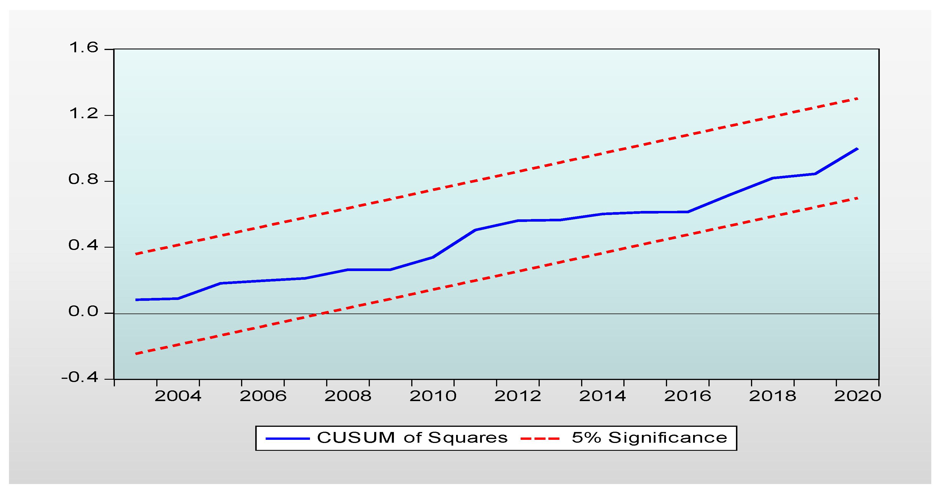
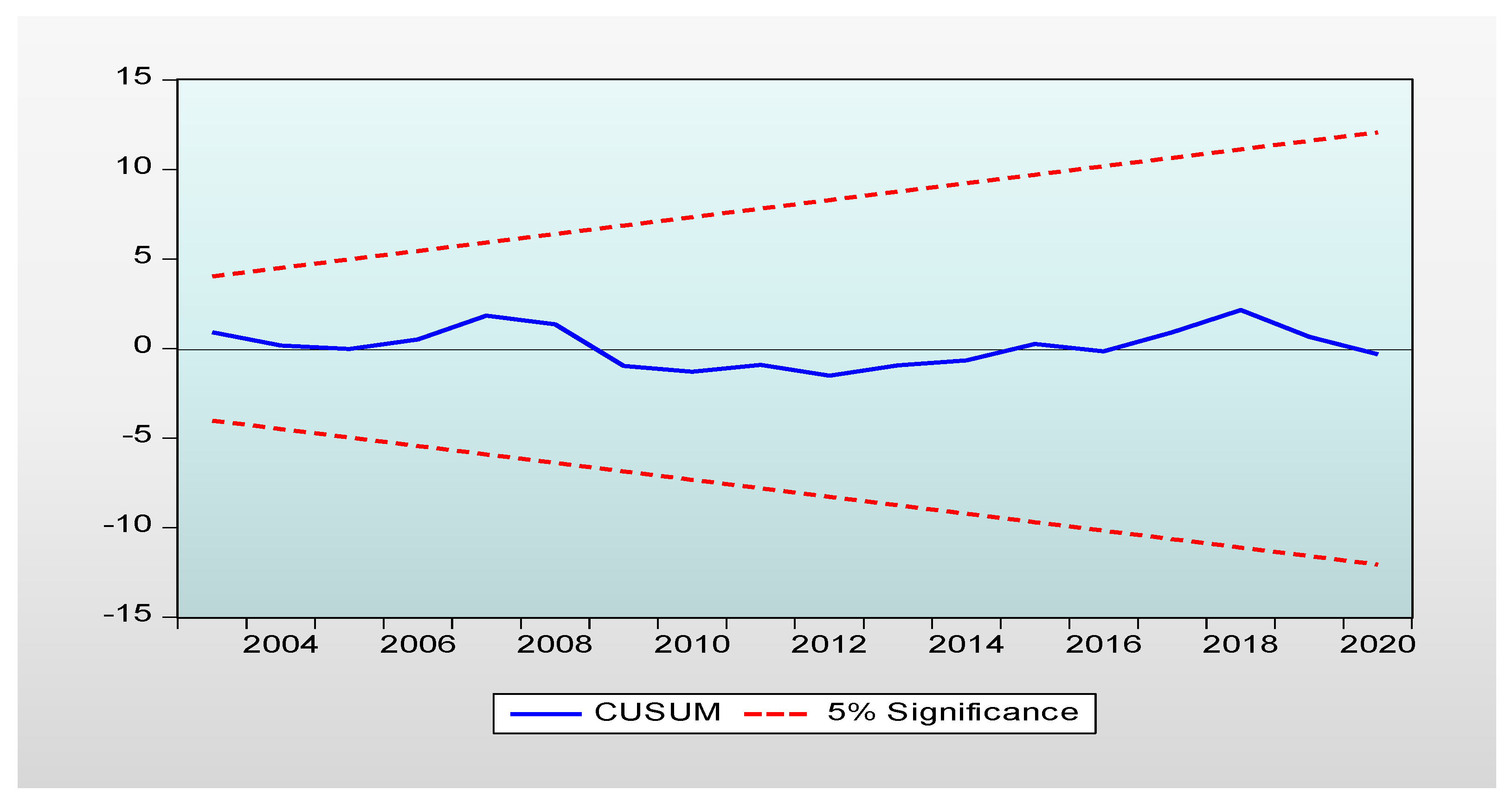
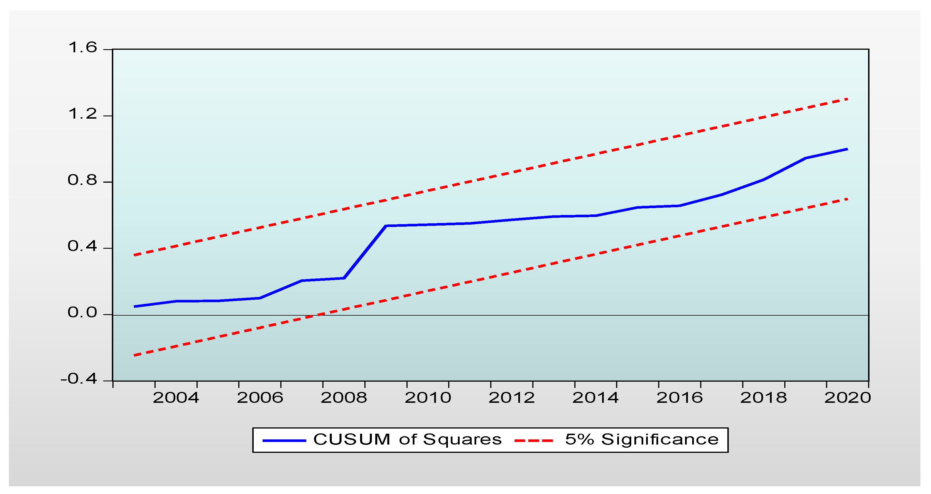
5. Conclusions and Policy Options

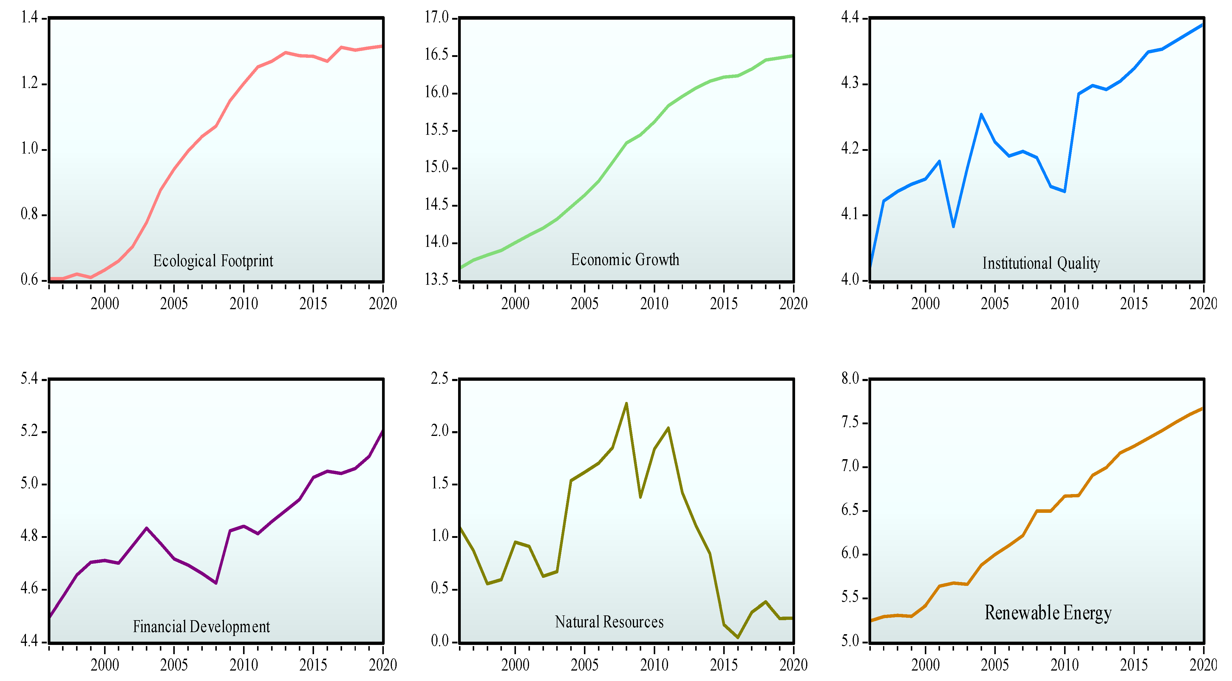
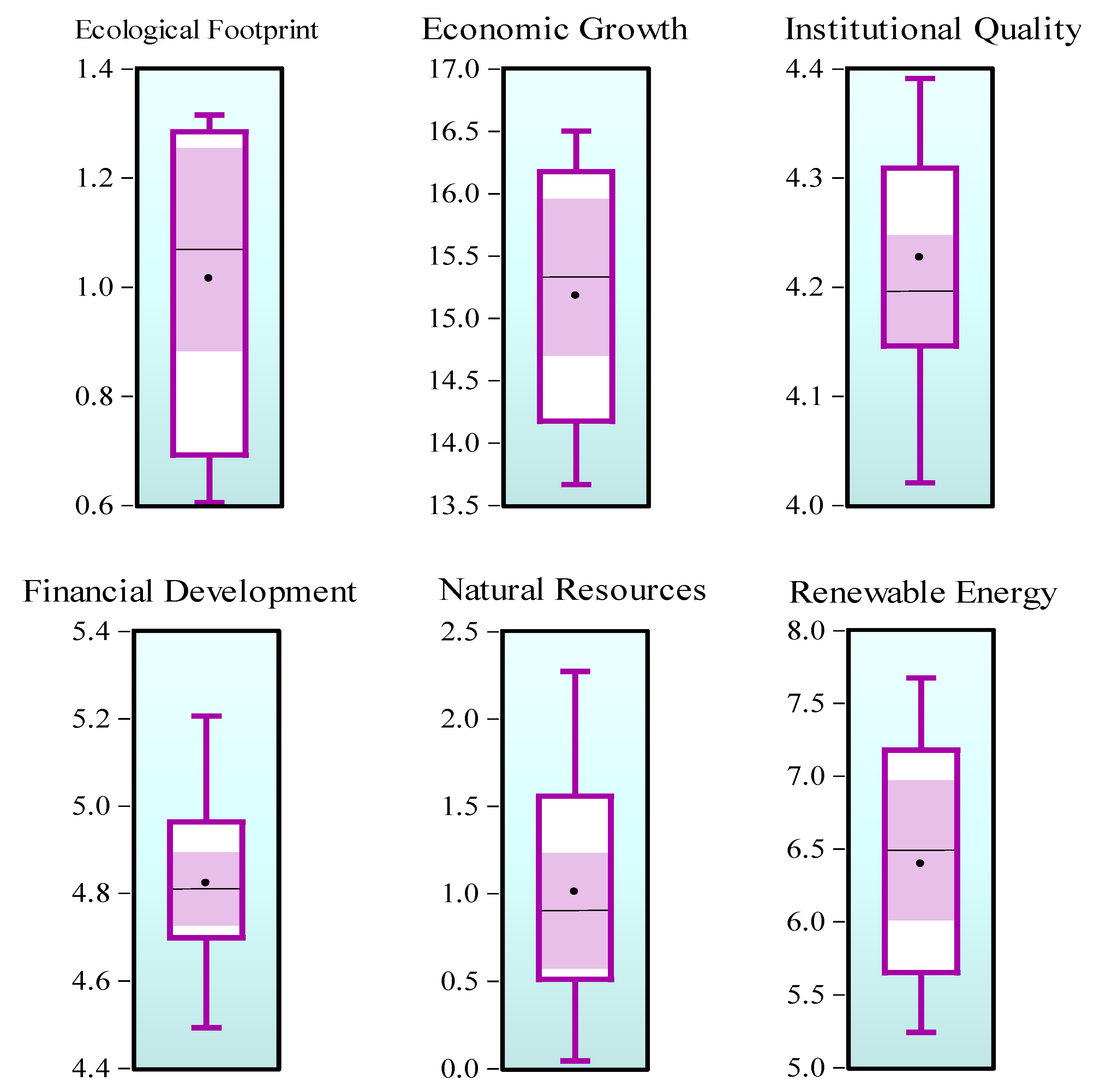
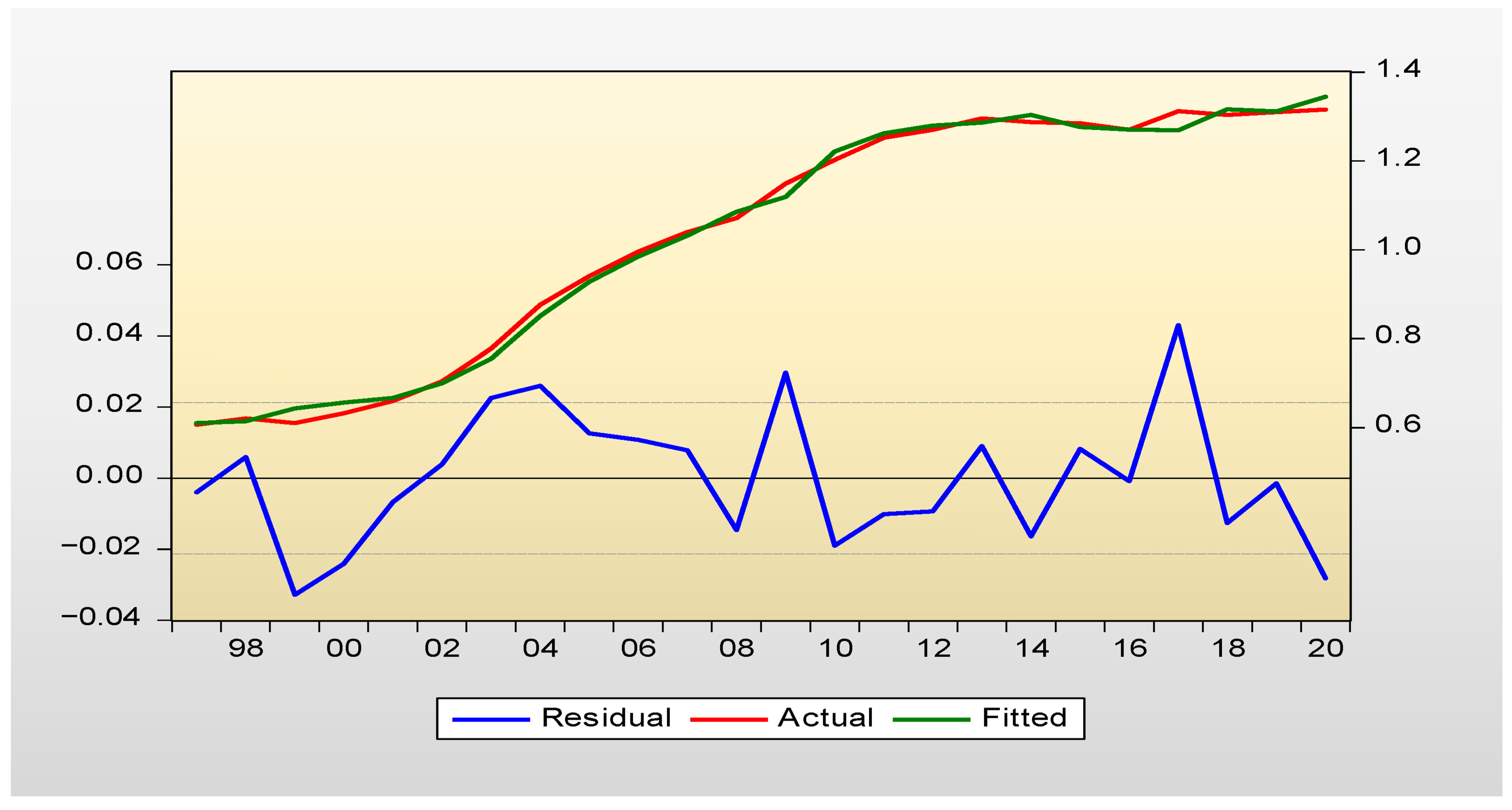
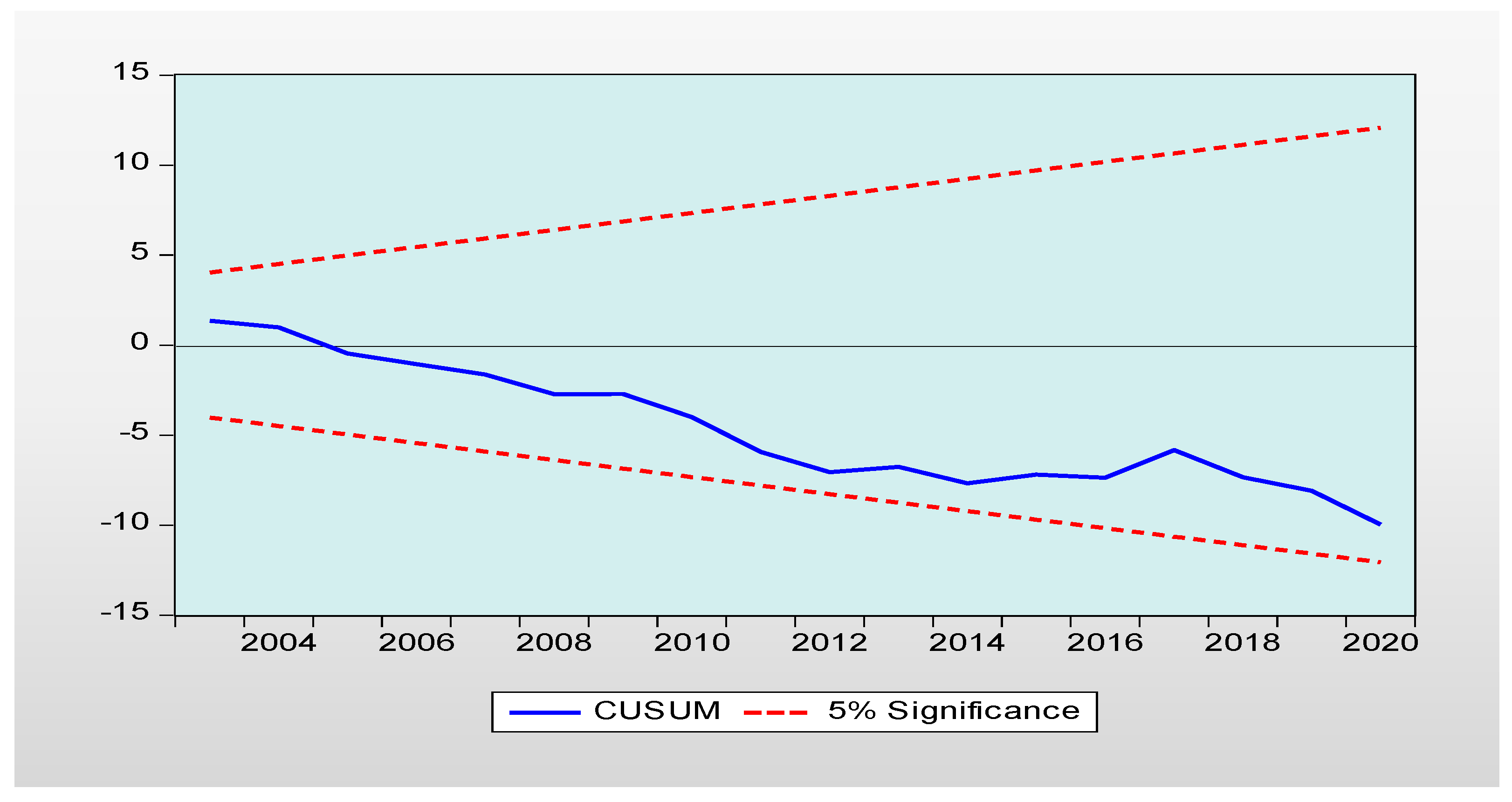
This study examines the long-term, short-term and dynamic influence of institutional quality, natural resources, financial development, and renewable and alternative energy use on economic growth and the environment simultaneously in China, employing series data from 1996 to 2020. To the best of the authors’ knowledge, no earlier research has examined this link in the Chinese context. The Johansen and ARDL bound long-run cointegration approaches were applied to discover the cointegration relationship. Both methods confirm that long-term cointegration was apparent among institutional quality, natural resources, GDP growth, financial expansion, renewable energy, and ecological footprint. The empirical outcomes of the ARDL test show that institutional quality and renewable and clean energy help to protect environmental quality. However, financial progress and total natural resources reduce environmental quality, showing that institutional quality and alternative energy deployment can play a crucial role in diminishing environmental damage in an economy. Further, healthy and sound development in the financial sector can make more funding available at a cheap rate (as the financial markets and institutions are dominated by industrial banks that play a major role in offering credits to both private and public sectors for a variety of developmental ventures) for speculation in ecological projects.

Moreover, all the candidate variables significantly increase economic growth in the long term. In this scenario, when the prospect of the demand for carbon emission protuberance is measured, the significance of financial markets and institutions should also be included as functions of traditional indicators, for instance, energy and income. In addition, an augmentation of alternative and green energy deployment can assist in diminishing ecological damage in China. The findings of the Granger causality method show a two-way causal association between ecological footprint and economic growth. Besides this, there is evidence of a unidirectional causal association from natural resources toward economic growth and institutional quality to the ecological footprint in China.

Based on the above empirical findings, the current research suggests some appropriate policy inferences, as follows: (i) The government of China must be cautious when redesigning economic growth strategies that will make ecological sustainability vulnerable at the national level. (ii) The overall energy mix must be transformed by replacing the fossil fuel energy sources with alternative and renewable energy deployment, since green power sources aid in diminishing ecological damages in China. (iii) Well-developed and advanced carbon trading institutions and markets for public–private partnerships in environmental finance hasten the development and research, and the organization, of a nationwide integrated environmental pollution scheme. This develops a market structure based on active ecological exchanges across China, which enables pilot cities, provinces, and regions to institute their own emissions, authorize allotment schemes/systems and trading methods, and ascertain district emission trading proposals by sharing municipal and provincial information. It also helps establish economic commissions, power preservation, and pollution diminution groups, and advances some other key sectors; consequently, China’s carbon pricing authority can be developed as soon as possible to encourage low-carbon industrial development. In addition, this will vigorously support the R&D of low-carbon technology, which is amongst the main indicators in China’s evolution to a low-carbon nation. This will help in developing new technologies for green growth, reducing coal and gas power consumption, advancing CO₂ storage and capture, develop circular systems for all sectors, thus building up a circular economy, and dynamically endorsing household and industrial waste reprocessing.

The present research features some restrictions and limitations, and formulates suggestions for upcoming research. The first caveat of the present research is the use of EFP as the explained series. In upcoming studies, all sub-components of the ecological footprint must be determined as explained variables, and their link with institutional quality, financial development, natural resources, and renewable energy should be investigated. Second, this study has applied only the time series approach. In upcoming studies, the influence of financial development, institutional quality, natural resources, and renewable energy on a universal scale can be examined by employing panel nonlinear and dynamic ARDL. Third, this study was majorly constrained by data availability (1996 to 2020); upcoming research should increase the data size of these variables. In the end, findings derived from novel econometric approaches and vast data ranges can be compared to those of this study.

References

1. Teng, Y. Tourism, Economic Growth and Sustainable Development in China. Ph.D. Thesis, University of Portsmouth, Portsmouth, UK, 2021. Available online: https://pure.port.ac.uk/ws/portalfiles/portal/49872875/Thesis_1221.docx.pdf (accessed on 3 September 2022).
2. Song, J.; Li, W.H. Countermeasures for the industrial transformation of resource-based cities in heilongjiang province—Based on the discussion of “resource curse” areas. Commer. Econ. 2019, 9, 7–8. [Google Scholar]
3. Khan, H.; Weili, L.; Khan, I. Institutional quality, financial development and the influence of environmental factors on carbon emissions: Evidence from a global perspective. Environ. Sci. Pollut. Res. 2022, 29, 13356–13368. [Google Scholar] [CrossRef] [PubMed]
4. Pan, Y.; Ma, L.; Tang, H.; Wu, Y.; Yang, Z. Land use transitions under rapid urbanization in Chengdu-Chongqing Region: A perspective of coupling water and land resources. Land 2021, 10, 812. [Google Scholar] [CrossRef]
5. Sachs, J.D.; Warner, A.M. Natural Resource Abundance and Economic Growth; NBER Working Paper 5398; National Bureau of Economic Research: Cambridge, MA, USA, 1995. [Google Scholar] [CrossRef]
6. Norman, C.S. Rule of law and the resource curse: Abundance versus intensity. Environ. Resour. Econ. 2009, 43, 183–207. [Google Scholar] [CrossRef]
7. Mehmood, U.; Tariq, S.; Ul-Haq, Z.; Meo, M.S. Does the modifying role of institutional quality remains homogeneous in GDP-CO2 emission nexus? New evidence from ARDL approach. Environ. Sci. Pollut. Res. 2021, 28, 10167–10174. [Google Scholar] [CrossRef]
8. Ahmad, M.; Ahmed, Z.; Yang, X.; Hussain, N.; Sinha, A. Financial development and environmental degradation: Do human capital and institutional quality make a difference? Gondwana Res. 2022, 105, 299–310. [Google Scholar] [CrossRef]
9. Zapata-Cantu, L.; González, F. Challenges for innovation and sustainable development in Latin America: The significance of institutions and human capital. Sustainability 2021, 13, 4077. [Google Scholar] [CrossRef]
10. Ross, M.L. Timber Booms and Institutional Breakdown in Southeast Asia; Cambridge University Press: Cambridge, UK, 2001. [Google Scholar]
11. Acemoglu, D.; Johnson, S.; Robinson, J.A. The colonial origins of comparative development: An empirical investigation. Am. Econ. Rev. 2001, 91, 1369–1401. [Google Scholar] [CrossRef]
12. Zhang, H.; Cong, C.; Chakraborty, A. Exploring the institutional dilemma and governance transformation in China’s urban regeneration: Based on the case of Shanghai Old Town. Cities 2022, 131, 103915. [Google Scholar] [CrossRef]
13. Li, C.; Wan, J.; Xu, Z.; Lin, T. Impacts of green innovation, institutional constraints and their interactions on high-quality economic development across China. Sustainability 2021, 13, 5277. [Google Scholar] [CrossRef]
14. Zahoor, Z.; Latif, M.I.; Khan, I.; Hou, F. Abundance of natural resources and environmental sustainability: The roles of manufacturing value-added, urbanization, and permanent cropland. Environ. Sci. Pollut. Res. 2022, 1–14. [Google Scholar] [CrossRef] [PubMed]
15. Stern, D.I. The role of energy in economic growth. Ann. N. Y. Acad. Sci. 2011, 1219, 26–51. [Google Scholar] [CrossRef] [PubMed]
16. Apergis, N.; Payne, J.E. Renewable energy consumption and economic growth: Evidence from a panel of OECD countries. Energy Policy 2010, 38, 656–660. [Google Scholar] [CrossRef]
17. Jamil, M.N. Critical analysis of energy consumption and its impact on countries economic growth: An empirical analysis base on countries income level. J. Environ. Sci. Econ. 2022, 1, 1–12. [Google Scholar] [CrossRef]
18. Ji, K.; Magnus, J.R.; Wang, W. Natural resources, institutional quality, and economic growth in China. Environ. Resour. Econ. 2013, 57, 323–343. [Google Scholar] [CrossRef]
19. Asghar, N.; Qureshi, D.S.; Nadeem, M. Institutional quality and economic growth: Panel ARDL analysis for selected developing economies of Asia. South Asian Stud. 2020, 30. Available online: http://journals.pu.edu.pk/journals/index.php/IJSAS/article/view/3028 (accessed on 20 August 2022).
20. Nguyen, C.P.; Su, T.D.; Nguyen, T.V.H. Institutional quality and economic growth: The case of emerging economies. Theor. Econ. Lett. 2018, 8, 1943. [Google Scholar] [CrossRef] [Green Version]
21. Poshakwale, S.; Ganguly, G. International shocks and growth in emerging markets. Glob. Financ. J. 2015, 26, 29–46. [Google Scholar] [CrossRef] [Green Version]
22. Chan, S.G.; Koh, E.H.; Zainir, F.; Yong, C.C. Market structure, institutional framework and bank efficiency in ASEAN 5. J. Econ. Bus. 2015, 82, 84–112. [Google Scholar] [CrossRef]
23. Wu, H.; Ren, S.; Xie, G. Technology Import and China’s Innovation Capability: Does Institutional Quality Matter? Reg. Econ. Dev. Res. 2020, 1, 93. Available online: https://papers.ssrn.com/sol3/papers.cfm?abstract_id=3811595 (accessed on 23 August 2022).
24. Peres, M.; Ameer, W.; Xu, H. The impact of institutional quality on foreign direct investment inflows: Evidence for developed and developing countries. Econ. Res.-Ekon. Istraživanja 2018, 31, 626–644. [Google Scholar] [CrossRef] [Green Version]
25. Qiang, Q.; Jian, C. Natural resource endowment, institutional quality and China’s regional economic growth. Resour. Policy 2020, 66, 101644. [Google Scholar] [CrossRef]
26. Tsani, S. Natural resources, governance and institutional quality: The role of resource funds. Resour. Policy 2013, 38, 181–195. [Google Scholar] [CrossRef]
27. Shuai, S.; Qi, Z. Energy exploitation and economic growth in Western China: An empirical analysis based on the resource curse hypothesis. Front. Econ. China 2009, 4, 125–152. [Google Scholar]
28. Jalil, A.; Feridun, M. The impact of growth, energy and financial development on the environment in China: A cointegration analysis. Energy Econ. 2011, 33, 284–291. [Google Scholar] [CrossRef]
29. Al-Mulali, U.; Tang, C.F.; Ozturk, I. Does financial development reduce environmental degradation? Evidence from a panel study of 129 countries. Environ. Sci. Pollut. Res. 2015, 22, 14891–14900. [Google Scholar] [CrossRef] [PubMed]
30. Adebanjo, S.A.; Shakiru, T.H. Dynamic relationship between air pollution and economic growth in Jordan: An empirical analysis. J. Environ. Sci. Econ. 2022, 1, 30–43. [Google Scholar] [CrossRef]
31. Boutabba, M.A. The impact of financial development, income, energy and trade on carbon emissions: Evidence from the Indian economy. Econ. Model. 2014, 40, 33–41. [Google Scholar] [CrossRef] [Green Version]
32. Omri, A.; Daly, S.; Rault, C.; Chaibi, A. Financial development, environmental quality, trade and economic growth: What causes what in MENA countries. Energy Econ. 2015, 48, 242–252. [Google Scholar] [CrossRef] [Green Version]
33. Zaidi, S.A.H.; Zafar, M.W.; Shahbaz, M.; Hou, F. Dynamic linkages between globalization, financial development and carbon emissions: Evidence from Asia Pacific Economic Cooperation countries. J. Clean. Prod. 2019, 228, 533–543. [Google Scholar] [CrossRef]
34. Hartwick, J.M. Intergenerational equity and the investing of rents from exhaustible resources. In The Economics of Sustainability; Routledge: London, UK, 2017; pp. 63–65. Available online: https://www.taylorfrancis.com/chapters/edit/10.4324/9781315240084-4/intergenerational-equity-investing-rents-exhaustible-resources-john-hartwick (accessed on 3 September 2022).
35. Baloch, M.A.; Mahmood, N.; Zhang, J.W. Effect of natural resources, renewable energy and economic development on CO2 emissions in BRICS countries. Sci. Total Environ. 2019, 678, 632–638. [Google Scholar] [CrossRef]
36. Adebanjo, S.A.; Adeoye, O.M. Transparency and Global Initiatives in the Face of Natural Resource Depletion in Sub-Saharan Africa. J. Environ. Sci. Econ. 2022, 1, 15–29. [Google Scholar] [CrossRef]
37. Jahanger, A.; Usman, M.; Balsalobre-Lorente, D. Linking institutional quality to environmental sustainability. Sustain. Dev. 2022, 1–19. [Google Scholar] [CrossRef]
38. Dagar, V.; Khan, M.K.; Alvarado, R.; Rehman, A.; Irfan, M.; Adekoya, O.B.; Fahad, S. Impact of renewable energy consumption, financial development and natural resources on environmental degradation in OECD countries with dynamic panel data. Environ. Sci. Pollut. Res. 2022, 29, 18202–18212. [Google Scholar] [CrossRef] [PubMed]
39. Epo, B.N.; Faha, D.R.N. Natural resources, institutional quality, and economic growth: An African tale. Eur. J. Dev. Res. 2020, 32, 99–128. [Google Scholar] [CrossRef]
40. Egbetokun, S.; Osabuohien, E.; Akinbobola, T.; Onanuga, O.T.; Gershon, O.; Okafor, V. Environmental pollution, economic growth and institutional quality: Exploring the nexus in Nigeria. Manag. Environ. Qual. Int. J. 2019, 31, 18–31. [Google Scholar] [CrossRef] [Green Version]
41. Khan, M.A.; Gu, L.; Khan, M.A.; Oláh, J. Natural resources and financial development: The role of institutional quality. J. Multinatl. Financ. Manag. 2020, 56, 100641. [Google Scholar] [CrossRef]
42. Godil, D.I.; Sharif, A.; Agha, H.; Jermsittiparsert, K. The dynamic nonlinear influence of ICT, financial development, and institutional quality on CO2 emission in Pakistan: New insights from QARDL approach. Environ. Sci. Pollut. Res. 2020, 27, 24190–24200. [Google Scholar] [CrossRef]
43. Elsalih, O.; Sertoglu, K.; Besim, M. Environmental performance, comparative advantage of crude oil and the role of institutional quality. Environ. Sci. Pollut. Res. 2020, 27, 3489–3496. [Google Scholar] [CrossRef]
44. Yousaf, U.S.; Ali, F.; Aziz, B.; Sarwar, S. What causes environmental degradation in Pakistan? Embossing the role of fossil fuel energy consumption in the view of ecological footprint. Environ. Sci. Pollut. Res. 2022, 29, 33106–33116. [Google Scholar] [CrossRef]
45. Usman, M.; Jahanger, A. Heterogeneous effects of remittances and institutional quality in reducing environmental deficit in the presence of EKC hypothesis: A global study with the application of panel quantile regression. Environ. Sci. Pollut. Res. 2021, 28, 37292–37310. [Google Scholar] [CrossRef] [PubMed]
46. Khan, H.; Weili, L.; Khan, I. The role of institutional quality in FDI inflows and carbon emission reduction: Evidence from the global developing and belt road initiative countries. Environ. Sci. Pollut. Res. 2022, 29, 30594–30621. [Google Scholar] [CrossRef] [PubMed]
47. Ayad, H.; Sari-Hassoun, S.E.; Usman, M.; Ahmad, P. The impact of economic uncertainty, economic growth and energy consumption on environmental degradation in MENA countries: Fresh insights from multiple thresholds NARDL approach. Environ. Sci. Pollut. Res. 2022, 1–19. [Google Scholar] [CrossRef] [PubMed]
48. Ahmad, M.; Ahmed, Z.; Majeed, A.; Huang, B. An environmental impact assessment of economic complexity and energy consumption: Does institutional quality make a difference? Environ. Impact Assess. Rev. 2021, 89, 106603. [Google Scholar] [CrossRef]
49. Zhang, Y.J.; Jin, Y.L.; Chevallier, J.; Shen, B. The effect of corruption on carbon dioxide emissions in APEC countries: A panel quantile regression analysis. Technol. Forecast. Soc. Chang. 2016, 112, 220–227. [Google Scholar] [CrossRef]
50. Zakaria, M.; Bibi, S. Financial development and environment in South Asia: The role of institutional quality. Environ. Sci. Pollut. Res. 2019, 26, 7926–7937. [Google Scholar] [CrossRef] [PubMed]
51. Ali, M.; Nazir, M.I.; Hashmi, S.H.; Ullah, W. Financial inclusion, institutional quality and financial development: Empirical evidence from OIC countries. Singap. Econ. Rev. 2022, 67, 161–188. [Google Scholar] [CrossRef]
52. Usman, M.; Balsalobre-Lorente, D. Environmental concern in the era of industrialization: Can financial development, renewable energy and natural resources alleviate some load? Energy Policy 2022, 162, 112780. [Google Scholar] [CrossRef]
53. Aslan, A.; Altinoz, B. The impact of natural resources and gross capital formation on economic growth in the context of globalization: Evidence from developing countries on the continent of Europe, Asia, Africa, and America. Environ. Sci. Pollut. Res. 2021, 28, 33794–33805. [Google Scholar] [CrossRef]
54. Zafar, M.W.; Saeed, A.; Zaidi, S.A.H.; Waheed, A. The linkages among natural resources, renewable energy consumption, and environmental quality: A path toward sustainable development. Sustain. Dev. 2021, 29, 353–362. [Google Scholar] [CrossRef]
55. Pata, U.K.; Caglar, A.E. Investigating the EKC hypothesis with renewable energy consumption, human capital, globalization and trade openness for China: Evidence from augmented ARDL approach with a structural break. Energy 2021, 216, 119220. [Google Scholar] [CrossRef]
56. Usman, M.; Radulescu, M. Examining the role of nuclear and renewable energy in reducing carbon footprint: Does the role of technological innovation really create some difference? Sci. Total Environ. 2022, 841, 156662. [Google Scholar] [CrossRef]
57. Langnel, Z.; Amegavi, G.B. Globalization, electricity consumption and ecological footprint: An autoregressive distributive lag (ARDL) approach. Sustain. Cities Soc. 2020, 63, 102482. [Google Scholar] [CrossRef]
58. Phillips, P.C. Understanding spurious regressions in econometrics. J. Econ. 1986, 33, 311–340. [Google Scholar] [CrossRef] [Green Version]
59. Phillips, P.C.; Perron, P. Testing for a unit root in time series regression. Biometrika 1988, 75, 335–346. [Google Scholar] [CrossRef]
60. Dickey, D.A.; Fuller, W.A. Distribution of the estimators for autoregressive time series with a unit root. J. Am. Stat. Assoc. 1979, 74, 427–431. [Google Scholar] [CrossRef]
61. Kwiatkowski, D.; Phillips, P.C.; Schmidt, P.; Shin, Y. Testing the null hypothesis of stationarity against the alternative of a unit root: How sure are we that economic time series have a unit root? J. Econom. 1992, 54, 159–178. [Google Scholar] [CrossRef]
62. Pao, H.T.; Tsai, C.M. Modeling and forecasting the CO2 emissions, energy consumption, and economic growth in Brazil. Energy 2011, 36, 2450–2458. [Google Scholar] [CrossRef]
63. Johansen, S. Statistical analysis of cointegration vectors. J. Econ. Dyn. Control 1988, 12, 231–254. [Google Scholar] [CrossRef]
64. Ivascu, L.; Sarfraz, M.; Mohsin, M.; Naseem, S.; Ozturk, I. The causes of occupational accidents and injuries in Romanian firms: An application of the Johansen cointegration and Granger causality test. Int. J. Environ. Res. Public Health 2021, 18, 7634. [Google Scholar] [CrossRef]
65. Pesaran, M.H.; Shin, Y.; Smith, R.J. Bounds testing approaches to the analysis of level relationships. J. Appl. Econom. 2001, 16, 289–326. [Google Scholar] [CrossRef]
66. Samantaraya, A.; Patra, S.K. Determinants of household savings in India: An empirical analysis using ARDL approach. Econ. Res. Int. 2014, 2014, 1–8. [Google Scholar] [CrossRef]
67. Sun, C.; Zhang, F.; Xu, M. Investigation of pollution haven hypothesis for China: An ARDL approach with breakpoint unit root tests. J. Clean. Prod. 2017, 161, 153–164. [Google Scholar] [CrossRef]
68. Granger, C.W.J. Investigating causal relations by econometric models and cross-spectral methods. Econometrica 1969, 37, 424–438. [Google Scholar] [CrossRef]
69. Sarkodie, S.A.; Adams, S. Renewable energy, nuclear energy, and environmental pollution: Accounting for political institutional quality in South Africa. Sci. Total Environ. 2018, 643, 1590–1601. [Google Scholar] [CrossRef]
70. Farhani, S.; Ozturk, I. Causal relationship between CO2 emissions, real GDP, energy consumption, financial development, trade openness, and urbanization in Tunisia. Environ. Sci. Pollut. Res. 2015, 22, 15663–15676. [Google Scholar] [CrossRef]
71. Ehigiamusoe, K.U.; Lean, H.H.; Babalola, S.J.; Poon, W.C. The roles of financial development and urbanization in degrading environment in Africa: Unraveling nonlinear and moderating impacts. Energy Rep. 2022, 8, 1665–1677. [Google Scholar] [CrossRef]
72. Acheampong, A.O. Modelling for insight: Does financial development improve environmental quality? Energy Econ. 2019, 83, 156–179. [Google Scholar] [CrossRef]
73. Ibrahiem, D.M. Do technological innovations and financial development improve environmental quality in Egypt? Environ. Sci. Pollut. Res. 2020, 27, 10869–10881. [Google Scholar] [CrossRef]
74. Baloch, M.A.; Ozturk, I.; Bekun, F.V.; Khan, D. Modeling the dynamic linkage between financial development, energy innovation, and environmental quality: Does globalization matter? Bus. Strategy Environ. 2021, 30, 176–184. [Google Scholar] [CrossRef]
75. Wang, L.; Vo, X.V.; Shahbaz, M.; Ak, A. Globalization and carbon emissions: Is there any role of agriculture value-added, financial development, and natural resource rent in the aftermath of COP21? J. Environ. Manag. 2020, 268, 110712. [Google Scholar] [CrossRef] [PubMed]
76. Danish; Ulucak, R.; Khan, S.U.D. Determinants of the ecological footprint: Role of renewable energy, natural resources, and urbanization. Sustain. Cities Soc. 2020, 54, 101996. [Google Scholar] [CrossRef]
77. Ibrahim, R.L.; Ajide, K.B.; Usman, M.; Kousar, R. Heterogeneous effects of renewable energy and structural change on environmental pollution in Africa: Do natural resources and environmental technologies reduce pressure on the environment? Renew. Energy 2022, 1–19. [Google Scholar] [CrossRef]
78. Dong, K.; Sun, R.; Jiang, H.; Zeng, X. CO2 emissions, economic growth, and the environmental Kuznets curve in China: What roles can nuclear energy and renewable energy play? J. Clean. Prod. 2018, 196, 51–63. [Google Scholar] [CrossRef]
79. Lajqi, S.; Krasniqi, B.A. Entrepreneurial growth aspirations in challenging environment: The role of institutional quality, human and social capital. Strateg. Chang. 2017, 26, 385–401. [Google Scholar] [CrossRef]
80. Bhattacharya, M.; Churchill, S.A.; Paramati, S.R. The dynamic impact of renewable energy and institutions on economic output and CO2 emissions across regions. Renew. Energy 2017, 111, 157–167. [Google Scholar] [CrossRef]
81. Jović, S.; Maksimović, G.; Jovović, D. Appraisal of natural resources rents and economic development. Resour. Policy 2016, 50, 289–291. [Google Scholar] [CrossRef]
82. Shao, S.; Yang, L. Natural resource dependence, human capital accumulation, and economic growth: A combined explanation for the resource curse and the resource blessing. Energy Policy 2014, 74, 632–642. [Google Scholar] [CrossRef]
83. Brunnschweiler, C.N.; Bulte, E.H. The resource curse revisited and revised: A tale of paradoxes and red herrings. J. Environ. Econ. Manag. 2008, 55, 248–264. [Google Scholar] [CrossRef] [Green Version]
84. Pao, H.T.; Fu, H.C. Renewable energy, non-renewable energy and economic growth in Brazil. Renew. Sustain. Energy Rev. 2013, 25, 381–392. [Google Scholar] [CrossRef]
85. Salman, M.; Long, X.; Dauda, L.; Mensah, C.N. The impact of institutional quality on economic growth and carbon emissions: Evidence from Indonesia, South Korea and Thailand. J. Clean. Prod. 2019, 241, 118331. [Google Scholar] [CrossRef]
86. Amin, M.; Djankov, S. Natural resources and reforms. Available at SSRN 1366034. Available online: https://papers.ssrn.com/sol3/papers.cfm?abstract_id=1366034 (accessed on 21 September 2022).
87. Mehlum, H.; Moene, K.; Torvik, R. Institutions and the resource curse. Econ. J. 2006, 116, 1–20. [Google Scholar] [CrossRef] [Green Version]
88. Chandio, A.A.; Sethi, N.; Dash, D.P.; Usman, M. Towards sustainable food production: What role ICT and technological development can play for cereal production in Asian–7 countries? Comput. Electron. Agric. 2022, 202, 107368. [Google Scholar] [CrossRef]
Figure 1. Trend analysis of analyzed variables.
Sustainability 14 13910 g001
Figure 2. Box chart summary of selected variables.
Sustainability 14 13910 g002
Figure 3. Actual, fitted, and residual plot of the ecological footprint function.
Sustainability 14 13910 g003
Figure 4. Actual, fitted, and residual plot of the economic growth footprint function.
Sustainability 14 13910 g004
Figure 5. The cumulative sum of the recursive residual plot (EFP function).
Sustainability 14 13910 g005
Figure 6. The cumulative sum of the square of the recursive residual plot (EFP function).
Sustainability 14 13910 g006
Figure 7. The cumulative sum of the recursive residual plot (GDP function).
Sustainability 14 13910 g007
Figure 8. The cumulative sum of the square of the recursive residual plot (GDP function).
Sustainability 14 13910 g008