Retinal stem cells modulate proliferative parameters to coordinate post-embryonic morphogenesis in the eye of fish
- Heidelberg University, Germany
Figures
Figure 1 with 2 supplements

Clonal labelling enables analysis of growth patterns in NR and RPE.
(A) Schematic anatomy of the fish eye. (B) Growth patterns of retinal cell population (concentric rings) and individual clones. (C) False color immunostained NR of 3 week old Rx2::ERT2Cre, GaudíRSG fish with ArCoS and concentric rings of IdU-labelled cells. Overnight IdU pulses were at 1 and 2.5 weeks of age. Leftover undissected autofluorescent tissue fragments cover the far right of the cup-shaped retina. (D) Proximal view of clones induced in the NR of Rx2::ERT2Cre, Gaudí2.1 fish. Maximum projection of confocal stack of GFP immunostaining in false colors. (E) Proximal view of unpigmented lineages induced in the RPE by mosaic bi-allelic knockout of Oca2 using CRISPR/Cas9. Focused projection of brightfield focal stack. Images in (D) and (E) have been rotated to place the optic nerve exit (pink asterisk) ventrally; the embryonic retina is circled with a pink dashed line.
Figure 1—figure supplement 1
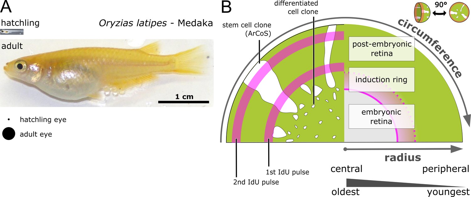
The retinal radius represents a temporal axis.
(A) Photos of newly hatched and young sexually mature adult medaka. The projected area of hatchling and adult eyes is highlighted underneath. (B) Schematic drawing of proximal view on clones and IdU ‘growth rings’ of the NR. The central part of the eye is formed embryonically and contains the oldest cells, while the post-embryonic retina is younger and derives from stem cells in the CMZ, which is located at the extreme periphery. The embryonic retina corresponds to the area of the entire differentiated retina in the hatchling; the induction ring corresponds to the position of the CMZ at the timepoint of Cre recombination.
Figure 1—figure supplement 2
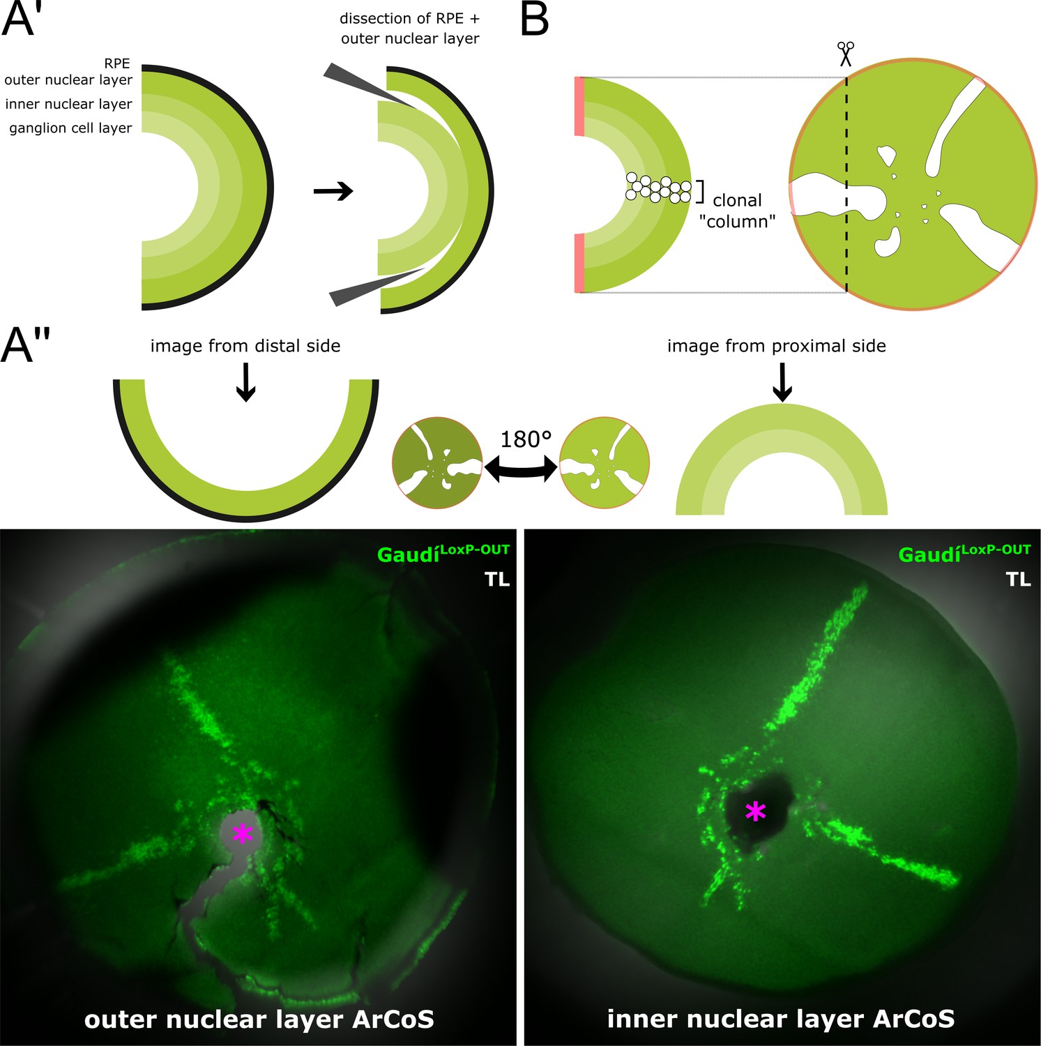
NR ArCoS form narrow columns spanning all NR layers.
(A’) Schematic cross-section of a dissected retina illustrating the various neuronal layers of the NR. The RPE is single-layered. With short fixation times and careful dissection, the RPE and outer nuclear layer can be peeled off from the inner nuclear and ganglion cell layers. (A’’) Retina dissected from an adult fish that received a transplant of cells from ubiquitously GFP-expressing donors (GaudíLoxP-OUT) at embryonic blastula stage. NR clones always span all neuronal layers throughout the retinal radius. Maximum projection of confocal stacks of different preparations of the same retina showing endogenous GFP signal and transmitted light (TL). Pink asterisk marks optic nerve exit. (B) Schematic cross-section through an NR ArCoS highlighting clonal columns among differentiated retinal progeny.
Figure 2 with 3 supplements

Feedback between proliferation and organ growth affects the simulated clonal pattern.
(A) Initial condition and properties of the agent based model of the growing fish retina. Virtual embryonic retina in light green. CMZ cells are assigned unique colors for virtual clonal analysis. (B’) Simulated IdU pulse-chase experiment. First pulse: 200–220 hr, second pulse: 400–420 hr. Screenshot from 435 hr. Virtual cells incorporate IdU when they divide and half of the signal is passed on to each daughter cell. (B’’) Cell age (hours elapsed since last cell division) forms a gradient with the oldest cells in the virtual embryonic retina. (C’) In the inducer growth mode, the modelled tissue signals upstream to drive growth of other tissues in the organ. (C’’) Representative screenshot of inducer growth mode. (C’’’) Sample of 10 clones from (C’’). Colors: ratio of full perimeter by bounding rectangle perimeter, a metric for shape complexity. (C’’’’) Cell division intervals plotted against the mean average overlap. (D’) In the responder growth mode, control of the growth of the modelled tissue is downstream of an external signal. (D’’) Representative screenshot of the responder growth mode. (D’’’) Sample of 10 clones from (D’’) evaluated by the same shape metric as in (C’’’). (D’’’’) Cell division intervals plotted against the mean average overlap. Note the higher range of values for cells over the threshold overlap of 0.2.
Figure 2—figure supplement 1
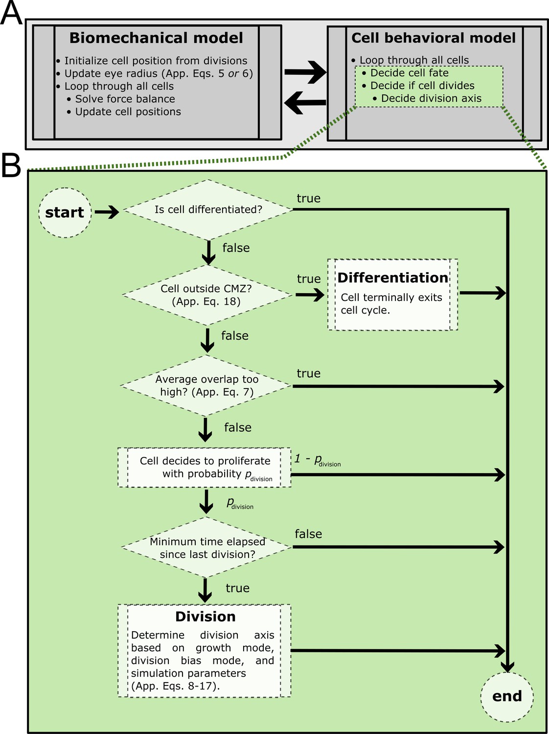
Process diagram summarizing model decision tree.
(A) At every simulation step, the biomechanical model is solved followed by simulation of the cell behavioral model. Green shaded steps expanded in (B). (B) Summary of cell behavioral decision tree. If a cell decides to divide but the minimum cell cycle time has not elapsed, it will suppress division and check only the other conditions (proliferative cell type, permissive overlap, minimum time elapsed).
Figure 2—figure supplement 2

Cell position update with radial growth of the simulated retina.
To simulate radial growth, the vectors extending from the eye globe’s center to the cells’ center are extended to match the radius of the growing hemispherical organ. This leads to a decrease in cell density over time as described for growing fish eyes (Lyall, 1957; Johns, 1977; Ohki and Aoki, 1985). Additionally, every numerical step of the solver for the biomechanical force-balance includes similar repositioning of all cells, to ensure they stay on the hemispherical surface. Each simulation step includes 100 such iterations.
Figure 2—figure supplement 3
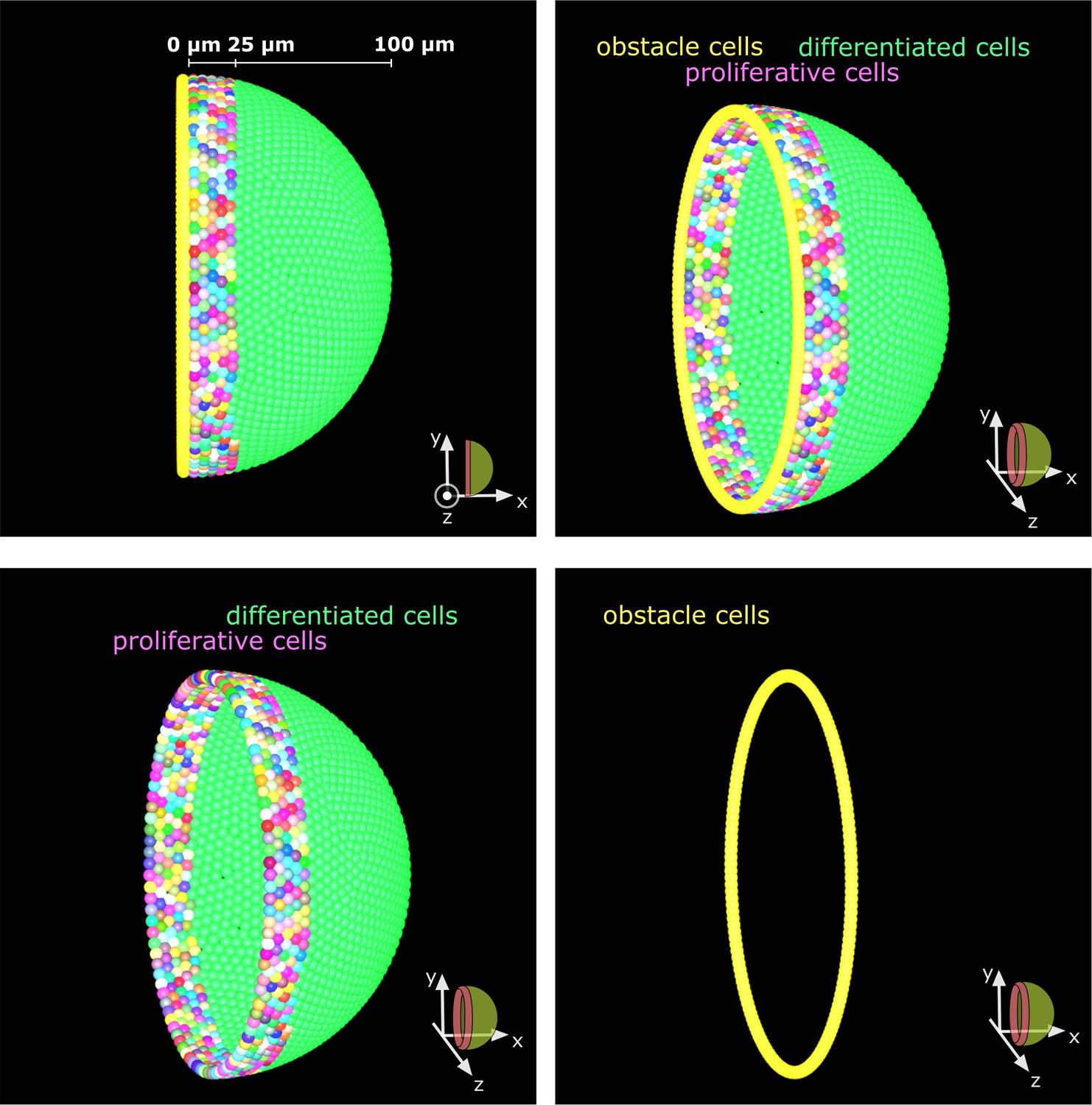
Obstacle cells create an impassable boundary at the hemisphere’s edge.
A single layer of tightly packed cells prevents cell movement beyond the hemispherical edge. These obstacle cells represent the edge of the tissue and have no other influence on the simulation.
Figure 3 with 2 supplements

Cell division variability is lower in NR and inducer growth mode, higher in RPE and responder growth mode.
(A’–A’’) Proximal view of segmented patches in adult NR and RPE and simulated patches in inducer and responder growth mode. The central (virtual) embryonic retina was excluded from analysis. (B) Different degrees of variability in cell division timing affect the clone pattern. (C’–C’’) Upper panels: Superposition of labelled patches in the NR (n = 156 patches from seven retinae), RPE (n = 142 patches from 10 retinae), inducer growth mode (n = 145 patches from five simulations), and responder growth mode (n = 107 patches from five simulations). The radius was normalized to the same length in all samples. Lower panels: Gaussian fits of normalized pixel intensity profiles projected along the vertical axis. σ - Standard deviation of fit. (D) Distribution of number of nodes of skeletonized patches. Inset: Examples of patches without nodes (I), with only one node (II), or with multiple nodes (III). (E) Rug plot showing number of patches that are not connected to the embryonic retina (‘late arising patches’) at the respective positions along the normalized radius. NR (n = 54 late patches) and inducer growth mode (n = 35 late patches) display a marked peak in the central portion, while RPE (n = 56 late patches) and responder growth mode (n = 37 late patches) have a more uniform distribution.
-
Figure 3—source data 1
Patch outlines.
Figure 3C’–C’’ ‘roi’ format files of aligned individual patch outlines for each condition. Data can be opened in the program ‘ImageJ’.
- https://doi.org/10.7554/eLife.42646.016
-
Figure 3—source data 2
Patch superposition.
Figure 3C’–C’’ ‘Tif’ format files of patch superposition, which can be opened in the program ‘ImageJ’. Averaged pixel intensity profiles measured on the patch superposition in ImageJ using the ‘Plot Profile’ function over a rectangle encompassing the entire image.
- https://doi.org/10.7554/eLife.42646.017
-
Figure 3—source data 3
Nodes per patch Figure 3D) Counts of number of nodes in each patch for each condition.
- https://doi.org/10.7554/eLife.42646.018
-
Figure 3—source data 4
Late arising patches Figure 3E) Counts of number of patches along normalized radial bins.
For each patch, the starting position along normalized radial bins was noted. Patches that did not begin in the first radial bin (and thus were not connected to the central embryonic retina) were considered ‘late arising patches’.
- https://doi.org/10.7554/eLife.42646.019
-
Figure 3—source data 5
Comparison of distribution of number of nodes.
Wilcoxon rank sum test applied to the data in Figure 3D rounded to two digits.
- https://doi.org/10.7554/eLife.42646.023
-
Figure 3—source data 6
Comparison of distribution of late arising patches.
Wilcoxon rank sum test applied to the data in Figure 3E rounded to two digits.
- https://doi.org/10.7554/eLife.42646.024
Figure 3—figure supplement 1
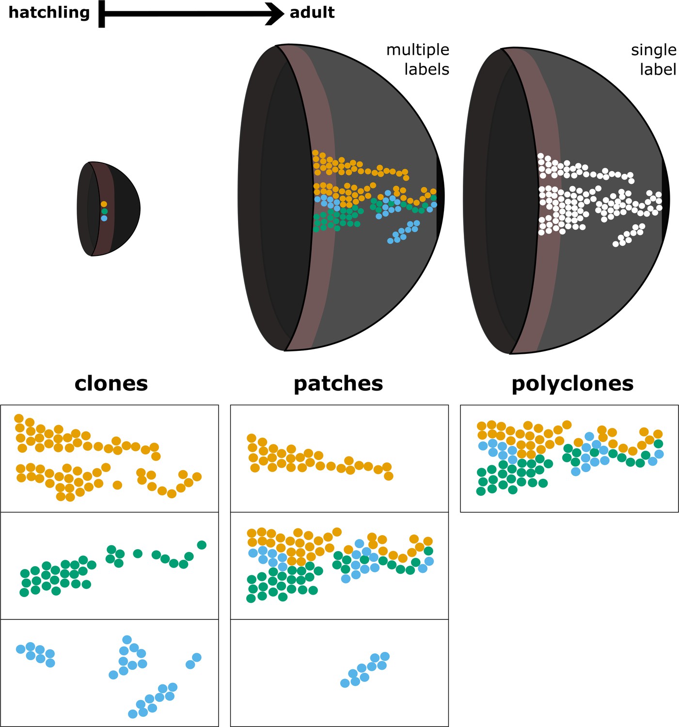
Relationship between clones, patches, and polyclones.
The term clone denotes lineages derived from a single founder cell, while polyclones are conglomerates of clones that are spatially clustered. We define patches as contiguous domains of labelled cells regardless of their clonal relationship. A patch may represent a clone, a fragment of a clone, or a polyclone.
Figure 3—figure supplement 2
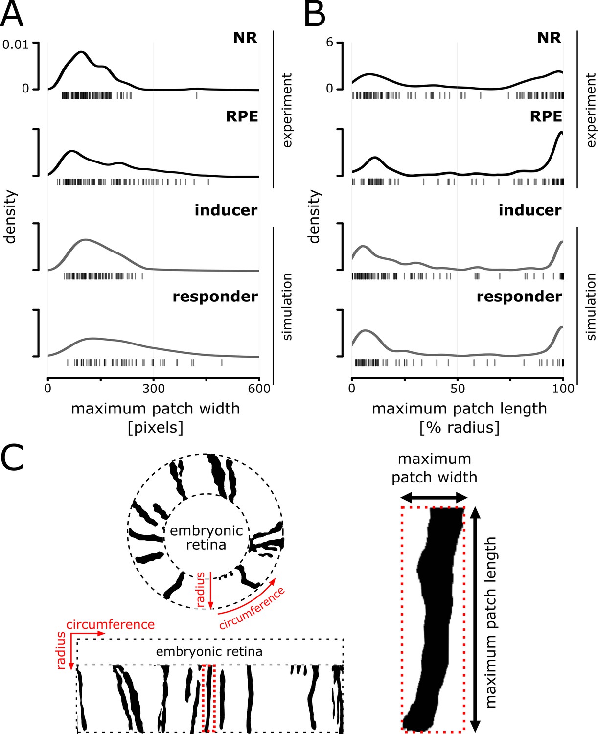
Distributions of patch width and length in experiment and simulation.
(A) Distribution of maximum width of patches that span at least 20% of the radial coordinate. (B) Distribution of maximum patch length normalized against the postembryonic retinal radius; late arising patches (central-most pixel after 20% of the radius) were excluded from the analysis. Note the bimodal distribution that results from the abundance of very short and very long patches. (C) Illustration of a retina before and after transforming from polar coordinates centered on the embryonic retina to a cartesian representation. Patch bordered in dotted red line is magnified on the right to illustrate the metrics used for plotting distributions in (A) and (B) of this figure.
-
Figure 3—figure supplement 2—source data 1
Patch width distribution.
Figure 3—figure supplement 2A) Maximum patch width in pixels for each condition.
- https://doi.org/10.7554/eLife.42646.020
-
Figure 3—figure supplement 2—source data 2
Patch height distribution.
Figure 3—figure supplement 2B) Maximum patch height (expressed as percent of total postembryonic radius) for each condition.
- https://doi.org/10.7554/eLife.42646.021
-
Figure 3—figure supplement 2—source data 3
Comparison of variances of maximum patch width distribution.
F-test of equality of variance applied to the data in Figure 3—figure supplement 2A rounded to two digits.
- https://doi.org/10.7554/eLife.42646.022
Figure 4 with 1 supplement
The majority of stem cells differentiates due to cell competition for niche space.
(A’) Detail of inducer growth mode simulation where clone label was initiated at a radius of R = 100 µm. Small clusters lie centrally, while virtual ArCoS start peripherally. Two virtual ArCoS are highlighted. Pink dashed lines encircle virtual induction ring. (A’’) Same simulation as in (A’), but with clone label initiated at R = 150 µm. The second wave of clonal label leads to a renewed occurrence of small clusters. Two polyclonal patches are highlighted, which correspond to subclones of the highlighted clones in (A’). (B) The majority of virtual ArCoS derives from stem cells that in simulation step 0 were located in the two most peripheral rows of the virtual CMZ. (C’) Proximal view of NR clones. (C’’) Magnification of central retina from (C’). (C’–C’’) Maximum projection of confocal stack of GFP signal in false colors; rotated to place optic nerve exit (pink asterisk) ventrally. (D’) Proximal view of simulated clones. (D’’) Magnification of central retina from (D’). (C’–D’) Retinal edge marked by white dashed circle; dashed pink lines encircle and subdivide induction ring into central and peripheral parts; pink arrowheads mark ArCoS, yellow arrowheads mark terminated clones. (E) Scheme of the experiment. (F) Proportions of ArCoS and terminated clones arising from central and peripheral induction ring in experiment (n = 20 retinae) and simulation (n = 5 simulations, sampled six times each). p-values calculated with a 2-sample test for equality of proportions.
-
Figure 4—source data 1
Origin of ArCoS and terminated clones in the simulation.
Figure 4B) ArCoS were defined as clones that still retained cells in the virtual CMZ at the final simulation step used for analysis, that is when the virtual retina had attained a radius of R = 800 µm. All other clones counted as terminated clones. The initial position at simulation step 0 of the founder stem cells for each clone was extracted from the simulated data and assigned to a 5 µm-wide bin corresponding to each of the cell rows in the virtual CMZ.
- https://doi.org/10.7554/eLife.42646.028
-
Figure 4—source data 2
Proportion of ArCoS and terminated clones in induction ring zones.
Figure 4F) Counts of ArCoS and terminated clones originating in the central and peripheral induction ring. Data were quantified manually; experimental data consisted of 20 retinae from 10 fish; simulated data consisted of 5 simulations, each sampled six times. The position of the induction ring was estimated based on the following criteria: The inner circle was placed such that it enclosed as many 1 cell clones as possible (i.e. labelled differentiated cells in the experimental data). The outer circle was placed such that it enclosed all few-cell clusters and crossed all ArCoS. The induction circle was split in the middle and each clone was assigned to the central-most or peripheral-most ring based on the position of its central-most pixel.
- https://doi.org/10.7554/eLife.42646.029
Figure 4—figure supplement 1
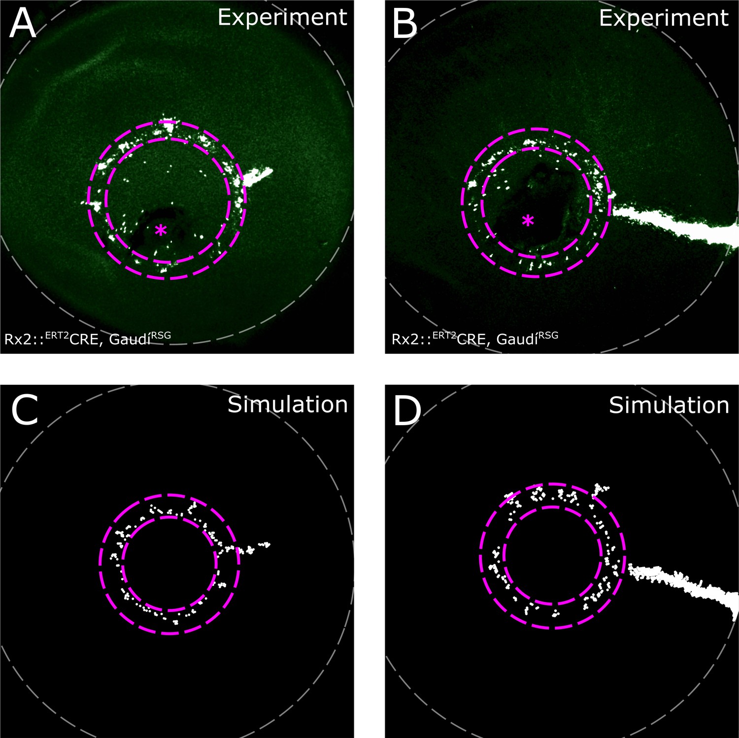
Induction ring in very sparsely labelled samples.
(A–B) Proximal view of NR clones. If label is very sparse, clones occur almost exclusively in the induction ring, with very few or no ArCoS at all, showing that the majority of Rx2-expressing cells form terminated clones. Maximum projection of confocal stack of GFP signal in false colors; rotated to position the optic nerve exit (pink asterisk) ventrally. (C–D) Sparse labelling in simulations. Pink dashed lines encircle induction ring, retinal margin marked by white dashed line.
Figure 5 with 1 supplement
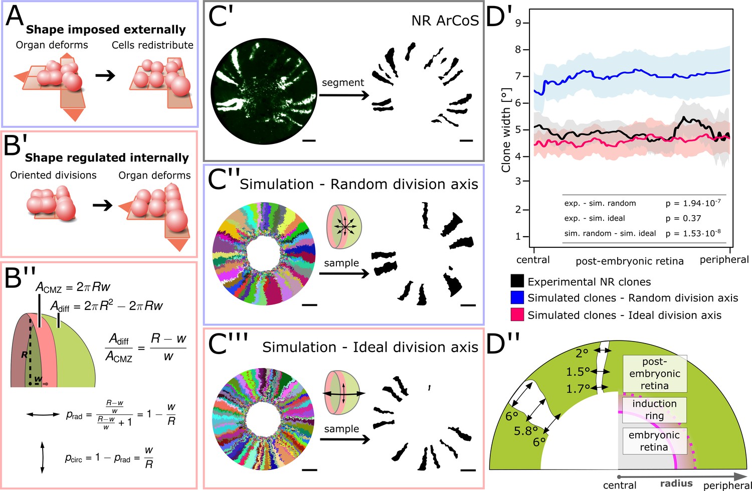
NR stem cells undergo predominant radial divisions as predicted for a shape-giving function.
(A) If organ shape is imposed externally, then cells in the tissue will distribute to fill the available space. Regardless of cell division axes, organ geometry will lead to a directional growth in stripes. (B’) If organ shape is regulated by cell division axes, then oriented divisions are required. (B’’) If the NR regulates shape through cell divisions, then more divisions along the radial axis are needed to maintain hemispherical geometry. (C’–C’’’) Examples of experimental and simulated data. For simulations, the full clone population and a random sample are shown. The initial model label was induced at R = 150 µm to match the experimental induction radius. Scale bars: 200 µm. (D’) Mean clone width (solid lines) and 95% confidence intervals (shaded) plotted along the post-embryonic retinal radius. Experimental data: n = 99 ArCoS across seven retinae. Simulation, random division axis: n = 102 ArCoS from five simulations; ideal division axis: n = 133 ArCoS from five simulations. p values were calculated with Welch two sample t-test. (D’’) Schematic of radial compartments of the NR and measurements of clone width in proximal view. The clone width plotted in D’ corresponds to the angle enclosed by the clone borders at every radial position.
-
Figure 5—source data 1
Mean and 95% confidence interval of clone width.
Figure 5D’) Position along the radius (in µm), mean clone angle (expressed as percent of 360°), and 95% confidence interval for experimental and simulated data.
- https://doi.org/10.7554/eLife.42646.033
Figure 5—figure supplement 1

Average clone width increases with increasing circumferential divisions.
(A’–A’’’) Example simulations where the probability for circumferential divisions was set to a fixed value of 50% (A’), 25% (A’’), and 0% (A’’’). (B) Average clone width along the post-embryonic radius for circumferential division probability ranging from 0% to 50% (one simulation each).
-
Figure 5—figure supplement 1—source data 1
Clone width in simulations with varying circumferential bias.
Figure 5—figure supplement 1B) Position along the radius (in µm) and mean clone angle (expressed as percent of 360°) for simulated data.
Data were obtained for one simulation for each condition.
- https://doi.org/10.7554/eLife.42646.034
Figure 6 with 2 supplements
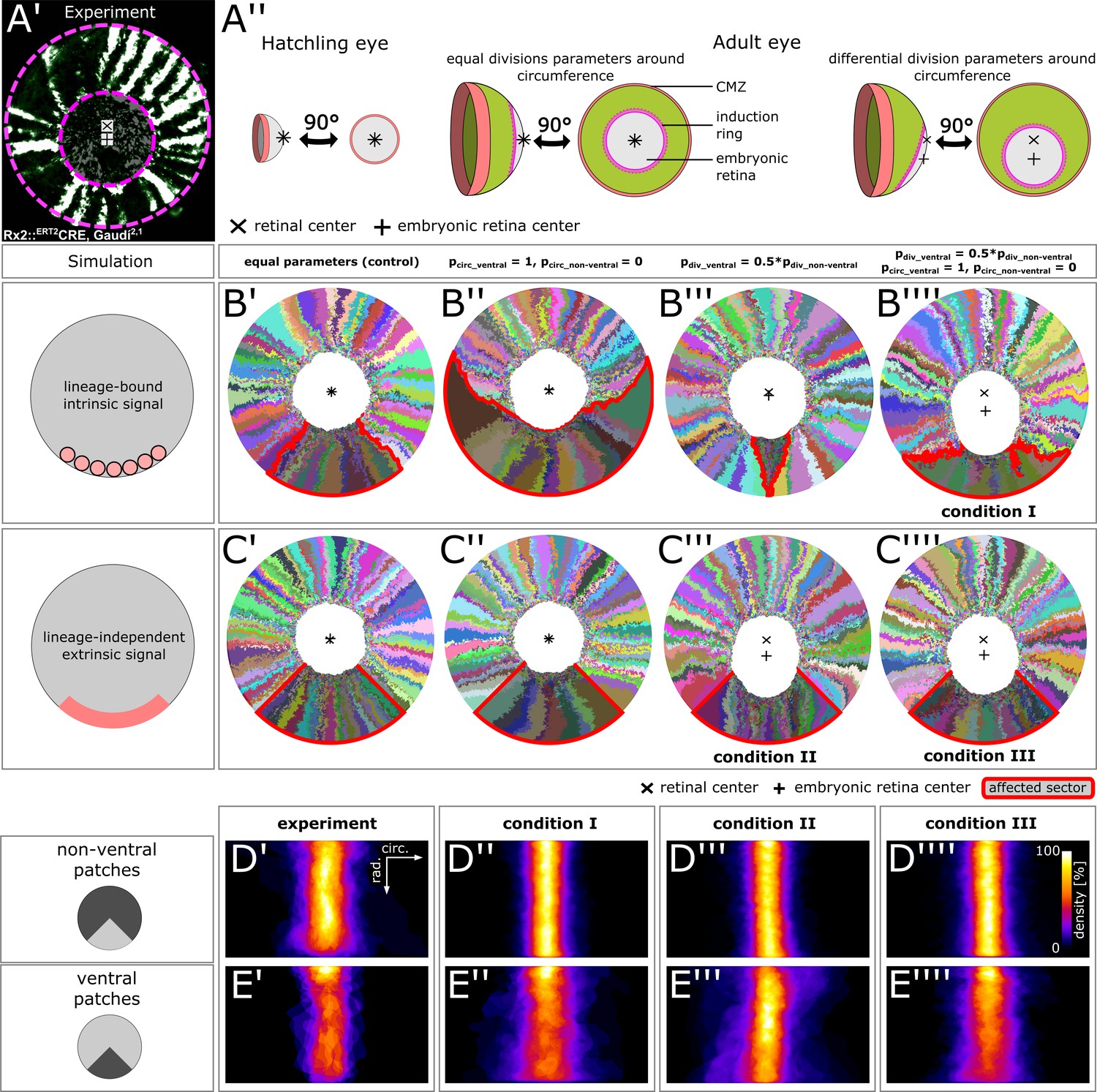
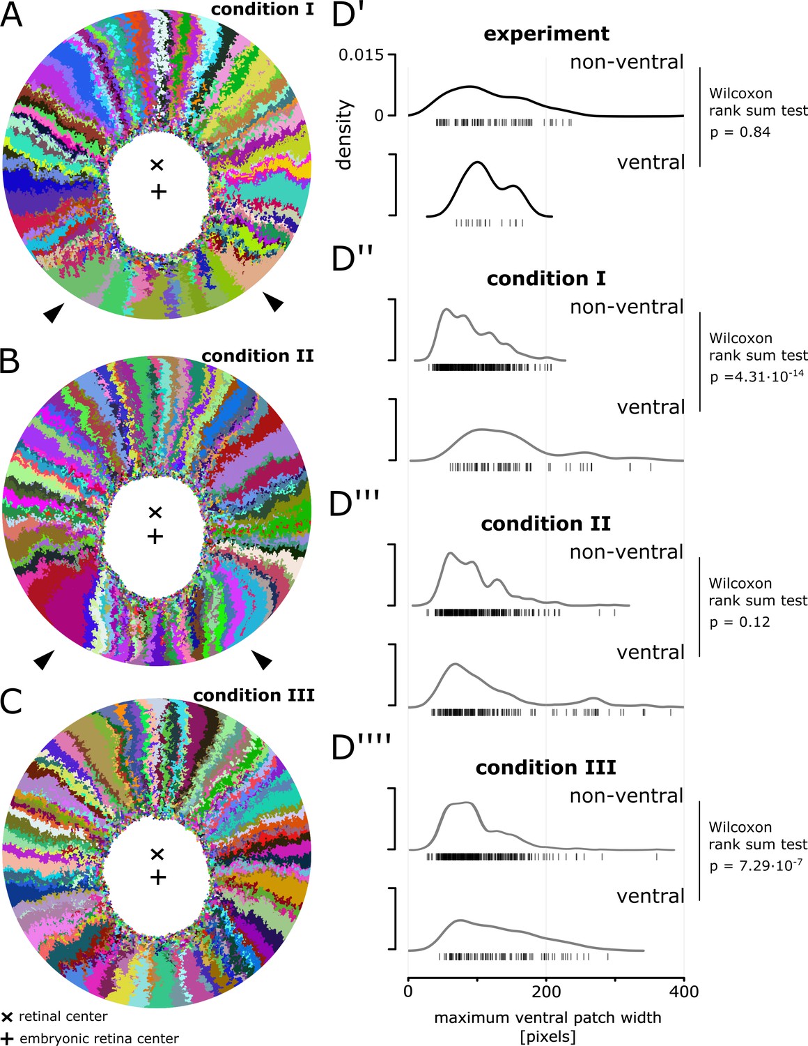
Stem cells in the ventral CMZ have different proliferation parameters.
(A’) Proximal view of NR clones highlighting the discrepancy between retinal center and embryonic retinal center. Depicted sample is the same as in Figure 1D. (A’’) A differential proliferative behavior along the CMZ circumference can explain the shift in position of the embryonic retina. (B’–B’’’’) Simulations where lineages whose embryonic origin is in the ventral sector inherit a signal that leads to different proliferation parameters. A shift occurred when ventral lineages had both lower division probability and higher circumferential divisions. Clones originating in ventral embryonic CMZ are outlined in red. (C’–C’’’’) Simulations where all cells in a ventral 90° sector exhibit different proliferation parameters regardless of lineage relationships. A shift occurred in conditions with slower proliferation as well as slower proliferation combined with circumferential division axis bias. (D’–E’’’’) Patch superposition for experimental data as well as the three simulated conditions that display a ventral shift of the embryonic retina. (D’–D’’’’) Non-ventral patches. (E’–E’’’’) Ventral patches.
-
Figure 6—source data 1
Patch outlines.
Figure 6D’-E’’’’) ‘roi’ format files of aligned individual patch outlines for each condition. Data can be opened in the program ‘ImageJ’.
- https://doi.org/10.7554/eLife.42646.038
Figure 6—figure supplement 1
Magnification of simulations displaying a ventral shift.
(A) Magnification of Figure 6B’’’’. White arrowheads highlight unusually shaped clones with lateral interdigitations. (B) Magnification of Figure 6C’’’. White arrowheads highlight unusually shaped clones that overexpand circumferentially and bend towards the ventral side. (C) Magnification of Figure 6C’’’’. None of the clones display obvious deviations from the average. (D’–D’’’’) Distribution of maximum width of patches that span at least 20% of the radial coordinate.
-
Figure 6—figure supplement 1—source data 1
Patch width distribution.
Figure 6—figure supplement 1D’-D’’’’) Maximum patch width in pixels for each condition. Experimental data are the same as NR data used in Figure 3, but split among ventral and non-ventral patches. For simulated data, the measurements were done on multiple samples from three simulations each.
- https://doi.org/10.7554/eLife.42646.039
Figure 6—figure supplement 2
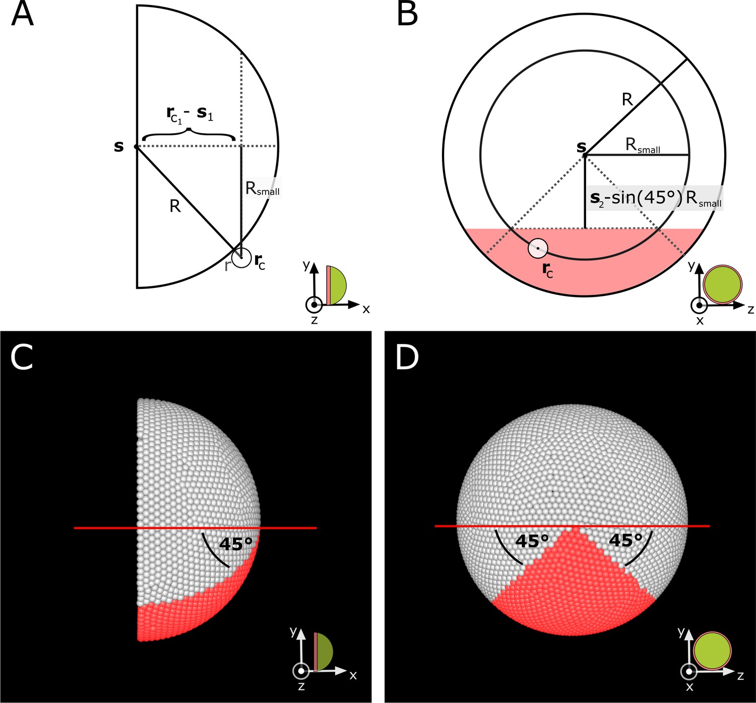
Definition of the ventral sector in the simulation.
(A–B) Schematic side and proximal view showing values used in Appendix 1—equations 16-17 to calculate which cells are located in the ventral sector. For each cell, the corresponding small circle radius is calculated. This cell is assigned to the ventral sector if it lies within the red shaded region in (B). (C–D) Corresponding views in simulation screenshots showing cells in red that satisfy Appendix 1—equations 16-17.
Figure 7

Summary of results and proposed model of CMZ dynamics.
(A) Growth coordination of NR and RPE is achieved by the NR providing instructive stimuli that modulate proliferation of RPE stem cells. As a result of the different growth strategies, variability in cell division timing is elevated in the RPE and lowered in the NR. (B) A base level of variability persists in the NR, such that individual stem cells may differentiate and some multipotent progenitor cells drift to a stem cell fate according to a spatially biased neutral drift model. Thus, stem cells and multipotent progenitor cells have identical proliferative potency. (C) Schematic summary of findings and proposed model, where different NR cell proliferation parameters affect both global and local retinal properties.
Appendix 1—figure 1
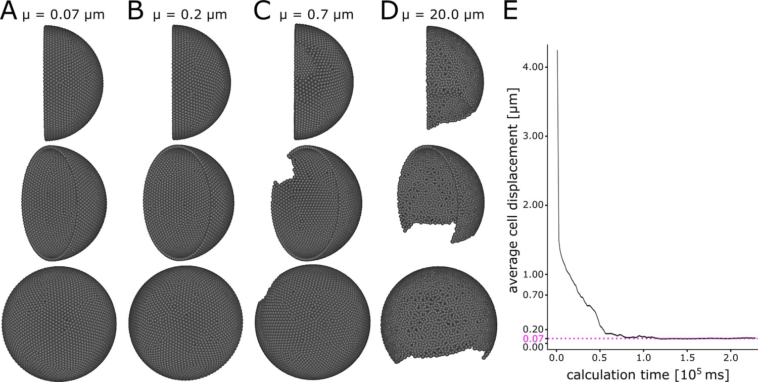
A minimum displacement threshold µ = 0.2 ensures even cell distribution.
Different views of initial condition of the simulation with (A) µ = 0.07 µm, (B) µ = 0.2 µm, (C) µ = 0.7 µm, (D) µ = 20.0 µm. (E) Calculation time plotted against the average cell displacement during initialization of the simulation. The simulation converges to 0.07 µm average displacement (pink dashed line).
Appendix 1—figure 2
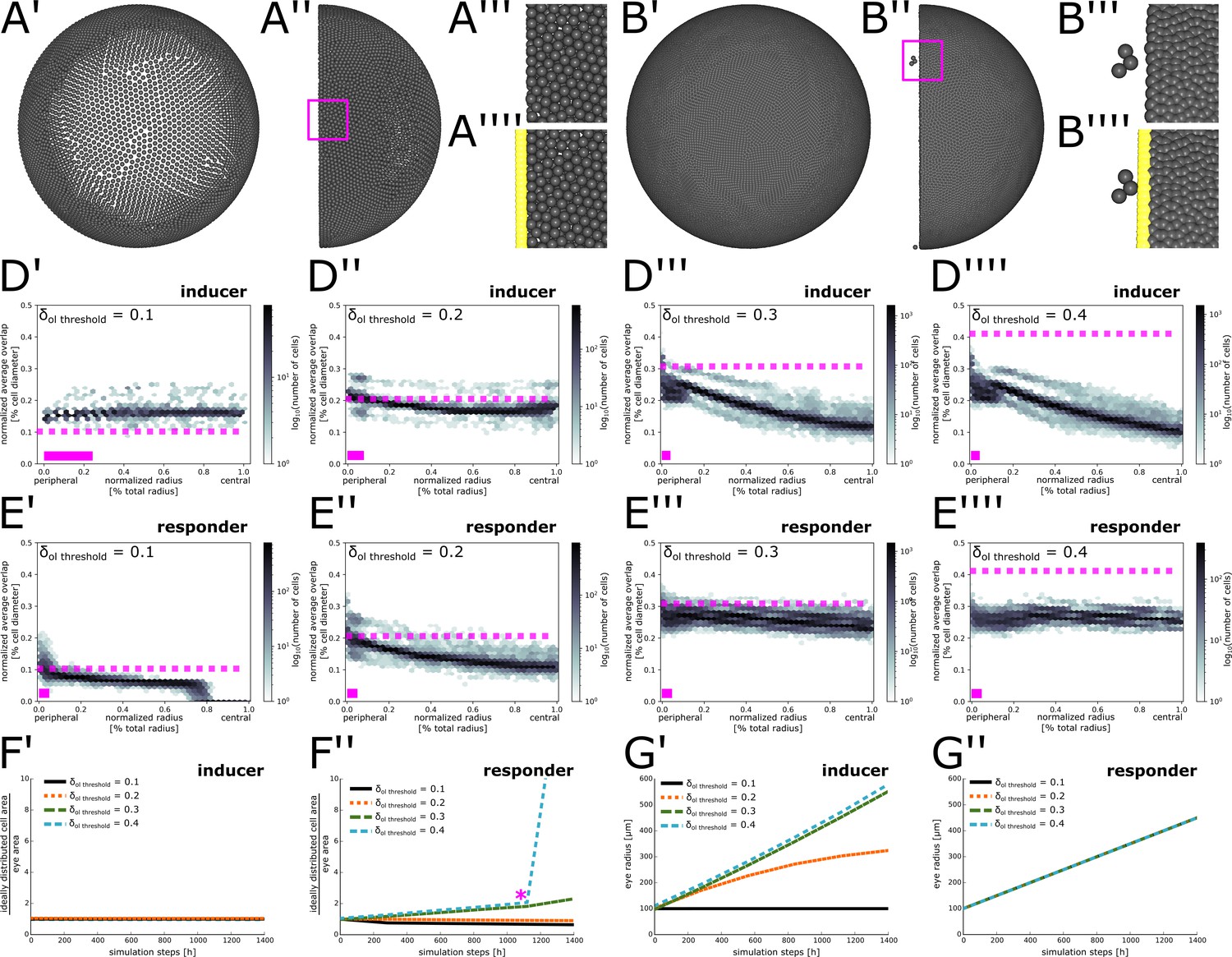
Parameter scan to determine optimal overlap threshold values.
(A’–B’’’’) Different views of representative simulations lacking coupling between eye radius growth and cell proliferation. (A’–A’’) Eye area growth rate exceeds cell proliferation rate, resulting in cell dispersion. (A’’’–A’’’’) Magnification of inset in (A’’) showing peripheral cells without (A’’’) or with (A’’’’) obstacle cells displayed. (B’–B’’) Cell proliferation rate exceeds eye area growth rate, resulting in extremely dense cell packing. (B’’’–B’’’’) Magnification of inset in (B’’) showing peripheral cells without (B’’’) or with (B’’’’) obstacle cells displayed. Three cells have squeezed through the obstacle cell layer. (D’–E’’’’) Normalized average overlap of cells at simulation step 1400 plotted against their position along the normalized radius. Dashed pink line: Value of used for the respective simulation. Solid pink bar: Extent of virtual CMZ. (D–D’’’’) inducer growth mode; (E’–E’’’’) responder growth mode. (F’–F’’) Ratio between total area required by cells and total eye area from simulation step 0 to simulation step 1400 for different values of . (F’) inducer growth mode; (F’’) responder growth mode. Pink asterisk marks approximate time when cells start squeezing through obstacle cell layer. (G’–G’’) Growth of the eye radius from simulation step 0 to simulation step 1400 for different values of . (G’) inducer growth mode; (G’’) responder growth mode.
Appendix 1—figure 3
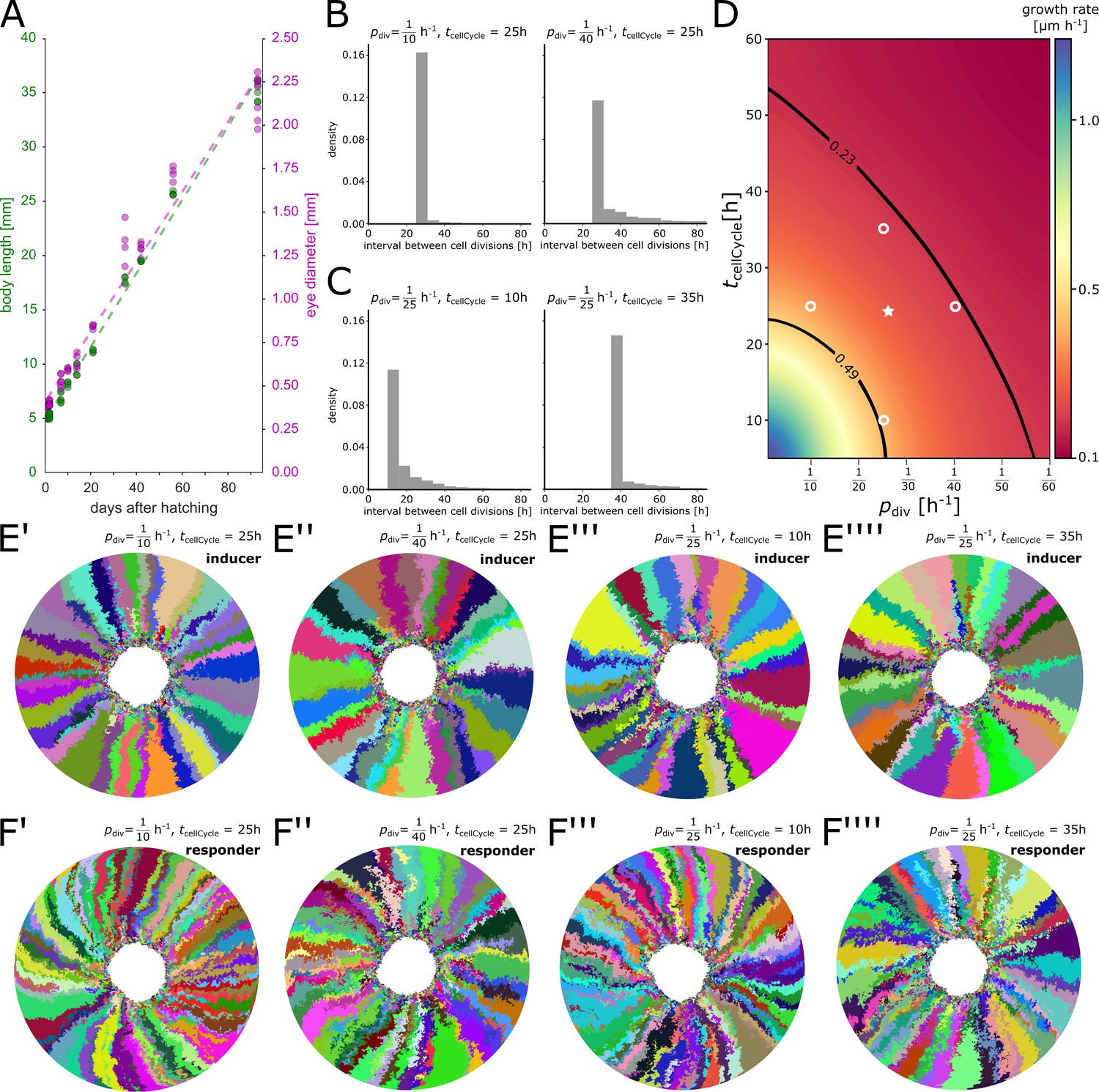
Parameter scan of minimum cell cycle and division probability.
(A) Experimental data. Both body length (green) and eye diameter (magenta) grow approximately linearly over the first 90 days after hatching. (B) Distribution of cell division intervals with fixed and variable . (C) Distribution of cell division intervals with variable and fixed . (D) Eye growth rates in the simulation determined from a parameter scan of and entailing over 150 simulation runs; intermediate values were interpolated. The plausible parameter space estimated from experimental measurements is contoured by black lines. Open white circles represent values for simulations depicted in (B, C, E’–E’’’’, F’–F’’’’). White star represents values used for simulations in the main manuscript. (E’–E’’’’) Representative simulations of the inducer growth mode at different values for and . (F’–F’’’’) Representative simulations of the responder growth mode at different values for and . Throughout the figure is abbreviated as .
Videos
Video 1
The simulated retina is always densely covered by cells.
Simulation of the responder growth mode illustrating clonal lineage formation while the virtual eye grows. When cells divide they briefly flash white.
Video 2
Lateral view of a simulation of the inducer growth mode.
Simulation of the inducer growth mode illustrating clonal lineage formation while the virtual eye grows. When cells divide they briefly flash white.
Video 3
Simulation where 20% of stem cells were labelled in white showing clone fusion and fragmentation.
Cells that were initially differentiated are shown in light gray. When cells divide they briefly flash white.
Video 4
A terminated clone and an ArCoS originating from the peripheral-most stem cell row.
Simulation of the inducer growth mode. Two cells are highlighted in the first simulation step: A purple cell that will give rise to an ArCoS (purple circle), and a green cell that will divide only a few times before its lineage completely exits the niche, forming a terminated clone (green circle). Note how almost all proliferative cells not at the very edge of the hemisphere are pushed out of the proliferative domain and form terminated clones.
Tables
Table 1
List of abbreviations used throughout the main text.
https://doi.org/10.7554/eLife.42646.003| NR | neural retina |
|---|---|
| RPE | retinal pigment epithelium |
| CMZ | ciliary marginal zone |
| Rx2 | retina-specific homeobox gene 2 |
| ArCoS | arched continuous stripes |
| GFP | green fluorescent protein |
| Oca2 | oculo-cutaneous albinism 2 |
| IdU | 5-Iodo-2′-deoxyuridine |
Key resources table
| Reagent type (species) or resource | Designation | Source or reference | Identifiers | Additional information |
|---|---|---|---|---|
| Strain (Oryzias latipes) | Cab | Loosli et al., 2000 | wildtype inbred strain derived fom wild medaka Southern population | |
| Strain (O. latipes) | Rx2::ERT2Cre, GaudíRSG | Centanin et al., 2014; Reinhardt et al., 2015 | ||
| Strain (O. latipes) | Rx2::ERT2Cre, Gaudí2.1 | Centanin et al., 2014; Reinhardt et al., 2015 | ||
| Strain (O. latipes) | GaudíLoxP-OUT | Centanin et al., 2014 | Derived from recombined gametes of Ubi::GaudíRSG. | |
| Sequence- based reagent | short guide RNAs against Oca2 | this paper and Lischik et al., 2019 | target sites: GAAACCCAGGTGGCCATTGC[AGG] and TTGCAGGAATCATTCTGTGT[GGG] | |
| Chemical compound, drug | Tamoxifen | Sigma Aldrich | T5648 | |
| Chemical compound, drug | 5-Iodo-2′-deoxyuridine (IdU) | Sigma Aldrich | I7756 | |
| Chemical compound, drug | Ethyl 3-aminobenzoate methanesulfonate salt (Tricaine) | Sigma Aldrich | A5040 | |
| Antibody | anti-GFP (chicken, polyclonal) | Life Technologies | A10262 | 1:200 |
| Antibody | anti-IdU (mouse, monoclonal) | Becton Dickinson | 347580 | 1:25 |
| Antibody | anti-chicken Alexa Fluor 488 (donkey, polyclonal) | Jackson/Dianova | 703-545-155 | 1:200 |
| Antibody | anti-mouse Alexa 546 (goat, polyclonal) | Invitrogen | A-11030 | 1:400 |
Appendix 1—table 1
Model parameters.
Parameters for the force balance calculation of the biomechanical model are identical to previous work (Sütterlin et al., 2017) and are not listed.
| Description | Parameter | Value | Reference/Explanation |
|---|---|---|---|
| Biomechanical model parameters | |||
| Biomechanical calculation step. | (Sütterlin et al., 2017) | ||
| Seconds per simulation step. | (Sütterlin et al., 2017) | ||
| Optimal overlap for obstacle cells. | Determined by parameter scan to create a tight barrier to cell movement. | ||
| Optimal overlap for retinal cells. | (Sütterlin et al., 2017) | ||
| Initial distance between daughter cells. | (Sütterlin et al., 2017) | ||
| Initial condition parameters | |||
| Initial radius of eye globe. | Estimated from preparations of hatchling eyes. | ||
| Minimal displacement threshold. | Determined by parameter scan to generate even initial cell distribution. | ||
| Simulation parameters | |||
| Retinal cell radius. | Estimated from histological sections. | ||
| Width of the stem cell domain. | Estimated from histological sections. | ||
| Overlap threshold beyond which cell cycle is arrested. | Value for inducer growth mode. Estimated from parameter scan to minimize density-dependent cell cycle arrest. | ||
| Value for responder growth mode. Estimated from parameter scan to maximize density-dependent cell cycle arrest without completely suppressing division. | |||
| Minimal cell cycle length. | Chosen to produce a plausible biological growth rate. | ||
| Probability of cell division. | Chosen to produce a plausible biological growth rate. | ||
| Value for ventral lineages with differential behavior. | |||
| Growth rate of the eye radius (only in responder growth mode). | Chosen as a small value to ensure quasi-static growth within the biologically plausible growth rate range. | ||
Additional files
-
Supplementary file 1
EPISIM Simulator executable model file.
Compiled model file that can be opened in EPISIM Simulator to simulate the model described in this work.
- https://doi.org/10.7554/eLife.42646.041
-
Supplementary file 2
EPISIM Model project archive.
Model project file that can be imported in EPISIM Modeller to visualize the cell behavioral logic implemented in the model described in this work.
- https://doi.org/10.7554/eLife.42646.042
-
Supplementary file 3
Instructions for using supplementary model files.
Step by step instructions on how to open Supplementary file 1 and Supplementary file 2.
- https://doi.org/10.7554/eLife.42646.043
-
Source code 1
EPISIM Simulator implementation of model described in Appendix 1.
Excerpt of the relevant parts of EPISIM Simulator source code. The full source code is available at https://gitlab.com/EPISIM/EPISIM-Simulator (Sütterlin, 2019; copy archived at https://github.com/elifesciences-publications/EPISIM-Simulator).
- https://doi.org/10.7554/eLife.42646.044
-
Transparent reporting form
- https://doi.org/10.7554/eLife.42646.045
Download links
A two-part list of links to download the article, or parts of the article, in various formats.
Downloads (link to download the article as PDF)
Open citations (links to open the citations from this article in various online reference manager services)
Cite this article (links to download the citations from this article in formats compatible with various reference manager tools)
Retinal stem cells modulate proliferative parameters to coordinate post-embryonic morphogenesis in the eye of fish
eLife 8:e42646.
https://doi.org/10.7554/eLife.42646


