Structured illumination microscopy combined with machine learning enables the high throughput analysis and classification of virus structure
- University of Cambridge, United Kingdom
- MedImmune Ltd, United Kingdom
- MedImmune, United Kingdom
Figures
Figure 1 with 2 supplements

Super-resolution microscopy (SRM) for the study of NDV virus structure.
(a) Representative images of purified NDV viruses with different imaging modalities. (b) Representative images of a purified NDV virus population imaged with TIRF-SIM and their corresponding TIRF wide-field image. WF: wide-field TIRF microscopy. Scale bar: 1 µm.
Figure 1—figure supplement 1
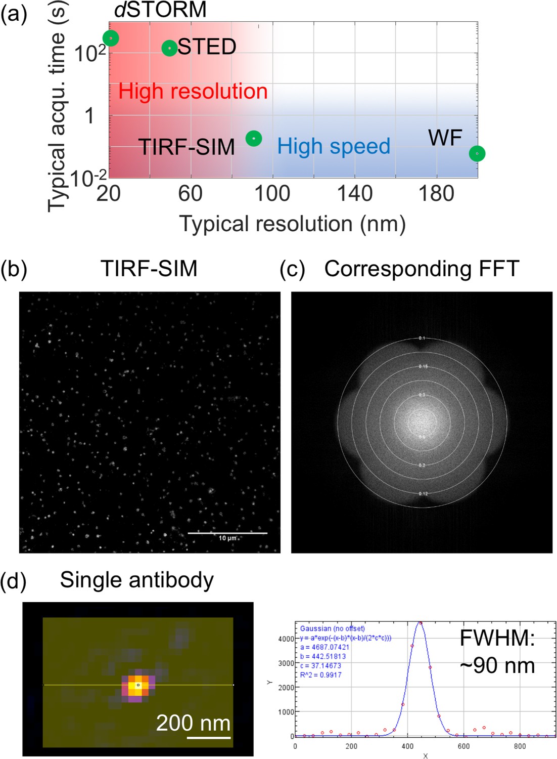
Resolution in SRM.
(a) Typical spatial resolution and acquisition times for the imaging of NDV structures highlighting the trade-off between speed and resolution (b) Representative TIRF-SIM image obtained from purified B Victoria LAIV and its corresponding Fourier transform (c). The Fourier transform highlights the resolution ~90 nm. The plot was obtained using the SIMcheck plugin (Ball et al., 2015). (d) Image and cross section of a single secondary antibody labelled with DyLight 488, showing a FWHM of ~90 nm. FFT: Fast Fourier transform.
Figure 1—figure supplement 2
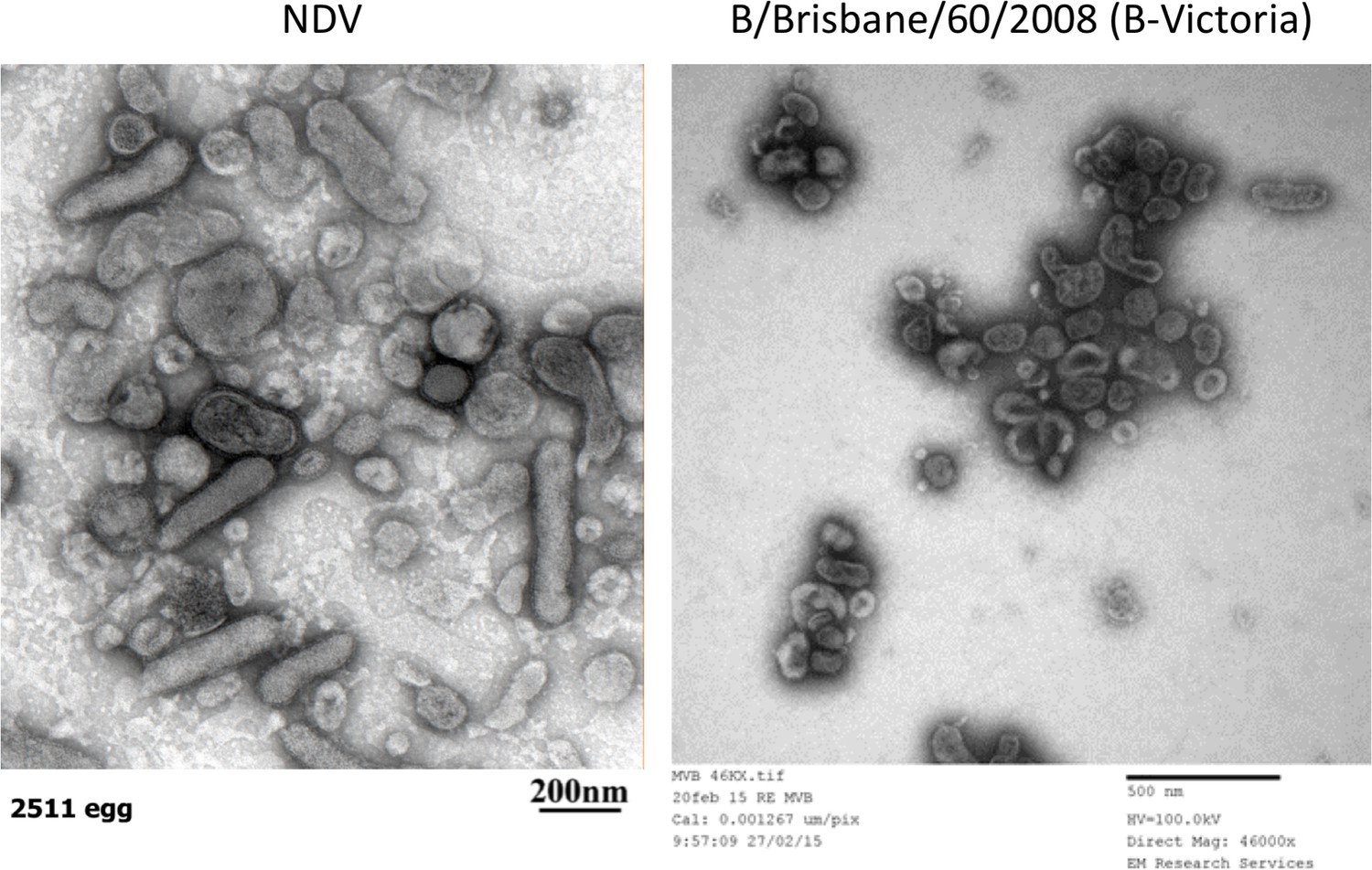
Electron micrographs of NDV and B-Victoria viruses.
These images were obtained from a Philips CM 100 Compustage (FEI) TEM and negative staining.
Figure 2 with 1 supplement
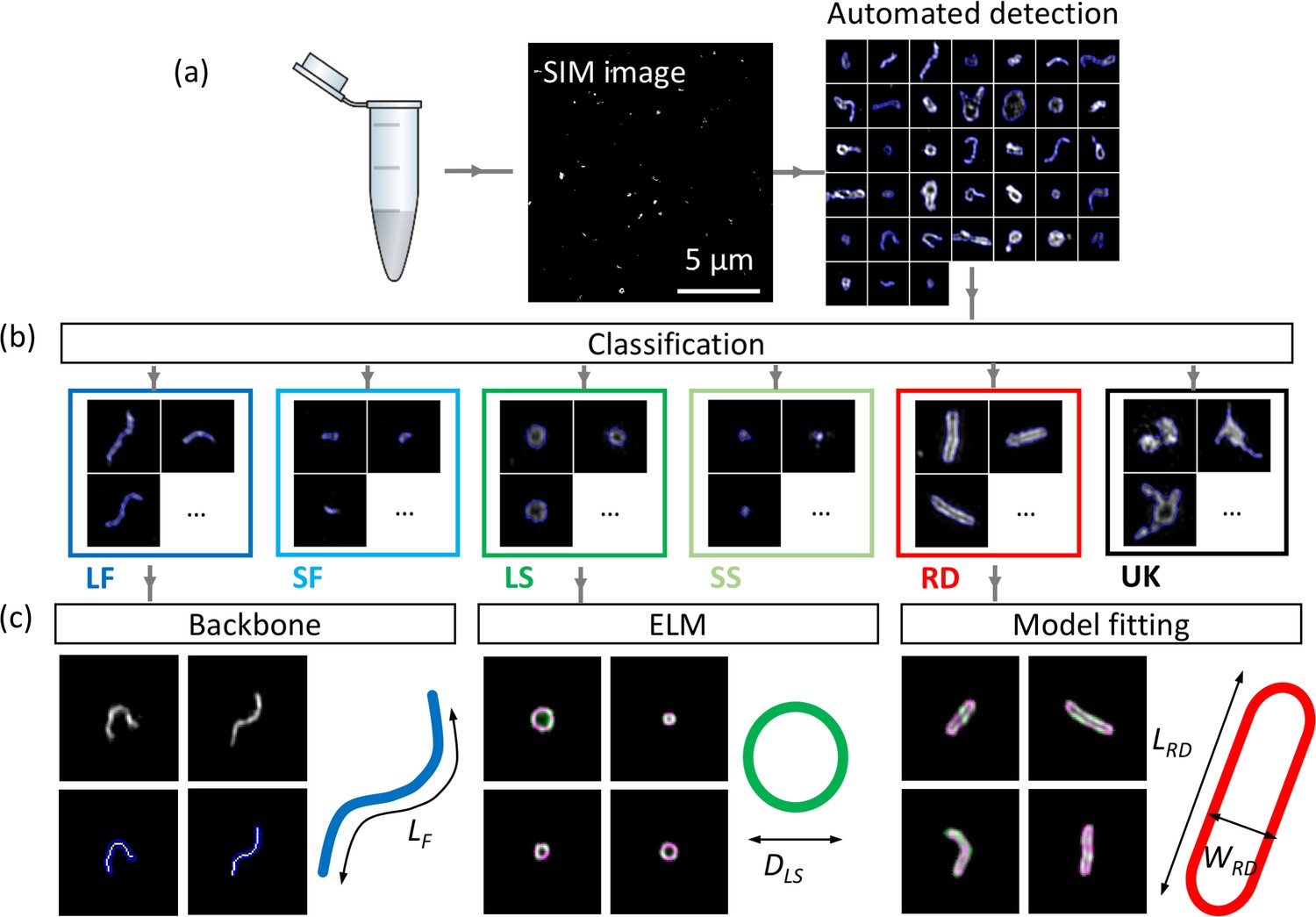
Workflow of automated detection, classification and analysis of NDV viral particles.
SIM image (a) and segmented particles (b). The classified single-virus images (b) can be further analysed with a set of class-specific tools (c). For the backbone analysis the mask and backbone are showed in blue and white respectively. For the model-fitting approach (spherical and rod-like), the data and model are showed in green and magenta respectively. LF: long filamentous, SF: short filamentous, LS: large spherical, SS: small spherical, RD: rod-shape, UK: unknown. LF, DLS, LRD and WRD represent the length of the filamentous particles, the diameter of the large spherical, the length of the rod-shaped particles and the width of the rod-shaped particles respectively. Images of individual particles cover a field of view of 1.6 × 1.6 µm.
Figure 2—figure supplement 1
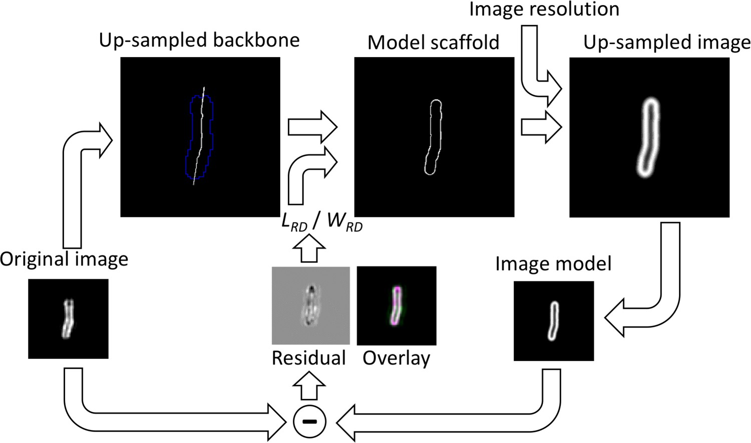
Image model for the analysis of the rod-shaped particles.
The original image is segmented and thinned to obtain the backbone of the particle. The backbone is up-sampled and interpolated outside the particle. It is then used to compute the model scaffold. For this, each end of the backbone is independently grown or reduced to adjust its length, hence LRD = Ltot – L1 – L2, where Ltot is the maximum length of the extended backbone, and L1 and L2 are the adjusted distances by which the backbone length is adjusted on each end respectively. Then, the image is dilated by a disk-shaped kernel of radius equal to half WRD. The outline of this image gives the model scaffold. The scaffold is then convolved with a Gaussian kernel representing the effect of image resolution (here 90 nm) and the image is down-sampled again to the original image size. The optimal LRD and WRD are those that minimize the difference image and the χ (Müller and Heilemann, 2013).
Figure 3 with 1 supplement
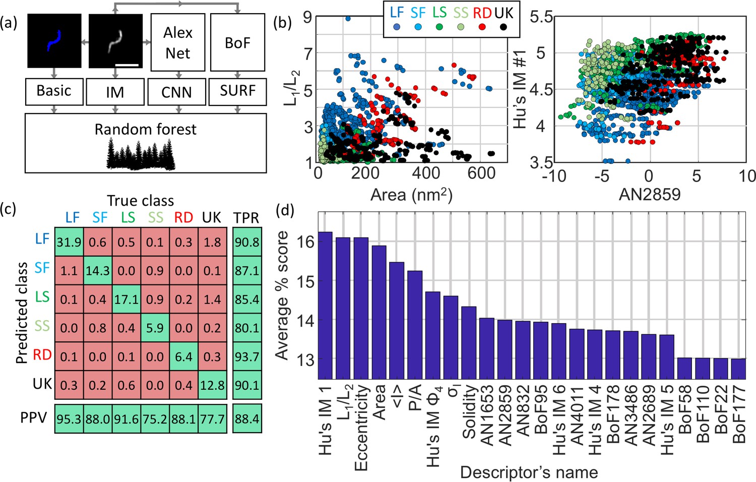
Machine learning-based classification.
(a) Building the list of predictors from basic features, image moments, convolutional neural network (CNN) features and SURF bag of features (BoF). (b) Example of 2D scatter plots of pairs of predictors showing how some predictors allow identification of class clusters. (c) Confusion matrix obtained from the random forest showing the high true positive rate (TPR) and positive predictive values (PPV) of the classification. All numbers shown here are in percentage. (d) Scoring of the predictors sorted in descending order. IM: image moment. AN: AlexNet feature. BoF: SURF features. L1/L2: ratio of long axis over short axis. <I> : average intensity. P/A: perimeter to area ratio. σI: standard deviation of intensity. LF: long filamentous, SF: short filamentous, LS: large spherical, SS: small spherical, RD: rod-shape, UK: unknown.
Figure 3—figure supplement 1

Flowchart describing the machine learning pipeline used here for image classification.
A strong emphasis should be put on the choice of predictors and the quality of the manual annotation (training dataset) prior to classification, as this will largely determine the quality of the classification.
Figure 4 with 1 supplement
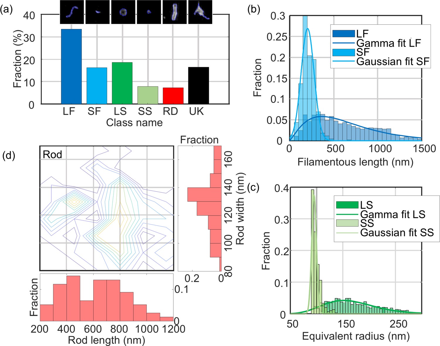
Quantitative analysis of NDV.
The distribution of structural parameters for all classes was obtained from a total of ~6500 virus particles. LF: long filamentous, SF: short filamentous, LS: large spherical, SS: small spherical, RD: rod-shape, UK: unknown. Images of individual particles cover a field of view of 1.6 × 1.6 µm.
-
Figure 4—source data 1
Source data for Figure 4.
- https://doi.org/10.7554/eLife.40183.013
Figure 4—figure supplement 1
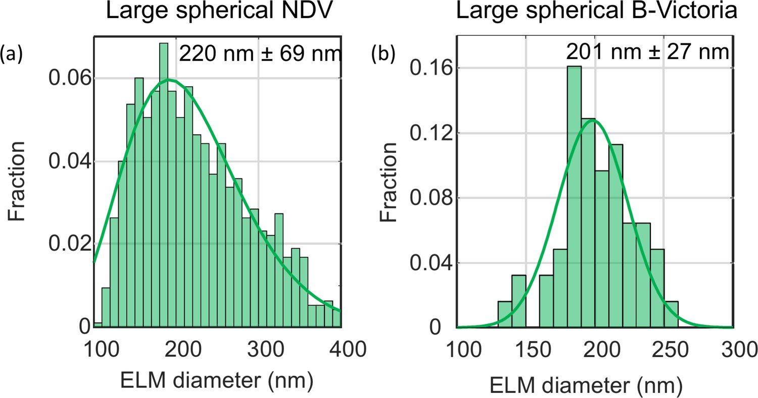
ELM analysis of the large spherical NDV.
(a) and B-Victoria LAIV (b) viruses. The distribution of diameters were fitted to a Gamma and Gaussian distributions respectively. The mean diameters and standard deviations of the data are shown.
Figure 5 with 1 supplement
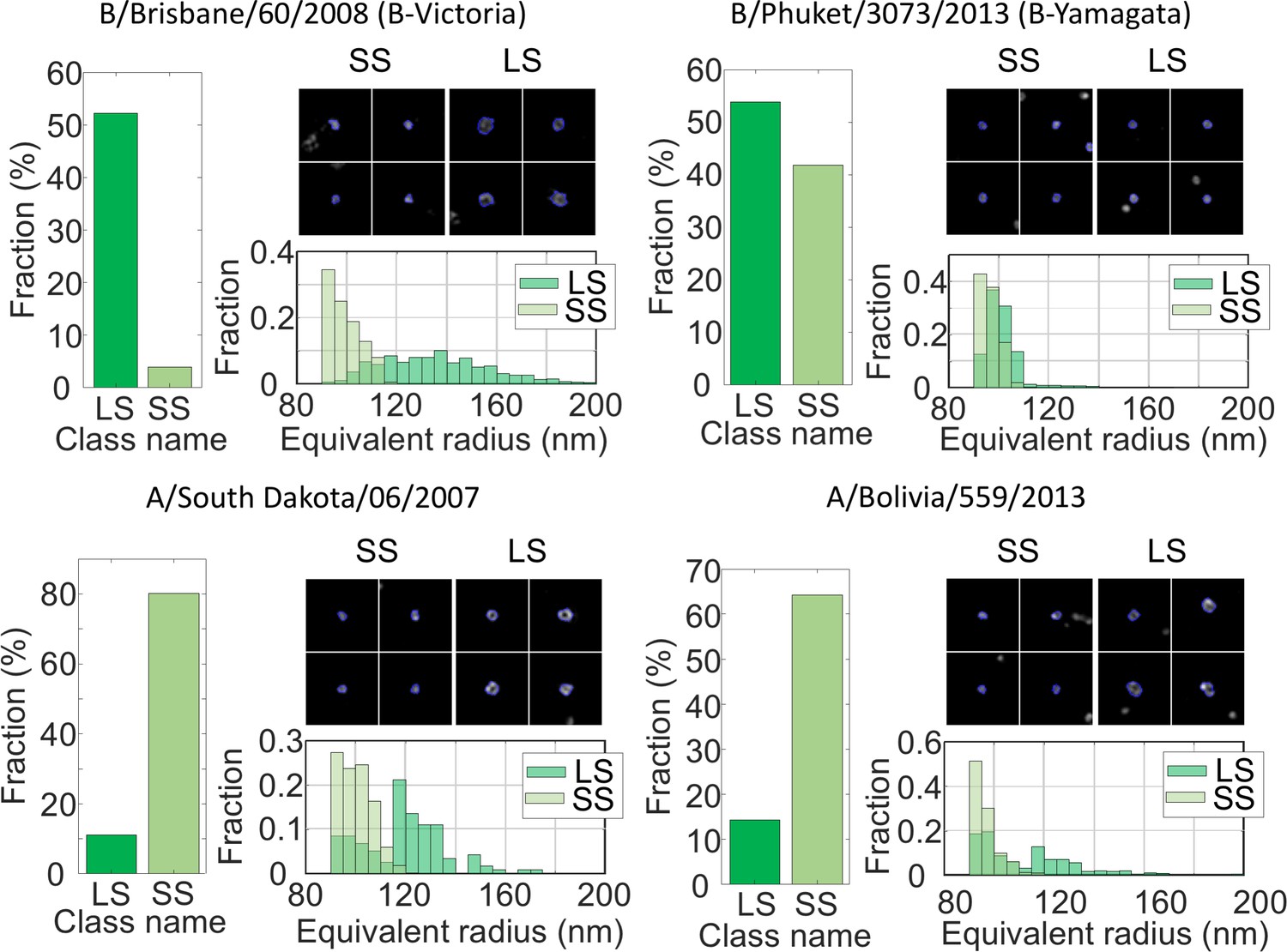
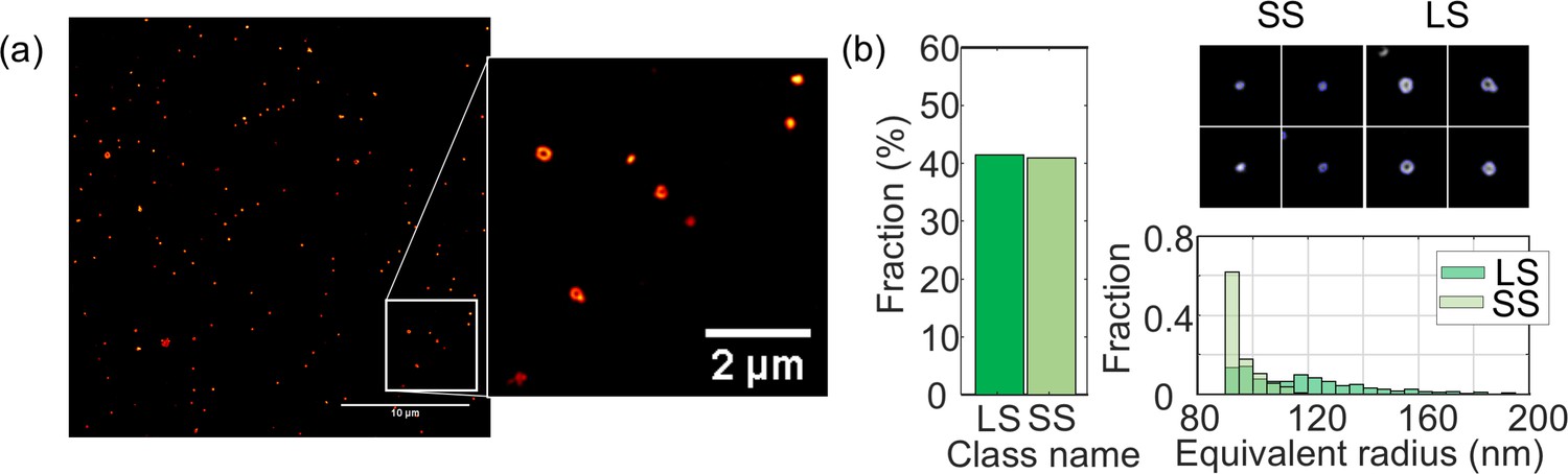
MiLeSIM approach applied to Live Attenuated Influenza Virus (LAIV).
2 types of B and A viruses were analysed here. The population was dominated by small and large spherical particles. The distributions of equivalent radius are shown here for both the large and small spherical for direct comparisons. The number of particles analysed were N = 3,821, 4704, 1062 and 1756 for B/Brisbane/60/2008 (B-Victoria), B/Phuket/3073/2013 (B-Yamagata), A/South Dakota/06/2007 and A/Bolivia/559/2013 respectively. Images of individual particles cover a field of view of 1.6 × 1.6 µm.
-
Figure 5—source data 1
Source data for Figure 5.
- https://doi.org/10.7554/eLife.40183.016
Figure 5—figure supplement 1
Structural analysis of B-Victoria LAIV obtained from pool harvested fluid (PHF).
(a) TIRF-SIM images. The images acquired here using PHF show an identical image quality as with highly purified samples. (b) Structural analysis of N = 1295 virus particles. Images of individual particles cover a field of view of 1.6 × 1.6 µm.
Tables
Table 1
Comparison of the key performance parameters of TIRF-SIM (proposed method) and EM in the context of high throughput imaging of virus structure.
The resolution and acquisition time of EM were quoted for a standard TEM imaging (Philips CM 100 Compustage (FEI) Transmission Electron Microscope with an AMT CCD camera). *for a comparable field-of-view.
| Tirf-sim | EM | |
|---|---|---|
| Contrast | Fluorescence | Electron scattering |
| Molecular specificity | Very high | Medium to low |
| Spatial resolution achievable | ~90 nm | ~1 Å |
| Acquisition time/1000 virus particles* | 2 s | 2 s |
| Typical field of view size | 30 µm x 30 µm | 500 nm x 500 nm |
| Sample preparation complexity | Low | Low to Medium |
| Compatibility with aqueous buffers | High | Low |
| Compatibility with non-purified samples | High | Low |
| Signal to noise ratio achievable | Very high | Medium |
| Sample preparation time | Low (2–3 hr) | Low to High |
| Expertise required for imaging | Medium | Medium |
| Cost | Low (£100 k) | Medium (£250 k) |
Table 2
Estimation of the time necessary to perform individual steps involved in MiLeSIM.
Sample preparation was estimated based on standard immuno-labelling protocols. The computational times were assessed on an analysis machine with an i7 processor at 3.5 GHz and 64 GB of RAM.
| Step | Description | Time |
|---|---|---|
| Sample preparation | Plating, permeabilising and immune-labelling of virus particles | 2–3 hr |
| Instrument set-up | Quality check of set-up alignment, calibration and sample mounting | 30 min |
| Imaging | Image acquisition, stage movement and refocus for ~ 50,000 particles (50 fields-of-view) | 30 min |
| SIM reconstruction | SR reconstruction of 50 fields-of-view | <30 min |
| Classification on unknown data | Extraction of predictors and classification (for 50 fields-of view) | 1h |
| Structural analysis | Extraction of structural parameters for each classes (for 50 fields-of view) | 1h |
| Data curation for training dataset | Generating manually labelled particle dataset (performed only once) for ~ 500 particles | 2h |
| Generating classification model | Data augmentation, extraction of predictors, training of the model, cross-validation on ~ 500 particles (performed only once) | 5–6 hr |
Additional files
-
Transparent reporting form
- https://doi.org/10.7554/eLife.40183.018
Download links
A two-part list of links to download the article, or parts of the article, in various formats.
Downloads (link to download the article as PDF)
Open citations (links to open the citations from this article in various online reference manager services)
Cite this article (links to download the citations from this article in formats compatible with various reference manager tools)
Structured illumination microscopy combined with machine learning enables the high throughput analysis and classification of virus structure
eLife 7:e40183.
https://doi.org/10.7554/eLife.40183


