Phenotypic diversity and temporal variability in a bacterial signaling network revealed by single-cell FRET
- AMOLF Institute, The Netherlands
- Yale University, United States
Figures
Figure 1 with 3 supplements
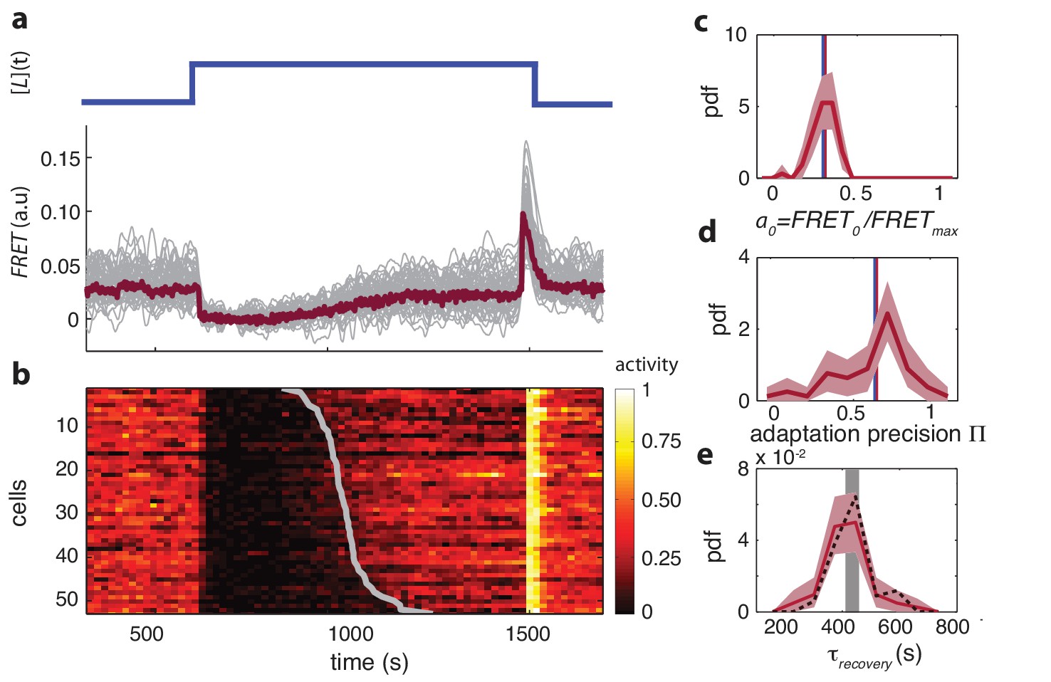
Single-cell FRET over extended times reveals cell-to-cell variability in signaling response.
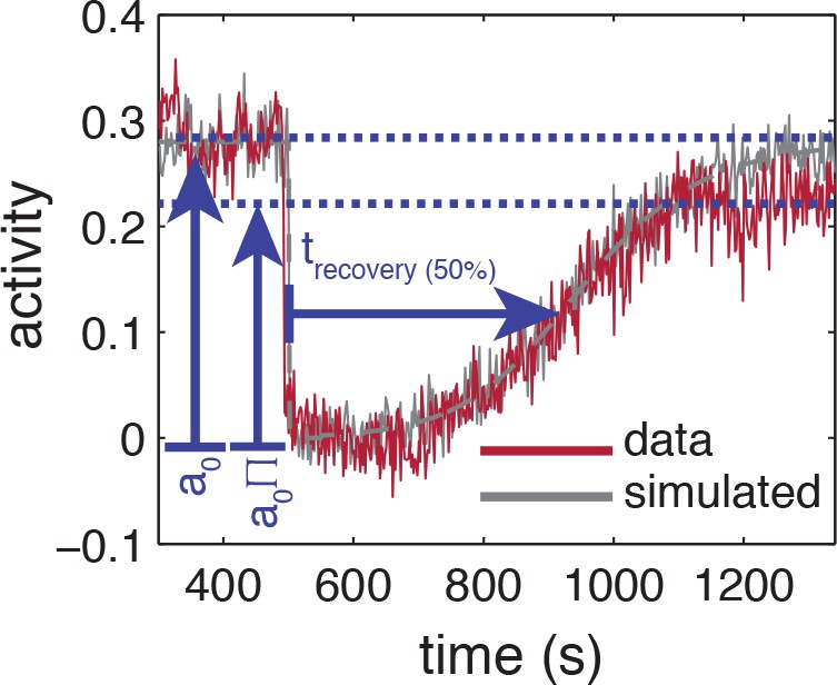
(a) Step-response experiment on wildtype cells (CheRB+; VS115). (Top) The ligand time series indicates the applied temporal protocol for addition and removal of 500 μM MeAsp. (Bottom) FRET response of 54 cells (grey) with the ensemble-averaged time series (dark red) overlaid from a representative single experiment. Single-cell time series were lowpass filtered with a 14 s moving-average filter. (b) Heatmap representation of the normalized FRET response time series, with each row representing a single cell, and successive columns representing the 10 s time bins in which the color-indicated activity was computed from the FRET time series. Activity was computed by normalizing FRET to the total response amplitude (Max-Min for each time series). Rows are sorted by the corresponding cell’s recovery time (grey curve), defined as the time at which the activity recovered to 50% of the activity level after adaptation (see panel e). Single-cell FRET assay schematic and image processing pipeline are shown in Figure 1—figure supplement 1. (c) Steady-state activity of the cells shown in panels (a–b). Also shown are the mean steady-state activity (red vertical line) and the steady-state activity of the population averaged time series (blue vertical line). (d) Adaptation precision obtained from the FRET data. An adaptation precision of 1 denotes perfect adaptation. Also shown are the mean precision (red vertical line) and the precision of the population averaged time series (blue vertical line). The mean and std of the distribution is 0.79 0.32. All colored shaded areas represent 95% confidence intervals obtained through bootstrap resampling. (e) Recovery time of cells defined as time to reach 50% of the post-adaptational activity level (red, 54 cells) or 50% of pre-stimulus activity (black dashed, 44 cells with precision >0.5) and simulated effect of experimental noise for a population with identical recovery times (grey). The latter was obtained from a simulated data set in which 55 time series were generated as described in Figure 1—figure supplement 3. The width of the bar is defined by the mean ± std of the simulated distribution. The mean ± std of the distributions for the experimental and simulated data sets are respectively 416 ± 83 and 420 ± 35 s.
-
Figure 1—source data 1
Source data (.mat) file containing FRET data and analysis.
- https://doi.org/10.7554/eLife.27455.007
Figure 1—figure supplement 1

Single-cell FRET assay schematic and workflow.
(a) Schematic of CheY-CheZ FRET assay. In absence of ligand stimuli, receptors are activating CheA. When active, CheA phosphorylates CheY, increasing interaction between CheY and phosphatase CheZ and thereby increasing FRET through the labeled fluorophores. Ligand-receptor binding shuts down the kinase, which ceases phosphate transfer and FRET levels decrease. (b) False-color images of donor (CheZ-YFP) and acceptor (CheY-mRFP1) fluorescence, channels projected on the same EM-CCD camera chip. (c) Example time series fluorescence from a single cell (CheRB-,VS149/pVS149/52). In grey raw data is shown, with a fit to a single exponential function with offset overlaid for donor (top, green) and acceptor channel (middle, red). From the corrected fluorescence intensities the ratio RFP/YFP is calculated (bottom). (d) FRET protein fusions approach wildtype chemotaxis performance on soft agar. Cells without endogenous CheY and CheZ (ΔYZ, VS104) carrying FRET plasmids expressing CheZ-YFP and CheY-mRFP1 pSJAB12, 106 and 109 (see Table 4) induced with 100 μM IPTG and one empty pBAD33 plasmid exhibit proper chemotaxis performance on soft agar with the double ring expansion visible. Performance of pSJAB106 approaches the WT performance (RP437, two empty plasmids).
Figure 1—figure supplement 2
The observed diversity in signaling parameters can not be explained by variation in experimental parameters and is reproducible.
(a) Histogram of fluorescence intensities intensities of the donor at the start of a FRET experiment as measured (purple, CV=0.38) and corrected for inhomogeneous illumination (grey, CV=0.33). (b) Scatter plots of donor intensity versus adaptation timescale (top panel), adaptation precision (middle panel) and steady-state activity (bottom panel). For each scatter, the data points (red) are shown together with the intensities corrected for inhomogeneous illumination (grey). Above each plot the Pearson correlation coefficient is shown with 95 % confidence interval obtained from bootstrap resampling. (c) Scatter plot of euclidean distance (in pixels) of each cell to sample position with highest illumination intensity versus the donor intensity. Illumination correction changes a negative dependence of cellular intensity to distance (ρ=-0.44±0.15) to insignificant dependence (ρ=-0.19±0.21). (d) Scatter plots of euclidean distance (in pixels) of each cell to sample position with highest illumination intensity versus adaptation timescale (top panel), adaptation precision (middle panel) and steady-state activity (bottom panel). Above each plot the correlation coefficient is shown with 95 % confidence interval obtained by bootstrap resampling. (e) Histogram of the intact fraction (1-decay) of donor fluorescence intensity at the end of the FRET experiment. (f) Illumination profile measured by illuminating a ~100 μm thick sample with fluorescein. (g) Reproducibility of signaling parameters. Shown are the experiment used in panels (a) to (e) and the main figure (54 cells, purple) as well as an independent repeat (71 cells, green) for the adaptation timescale (top panel), adaptation precision (middle panel) and steady-state activity (bottom panel). Coefficients of variation are shown with corresponding colors in each panel.
Figure 1—figure supplement 3

Influence of experimental noise on estimating recovery times.
Simulated time series are calculated by integrating the linearized MWC model with adaptation kinetics (Tu et al., 2008) with parameters chosen to closely approximate the population averaged response (grey-dashed line). To the simulated time series of each cell, gaussian white noise , 55 cells) is added to approximate the noise level of the experiment. Also shown are the baseline and recovery levels (blue dashed lines) of the experimental population.
Figure 2 with 3 supplements
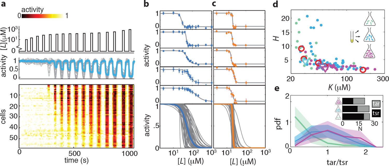
Ligand dose-response parameters vary strongly across cells in an isogenic population, even in the absence of adaptation, and depend on receptor-complex composition.
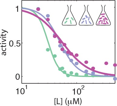
(a) Single-cell dose-response experiment on adaptation deficient (CheRB-; TSS58) cells with a wildtype complement of receptors. (Top) Temporal protocol of stimulation by the attractant L-serine. (Middle) The ensemble-averaged FRET response of the population (blue) and single cells (gray) in signaling activity of 59 cells from a single experiment, normalized to the full-scale FRET response amplitude. (Bottom) Heatmap representation of the single-cell FRET timeseries, with the rows sorted by the sensitivity of the corresponding cell obtained from Hill-curve fits. (b) Ensemble of Hill-curve fits (gray) to single-cell dose-response data from a single experiment on CheRB- cells with a wildtype complement of receptors (TSS58). Fits for five example cells from the ensemble are shown above together with data points (error bars: 2 s.e.m. over 19 frames). The blue curve overlaid on the ensemble was obtained by applying the same analysis to the population-averaged time series shown in panel (a), yielding fit values =50 ± 3 μM and =2.7 ± 0.5. (c) As in panel (b), but with CheRB- cells expressing only the serine receptor Tsr (UU2567/pPA114). The orange curve was obtained from fits to the population average, yielding =20.0 ± 0.3 μM and =22 ± 8. (d) Cells from a single overnight culture were inoculated into three flasks harvested at different times during batch-culture growth to sample the state of the population at three points along the growth curve: at OD = 0.31 (green), 0.45 (blue) and 0.59 (purple). Fits to the population-averaged time series are shown in Figure 2—figure supplement 2. Shown are Hill-curve sensitivity and cooperativity obtained from fits to the single-cell dose-response data, at different harvesting OD’s (filled dots) together with the fit values for the population-averaged dose-response data (triangles). Also shown are population-FRET results from (Sourjik and Berg, 2004) in which the average Tar and Tsr levels were tuned using inducible promotors (red circles). Shown are 25 out of 28 cells harvested at OD = 0.31, 59 out of 64 cells at OD = 0.45, 34 out of 40 cells at OD = 0.59. The excluded cells had fits with a mean squared error higher then 0.05. The influence of experimental noise on the fit parameters is shown in Figure 2—figure supplement 3. (e) Histograms of Tar/Tsr ratio obtained by fitting the multi-species MWC model from (Mello and Tu, 2005) to single-cell FRET time series. The mean Tar/Tsr ratios (low to high OD) are 0.4, 0.9, and 1.2 with coefficients of variance of respectively 1.1, 0.5, and 0.4. Inset: average cluster size (MWC-model parameter N) of Tar (grey) and Tsr (black) at different harvesting OD’s obtained from the fit results in panel d.
-
Figure 2—source data 1
Source data (.mat) file containing FRET data and analysis.
- https://doi.org/10.7554/eLife.27455.012
Figure 2—figure supplement 1
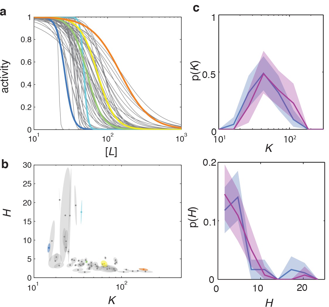
Dose response curve parameters uncertainty estimation and reproducibility.
(a) Fitted dose response curves for five representative cells are highlighted in color, within the ensemble for a population of 59 cells from a single experiment (same data as Figure 2). (b) and parameter-fit uncertainty basins, with long and short axes obtained from eigendecomposition of the covariance matrix for each fit, with the highlighted cells corresponding to the same example cells as in panel (a). (c) Day-to-day variability in dose-response phenotype distributions. Distribution of parameter (top) and (bottom) from a single FRET experiment performed on different days. Together with the data from panels a-b (blue) an additional experiment is shown with 44 out of 45 cells. Shaded areas represent 95 % confidence intervals obtained by bootstrap resampling.
Figure 2—figure supplement 2
Dose response curves from population averaged time series at different harvesting OD's.
Dose response curves from population-averaged time series for CheRB- cells with a WT receptor complement (TSS58) harvested at OD = 0.31 (green), OD = 0.45 (blue) and OD = 0.59 (purple).
The fit-value pairs are respectively , , and .
Figure 2—figure supplement 3

Influence of experimental noise on fit parameters and , for Hill curve fits to single-cell dose-response data.
Colored points and lines are fitted parameter-value pairs and marginal histograms, respectively, for measured dose-response data. Gray points and lines are the same for simulated data in which gaussian noise is added to the population-level dose response curve (with and obtained from fitting the population-averaged time series). The gaussian noise intensity in the simulation is chosen to match the average mean-squared error [MSE] of the dose response curve fits. Experimental data with a MSE exceeding a determined threshold (0.05) are removed from the analysis. (a) Cells with WT receptor complement (TSS58) harvested at OD = 0.45 (5 cells excluded by MSE) (b) TSS58 cells harvested at OD = 0.59 (6 cells excluded by MSE) (c) TSS58 cells harvested at OD = 0.31 (3 cells excluded by MSE). (d) CheRB-Tsr+ (UU2567/pPA114) cells harvested at OD = 0.45. (11 cells excluded by MSE). All shaded areas indicate 95 % confidence intervals obtained by bootstrap resampling.
Figure 3 with 5 supplements
CheB phosphorylation feedback attenuates variability in steady-state kinase activity.
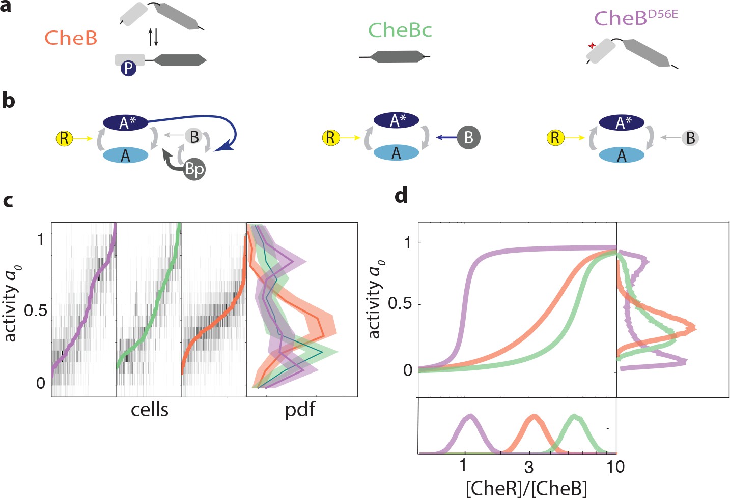
(a) Schematic depiction of CheB activation by phosphorylation. (Top) CheB consists of two domains connected by a flexible linker. The aspartate at residue 56 within the N-terminal receiver domain can be phosphorylated. (Middle) CheBc lacks the receiver domain with the phosphorylation site. (Bottom) CheB-D56E carries a point mutation at the phosphorylation site. (b) Effective network topology of cells expressing WT CheB (top), CheBc (middle) and CheB-D56E (bottom). All three topologies are capable of precise adaptation due to activity-dependent feedback (Barkai and Leibler, 1997). (c) Heatmap representation of histograms of the activity about the unstimulated steady-state of single cells, from FRET experiments of the type shown in Figure 3—figure supplement 1. Each column represents a single cell, sorted by the steady-state activity (colored curves) for each CheB mutant expressed in a cheB background (VS124, colors as in panel (a)). (right) Normalized histograms (probability density function, pdf) of for each CheB mutant. Histograms contain results for cells with a signal-to-noise ratio greater than one from at least three independent FRET experiments, corresponding to 231 out of 280 cells (WT), 169 out of 210 cells (CheBc) and 156 out of 246 cells (D56E). Shaded regions represent bootstrapped 95% confidence intervals. We verified that the bimodality was not due to clipping from FRET-pair saturation, by mapping the dependence of FRET on donor/acceptor expression (Figure 3—figure supplement 2). (d) A simple kinetic model of the chemotaxis network illustrates the crucial role of CheB phosphorylation feedback in circumventing detrimental bimodality in . Due to sublinear enzyme kinetics in the adaptation system, the transfer function =ƒ([R]/[B]) mapping the P([R]/[B]) expression ratio to steady-state network output can be highly nonlinear (main panel). The shape of this transfer function determines the distribution P of steady-state activity (right panel) by transforming the distribution P([R]/[B]) of adaptation-enzyme expression ratios (bottom panel). Three variations of the model are shown, corresponding to WT (orange, with phosphorylation feedback), CheB (purple, no phosphorylation feedback and low catalytic rate), and CheBc (green, no phosphorylation feedback, high catalytic rate).
-
Figure 3—source data 1
Source data (.mat) file containing FRET data and analysis.
- https://doi.org/10.7554/eLife.27455.019
Figure 3—figure supplement 1
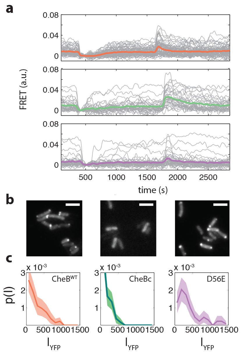
Example FRET time series and CheB localization.
(a) Example FRET time series for cells expressing CheB (top, pink), CheB (bottom,purple) , CheB (middle, green) in ΔCheB (VS124) background. (b) Localization of CheB in the cell probed by mVenus fusions to CheB. Clustering was quantified by the fraction of cells clearly showing one or more clusters in the cell. Shown are representative examples of CheB (left, 78% clustered), CheB (middle, 0%), CheB (right, 72% ). Scale bars 2 μm. (c) Histograms of fluorescence intensity for single cells in units of photons/pixel. Mean and standard deviation of these distributions for the strains is (from left to right) 272±237 (114 cells), 148±133 (150 cells) and 398±328 (106 cells). This corresponds to a CV of 0.87, 0.90, 0.82 for the three CheB genotypes, respectively. These cellular fluorescence intensities are corrected for inhomogeneous illumination as well as differences in cell area, and thus can be considered proportional to the cellular concentration of the respective cheB gene products.
Figure 3—figure supplement 2
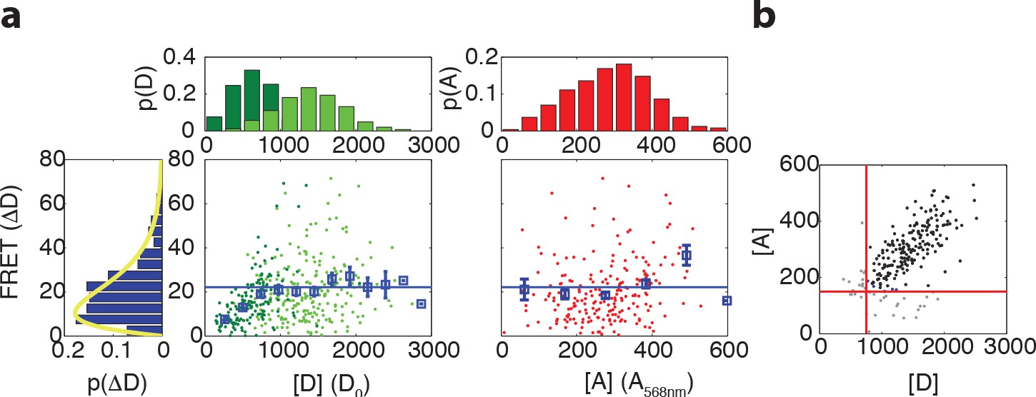
Relation between maximum FRET response and expression levels of donor and acceptor fluorophores.
(a) (Left) Scatter plot with donor intensity (D, green) versus FRET response to 500 μM MeAsp (ΔD) and (right) acceptor intensity (A, red, measured by direct excitation) with marginal distributions for A, D and ΔD in VS104/pSJAB12. For the donor intensity we measured at low induction (10 μM IPTG, dark green) and high induction (100 μM IPTG, light green). The acceptor intensities were only measured at high induction. In the scatter plots the mean FRET response is plotted with the error bars (blue), the horizontal line indicating the average for the binned data as described in panel (b). The yellow curve is a fit to a gamma distribution with corresponding values and 95% confidence intervals of and . All fluorescent intensities are measured in photons/pixel, are divided by cell size (area) and corrected for inhomogeneous illumination. All histograms are normalized to the number of cells. (b) Gating of the data. Scatter plot of donor intensity versus acceptor intensity. All data with fluorescent intensities (in photons/pixel) lower than D = 750 or A = 175 are excluded from the analysis since the FRET response depends on donor and acceptor intensity levels below these levels. The distribution of the FRET response (extreme left) is only for the gated data.
Figure 3—figure supplement 3
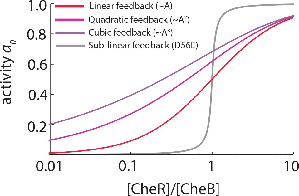
Linear and supralinear models of CheB feedback cannot explain bimodality in .
As explained in the main text, bimodality in the steady-state receptor-kinase activity could be explained by a steep transfer function mapping the expression-level ratio of adaptation enzymes to . Shown here are for models of the form , in which and represent the (de)methylation rates due to CheR and CheB, respectively, and the dependence of and on is (supra)linear (as discussed e.g. by [Clausznitzer et al., 2010]). The steady-state relation for each case is found by solving (see Materials and methods). In all three models the same CheR-dependent methylation is considered, and CheR and CheB are assumed to have the same catalytic rates . In the absence of phosphorylation, the CheB-dependent feedback depends linearly on the receptor-kinase activity (, red) while CheB phosphorylaton is modeled as quadratic (, light purple) or cubic (, purple) dependence. While phosphorylation feedback clearly decreases the slope of , the steepness of is greatly attenuated for these models with (supra)linear feedback, compared to the case with sublinear feedback (Equation 18, grey curve). To explain -bimodality with these shallow transfer functions of the (supra)linear models, one would need variability in the expression-level ratio [R]/[B] to span a range much greater than 102-fold, which is unlikely given the measured variability in expression level of chemotaxis genes (Kollmann et al., 2005; Yoney and Salman, 2015).
Figure 3—figure supplement 4
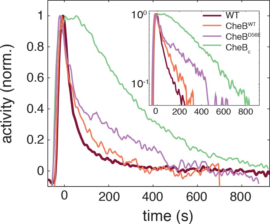
Phosphorylation feedback is not a necessary condition for fast removal adaptation dynamics.
Population FRET time series of cells expressing CheB-WT (orange), CheB-D56E (purple) , CheBc (green) in ΔCheB (VS124) background as well as WT (CheB from native chromosome position, VS104, brown) are shown after removal of 500 μM to which cells have adapted. The strain expressing CheB lacks phosphorylation feedback but has a fast removal response. The population FRET experiment is performed as described previously (Sourjik and Berg, 2002a). The strains and induction levels are the same as in the single-cell FRET experiments on the CheB mutants.
Figure 3—figure supplement 5

Phosphorylation defective mutants show impaired chemotaxis on soft agar.
Dark-field images after 14 hr of growth and motility on soft agar plates (0.26 % agar in TB with appropriate antibiotics, kept at 33.5 C). The different strains express either WT CheB, CheB-D56E and CheBc from an arabinose inducable pBAD plasmid in ΔCheB strain (UU2614). The arabinose concentration is varied from 0% to 0.001%
Figure 4 with 3 supplements
Temporal fluctuations in WT cells due to stochastic activity of adaptation enzymes CheR/CheB.
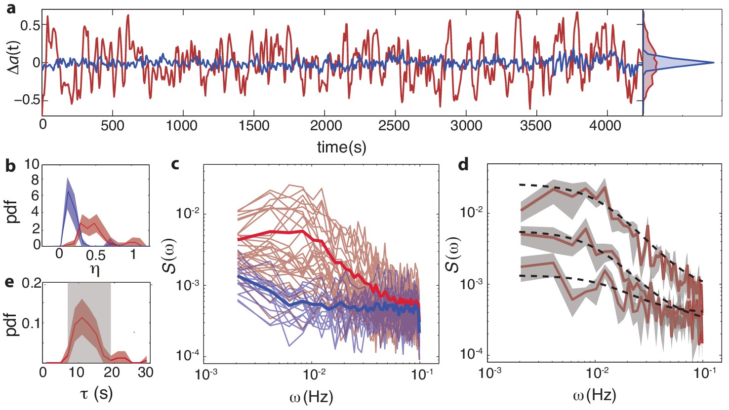
(a) Representative single-cell FRET time series of steady-state fluctuations Δa(t)=a(t)-a0 in WT cells (VS115, red), together with analogous data from CheRB- cells (TSS58,blue) for comparison (low-pass filtered with a 10 s moving average filter). (b) Histogram of fluctuation amplitude () for both WT (89 cells, red, from three independent experiments) and CheRB- (33 cells, blue, from two independent experiments), extracted from calculating the standard deviation of a low-pass filtered FRET time series over a 10 s window divided by the mean FRET level of a single cell. Shaded areas represent 95% confidence intervals obtained from bootstrap resampling. (c) Power spectral density (PSD) computed from single-cell FRET time series of 31 WT cells (red, from single experiment) and 17 CheRB- cells (blue, from single experiment), each from a single experiment. Thin curves in the lighter shade of each color represent single-cell spectra, and their ensemble average is shown as thick curves in a darker shade. The increased power at low-frequencies in WT cells was lost when PSD was computed after ensemble-averaging the time series Figure 4—figure supplement 1, indicating that these slow fluctuations are uncorrelated across cells. (d) Representative single-cell PSDs and fits by an Ornstein-Uhlenbeck (O–U) process. Shown are O-U fits (Lorentzian with constant noise floor; dashed curves) to three single-cell PSDs (solid curves). Shaded areas represent standard errors of the mean for PSDs computed from nine non-overlapping segments of each single-cell time series. Fits to all cells from the same experiment are shown in (Figure 4—figure supplement 2). Noise amplitudes computed from the O-U fit parameters (Figure 4—figure supplement 3) demonstrate excellent agreement with those computed directly from the time series (panel b). (e) Histogram of fluctuation timescales extracted from O-U fits to single-cell PSDs (red, 75 out of 89 cells). Cells without a clear noise plateau at low frequencies were excluded from the analysis (Figure 4—figure supplement 3). Red shaded region represents 95% confidence intervals obtained from bootstrap resampling. The gray shaded region indicates the variability (mean±std) that can be explained by experimental noise and a finite time window, obtained from simulated O-U time series (see Materials and methods).
-
Figure 4—source data 1
Source data (.mat) file containing FRET data and analysis.
- https://doi.org/10.7554/eLife.27455.024
Figure 4—figure supplement 1
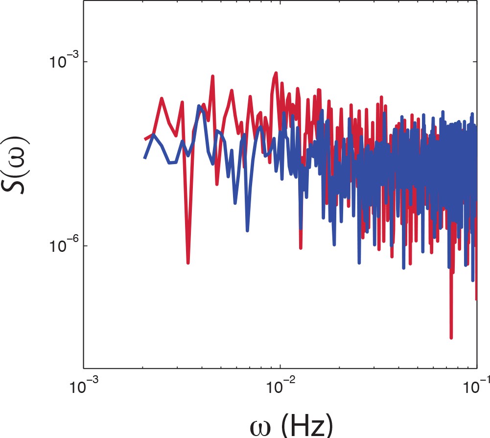
PSD estimates from population-averaged time series.
Power spectral density estimates from population averaged time series of CheRB+ (red) and CheRB- cells (blue). The time series are from the same experiment as shown in Figure 4c.
Figure 4—figure supplement 2
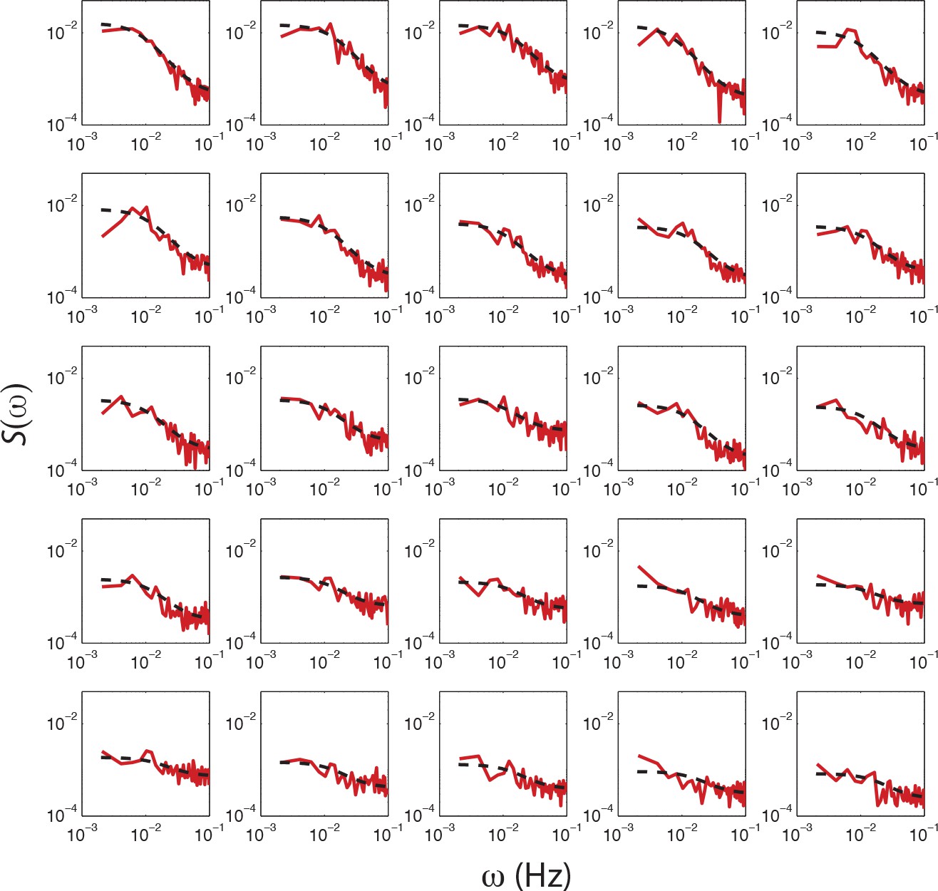
Fits of OU process to PSD estimates from single-cell FRET time series from a single experiment.
PSD estimates obtained from single-cell FRET time series (red dashed curve) with fits of O-U process to PSD estimates to 25 out of 31 cells (black dashed curve) from a single experiment shown in Figure 4c. The cells are sorted by variance calculated from the fit (cτ/2), with top-left having the highest. Cells without a clear low frequency plateau, higher than five times the standard deviation of the high frequency noise, were excluded from the analysis.
Figure 4—figure supplement 3
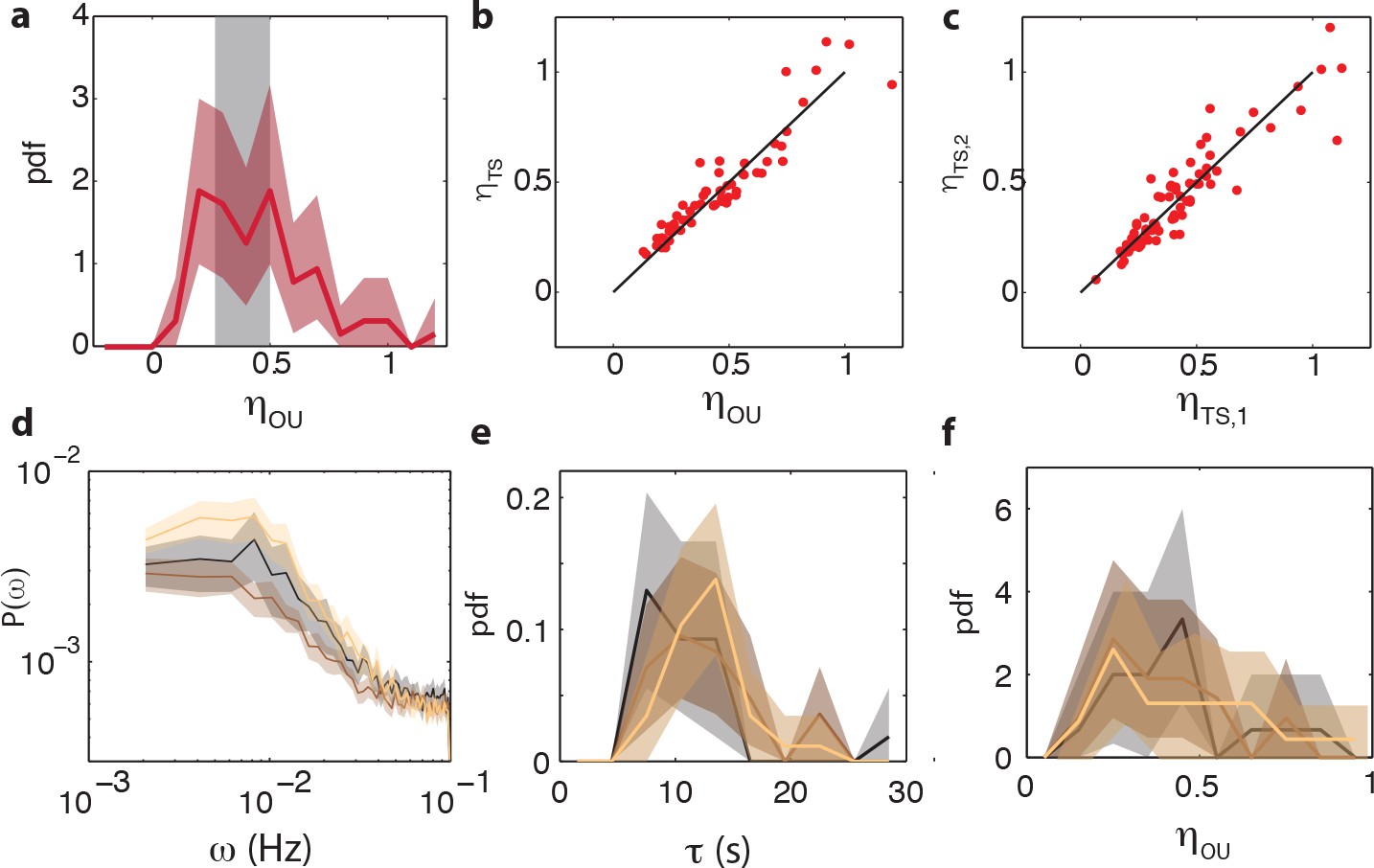
Comparison between noise amplitudes obtained from time series and power spectra and reproducibility of noise characteristics between different experiments.
(a) Noise amplitude for 75 CheRB+ cells time series (from three experiments) obtained with mean noise level of 0.42. 14 cells without a clear low frequency noise plateau, at least five times the standard deviation of the high frequency noise floor of the power spectrum, were excluded from the analysis because τ could not be constrained by the fit. The grey shaded area indicates the expected noise amplitude variability based on a finite time window and experimental noise in the experiment (see Materials and methods). The width is defined as the mean plus (minus) one standard deviation of the distribution of noise amplitudes obtained from simulated OU time series. (b) Noise amplitude obtained from fits of Ornstein-Uhlenbeck process to power spectra versus the noise amplitude obtained through calculating the standard deviation of the FRET time series after 10 s average filtering. Also shown is the diagonal . (c) The noise amplitude of the first () and second half () of the time series show high correlation, indicating that fluctuations are constant throughout the experiment. All noise amplitudes are defined as coefficient of variance. (d) Power spectrum density estimates for three independent experiments on CheRB+ cells (VS115), each based on 29 (gold), 28 (brown) and 18 cells (black). Shaded areas represent 95 % confidence intervals (2 s.e.). (e) Fluctuation timescale τ obtained from fits of Ornstein-Uhlenbeck process to single-cell power spectra. (f) Noise amplitude for the three different experiments.
Figure 5 with 3 supplements
Temporal fluctuations in adaptation-deficient cells depend strongly on activity and composition of chemoreceptor population.
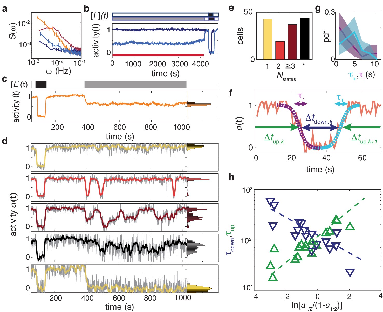
(a) Power spectral density (PSD) for temporal signal fluctuations during sub-saturating ligand stimulation of 18 cells with wild-type receptor complement (light blue, CheRB-, TSS58) and 58 cells expressing only chemoreceptor Tsr (orange, CheRB- Tsr+, TSS1964/pPA114). Also shown, for comparison, are PSDs from experiments without ligand stimulation for WT cells and CheRB- cells (red and dark blue, respectively; same data as in Figure 4). Error bars represent standard error of the mean. We note that the Tsr+ experiment had a larger FRET amplitude scaling factor (see Materials and methods) compared to the standard conditions under which the other strains were measured, and to account for this difference, the Tsr+ power spectrum has been scaled by a factor , where to account for this difference. (b) (Top) Stimulus protocol for modulation of the L-serine ligand concentration ([L](t)). Cells were incubated either in buffer ([L]=0, white) or a subsaturating stimulus ([L] = 50 μM, gray) for 1> hr. A saturating stimulus ([L] = 1 mM, black) is applied at the end of the experiment. (Bottom) Population- averaged time series for adaptation-deficient cells with wildtype receptor complement (CheRB-, TSS58) for experiments with (18 cells, light blue) and without (17 cells, dark blue) a sustained 50 μM L-serine stimulus during the time interval used to compute the PSDs in panel a (indicated by the red bar). (c) (Top) Stimulus protocol for L-serine concentration ([L](t)). At the start of the experiment, a saturating concentration ([L] = 1 mM, black) is applied for a short time. After flushing buffer ([L]=0, white), an intermediate concentration ([L] = 25 μM, gray) is sustained for 10 min. (Bottom) Population-averaged time series of 58 adaptation-deficient cells expressing Tsr as the sole chemoreceptor (RB-Tsr+; TSS1964/pPA114) under the stimulus protocol indicated above. (d) Selected single-cell time series of the population shown in panel (c), each normalized to its activity level before adding the first stimulus. To the unfiltered data (gray) a 7 s moving average filter is applied and superimposed (colored according to categories in panel (e)). All time series and corresponding activity histograms of the same experiment are shown in Figure 5 - Supplement 1 and 5. (e) Classification of RB-Tsr+ single cell fluctuation phenotypes by the number of stable activity levels observed during the sustained subsaturating stimulus. Many cells show only one stable activity level (yellow), corresponding to either full-amplitude response () or no response (). Some cells show two (red) or more (purple) apparently stable states. In other cells, fluctuations appeared chaotic with no discernibly stable state (black). (f) Definitions for analysis of two-state switching dynamics. The transition timescales and were determined by fits of a symmetric exponential function (see main text) to the upward (cyan) and downward (purple) switching transients, respectively. Residence times were defined as the interval between two successive transitions, at 50 activity. (g) Histogram of transition timescales, (4.2 ± 2.2 s, 26 events, cyan) and (3.5 ± 3.2, 29 events, purple) from 10 two-state switching cells of a single experiment with 1 Hz acquisition frequency. (h) Mean residence times and for two-state switching cells as a function of the average activity bias . The slopes are and , and the crossover point at s defines a characteristic switching timescale. Data of 17 cells from three independent experiments (one at 1 Hz acqusition, two at 0.2 Hz acquisition).
-
Figure 5—source data 1
Source data (.mat) file containing FRET data and analysis.
- https://doi.org/10.7554/eLife.27455.028
Figure 5—figure supplement 1
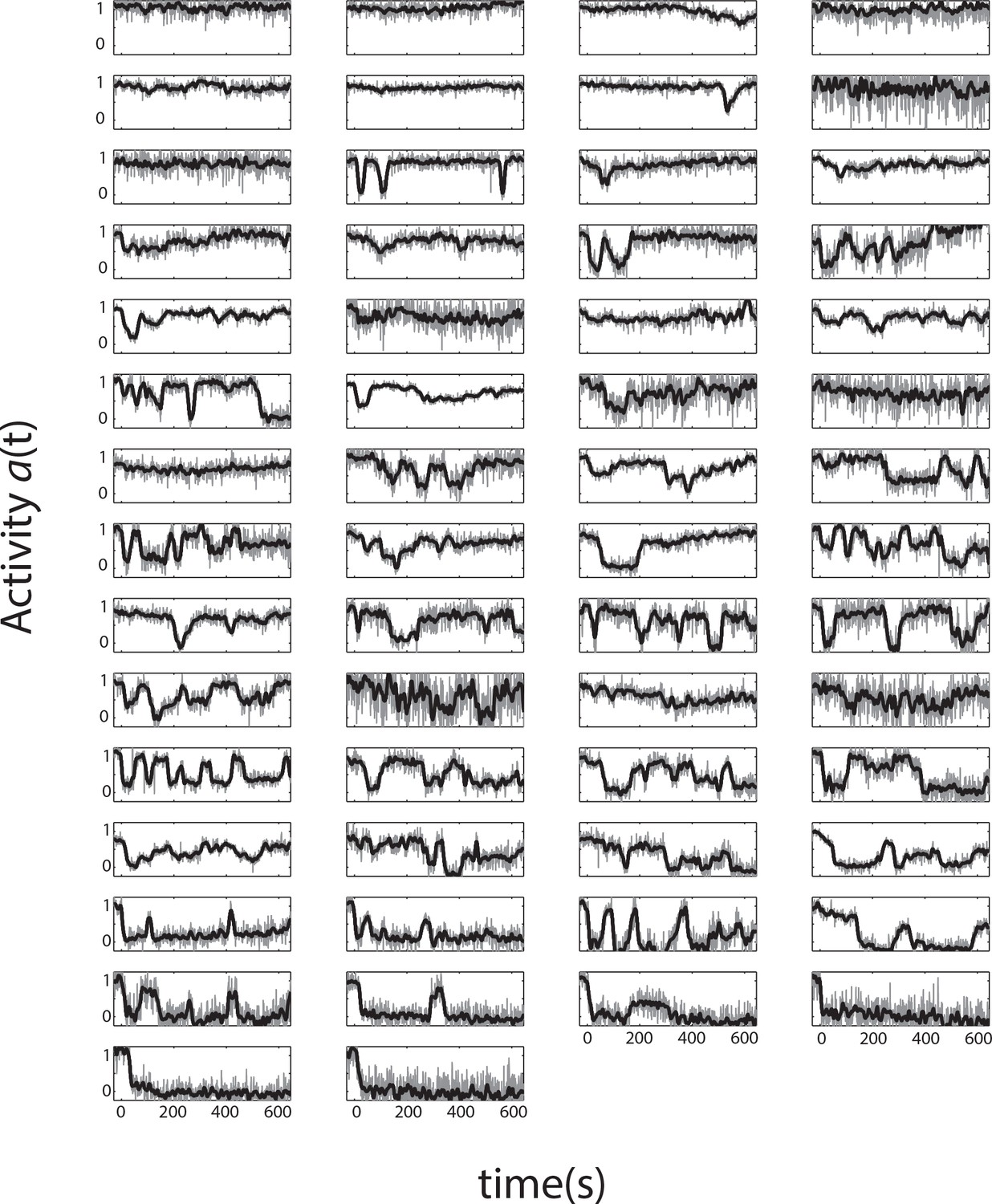
All single-cell time series from a single representative experiment.
Single-cell activity time series during a FRET experiment with a sustained ligand stimulus that elicits a population response of . Shown are 58 cells expressing Tsr as the sole chemoreceptor in CheRB- background (TSS1964) exposed to a step stimulus of 25 μM L-serine, each normalized to their own response amplitude. Time 0 is set to the time at which the population-averaged signal starts responding to a stimulus. The panels are ordered by the average activity level over the plot range.
Figure 5—figure supplement 2
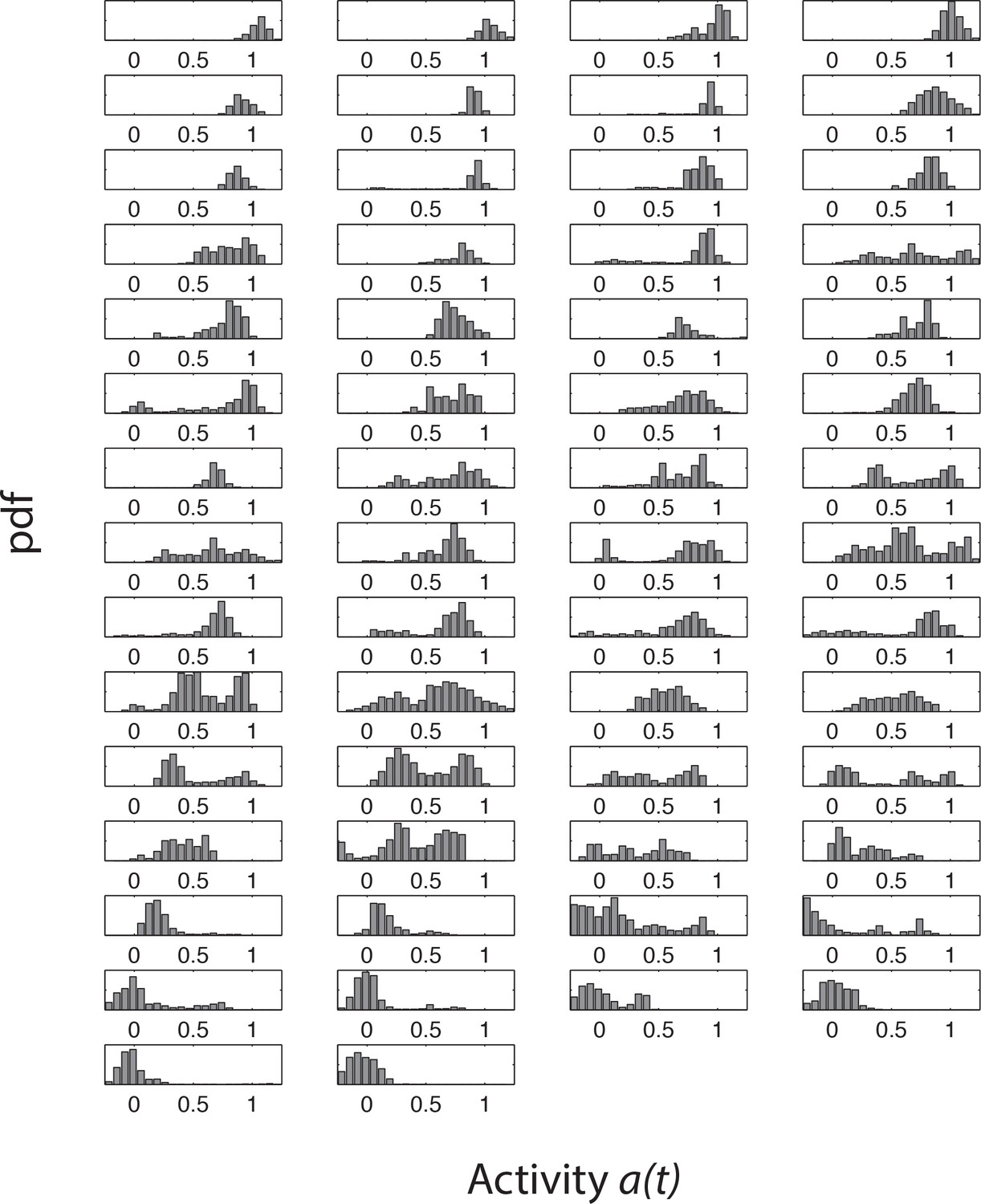
Histograms of activity during attractant stimulation for all cells from a single representative experiment.
Single-cell activity histograms from the same experiment as in Figure 5—figure supplement 1. The order of the panels, corresponding to individual cells, are the same as in Figure 5—figure supplement 1.
Figure 5—video 1
Segmentation video of three cells showing stochastic switching dynamics.
(Left panels) Bright-field image of cell obtained at the onset of the experiment. (Middle panels) YFP and mRFP segmented images, corrected for bleaching, in which the ROI of each cell is defined as a rectangle of 17 by 17 pixels. Due to small focus drift the cell shape shows some change over the course of the time series. (Right panels). Sum of fluorescent intensities of YFP (green) and mRFP (red) from each ROI low-pass filtered with 3 s moving average filter show clear anti-parallel responses, leading to changes in the ratio YFP/mRFP (blue), while the ratio barely changes during parallel changes due to another cell moving trough the ROI (t750 seconds, middle row). y-axis has arbitrary units. Acquisition rate is 1 Hz, every second image is shown.
Tables
Table 1
Variability in signaling parameters reported in this study with 95 CI obtained by bootstrap resampling.
N.D.: Not determined; N/A: Not applicable.
| Parameter | Genotype | Literature | ||
|---|---|---|---|---|
| CheR,CheB | CheRB+ | CheRB- | CheRB- | |
| Chemoreceptors | + (all) | + (all) | Tsr+ | |
| 0.23 0.06 | N/A | N/A | ||
| 0.20 0.06 | N/A | N/A | 0.18–0.5* | |
| 0.40 0.10 | N/A | N/A | ||
| N.D. | 0.49 0.09 | 0.16 0.07 | ||
| 0.44 0.12 | 0.09 0.04 | 0.49 0.09 | >0.2† | |
| 0.52 0.08 | 1.25 0.60 | 0.64 0.12 | ||
Table 2
Strains used in this study.
https://doi.org/10.7554/eLife.27455.031| Background | Plasmids | |||
|---|---|---|---|---|
| Strain | Source | Relevant genotype | Plasmid 1 | Plasmid 2 |
| VS115 | V. Sourjik | YZ FliC | pSJAB106 | pZR1 |
| VS104 | Sourjik and Berg, 2002a | CheYZ | pSJAB12 | pBAD33 |
| TSS58 | this work | RBYZ FliC | pSJAB106 | pZR1 |
| VS149 | Sourjik and Berg, 2004 | RBYZ | pVS12 | pVS33 |
| VS124 | Clausznitzer et al., 2010 | CheBYZ | pSJAB12 | pVS112 |
| VS124 | CheBYZ | pSJAB12 | pVS97 | |
| VS124 | CheBYZ | pSJAB12 | pVS91 | |
| UU2567 | Kitanovic et al., 2015 | CheRBYZ,MCP† | pSJAB106 | pPA114 Tsr |
| TSS1964 | this work | CheRBYZ,MCP FliC* | pSJAB106 | pPA114 Tsr |
| UU2614 | J.S. Parkinson | CheB (4-345) | pTrc99a | pVS91,97,112 |
-
All strains are descendants of E. coli K-12 HCB33 (RP437). In all FRET experiments, strains carry two plasmids and therefore confer resistance to chloramphenicol and ampicillin.
†all five chemoreceptor genes tar tsr tap trg aer deleted.
-
*expresses sticky FliC filament (Scharf et al., 1998)
Table 3
Plasmids used in this study.
https://doi.org/10.7554/eLife.27455.032| Plasmid | Product | System | Ind | Res | Source |
|---|---|---|---|---|---|
| pVS52 | CheZ-5G-YFP | pBAD33 | ara | cam | Sourjik and Berg, 2002a |
| pVS149 | CheY-5G-mRFP1 | pTrc99a | IPTG | amp | Sourjik and Berg, 2002a |
| pSJAB12 | CheZ-5G-YFP/CheY-5G-mRFP1 | PTrc99a | IPTG | amp | This work |
| pSJAB106 | CheZ-5G-YFP/CheY-5G-mRFP1¶ | PTrc99a | IPTG | amp | This work |
| pVS91 | CheB† | pTrc99a | ara | cam | Liberman et al., 2004 |
| pVS97 | CheB-D56E‡ | pBAD33 | ara | cam | Clausznitzer et al., 2010 |
| pVS112 | CheBc§ | pBAD33 | ara | cam | V. Sourjik |
| pSJAB 122 | CheBc-GS4G-mVenus | pBAD33 | ara | cam | This work |
| pSJAB 123 | CheB(D56E)-GS4G-mVenus | pBAD33 | ara | cam | This work |
| pSJAB 124 | CheB-GS4G-mVenus | pBAD33 | ara | cam | This work |
| pZR 1 | FliC* | pKG116 | NaSal | cam | This work |
| pPA114 Tsr | Tsr | pPA114 | NaSal | cam | Ames et al., 2002 |
-
¶Contains a A206K mutation to enforce monomerity..
†expresses WT CheB.
-
‡carries a point mutation D56E in CheB.
§expresses only residues 147–349 of CheB, preceded by a start codon (Met).
-
*expresses sticky FliC filament (Scharf et al., 1998)
Table 4
List of global parameters used for model of Mello and Tu.
In these fits, is a free parameter while others are constrained ±5% by published values.
| Parameter | Start value (Mello and Tu, 2007) | Final value |
|---|---|---|
| 0.314 | 0.29 | |
| 0.80 | 0.84 | |
| 1.23 | 1.29 | |
| 1.54 | 1.61 | |
| – | 21.2 μM |
Table 5
List of parameters used for Goldbeter-Koshland description of CheB phosphorylation feedback.
https://doi.org/10.7554/eLife.27455.034| Parameter | Value | Literature | Source |
|---|---|---|---|
| 1 | 0.75 | Shimizu et al., 2010 | |
| 2 | Kentner and Sourjik, 2009 | ||
| 0.03 | <<1 | Emonet and Cluzel, 2008 | |
| 0.03 | <<1 | Emonet and Cluzel, 2008 | |
| 0.2 | <<1 | ||
| M (WT) | 15 | 100 | Anand and Stock, 2002 |
| M (CheBc) | 7 | 15 | Simms et al., 1985 |
Additional files
-
Transparent reporting form
- https://doi.org/10.7554/eLife.27455.035
Download links
A two-part list of links to download the article, or parts of the article, in various formats.
Downloads (link to download the article as PDF)
Open citations (links to open the citations from this article in various online reference manager services)
Cite this article (links to download the citations from this article in formats compatible with various reference manager tools)
Phenotypic diversity and temporal variability in a bacterial signaling network revealed by single-cell FRET
eLife 6:e27455.
https://doi.org/10.7554/eLife.27455


