Monitoring ATP dynamics in electrically active white matter tracts
- Max-Planck-Institute for Experimental Medicine, Germany
- University of Zurich, Switzerland
- University of Leipzig, Germany
- Kyoto University, Japan
- Center Nanoscale Microscopy and Molecular Physiology of the Brain, Germany
Figures
Figure 1
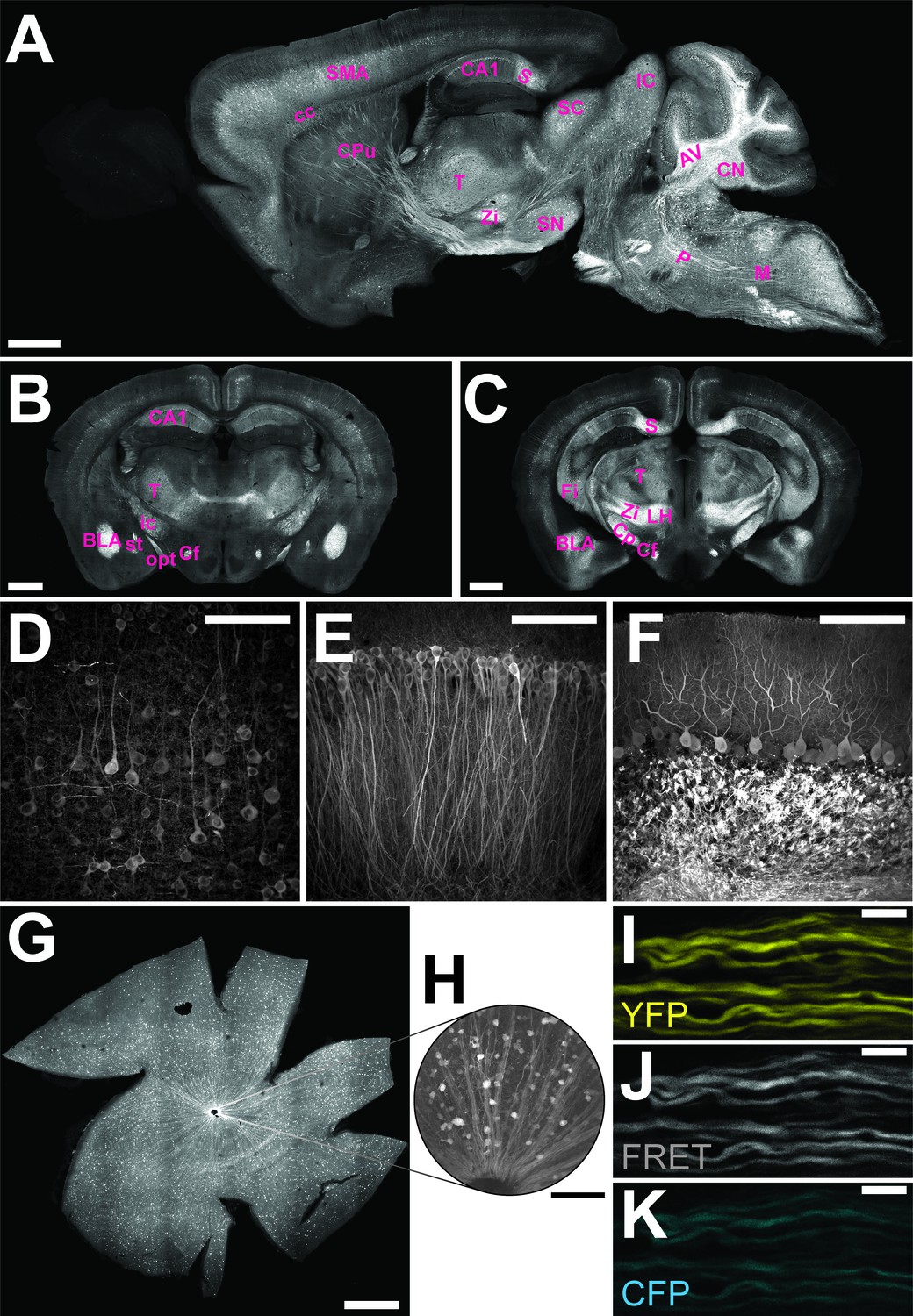
Characterization of the expression pattern of the newly generated B6-Tg(Thy1.2-ATeam1.03YEMK)AJhi (ThyAT)-mouse line.
(A) Sagittal section of the brain highlights broad ATeam1.03YEMK expression in neurons in almost all brain regions with the exception of the olfactory bulb. Scale bar: 1 mm. (B,C) ThyAT expression pattern in coronal brain sections revealing sensor expression e.g. in thalamus, hypothalamus, amygdala, cortex and hippocampus. Scale bar: 1 mm. Abbreviations used in panels A–C are: AV: arbor vitae; BLA: basolateral amygdalar nucleus, anterior; CA1: CA1 region of the hippocampus; cc: corpus callosum; Cf: columns of the fornix; CN: cerebellar nuclei; Cp: cerebral peduncle; CPu: caudate putamen; Fi: fimbria; IC: inferior colliculus; ic: internal capsule; LH: lateral area of the hypothalamus; M: medulla; opt: optic tract; P: pons; S: subiculum; SC: superior colliculus; SMA: somato-motor area (cortex); SN: substantia nigra; st: stria terminalis; T: thalamus; Zi: zona incerta (thalamus). (D) Within the cortex, neurons expressing ATeam1.03YEMK are clearly visible including their processes. Note the lack of ATP-sensor localization to the nucleus. Scale bar: 100 μm. (E) Also in the hippocampus neurons strongly express ATeam1.03YEMK. Scale bar: 100 μm. (F) In the cerebellum, Purkinje cells express the ATP-sensor. In addition, incoming mossy fibers strongly express ATeam1.03YEMK. Scale bar: 100 μm. Images in panels A, D–F are obtained on brain slices from a four month old animal, images in panels B and C are from mice at the age of two month. (G) Expression pattern of the ATP-sensor in the retina. Thy1.2 promoter drives the expression of ATeam1.03YEMK in ganglion cells. Scale bar: 1 mm. (H) Magnified view of neurons and axons in the retina expressing ATeam1.03YEMK. Scale bar: 100 μm. (I–K) Representative images of optic nerve axons showing the YFP channel (I), FRET channel (J) and CFP channel (K). The ATeam1.03YEMK expression is present in different axons independent of their diameter. Scale bar: 10 μm.
Figure 2
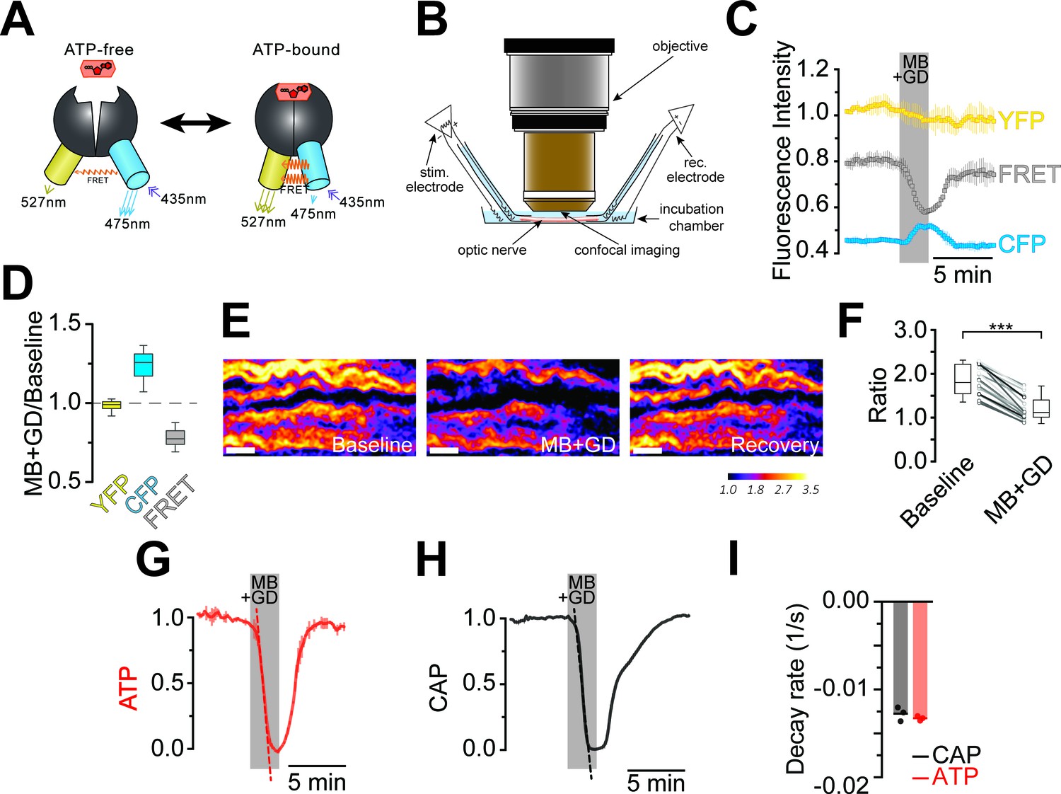
Imaging of ATP combined with electrophysiology in acutely isolated optic nerves of ThyAT-mice.
(A) Binding of ATP induces a conformational change in the genetically encoded ATP-sensor ATeam1.03YEMK thus increasing the FRET effect (YFP emission upon CFP excitation) and simultaneous decreased emission of CFP (upon CFP excitation). The ratio between FRET and CFP can thus be correlated with the concentration of ATP present in the cell. (B) Schematic representation of the set-up to acquire evoked CAPs in the optic nerve and to simultaneously investigate relative ATP levels by electrophysiology and confocal imaging, respectively. (C) Time course of fluorescence intensity recorded in the YFP, FRET and CFP- channels during application of mitochondrial blockage (MB) and glucose deprivation (GD) for 2.5 min. Values are normalized to YFP intensity prior to application of MB+GD (n = 3 nerves). Time resolution: 10.4 s. (D) The combination of MB and GD is a fast and reliable way to deplete ATP in axons of the optic nerve. ATP depletion is measured as a decrease in FRET and increase in CFP, calculated as ratio between fluorophore intensity during MB+GD, over fluorophore intensity at baseline condition (MB+GD/Baseline). Notably, YFP emission upon YFP excitation remains unchanged (n = 5 nerves). (E) Ratiometric images displaying the FRET/CFP ratio of the ATeam1.03YEMK–sensor in the axons of the optic nerve during ATP depletion following MB+GD. The phases before (Baseline) and after (Recovery) are also shown. Scale bar: 10 μm. (F) FRET/CFP ratio values (not normalized) during baseline and MB+GD. The boxplots show summarized data of n = 19 nerves, lines in between boxplots show changes in the FRET/CFP ratio of all 19 individual nerves (***p<0.001). (G) To assess ATP variations, the ratio of the fluorescence intensities of the FRET and CFP-channel was calculated (FRET/CFP ratio) and normalized to baseline (set as 1) and MB+GD (set as 0). The red dashed line visualizes the slope of ATP drop at the point of maximal velocity of ATP decay during mitochondrial blockage (MB+GD, n = 3). (H) Recording of the evoked compound action potential (CAP), given as the normalized curve integral during mitochondrial blockage and glucose deprivation (MB+GD). The black dashed line represents the slope at the point of maximal velocity of CAP changes during MB+GD treatment (n = 3). Individual CAP traces are shown in Figure 3—figure supplement 1. (I) Stripe plot describing CAP (black) and ATP (red) kinetics, expressed as maximal variation per s, during MB+GD (p=0.39, n = 3, Welch’s t-test). Dots show individual data points, bars and lines represent the mean of all data.
-
Figure 2—source data 1
Table containing data for Figure 2.
This xlsx-data file contains the data shown in Figure 2D,F and I.
- https://doi.org/10.7554/eLife.24241.005
Figure 3 with 2 supplements
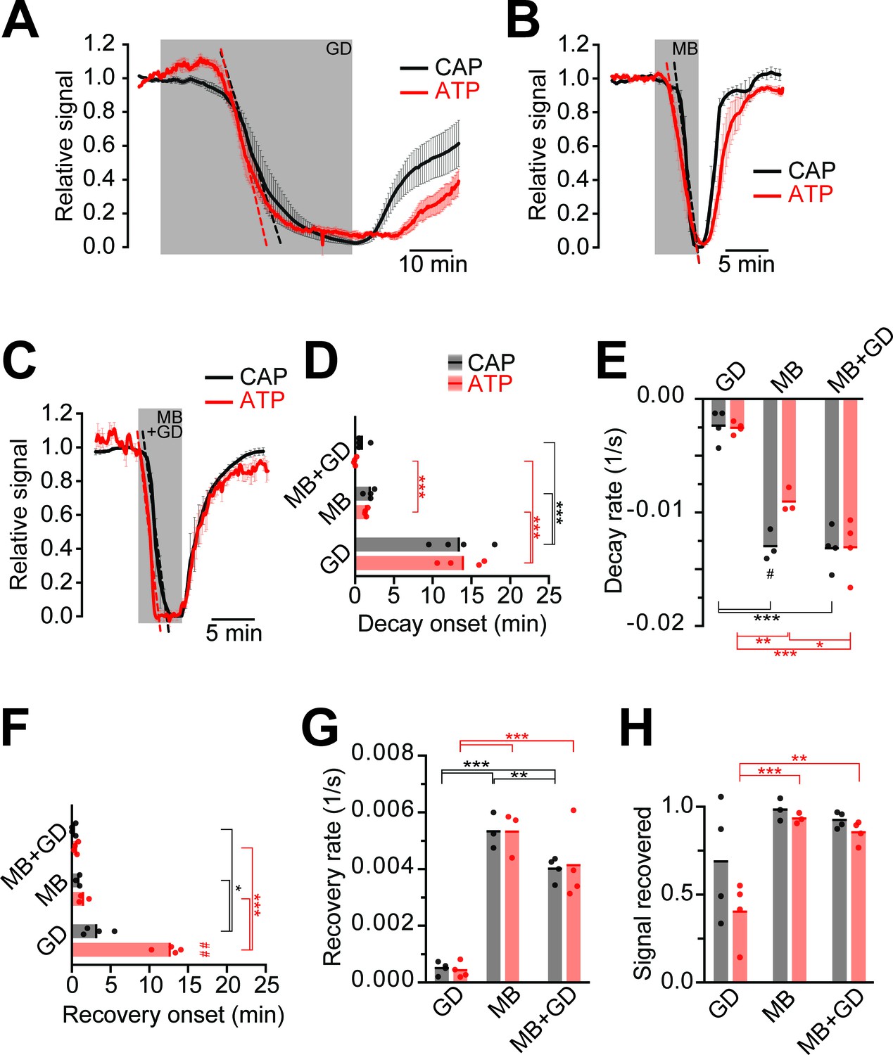
Impairment of axonal ATP and CAP by glucose deprivation and/or inhibition of mitochondrial respiration.
(A) Removal of glucose from the aCSF (glucose deprivation, GD, 45 min) induces similar ATP (red) and CAP (black) decays starting at around 13 min after onset of the treatment. Red and black dashed, straight lines represent the maximum velocity of ATP and CAP decay (also applies to panels B and C). When 10 mM glucose is restored, CAP recovery precedes ATP restoration (n = 4 nerves). (B) Blockade of mitochondrial respiration by azide (MB, 5 min) produces a fast decay in ATP (red) and CAP (black) starting at 1.8 min after beginning of treatment. When azide is removed, CAP and ATP are promptly restored, with CAP recovery preceding the ATP increase (n = 4 nerves). (C) Simultaneous removal of glucose and blockade of mitochondrial respiration with azide (MB+GD, 5 min) produces a fast decay in ATP (red) preceding CAP decay (black), starting already 0.5 min after onset of treatment. Following azide removal and replenishment of glucose, CAP and ATP are restored (n = 4 nerves). (D) Time of onset of the ATP or CAP decay. The slowest decay induction was observed during glucose deprivation. (E) Velocity of signal decay for ATP and CAP during each of the three treatments: glucose deprivation (GD), mitochondrial blockage (MB) and the combination of both (MB+GD). (F) Time of onset of ATP or CAP recovery after reperfusion with control aCSF containing 10 mM glucose. (G) Rate of recovery of both ATP and CAP during reperfusion of the nerves with aCSF containing 10 mM glucose after the treatments indicated. (H) Comparison of ATP and CAP area overall recovery after individual treatments. Data in D–H is presented as stripe plots, with dots representing individual data points, bars and lines showing the mean. Hash signs indicate statistically significant differences between ATP and CAP under the same condition (#p<0.05, ##p<0.01, paired t-test); asterisks on red (ATP) and black (CAP) lines indicate statistically significant differences between different conditions (*p<0.05, **p<0.01, ***p<0.001; one-way ANOVA with Newman-Keuls post-hoc test).
-
Figure 3—source data 1
Table containing data for Figure 3.
This xlsx-data file contains the data shown in Figure 3D–H and Figure 3—Figure supplement 2.
- https://doi.org/10.7554/eLife.24241.007
Figure 3—figure supplement 1
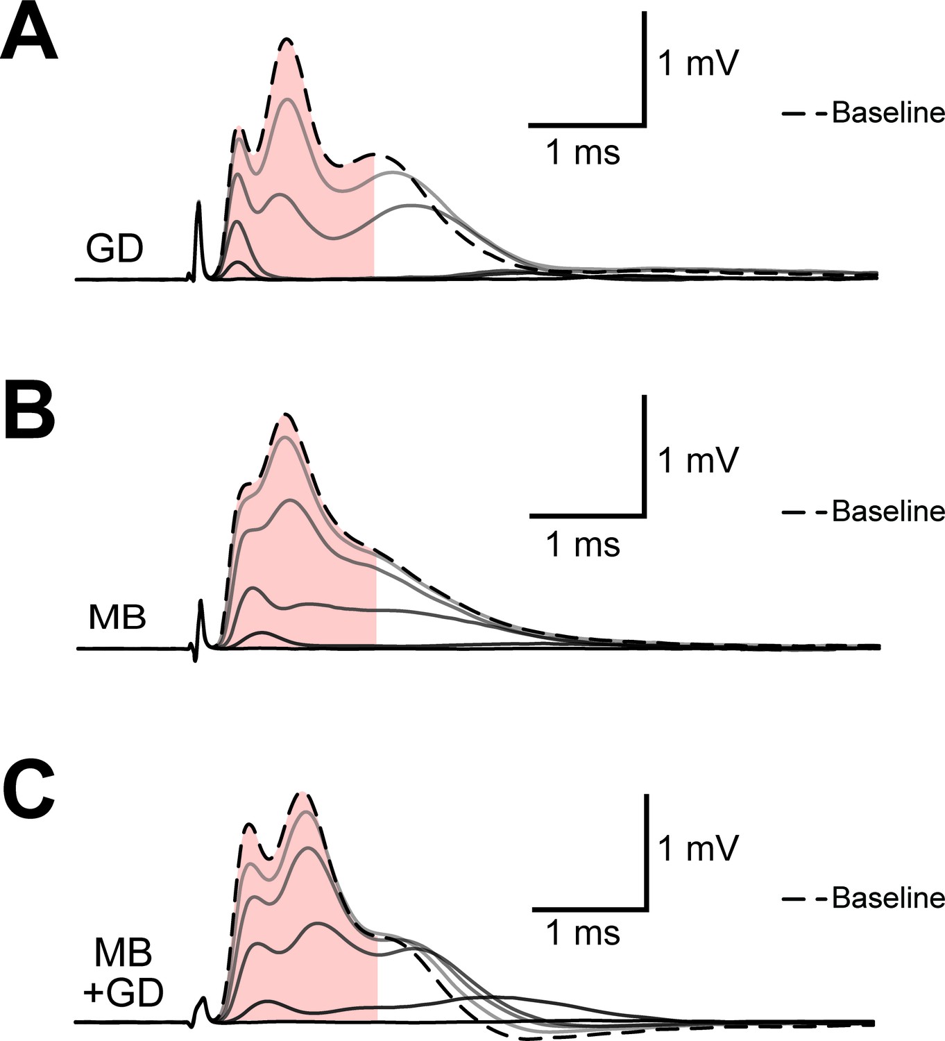
Example of progression of CAP traces’ decay during energy deprivation.
Shown are single traces obtained under control conditions (baseline, dashed line) as well as during application of GD (A, total 45 min), MB (B, total 5 min) or MB+GD (C, total 5 min). Single traces are separated by 330 s (A) or 30 s (B,C). The shaded area indicates the area under the CAP wave form used for CAP quantification for the baseline condition, the same time window was used for analysis of CAPs at later time points. Under all conditions, no CAP is elicited by electrical stimulation anymore at the end of the treatment.
Figure 3—figure supplement 2
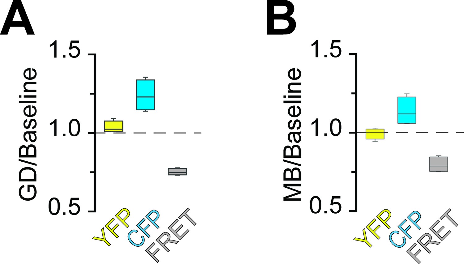
Analysis of fluorescence changes of the ATP sensor during application of different models of energy deprivation to optic nerves.
Changes of the fluorescence signal relative to the baseline signal during glucose deprivation (A; GD) or mitochondrial blockage (B; MB). Fluorescence intensities of the three recorded channels between 44.75 min and 45 min or 4.75 min and 5 min of incubation with GD and MB, respectively, were averaged (GD: n = 4 nerves; MB: n = 4 nerves). Compare Figure 2C,D for data on GD+MB. In all cases, fluorescence in the CFP channel increased, while fluorescence in the FRET channel decreased. Of note, YFP emission upon direct YFP excitation remains stable.
Figure 4 with 5 supplements
Comparison of ATP and CAP dynamics during high frequency stimulation.
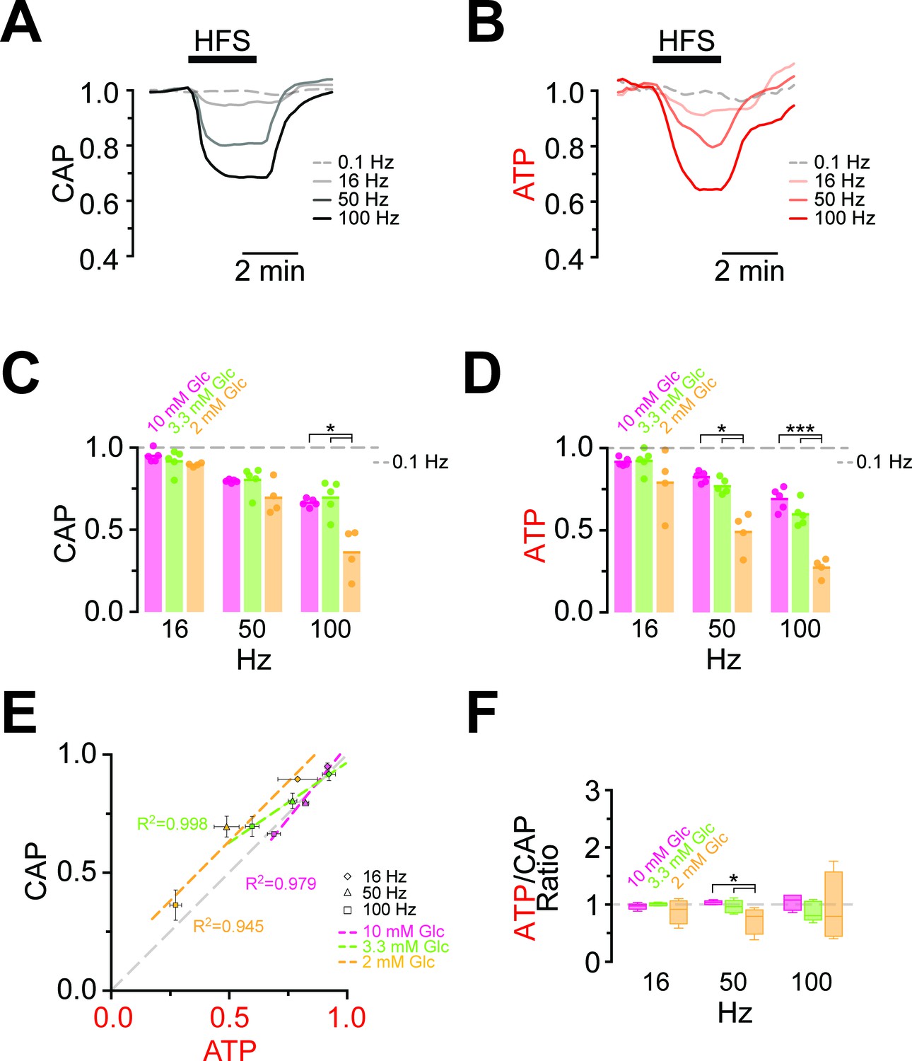
(A) The CAP area decreases over time during high-frequency stimulation (HFS). The decay amplitude deviates from the absence of HFS, indicated by the dashed line (0.1 Hz, used for normalization to 1.0), and increases progressively with the increase in stimulation frequency (16 Hz, 50 Hz, 100 Hz). Traces from one representative nerve incubated in aCSF containing 10 mM glucose are shown. (B) Axonal ATP levels also decrease with increasing stimulation frequency, reaching a new steady state level which depends on the stimulation frequency. Same experiment as in panel A. (C) Remaining CAP area at the end of the HFS (overall decay amplitude) during incubation of nerves in different glucose concentrations quantified during the last 30 s of HFS. The stripe plot shows summarized data from n = 5, 5, or 4 nerves for 10 mM, 3.3 mM and 2 mM glucose, respectively. The dashed line at 1 shows CAP size at 0.1 Hz stimulation frequency, which was used for normalization. (D) Quantification of ATP decay amplitude during incubation of the same nerves as in (C) in different glucose concentrations. The dashed line at 1 shows ATP levels at 0.1 Hz stimulation frequency. (E) Correlation of the amplitude of ATP and CAP decay during HFS of nerves bathed in aCSF containing the glucose concentrations indicated. Data points are very close to the diagonal of the graph indicating that ATP and CAP change by similar factors. (F) Ratio of ATP and CAP drop during HFS in the presence of glucose in the concentrations indicated. If both parameters change by the same factor, this ratio remains equal to one. Data in (C–D) is presented as stripe plots, with dots representing individual data points and bars and lines showing the mean. Asterisks indicate statistically significant differences between glucose concentrations (*p<0.05, ***p<0.001; Welch’s t-test).
-
Figure 4—source data 1
Table containing data for Figure 4.
This xlsx-data file contains the data shown in Figure 4C,D,F and Figure 4—Figure supplement 5.
- https://doi.org/10.7554/eLife.24241.011
Figure 4—figure supplement 1
Example of progression of CAP traces’ decay during high frequency stimulation (HFS).
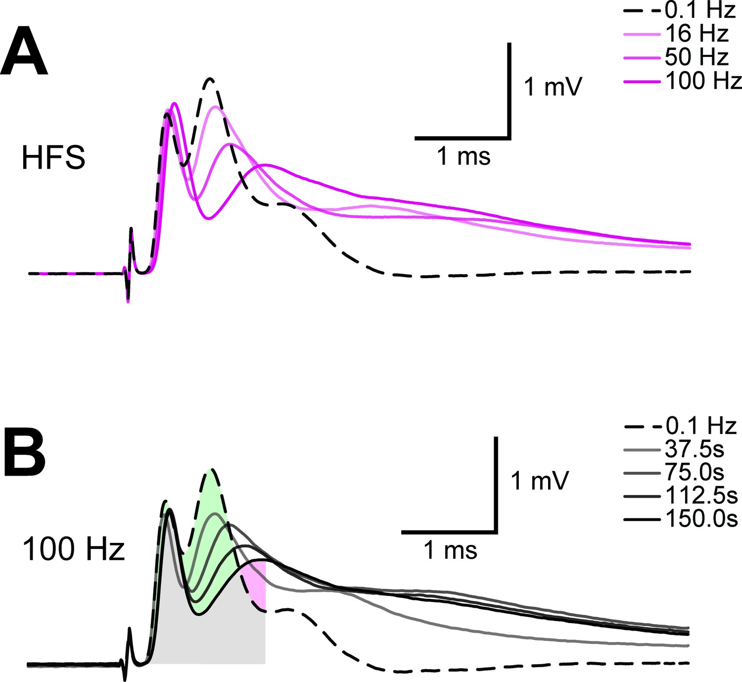
(A) The three peaks recognizable in the baseline trace (dashed line) are differently affected by increasing stimulation frequency and for CAP analysis only the first two are considered. Shown are single traces obtained prior to stimulation (baseline) as well as at the end of a 2.5 min stimulation period at different stimulation frequencies (16 Hz, 50 Hz, 100 Hz) of a nerve incubated in aCSF containing 10 mM glucose. (B) Example of progression of CAP from baseline (dashed line) during stimulation of an optic nerve at 100 Hz incubated in aCSF containing 10 mM glucose for a total stimulation time of 2.5 min. Single traces are separated by 37.5 s. The shaded area indicates the area under the CAP wave form used for CAP quantification for the baseline condition (green) and after 150 s of HFS (red). Grey shading results from the overlay of green and red shading.
Figure 4—figure supplement 2

Stimulation of optic nerves with progressively increasing frequencies.
Frequency-dependent changes in relative signal amplitude of ATP and CAP, during progressively increasing stimulation frequencies (1 Hz to 100 Hz) and following recovery. Nerves incubated in aCSF containing 10 mM glucose were stimulated for 45 s each with the indicated frequencies, directly followed by stimulation with the next higher frequency. The dashed line at 1.0 shows ATP and CAP values at 0.1 Hz stimulation frequency, which are used for respective normalization (n = 4 nerves).
Figure 4—figure supplement 3

Correlation of the rates and amplitudes of CAP and ATP changes during HFS in different glucose concentrations.
(A) Correlation of the velocity of the initial decay of CAP at the beginning of HFS and the amplitude of CAP decay at the end of HFS. The faster the CAP drops, the larger the CAP amplitude is. (B) Same analysis for ATP as for CAP area in panel A. Also a faster ATP consumption at the beginning of HFS coincides with a larger decrease in ATP signal amplitude. (C) Correlation of the rates of CAP area recovery after the cessation of stimulation and the amplitudes of CAP changes at the end of the stimulation at different glucose concentrations. The velocity of CAP recovery increases with larger amplitude of CAP decay during stimulation. (D) Same analysis as in C for ATP. ATP recovery rates are strongly depending on the amplitude of ATP decrease during HFS at 10 mM and 3.3 mM glucose, but much less in the presence of 2 mM glucose. The graphs summarize data from n = 5, 5, or 4 nerves for 10 mM, 3.3 mM and 2 mM glucose, respectively.
Figure 4—figure supplement 4
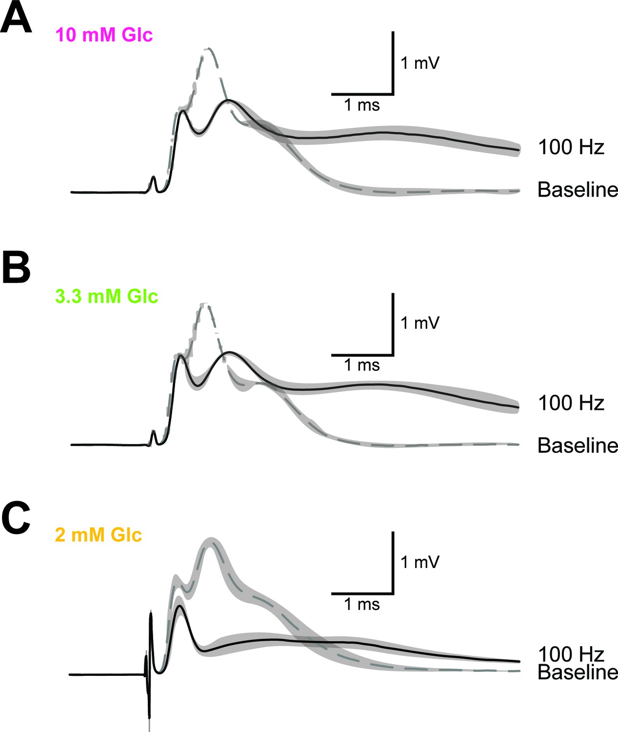
Example of CAP traces before and after high-frequency stimulation (HFS) of optic nerves incubated in aCSF with different concentrations of glucose.
Shown are mean CAP wave forms (n = 3 nerves for each condition) incubated in aCSF containing 10 mM glucose (A), 3.3 mM glucose (B) and 2 mM glucose (C) prior to high- frequency stimulation (‘baseline’; dashed lines) or at the end of the 2.5 min HFS (100 Hz) period (solid lines). Grey areas indicate SEM.
Figure 4—figure supplement 5
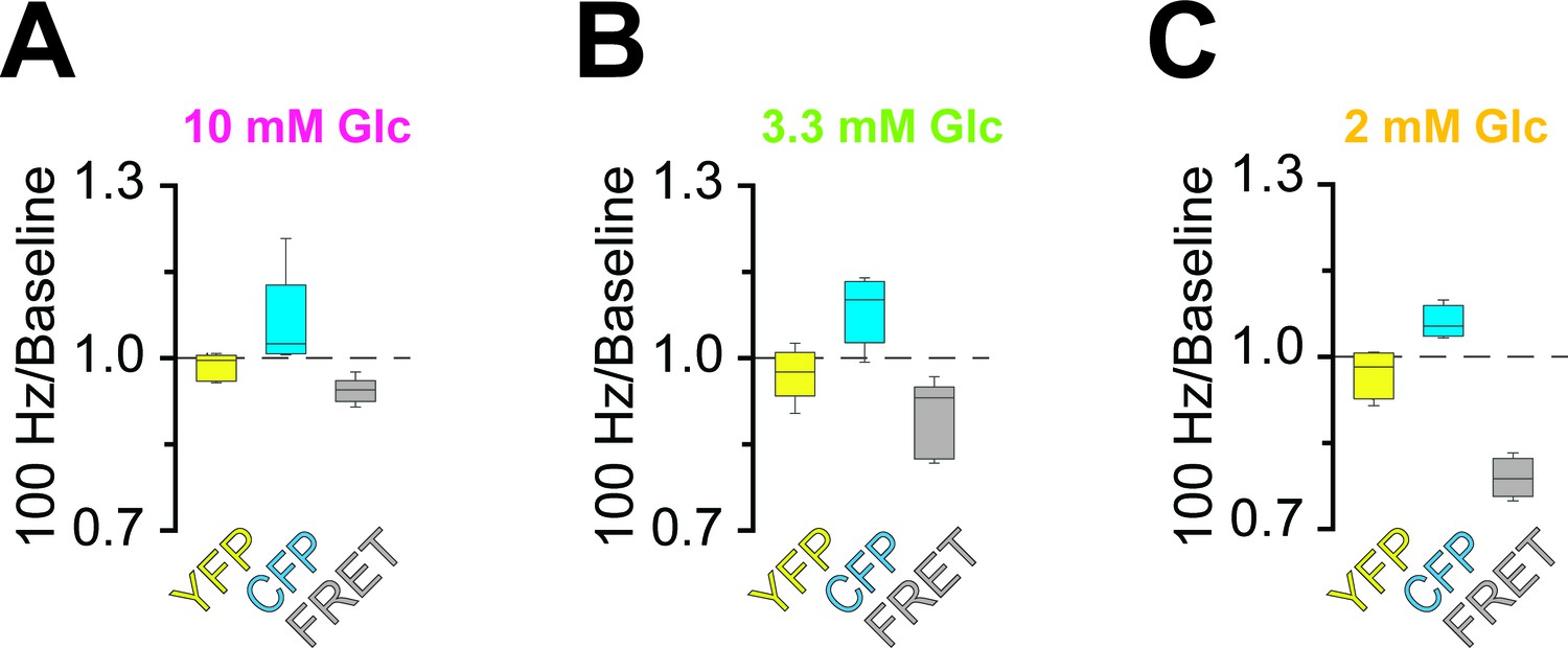
Analysis of fluorescence changes of the ATP sensor during high-frequency stimulation (HFS) of optic nerves incubated in aCSF with different concentrations of glucose.
Changes of the fluorescence signal at the end of the 2.5 min HFS (100 Hz) period relative to the baseline signal prior to stimulation of optic nerves incubated in aCSF containing 10 mM glucose (A), 3.3 mM glucose (B) and 2 mM glucose (C). During HFS, fluorescence in the CFP channel increased, while fluorescence in the FRET channel decreased. Of note, YFP emission upon direct YFP excitation remains stable. n = 5, 5, 4 nerves for 10 mM, 3.3 mM and 2 mM glucose, respectively.
Figure 5 with 2 supplements
Energy metabolism of optic nerves depends on the type and concentration of substrates and involves lactate metabolism.
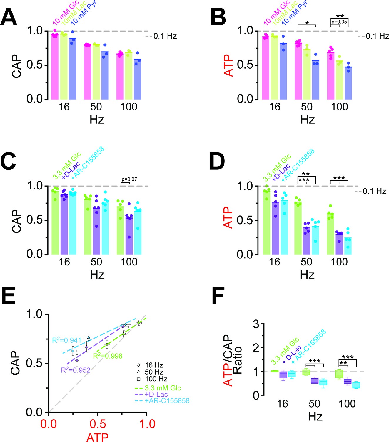
(A) The comparison between CAP area decay of optic nerves incubated in 10 mM glucose aCSF (n = 5 nerves) versus optic nerves incubated either in 10 mM lactate or 10 mM pyruvate (n = 3 nerves) during HFS, shows no significant differences among the three substrates (p>0.05, Welch’s t test). (B) In contrast, analysis of axonal ATP levels shows that at higher frequencies glucose is a better substrate to maintain axonal ATP levels. Same experiments as in panel A. (C) In the presence of glucose (3.3 mM; n = 5 nerves) as exogenous energy substrate, inhibition of lactate metabolism by D-lactate (20 mM; competitive inhibitor of endogenous L-lactate metabolism at MCTs and LDH, n = 6) or AR-C155858 (10 µM; MCT1 and MCT2 selective inhibitor, n = 6) does not significantly affect CAPs. (D) Analysis of ATP under the same conditions as in (C): ATP levels undergo a strong decrease at higher frequencies in the presence of D-lactate or AR-C155858. (n = 5 nerves for all conditions). The dashed lines in panels A–D at 1 show CAP size or ATP levels at 0.1 Hz stimulation frequency used for normalization. (E) Inhibition of metabolism of endogenously produced L-lactate in the presence of glucose as the sole exogenous energy substrate shifts the correlation of ATP and CAP to the upper left showing that ATP changes more strongly than CAP. (F) The ratio of ATP and CAP drop decreases significantly in the presence of inhibitors of lactate metabolism, confirming that ATP changes more strongly than CAP. Asterisks in (A–D and F) indicate significant differences among conditions: *p<0.05, **p<0.01, ***p<0.001; Welch’s t test.
-
Figure 5—source data 1
Table containing data for Figure 5.
This xlsx-data file contains the data shown in Figure 5A–D,F and Figure 5—Figure supplement 1B.
- https://doi.org/10.7554/eLife.24241.018
Figure 5—figure supplement 1
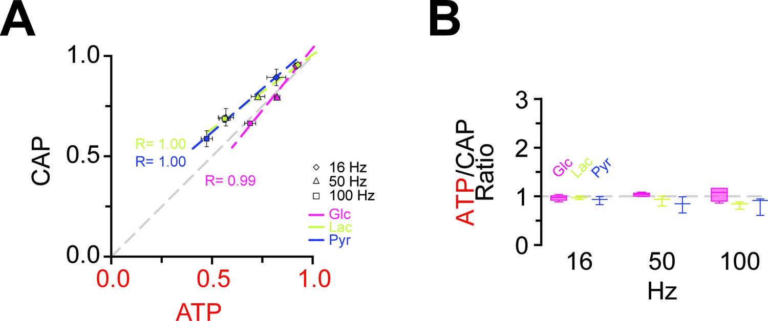
Correlation of the amplitudes of CAP and ATP changes in the presence of lactate and pyruvate as exogenous energy substrates.
(A) Correlation of ATP and CAP decay amplitude during HFS of nerves bathed in aCSF containing glucose, lactate or pyruvate (each 10 mM) as energy substrates. n = 5, 3, 3 nerves for glucose, lactate and pyruvate, respectively. (B) ATP to CAP amplitude ratio, calculated for nerves bathed in aCSF containing lactate (10 mM) or pyruvate (10 mM) as energy substrates during HFS. The ratio remains almost equal to one for all conditions supporting the notions that both ATP and CAP change by a similar factor. n = 5, 3, 3 for glucose, lactate and pyruvate, respectively.
Figure 5—figure supplement 2
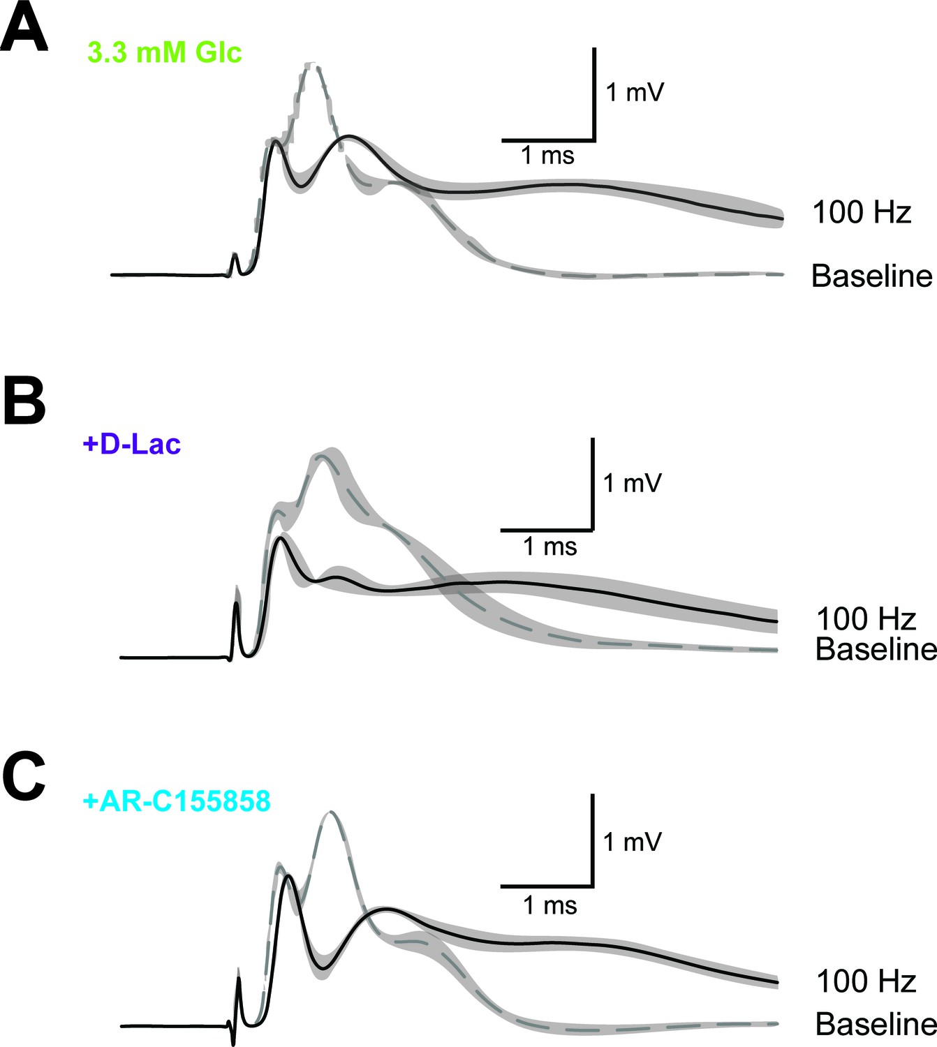
Example of CAP traces before and after high-frequency stimulation (HFS) of optic nerves in the presence of inhibitors of lactate metabolism.
Optic nerves were incubated in aCSF containing 3.3 mM glucose in the absence of inhibitors (A) or in the presence of either 20 mM D-lactate (B) or 10 µM AR-C155858 (C). Shown are mean CAP wave forms (n = 3 nerves for each condition) prior to high- frequency stimulation (‘baseline’; dashed lines) or at the end of the 2.5 min HFS (100 Hz) period (solid lines). Grey areas indicate SEM.
Download links
A two-part list of links to download the article, or parts of the article, in various formats.
Downloads (link to download the article as PDF)
Open citations (links to open the citations from this article in various online reference manager services)
Cite this article (links to download the citations from this article in formats compatible with various reference manager tools)
Monitoring ATP dynamics in electrically active white matter tracts
eLife 6:e24241.
https://doi.org/10.7554/eLife.24241


