Uniting functional network topology and oscillations in the fronto-parietal single unit network of behaving primates
- German Primate Center, Germany
- Georg-August University Göttingen, Germany
Figures
Figure 1 with 1 supplement
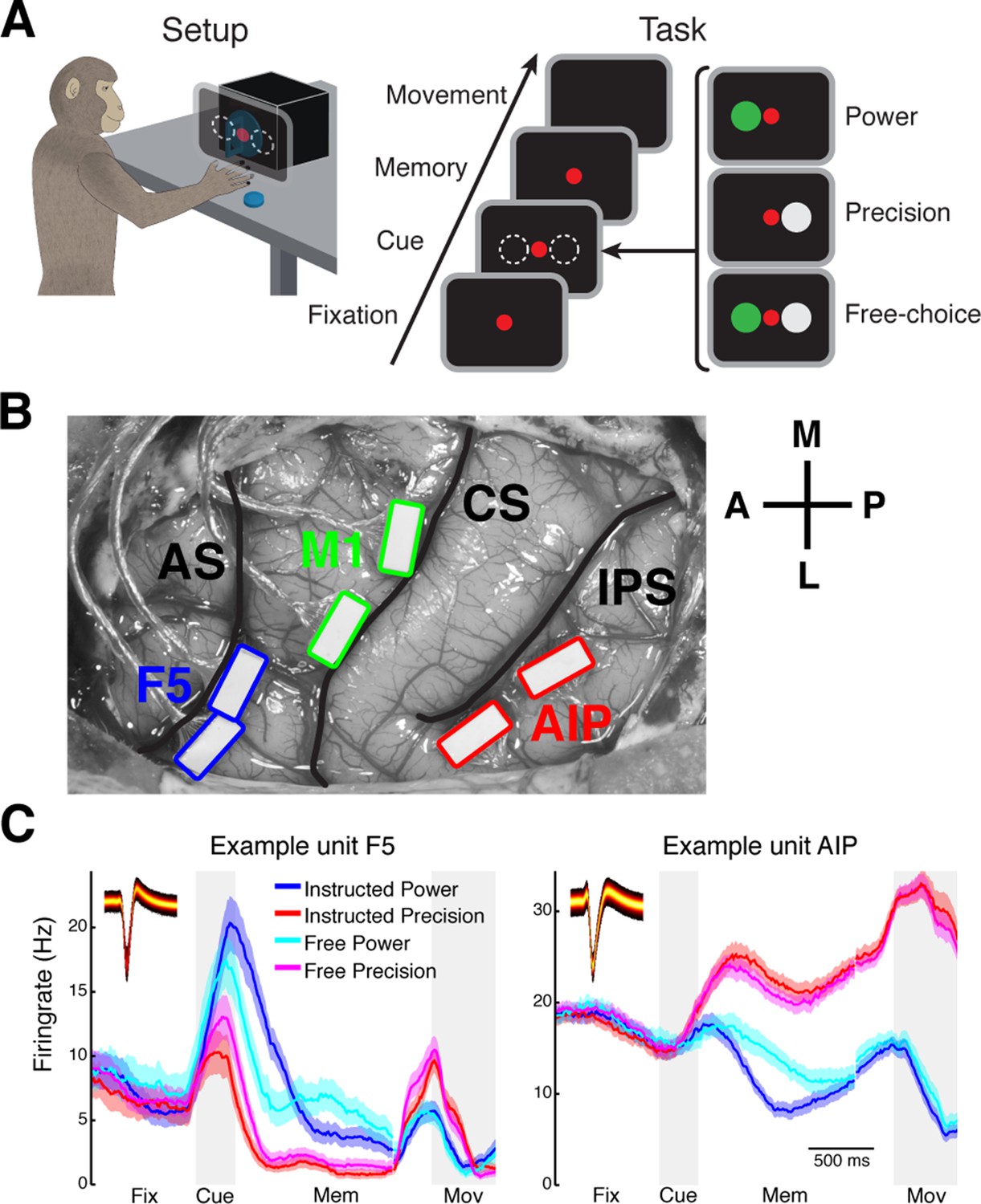
Task design and array implantation.
(A) Choice/no-choice task. Setup: Monkeys were cued to grasp a target (handle) with one of two different grip types displayed on a monitor appearing superimposed on the handle. Task: Monkeys had to fixate a red disk for 600–1000 ms (Fixation), followed by a cue period of 300 ms (Cue). Then, either (‘Power’) a green disk was presented on the left indicating a power grip, (‘Precision’) a grey disk on the right indicating precision grip, or (‘Free-choice’) both disks were presented indicating a free-choice between both grips. After the cue a memory period followed (duration: 1100–1500 ms) before the fixation dot was turned off (go-signal) indicating the monkey to execute the grasp movement (maximum duration:1000 ms). (B) Electrode array implantation of monkey M with 6 floating microelectrode arrays (FMAs) in areas AIP, F5, and M1. Arrays were implanted at the lateral end of the intraparietal sulcus (IPS) in AIP, in the posterior bank of the arcuate sulcus (AS) in area F5, and in the anterior bank of the central sulcus (CS) in the hand area of M1. (C) Average firing rate across trials of two example units from area F5 (left) and AIP (right). Each colored line corresponds to the mean activity of one condition. Line shadings represent standard error. Inlays shows the corresponding waveforms displayed as density plots.
Figure 1—figure supplement 1
Firing rate distribution and stability across task epochs and conditions.
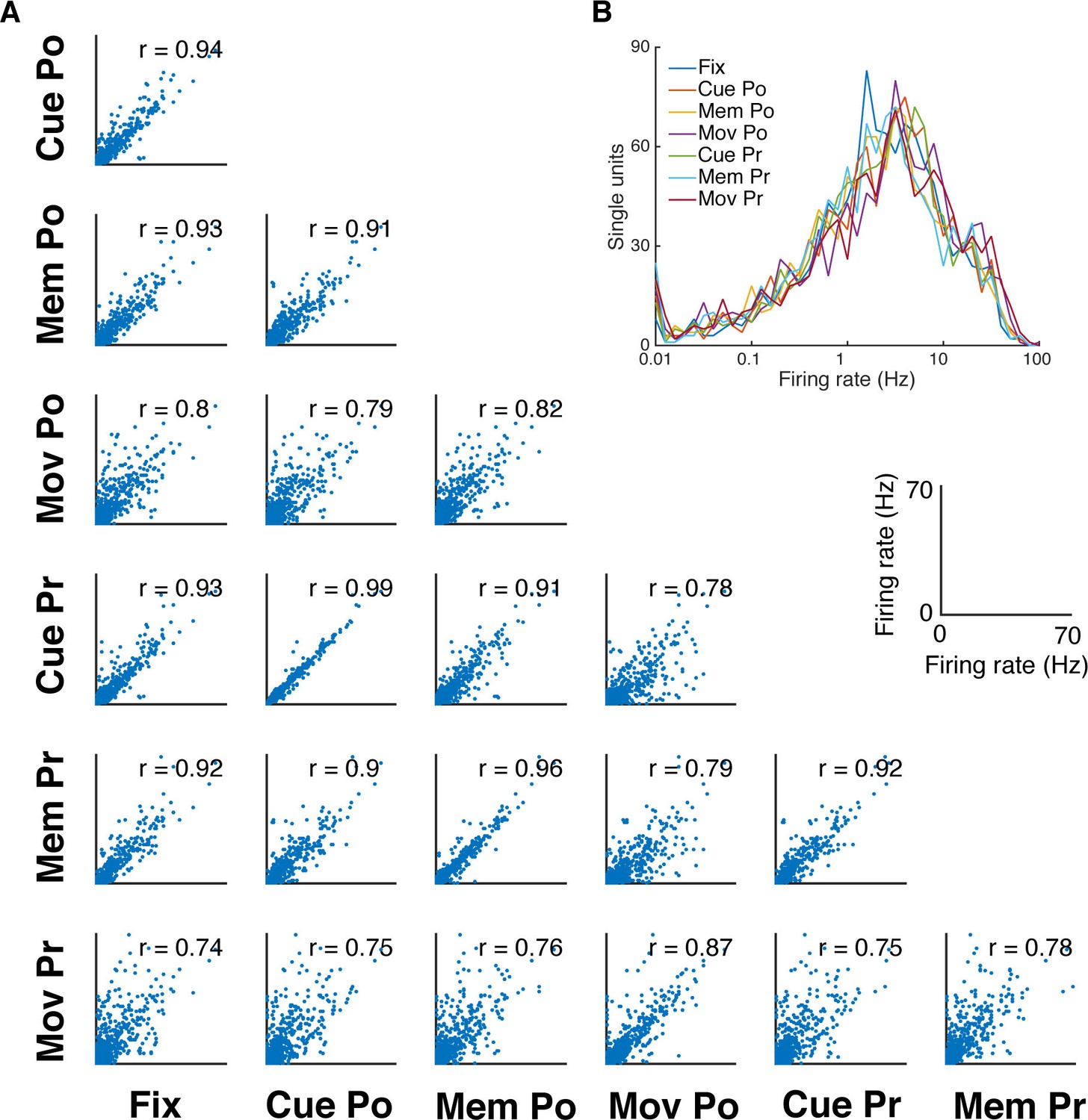
(A) Scatter plots of all pairs of condition- and epoch-wise average firing rates of all recorded single units of all datasets (fixation (Fix), cue power (Cue Po), memory power (Mem Po), movement power (Mov Po), cue precision (Cue Pr), memory precision (Mem Pr) and movement precision [Mov Pr]). Due to the high degree of similarity, free-choice and instructed trials were collapsed. In each panel the corresponding correlation coefficient is displayed (mean r = 0.85, SD = 0.08; for all: p<0.001). (B) Firing rate distribution averaged as in A, displayed on a logarithmic x-axis. The firing rate distribution is very similar for all conditions and epochs and close to log-normal.
Figure 2 with 4 supplements

Cross- and auto-correlation histograms and frequency spectra.
(A) Example crosscorrelation histograms (CCHs) for five example neuron pairs. Displayed amplitude is limited to ±2.5x10⁻³ coincidences per spike for better comparison. CCHs are color-coded based on their oscillatory synchronization frequency (red: beta band; blue: low frequencies; magenta: beta and low frequencies; black: no underlying frequency). (B) Corresponding frequency spectra of CCHs in a, frequency displayed on logarithmic scale (for better comparison limited to a power of 8x10⁻⁵) and color-coded as in A. (C) Same as in A, but for auto-correlation histograms (ACHs). (D) Same as in B, but for the frequency spectra of the ACHs in C. (E) Illustration of different kinds of CCHs to a reference unit and the inferred connectivity. Upper left: No peak is present in the CCH so the unit is not connected to the reference unit. Upper right: A peak at positive time lags indicates a connection from the reference to the target unit. Lower right: A peak is present straddling the 0 time lag with a maximum peak at 0, indicating a bidirectional connection. Lower left: Several peaks and troughs are present with a clear underlying frequency and a maximum peak at a negative time lag, indicating an oscillatory connection from the target to the reference unit.
Figure 2—figure supplement 1

CCH processing and statistics, and all connections of an example unit oscillatory synchronized in the low frequency range.
(A) Processing steps of three example CCHs. From left to right: illustration of the processing steps involving surrogate subtraction, smoothing, and cluster statistics to evaluate if a peak or trough in a CCHs was significant. From top to bottom: A CCH with one significant peak, a CCH with multiple significant peaks and troughs having an underlying frequency in the beta range, and a CCH with no significant peak or trough. (B) An examples of all CCHs (small panels) and the ACH of one unit with all other units of one dataset of a unit communicating and oscillating in the low frequency range. The ACH is boldly framed and displayed in red, significant connections are indicated by dark lines in CCHs and not significant connections as transparent lines. Directionality information, which is also derived from the CCHs, is not represented.
Figure 2—figure supplement 2
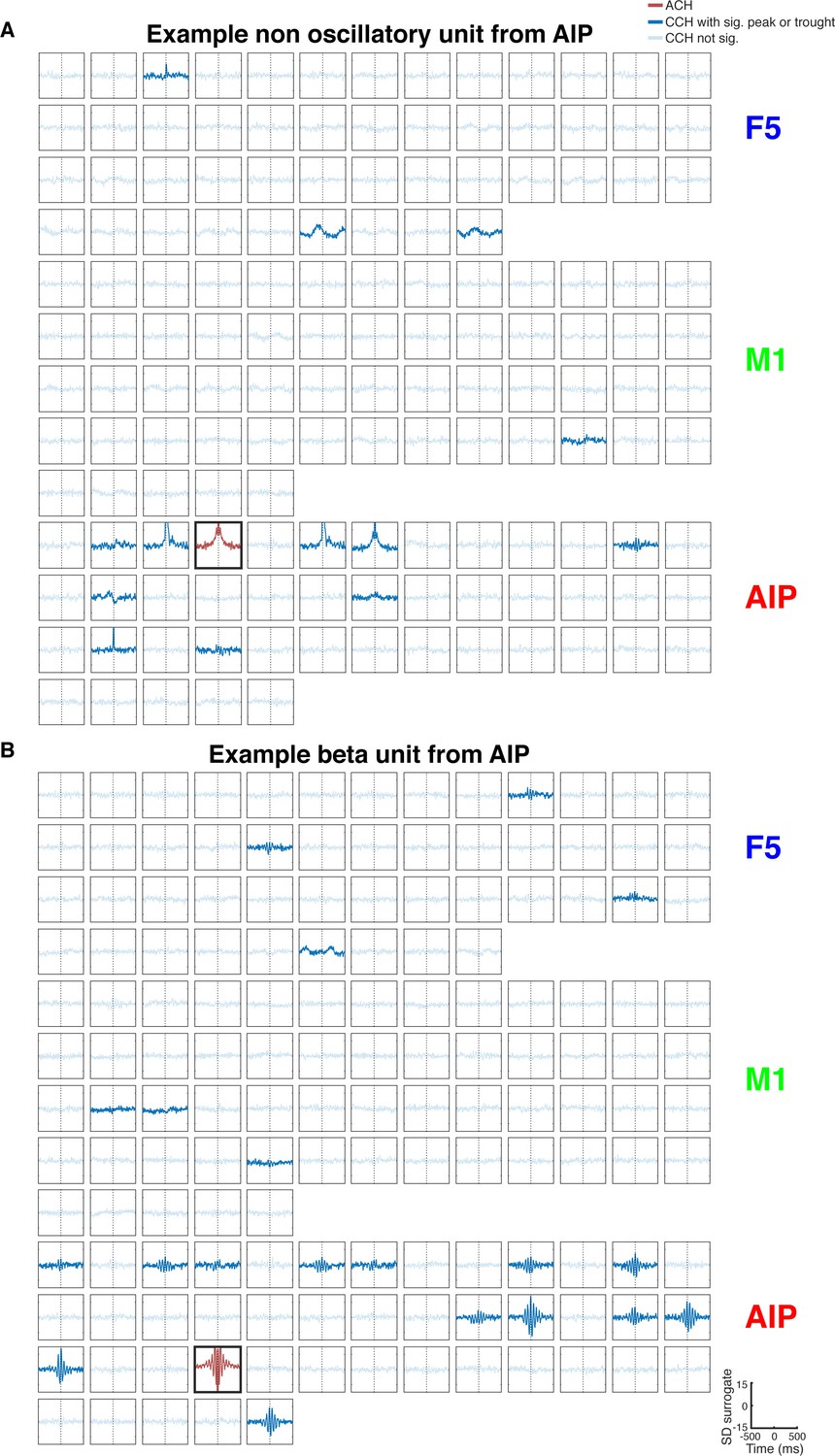
All connections of two example units, one non-oscillatory synchronized and one oscillatory synchronized in the beta range.
(A) Same as in Figure 2—figure supplement1B, but for a non-oscillatory synchronized unit. (B) Same as in Figure 2—figure supplement1B, but for a unit communicating and oscillating in the beta range.
Figure 2—figure supplement 3
Detectability of directed functional connections using equal rate model simulations.
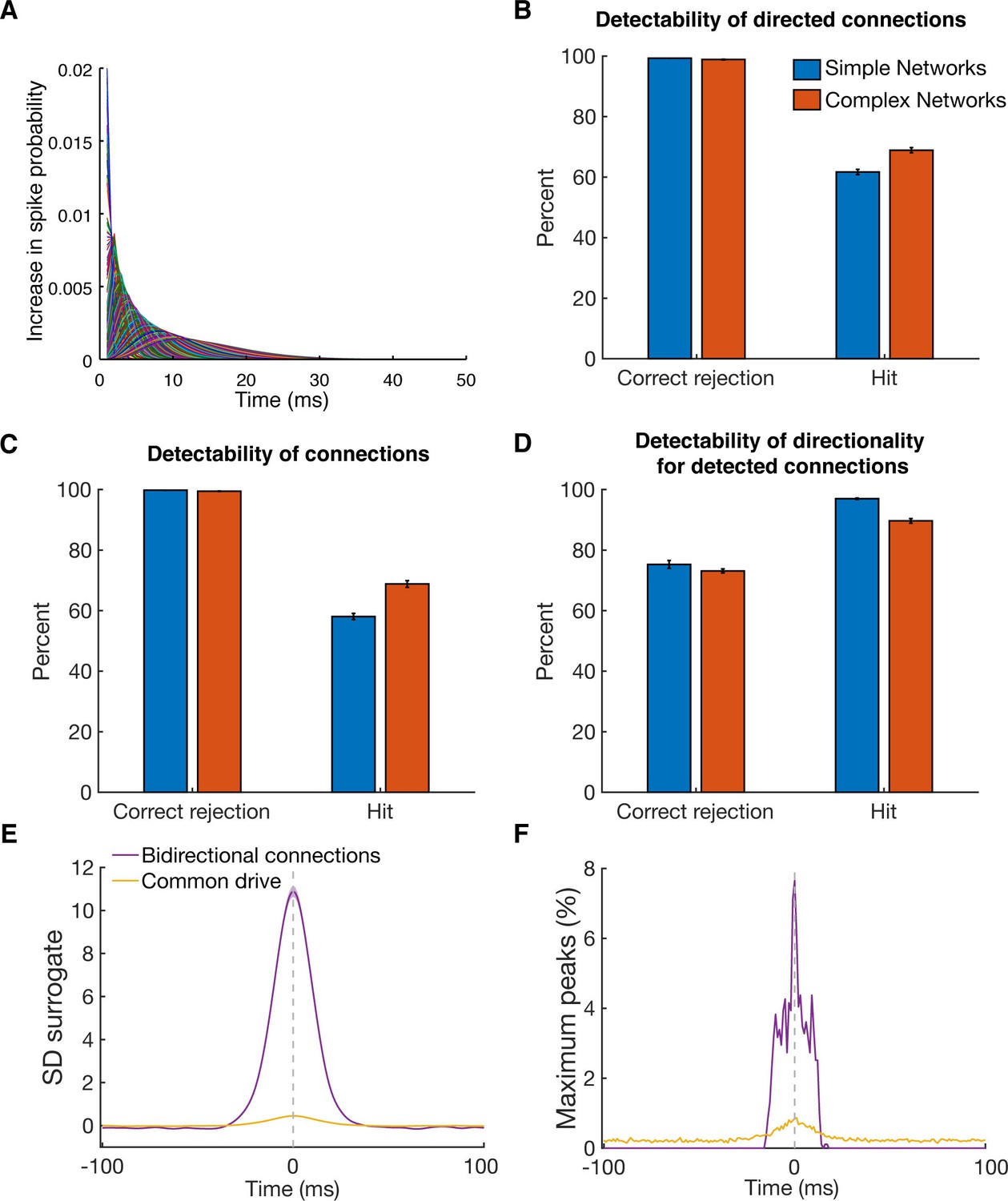
(A) Transfer kernels of one modeled dataset. Gamma functions with different maxima and lengths were used as temporal transfer kernels. The area under the curve was always normalized to 0.02. (B) Histogram of detectability of directed connections. Average number of correct rejections and hits are shown for 10 simulated simple networks (SN) and 10 simulated complex networks. Error bars show the standard error across simulated networks. (C) Same as in B, but for detectability of connections. Any directional information was ignored and it was just estimated if a connection between two units was detected or not. (D) Same as in B, but for detectability of directionality for detected connections. The percent of correct rejections and hits is only for the correctly detected connections as displayed in B, thus a pure evaluation of directionality detectability unbiased by connection detectability. (E) Average CCHs for bidirectional connections and common drive pairs of all 20 simulations. The data was pooled, since no considerable difference between the two types of simulations was found. All simulated pairs of both groups are included irrespective of whether they were detected as significant. Error bars show the standard error across CCHs. Note that even though the average peak is at the zero time lag, many pairs had peaks on either side of the zero time lag. (F) Maximum peak count of bidirectional and common drive pairs (for each ms bin) displayed in E. In case CCHs had two peaks or just showed noise fluctuations, only the time lag of the maximum value was considered in order to avoid preselection biases.
Figure 2—figure supplement 4
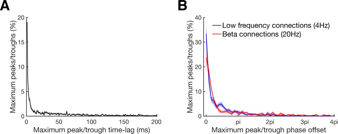
Maximum peak or trough time and phase lag distributions.
(A) Maximum peak or trough time lag distribution of all significant connections relative to the zero time lag. In case that more than one significant cluster was detected, only the cluster with the highest absolute value was considered. For bidirectional connections time lags were considered for both directions. Line shadings show standard error across datasets. (B) Maximum peak or trough phase relative to the zero time lag for all connections with significant underlying oscillation classified by a significant peak in their corresponding frequency spectra. Results are shown separately for beta at 20 Hz (red) and low frequency at 4 Hz (blue) oscillations. Note that 4pi (two cycles) corresponds to 100 ms for beta and to 500 ms for low frequency oscillations. Line shadings show standard error across datasets.
Figure 3 with 2 supplements
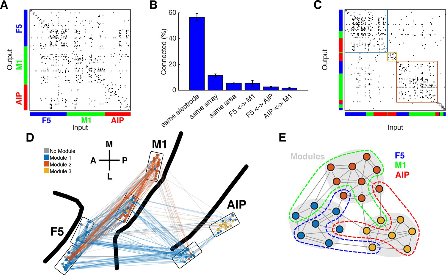
Connectivity characteristics and modular topology.
(A) Connectivity matrix of one dataset from monkey M. Each dot represents a significant connection (Online Methods). Units are ordered by channel number of the recording system. (B) Distance dependent connectivity. From left to right: 56,7%, 11,5%, 5,6%, 5,5%,2,6%, and 1,7%. Note the clear distance dependent decay. (C) The same matrix as in A, but with nodes ordered according to an optimal modularity partition. Colored rectangles surround different network modules. (D) Anatomical network representation of the connectivity matrix in A. The brain is viewed as in Figure 1B. Single units and connections are color coded by module. (E) Schematic illustration of modular topology. Modules (dashed regions) consist mainly of single units of one cortical area, but also include small fractions of units from other areas.
Figure 3—figure supplement 1
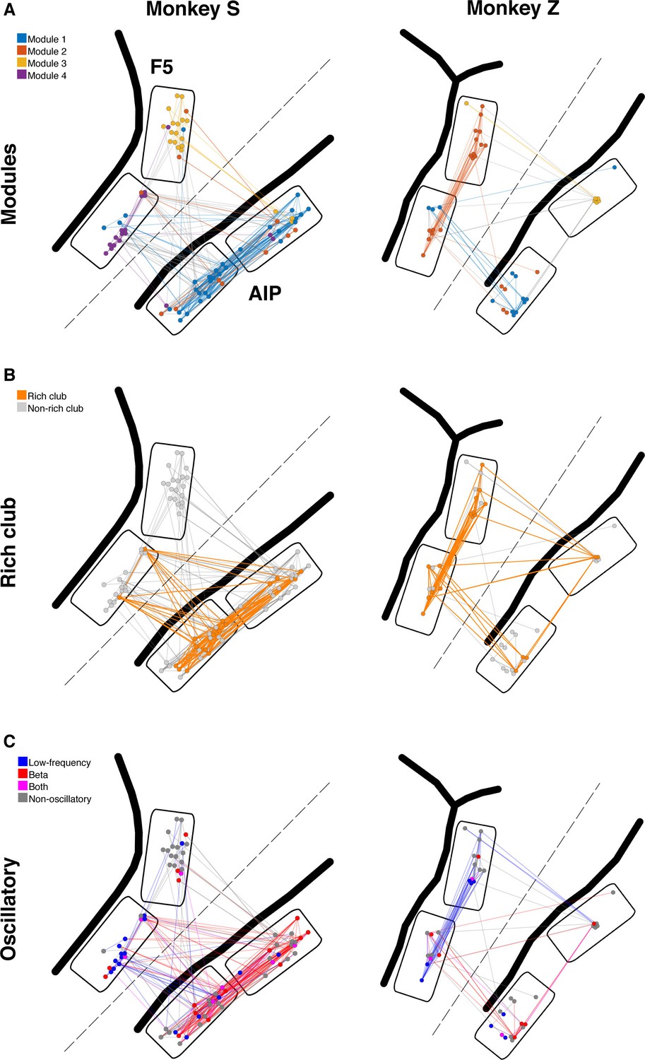
Example anatomical networks from Monkey S and Z.
Since no data were recorded from area M1 for these monkeys, the F5 and AIP arrays are presented closer together than in reality for better illustration (dashed line marks anatomical discontinuity). (A) Each node colored based on the module, as in Figure 3C. (B) Nodes and connections colored based on rich-clubness, as in Figure 4E. (C) Nodes and connections colored based on oscillatory components in the ACHs and CCHs, respectively, as in Figure 5B.
Figure 3—figure supplement 2
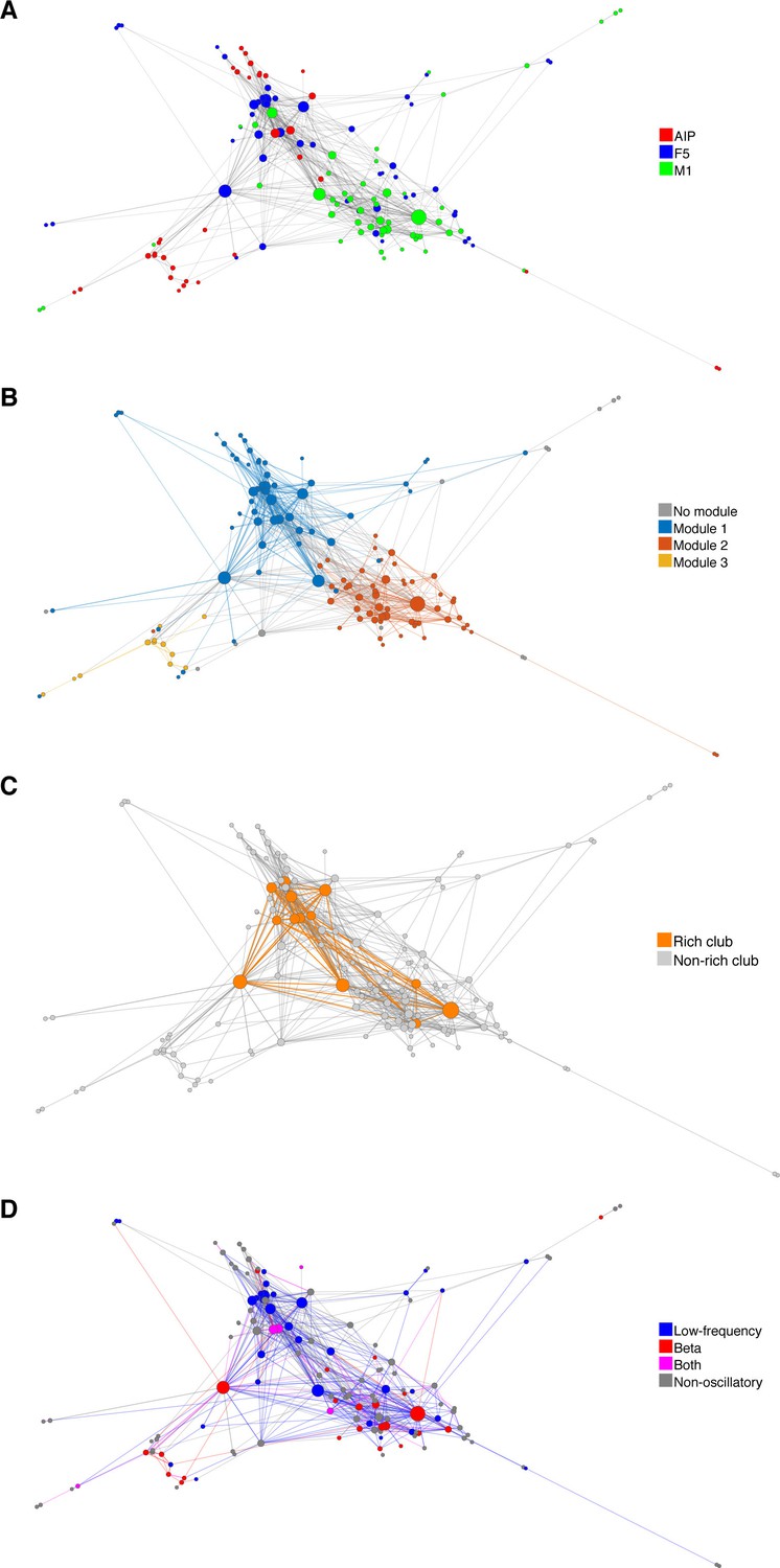
Functional network connectivity of an exemplar data set displayed as a web where the locations of all neurons were determined using the visualization of similarities (VOS) approach (Van Eck and Waltman, 2007).
(A) Each node is colored based on the area it was recorded. (B) Each node colored based on its module. (C) Nodes and connections colored based on oscillatory components in the ACHs and CCHs, respectively. (D) Nodes and connections colored based on rich-clubness. Each circle represents a single neuron and is scaled based on the degree of connectivity. VOS aims to find locations in a low-dimensional space (in this case 2D) in such a way that the distance between each node reflects the similarity between these nodes. Similarity is typically found by calculating the association strength (also known as proximity index) on the co-occurrence matrix of items, which is in this case the weighted network connectivity matrix. Association strength is simply the co-occurrence of two items divided by the product of the number of occurrences of each item. The location of each node is then found by minimizing the sum of the squared distance between all nodes, weighted by the computed similarity between each node. To avoid trivial solutions in which all nodes are assigned the same location, there is an additional constraint that the average distance between all pairs of items must be equal to one. Mathematically, VOS bares much similarity to the method of multi-dimensional scaling (Van Eck et al., 2010). All implementations of VOS were performed using the freely available software, Pajek (http://mrvar.fdv.uni-lj.si/pajek/), and then plotted in Matlab.
Figure 4 with 2 supplements
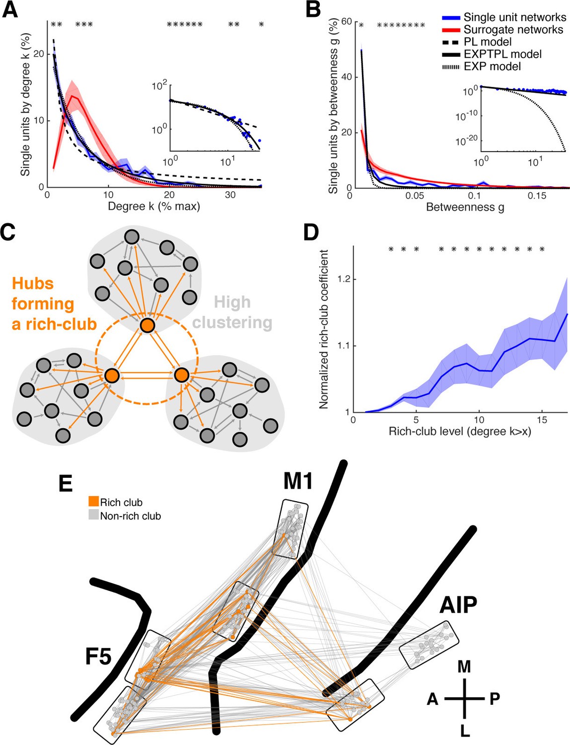
Centrality measures, hubs, and rich-club topology.
(A) Average degree centrality distribution of all networks (blue) and corresponding surrogate networks (red). Black lines reflect different models fitted to the data (see legend in B). The degree distribution of each dataset was normalized to the possible maximum number of connections per network. The area under the curve was normalized to 100% before averaging. Line shadings show standard error across datasets. Asterisks represent significant differences to surrogate networks. Inlay shows the same distribution and models on a log-log scale. (B) Same as in A, but for the betweenness centrality distribution. Note that the slopes for the EXPTPL and PL model are identical, since the exponential coefficient of the EXPTPL model was zero. (C) Schematic view of a rich-club topology connecting highly clustered modules. (D) Average rich-club level of all datasets relative to surrogate datasets. Asterisks represent significant differences of rich-club level to surrogate networks. (E) Anatomical network representation, as in Figure 3D, with connections and units color-coded based on rich-club membership (orange).
Figure 4—figure supplement 1
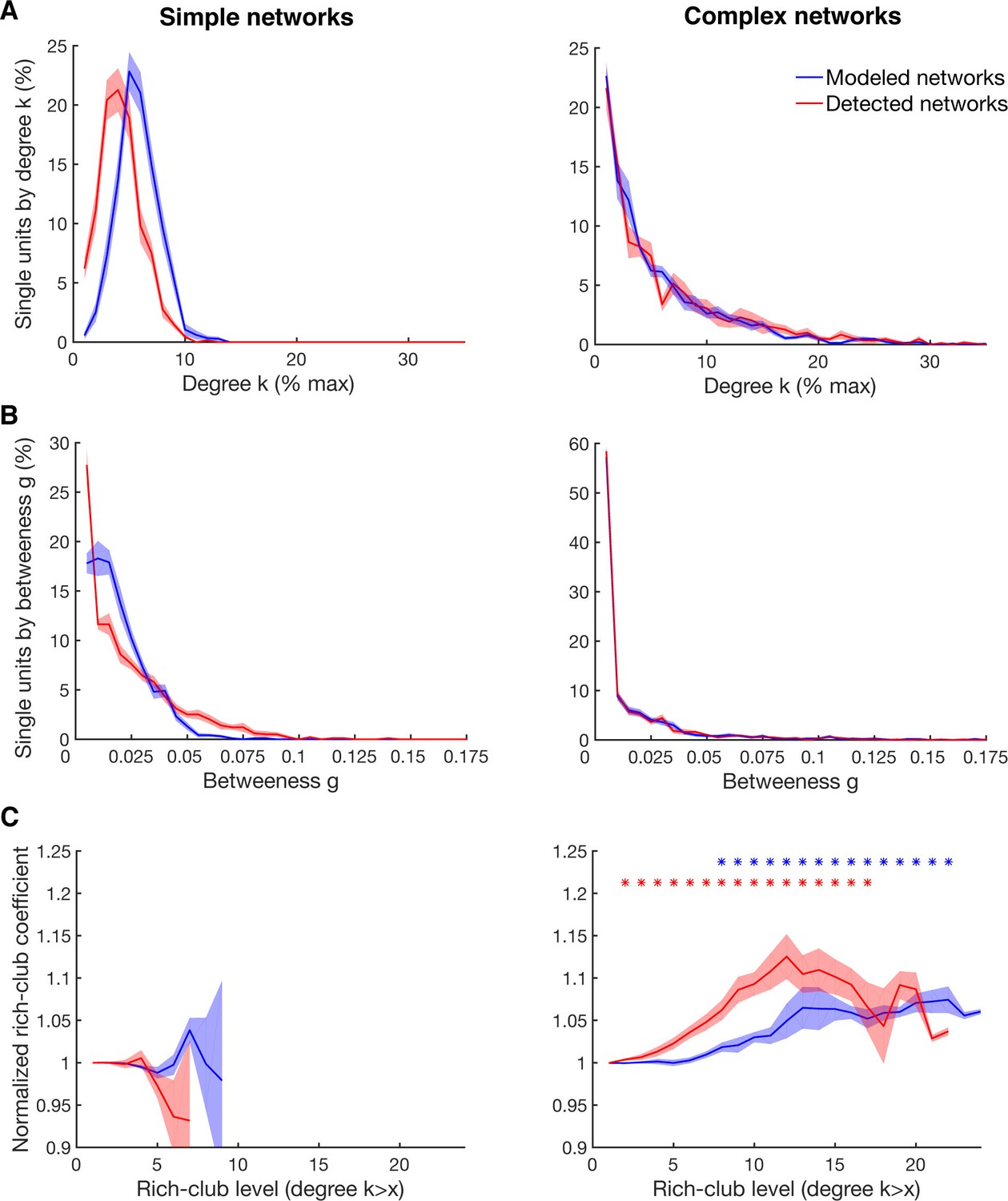
Detectability of the underlying network topology using equal rate model simulations.
(A) Average degree centrality distribution of all networks simulated with the equal rate model (blue) and the corresponding detected networks with the described method for detecting directed functional connectivity (red). Results are shown for the same 10 simulated simple networks and 10 simulated complex networks as in Figure 2—figure supplement 3. Error bars show the standard error across simulated networks. (B) Same as in A, but for the betweenness centrality distributions. (C) Same as in A, but for the rich-club level relative to surrogate datasets. Asterisks represent significant difference of rich-club level to surrogate networks. Two different sets of surrogate networks were calculated per dataset, one for the simulated network and one for the detected network.
Figure 4—figure supplement 2
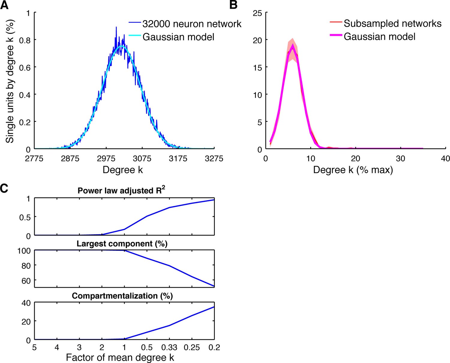
Subsampling model.
(A) Average degree centrality distribution of the modeled neuronal plane (32000 neurons, 2 areas, each divided into 5 subregions coverable by an array, 160 possible electrode position, and a maximum of 20 single units per electrode) with distant dependent random connectivity (Figure 3B). The distribution could be best described by a Gaussian model (adjusted R2 = 0.98). (B) Average degree centrality distribution of 12 different subsamplings of the modeled neuronal plane with exactly the same number of neurons as in the real datasets. Line shadings show standard error across subsamplings. Datasets were processed as in Figure 4A. Average degree distribution could be best described by a Gaussian model (adjusted R2 = 1) and only poorly by a power law model (adjusted R2 = 0.17). (C) Dependency of goodness of power law fit, the size of the largest component relative to the whole network, and the level of compartmentalization on average degree k. Different average degrees were generated by varying the distance-dependent connectivity density of the empirically gained data (Figure 3B) by factors of 1/5, 1/4, 1/3, 1/2, 1, 2, 3, 4, and 5 times to create a neuronal plane. Goodness of power law fit was highly correlated with the size of the largest component (adjusted R2 = 0.93) and the compartmentalization (adjusted R2 = 0.93).
Figure 5 with 3 supplements
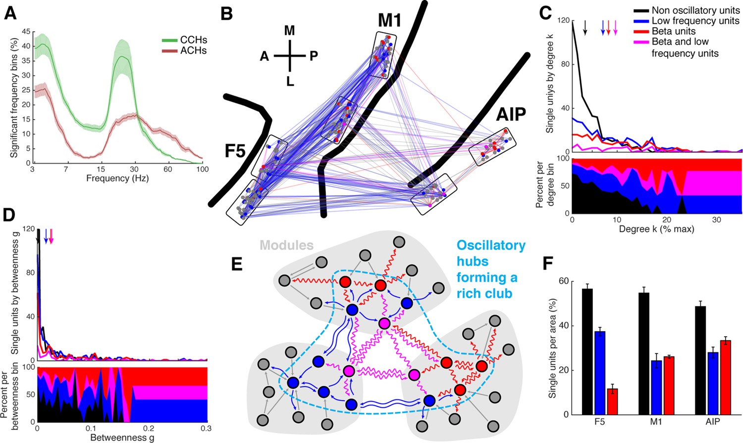
Low frequency and beta oscillators and their network topology.
(A) Average number of significant frequency bins of all ACHs and CCHs over all datasets. Frequencies displayed on a logarithmic scale. Line shadings bars represent standard error across datasets. (B) Anatomical network representation as in Figure 3D with connections and units color-coded by underlying oscillations (see legend in C). (C) Degree centrality distribution of all datasets separately for beta and low frequency oscillators, non-oscillators, and single units oscillating in both frequency ranges. Upper panel, summed degree centrality distribution of all single units. Median degree is represented by arrows in corresponding color: beta units: 7.5, low frequency units: 6.3, beta and low frequency units: 8.9, and for non-oscillators: 2.7. (D) Same as in C but for the betweenness centrality distribution. Median for beta units: 0.023, low frequency units: 0.016, beta and low frequency units: 0.026, and for non-oscillators: 0.001. (E) Schematic view of the found network topology of oscillators. Oscillators form a rich-club spanning all areas. (F) Distribution of oscillators across areas. The number of single units is normalized to 100% per area. F5 has significantly less beta (red) and significantly more low frequency oscillators (blue) than M1 and AIP. Note that units oscillating in both frequency ranges are counted in both. Non-oscillators (black) still remain the largest group in all areas.
Figure 5—figure supplement 1

Frequency dependent Hanning windows used for discrete Fourier transform.
(A) Hanning windows used for discrete Fourier transform of all CCHs. All windows were aligned to the zero bin and span four times the frequency of interest period (with a maximum of 1000 ms and a minimum of 150 ms). Frequencies of interest were scaled logarithmically (100 frequencies from 3 to 100 Hz). (B) Hanning windows used for discrete Fourier transform of all ACHs. All windows were aligned to the zero bin and span two times the frequency of interest period (with a maximum of 500 ms and a minimum of 75 ms). (C) Significant frequency bins of power spectra of all ACHs of one example dataset per monkey. Frequencies were calculated and displayed on a logarithmic scale. (D) Significant frequency bins of power spectra of all CCHs of the same example datasets as in C. (E) Average number of significant frequency bins of all ACHs and CCHs of the same example datasets as in C and D.
Figure 5—figure supplement 2
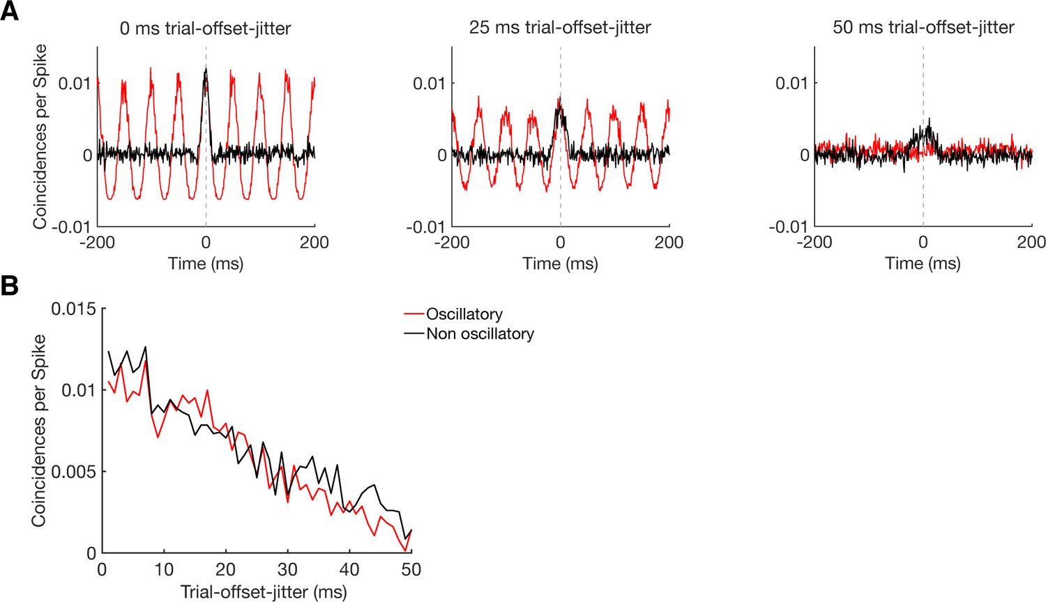
Sensitivity of CCHs in detecting oscillatory synchrony and non-oscillatory synchrony.
(A) CCHs for pairs of simulated neurons with an average firing rate around 5 Hz, either firing in an oscillatory (20 Hz, red curve) or non-oscillatory manner (black curve). By jittering their trial-wise temporal offset in firing, we simulated different levels of coupling strength, without disturbing the firing pattern of the individual neurons nor the similarity in firing between the two neurons. Results are shown for a trial-wise jitter of 0 ms (perfect synchronization), 25 ms, and 50 ms (hardly synchronized). (B) Maximum CCH peak heights of oscillatory and non-oscillatory neurons with a systematical trial-offset-jitter from 0 to 50 ms.
Figure 5—figure supplement 3
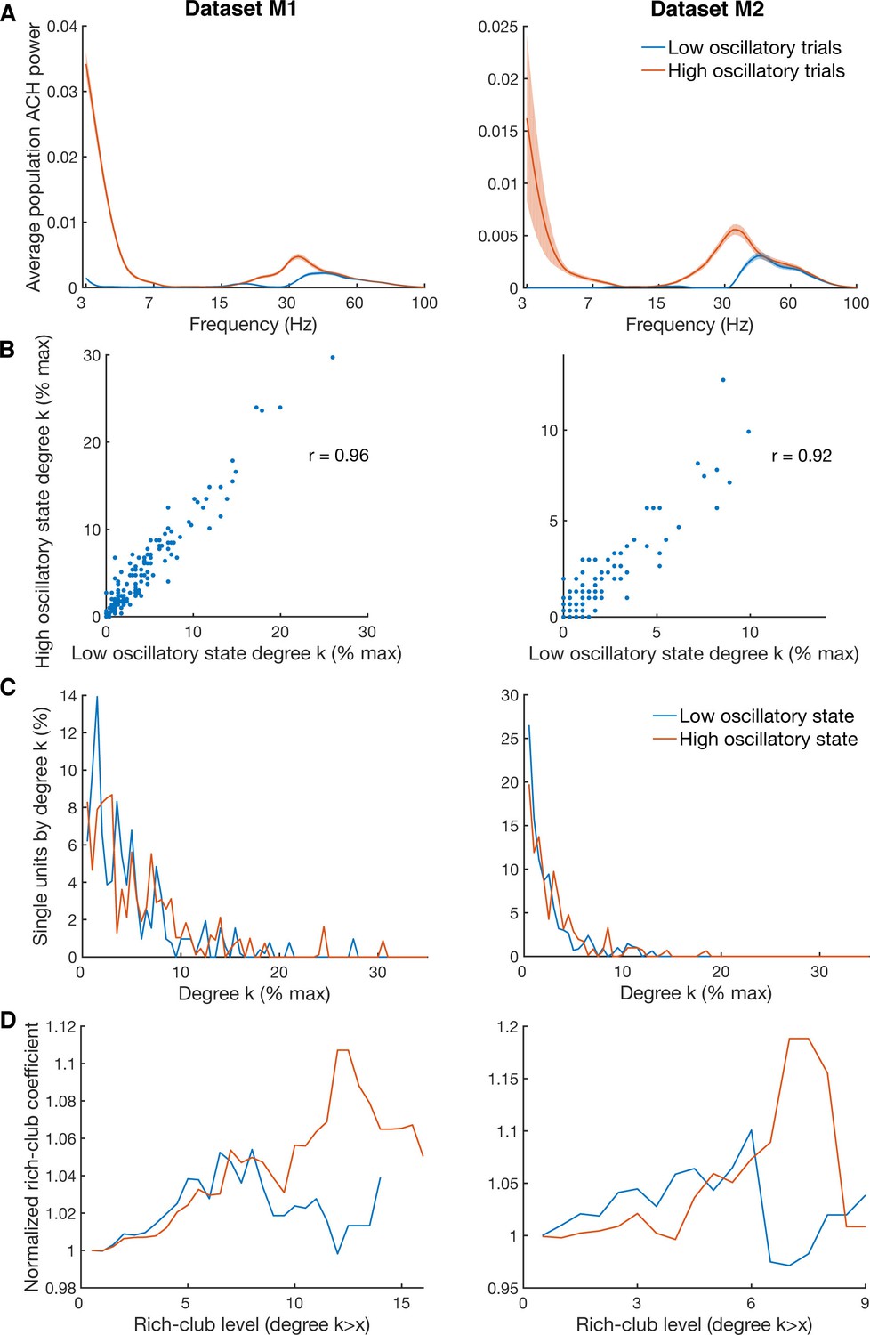
Differences in degree centrality and rich-club level for high and low oscillatory state.
(A) Average power spectra of population ACHs of trials with high power in both the beta (18–35 Hz) and low frequency (3–7 Hz) band (red curve), and of trials with low power in both frequency bands (blue curve). Due to a limited amount of available trials, data is shown only for the two datasets (M1 and M2) with more than 900 trials recorded. (B) Unit-wise degree centrality similarity for networks calculated on low and high oscillatory trials. Degree centrality is normalized by the maximum possible number of connections of all neurons detected. (C) Average degree centrality distribution of the same networks as in B. Degree centrality is normalized by the maximum possible number of connections of all neurons which were interconnected, excluding isolated neurons. Note that this normalization is slightly different between the high and low oscillatory state network and slightly different to B. (D) Same as in C, but for the average rich-club coefficient relative to surrogate datasets.
Figure 6
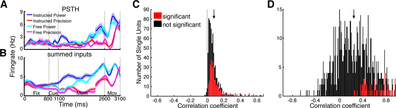
Prediction of firing rates based on network topology.
(A) Average firing rate of one example single unit recorded in F5 in monkey S for the four conditions used in this study during the fixation (Fix), cue (Cue), memory (Mem), and movement period (Mov). The complex tuning patterns for the different task conditions (grip types; free-choice vs. instructed trials) are clearly visible. (B) Predicted firing rate of the same unit as in A based on the population activity of the connected neurons. Curves in (A–B) were smoothed with an additional Gaussian kernel (SD: 40 ms). (C) Histogram of correlation coefficients between the true and predicted spike trains of all single units of all datasets. Significant correlations are marked in red. Note that hardly any correlation coefficient were negative. (D) Histogram of correlation coefficients of condition averaged firing rates. Coloring as in C.
Tables
Table 1
Trial and single unit counts for all datasets. Marked datasets correspond to the displayed example networks in Figures 3–5 and Figure 3—figure supplements 1 and 2. Columns 3–6 show the total and area specific number of units recorded. Columns 7–10 show total and area specific number of units of the largest component of the network, which is the basis for all topological analysis.
| Datasets | Trials | Single units total | F5 | M1 | AIP | Single units used | F5 | M1 | AIP |
|---|---|---|---|---|---|---|---|---|---|
| M 1 | 958 | 149 | 48 | 57 | 44 | 148 | 48 | 57 | 43 |
| M 2 * | 900 | 147 | 52 | 58 | 37 | 137 | 50 | 52 | 35 |
| M 3 | 621 | 107 | 49 | 32 | 26 | 79 | 41 | 20 | 18 |
| S 1 | 503 | 86 | 46 | - | 40 | 57 | 28 | - | 29 |
| S 2 | 565 | 76 | 39 | - | 37 | 64 | 30 | - | 34 |
| S 3 | 460 | 76 | 35 | - | 41 | 64 | 28 | - | 36 |
| S 4 | 460 | 82 | 35 | - | 47 | 64 | 26 | - | 38 |
| S 5 * | 557 | 90 | 42 | - | 48 | 78 | 37 | - | 41 |
| S 6 | 374 | 83 | 42 | - | 41 | 47 | 25 | - | 22 |
| Z 1 | 400 | 52 | 29 | - | 23 | 33 | 21 | - | 12 |
| Z 2 | 436 | 48 | 24 | - | 24 | 30 | 17 | - | 13 |
| Z 3 * | 608 | 59 | 30 | - | 29 | 41 | 21 | - | 20 |
| Average | 570.2 | 87.9 | 39.3 | 49 | 36.4 | 70.2 | 31 | 43 | 28.4 |
| SD | 177.4 | 31.2 | 8.5 | 12.0 | 8.5 | 35.8 | 10.3 | 16.4 | 10.5 |
Table 2
Number of oscillators in all networks analyzed. Marked datasets correspond to the displayed example networks in Figure 5 and Figure 3—figure supplements 1 and 2.
| Datasets | Oscillators total | Non-Oscillators | Beta Oscillators | Low Frequency oscillators | Oscillators in both frequency ranges |
|---|---|---|---|---|---|
| M 1 | 83 | 65 | 37 | 60 | 14 |
| M 2 * | 60 | 77 | 28 | 37 | 5 |
| M 3 | 34 | 45 | 12 | 25 | 3 |
| S 1 | 31 | 26 | 14 | 26 | 9 |
| S 2 | 32 | 32 | 14 | 22 | 4 |
| S 3 | 31 | 33 | 15 | 20 | 4 |
| S 4 | 26 | 38 | 14 | 19 | 7 |
| S 5 * | 40 | 38 | 22 | 25 | 7 |
| S 6 | 21 | 26 | 14 | 10 | 3 |
| Z 1 | 13 | 20 | 5 | 10 | 2 |
| Z 2 | 13 | 17 | 6 | 9 | 2 |
| Z 3 * | 18 | 23 | 10 | 11 | 3 |
| Average | 33.5 | 36.7 | 15.9 | 22.8 | 5.3 |
| SD | 19.4 | 17.4 | 8.7 | 13.8 | 3.4 |
Download links
A two-part list of links to download the article, or parts of the article, in various formats.
Downloads (link to download the article as PDF)
Open citations (links to open the citations from this article in various online reference manager services)
Cite this article (links to download the citations from this article in formats compatible with various reference manager tools)
Uniting functional network topology and oscillations in the fronto-parietal single unit network of behaving primates
eLife 5:e15719.
https://doi.org/10.7554/eLife.15719


