GLO-Roots: an imaging platform enabling multidimensional characterization of soil-grown root systems
- Carnegie Institution for Science, United States
- University of Liège, Belgium
- Department of Energy Joint Genome Institute, United States
- Stanford University, United States
- University of California, Davis, United States
- Harvard Medical School, United States
- United States Department of Agriculture, United States
Figures
Figure 1 with 5 supplements
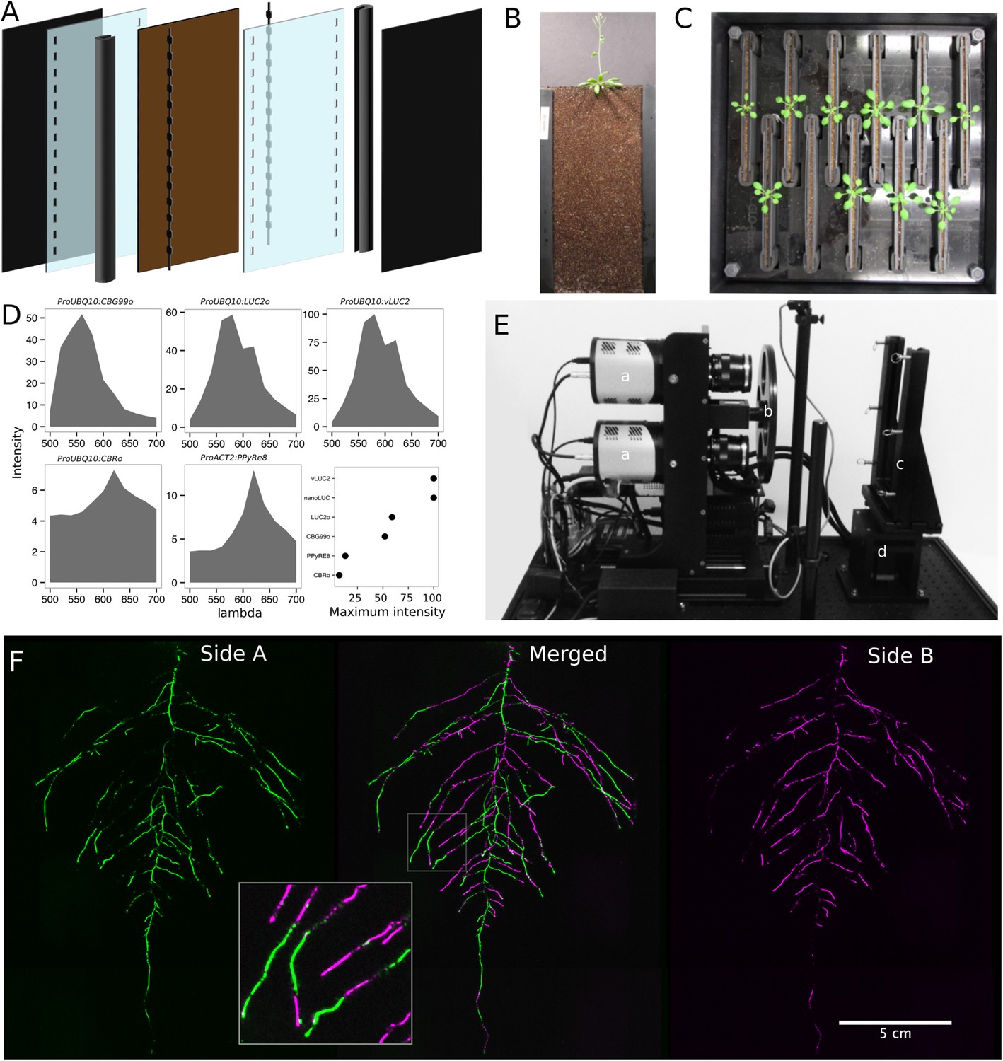
GLO-Roots growth and imaging system.
(A) 3D representation of the different physical components of the rhizotron: plastic covers, polycarbonate sheets, spacers, and rubber U-channels. Blueprints are provided in Supplementary file 1. In brown, soil layer. (B) A 35-day-old plant in rhizotron with black covers removed. (C) Top view of holding box with eleven rhizotrons. (D) In vivo emission spectra of different luciferases used in this study. Transgenic homozygous lines expressing the indicated transgenes were grown on agar media for 8 days. Luciferin (300 μM) was sprayed on the seedlings and plates were kept in the dark and then imaged for 2 s at wavelengths ranging from 500 to 700 nm. Five intensity values were taken from different parts of the roots of different seedlings and averaged. Relative maximum intensity values are indicated in the lower right graph. (E) GLO1 (Growth and Luminescence Observatory 1)-imaging system. The system is composed of two back illuminated CCD cameras (a) cooled down to −55°C. A filter wheel (b) allows for spectral separation of the different luciferases. On the right, a rhizotron holder (c) is used to position the rhizotrons in front of the cameras. A stepper motor (d) rotates the rhizotron 180° to image both sides. (F) A 21 DAS plant expressing ProUBQ10:LUC2o was imaged on each of two sides of the rhizotron; luminescence signal is colorized in green or magenta to indicate side. In the middle of the panel, a combined image of the two sides is shown. The inset shows a magnified part of the root system.
-
Figure 1—source data 1
Two way ANOVA p-values comparing plants grown in MS media vs plants grown in soil (pots or rhizotrons) and plants collected at day or night.
We used p-value < 0.00065 threshold based on Bonferroni adjustment for multiple testing.
- https://doi.org/10.7554/eLife.07597.005
-
Figure 1—source data 2
Luminescence intensity values of the different luciferase isoforms across the emission spectrum.
- https://doi.org/10.7554/eLife.07597.006
-
Figure 1—source data 3
Gene expression values used to construct the PCA of root samples.
Shoot fresh weight (FW), shoot area, lateral root number and primary root length of plants grown in different containers and media.
- https://doi.org/10.7554/eLife.07597.007
-
Figure 1—source data 4
Gene expression values used to construct the PCA of shoot samples.
- https://doi.org/10.7554/eLife.07597.008
-
Figure 1—source data 5
Shoot Fresh Weight (FW) and primary root length of plants grown with or without luciferin.
- https://doi.org/10.7554/eLife.07597.009
-
Figure 1—source data 6
Ground truth and GLO-RIA measured values of directionality, depth and width use for validation.
- https://doi.org/10.7554/eLife.07597.060
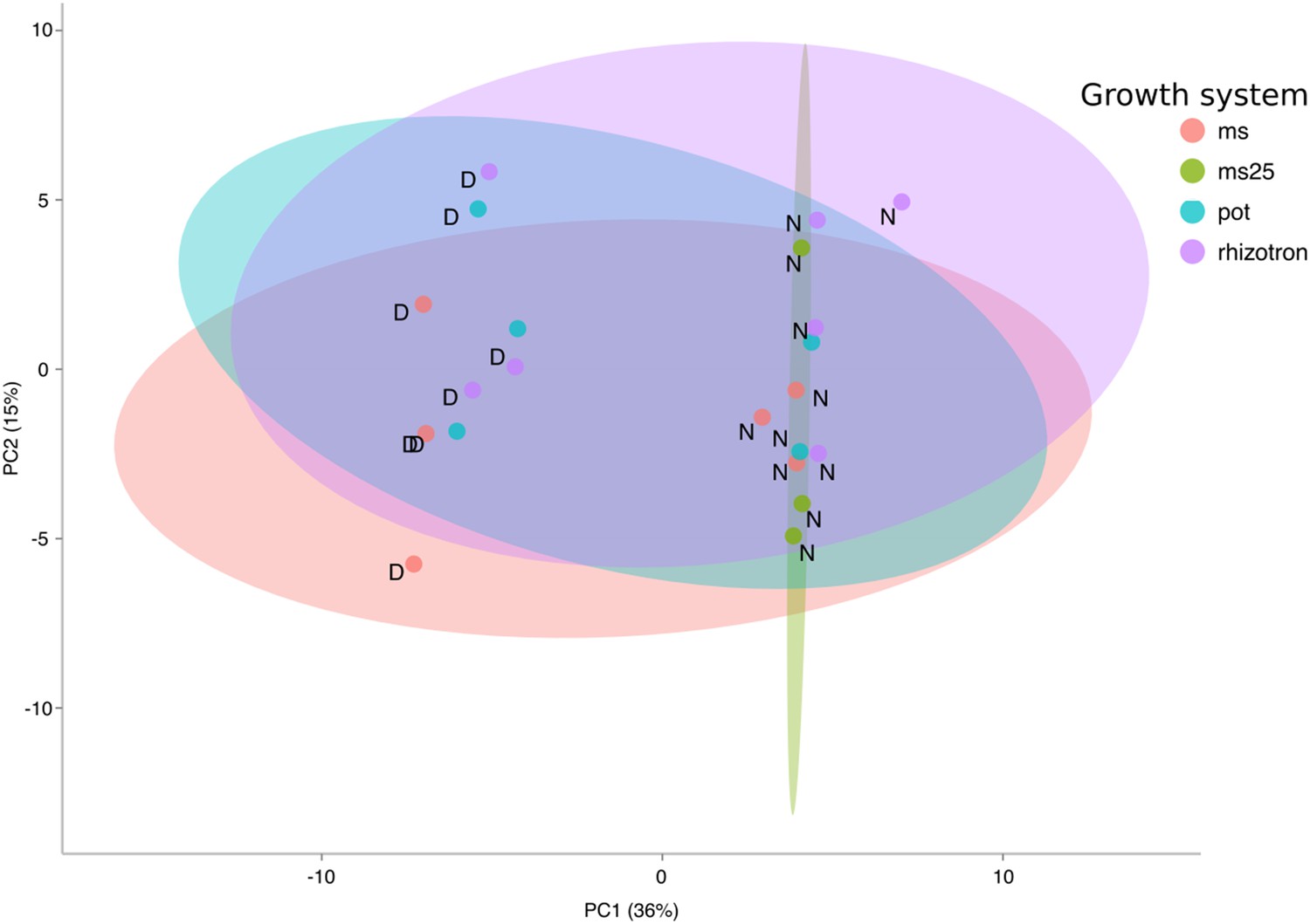
Figure 1—figure supplement 1

Effect of different growth systems on gene expression and growth.
(A) Principal components analysis (PCA) score plot of a set of 76 genes analyzed by qPCR from root samples of plants grown in MS plates, pots, and rhizotrons. After 15 DAS, three plants were collected at the end of the day [D] and three were collected at the end of the night [N]. (ms = plant grown in full ms and 1% sucrose, ms25 = plants grown in 25% of full ms). (B) Leaf area and (C) primary root length of plants of the same age (15 DAS) as the ones used for the qPCR experiment (n = 6–7). (D) Lateral root number and (E) primary root length of 18 DAS plants grown in 30-cm tall cylinders, pots, and rhizotrons, all with a volume of 100 cm3 (n = 6–12 plants). Analysis of Variance (ANOVA) analysis with p < 0.01 was used to test significant differences between the different parameters.
Figure 1—figure supplement 2
PCA plot of shoots of the same samples analyzed in Figure 1.
See Figure 1 for more details regarding experimental conditions used.
Figure 1—figure supplement 3
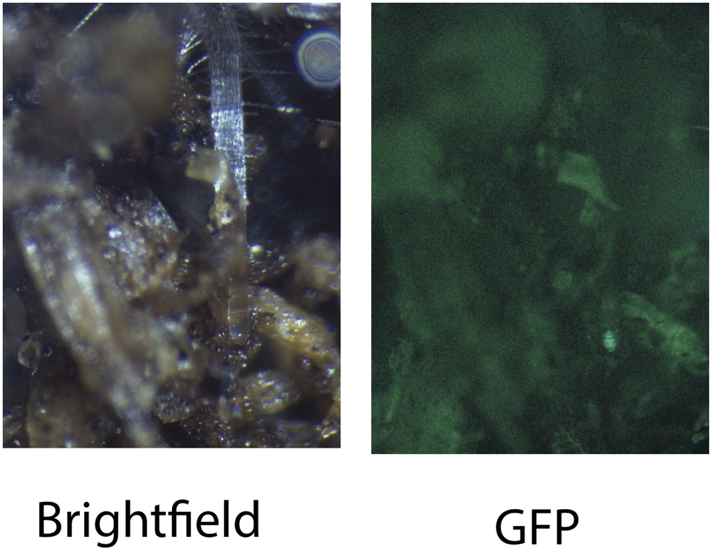
Image of an Arabidopsis root in soil imaged with white light (brightfield) or epifluorescence.
https://doi.org/10.7554/eLife.07597.012
Figure 1—figure supplement 4
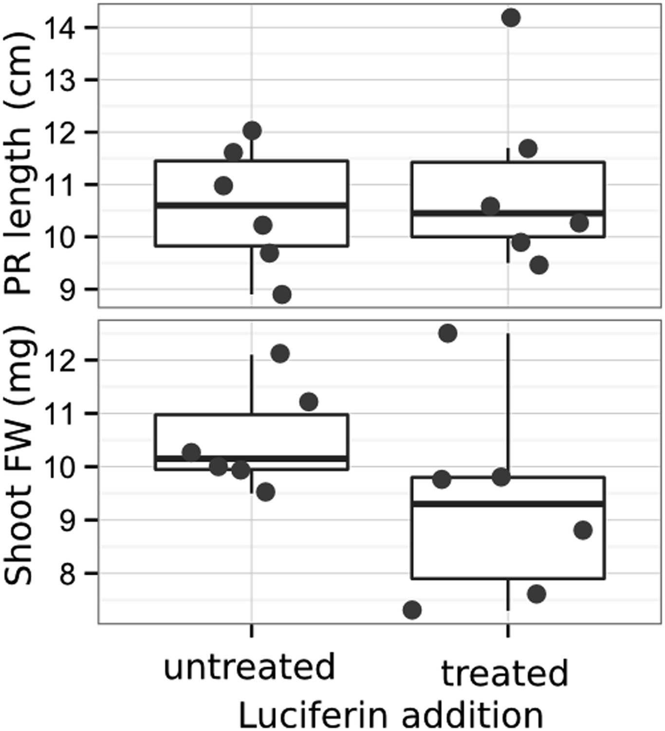
Effect of luciferin addition on primary root length and shoot size of 14 DAS seedlings that were either continuously exposed to 300 μM luciferin from 9 DAS after sowing or not (n = 6-7 plants).
T-test showed no significant differences between treatments at threshold of p < 0.01.
Figure 1—figure supplement 5
GLO-RIA ground truth comparison.
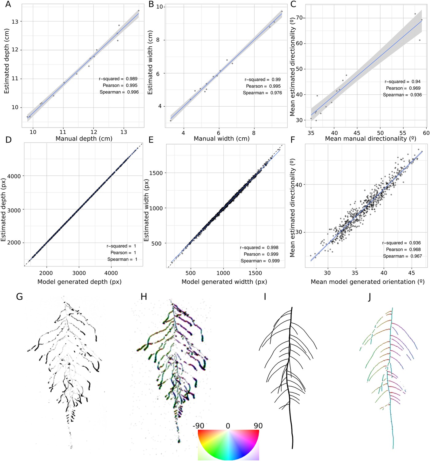
Tests of GLO-RIA were performed using two approaches. We first manually quantified root system depth (A) width (B) and average lateral root angle (C) in a set of 15 root systems corresponding to different Arabidopsis accessions. We also generated 1240 contrasting root systems using ArchiSimple and quantified root system depth, (D) width (E), and directionality (F) using GLO-RIA. Example of a real (G) and ArchiSimple generated (H) root system and corresponding GLO-RIA determined directionality color-coded into the image (I, J). Absolute orientation angle values are taken before all calculations.
Figure 2
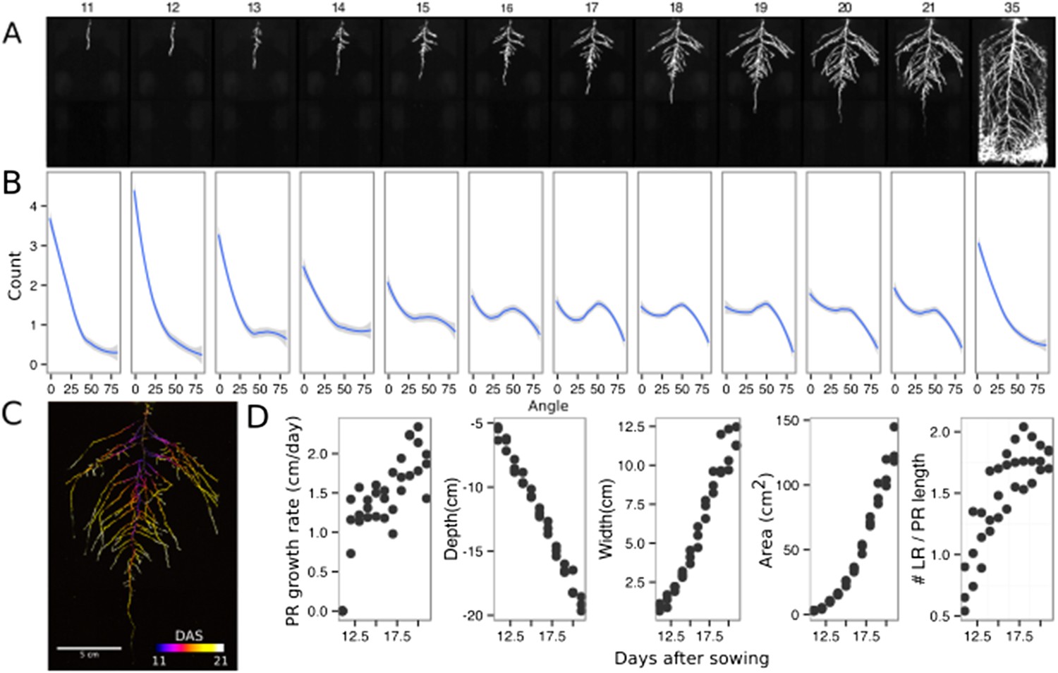
Time-lapse imaging of Arabidopsis root systems and quantification using GLO-RIA.
(A) Typical daily time-lapse image series from 11 to 35 DAS of a ProUBQ10:LUC2o Col-0 plant. (B) Average directionality of three root systems imaged in time series as in panel A calculated using the directionality plugin implemented in GLO-RIA. See the GLO-RIA ‘Materials and methods’ section for information of how the directionality is calculated. (C) Color-coded projection of root growth using the images in panel A. (D) Root system depth, width, root system area are automatically calculated from the convex hull, which is semi-automatically determined with GLO-RIA (n = 3). Primary root length, lateral root number and number of lateral roots divided by the primary root length were quantified manually. A local polynomial regression fitting with 95% confidence interval (gray) was used to represent the directionality distribution curve. 0° is the direction of the gravity vector.
-
Figure 2—source data 1
Directionality and whole root system architecture trait values from the time series.
- https://doi.org/10.7554/eLife.07597.018
Figure 3 with 1 supplement
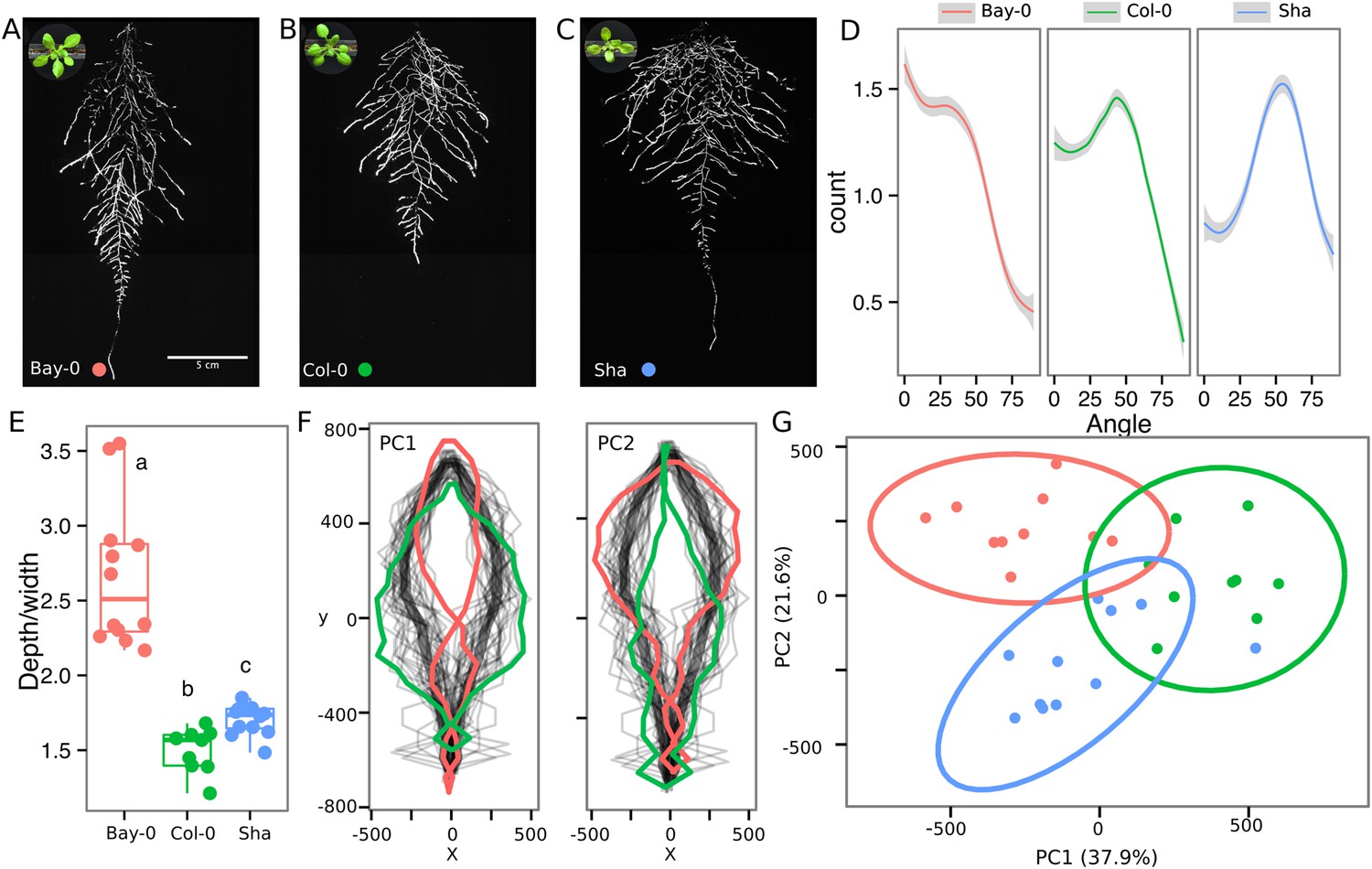
Variation in root architecture between accessions of Arabidopsis.
Representative root and shoot images of (A) Bay-0, (B) Col-0, and (C) Sha accessions transformed with ProUBQ10:LUC2o and imaged after 22 DAS. (D) Directionality of the root systems, (E) depth/width ratio, (F) pseudo-landmarks describing shape variation in root system architecture. Eigenvalues derived from the analysis of 9–12 plants per accession are shown. The first two principal components explaining 38% (PC1) and 22% (PC2) of the shape variation are plotted. PC1 captures homogeneity of root system width along the vertical axis and PC2 a combination of depth and width in top parts of the root system. Red and green lines indicate −3SD and +3SD (Standard Deviations), respectively. (G) PC separation of the different ecotypes using the PCs described in (F). A local polynomial regression fitting with 95% confidence interval (gray) was used to represent the directionality distribution curve. 0° is the direction of the gravity vector. Kolmogorov-Smirnov test at p < 0.001 showed significant differences in directionality distributions between all three accessions. Wilcoxon test analysis with p < 0.01 was used to test significant differences between the different accessions (n = 9–12 plants).
-
Figure 3—source data 1
Directionality, whole root system architectural trait values and shape predictors from Bay-0, Col-0 and Sha.
- https://doi.org/10.7554/eLife.07597.021
-
Figure 3—source data 2
Shape predictor values (TPS format) from Bay-0, Col-0 and Sha used to perform PCA.
- https://doi.org/10.7554/eLife.07597.022
-
Figure 3—source data 3
Whole root system architecture trait values from Bay-0, Col-0 and Sha.
- https://doi.org/10.7554/eLife.07597.023
Figure 3—figure supplement 1

(A) Root area, (B) vertical center of mass of Bay-0, Col-0, and Sha accessions.
Wilcoxon test analysis with p < 0.01 was used to test significant differences between the accessions (n = 9-12 plants).
Figure 4 with 4 supplements
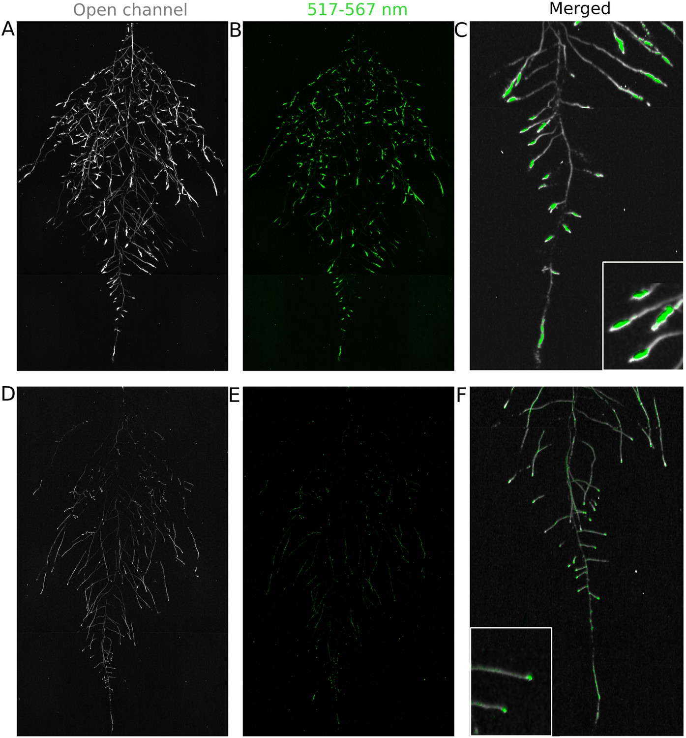
Dual-color reporter visualization of root structure and gene expression.
Images of whole-root systems (A, D) or magnified portion of roots (C, F) at 22 DAS expressing ProACT2:PPYRE8o and ProZAT12:LUC (green, A, B, C) or ProDR5rev:LUC+ (green, D, E, F). Luminescence from PPyRE8 and LUC reporters visualized together using an open filter setting (visualized in grey-scale) while LUC signal is distinguished using a band-pass filter (517 to 567 nm, visualized as green).
-
Figure 4—source data 1
Data for ProZAT12:LUC reporter gene expression in root segments extracted from a whole root system.
- https://doi.org/10.7554/eLife.07597.026
-
Figure 4—source data 2
Luciferase intensity values from the root tip to maturation zone of ProUBQ10:LUC2o, ProZAT12:LUC and ProDR5:LUC+.
- https://doi.org/10.7554/eLife.07597.027
-
Figure 4—source data 3
Distances to boundary between plants.
Shoot FW, root system architecture and shoot area of single and pairs of plants grown in the same rhizotron.
- https://doi.org/10.7554/eLife.07597.028
Figure 4—figure supplement 1
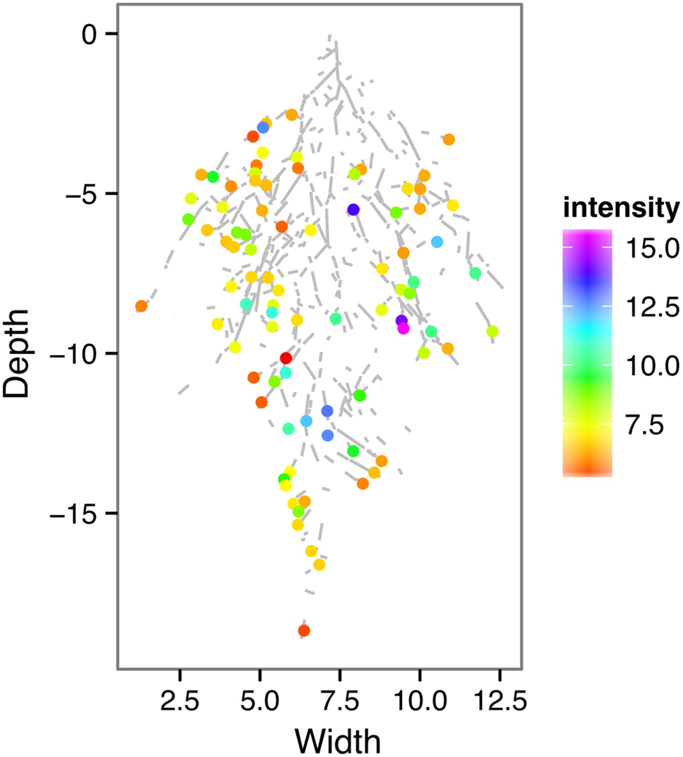
ProZAT12:LUC intensity and root segments automatically identified with GLO-RIA.
https://doi.org/10.7554/eLife.07597.029
Figure 4—figure supplement 2
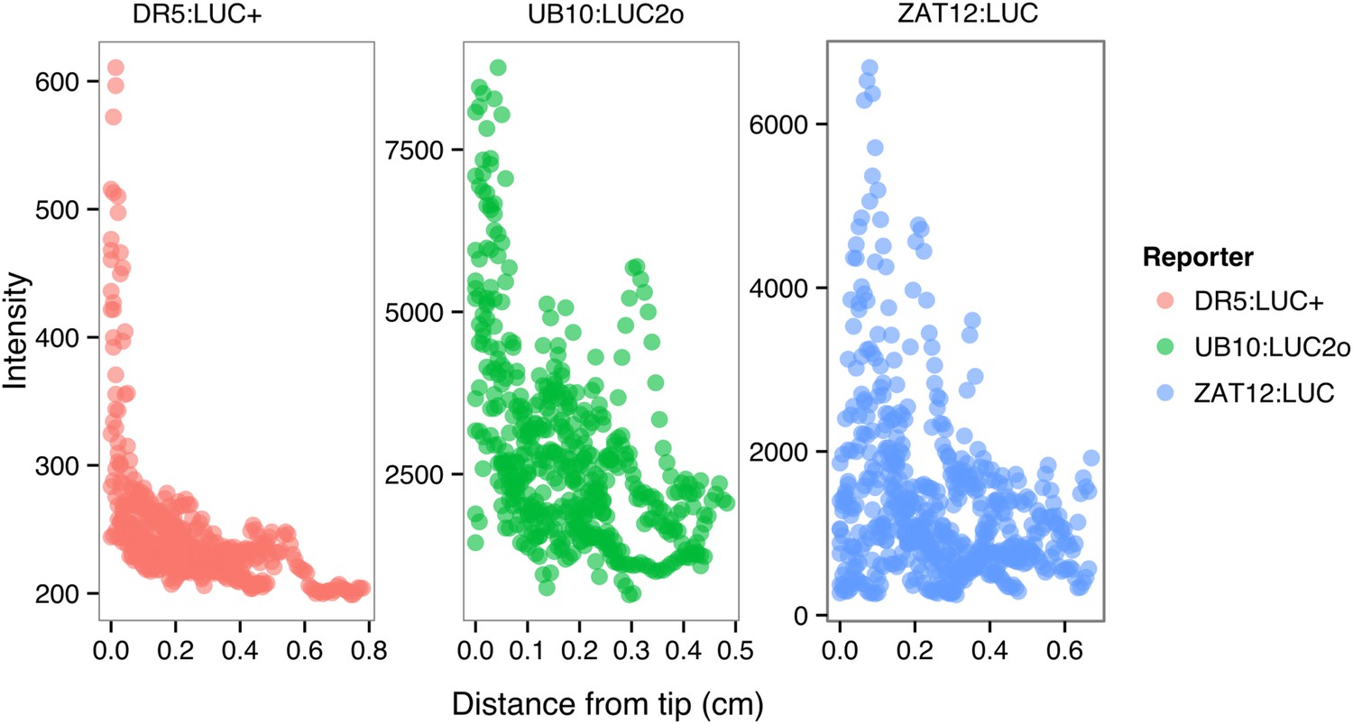
ProDR5rev:LUC+, ProUBQ10:LUC2o, and ProZAT12:LUC intensity values along the root tip.
Data were manually obtained by measuring the intensity profile of the first 0.5 cm from the root tip of individual lateral roots. 10 lateral roots for each reporter were measured.
Figure 4—figure supplement 3
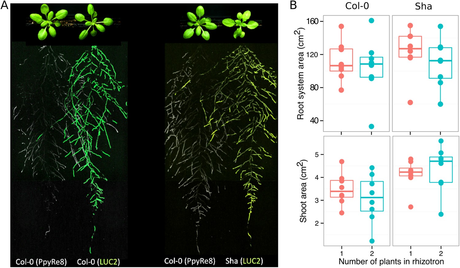
Images of plants at 22 DAS growing in the same rhizotron and expressing different luciferases.
(A) Two Col-0 plants expressing ProUBQ10:LUC2o and ProACT2:PPyRE8o (B) Col-0 plant expressing ProACT2:PPyRE8o and Sha plant expressing ProUBQ10:LUC2o. Wilcoxon test analysis with p < 0.01 showed no significant differences between treatments (n = 7-8 plants).
Figure 4—figure supplement 4
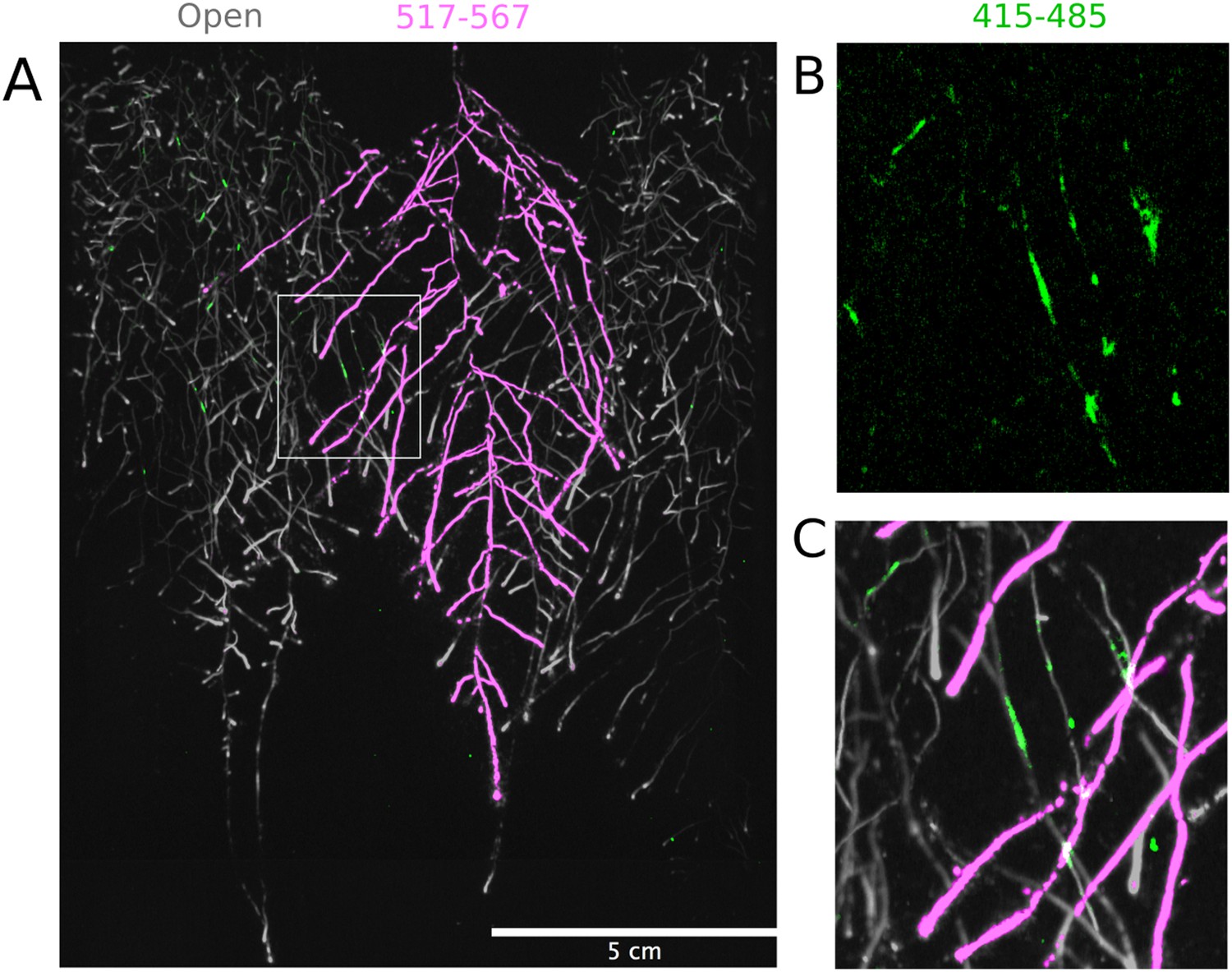
Three reporter-based analysis of root–root–microbe interactions.
(A) Image showing a 22 DAS ProUBQ10:LUC2o plant (magenta) grown in the same rhizotron with ProACT2:PpyRE8o plants (gray). Plants were inoculated with Pseudomonas fluorescens CH267 (green). Magnified portion of root systems colonized by P. fluorescens showing P. fluorescences (B) only or all three reporters together (C).
Figure 5 with 2 supplements
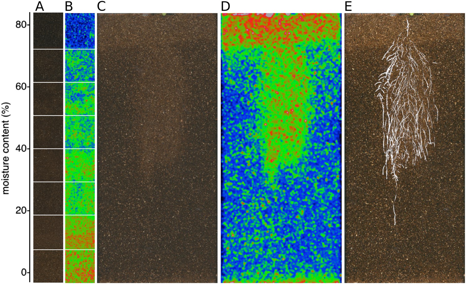
Soil moisture and root architecture mapping in rhizotrons.
(A) Composite image showing regions of soil taken from rhizotrons prepared with different moisture levels. (B) Differences in gray-scale intensity values were enhanced using a 16-color look-up table (LUT). Brightfield image of soil in rhizotron (C) and converted using 16-color LUT to enhance visualization of distribution of moisture (D). (E) Root system of a Bay-0 22 DAS subjected to WD since 13 DAS. Root system visualized using luminescence and overlaid on brightfield image of soil in (C).
-
Figure 5—source data 1
Pixel intensity and water content values used to construct calibration curve.
- https://doi.org/10.7554/eLife.07597.034
Figure 5—figure supplement 1
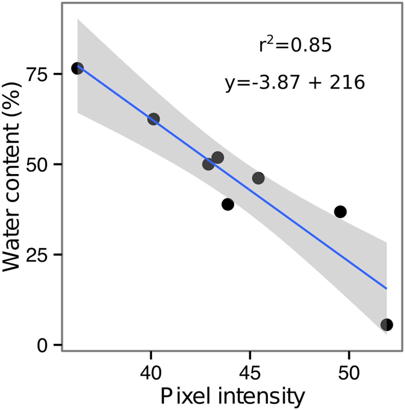
Moisture calibration curve.
Rhizotrons with different levels of moisture were prepared and scanned to obtain readings of pixel intensity. Soil from rhizotrons was then weighed, dried down in an oven at 70°C for 48 hr, and percent water content quantified.
Figure 5—figure supplement 2
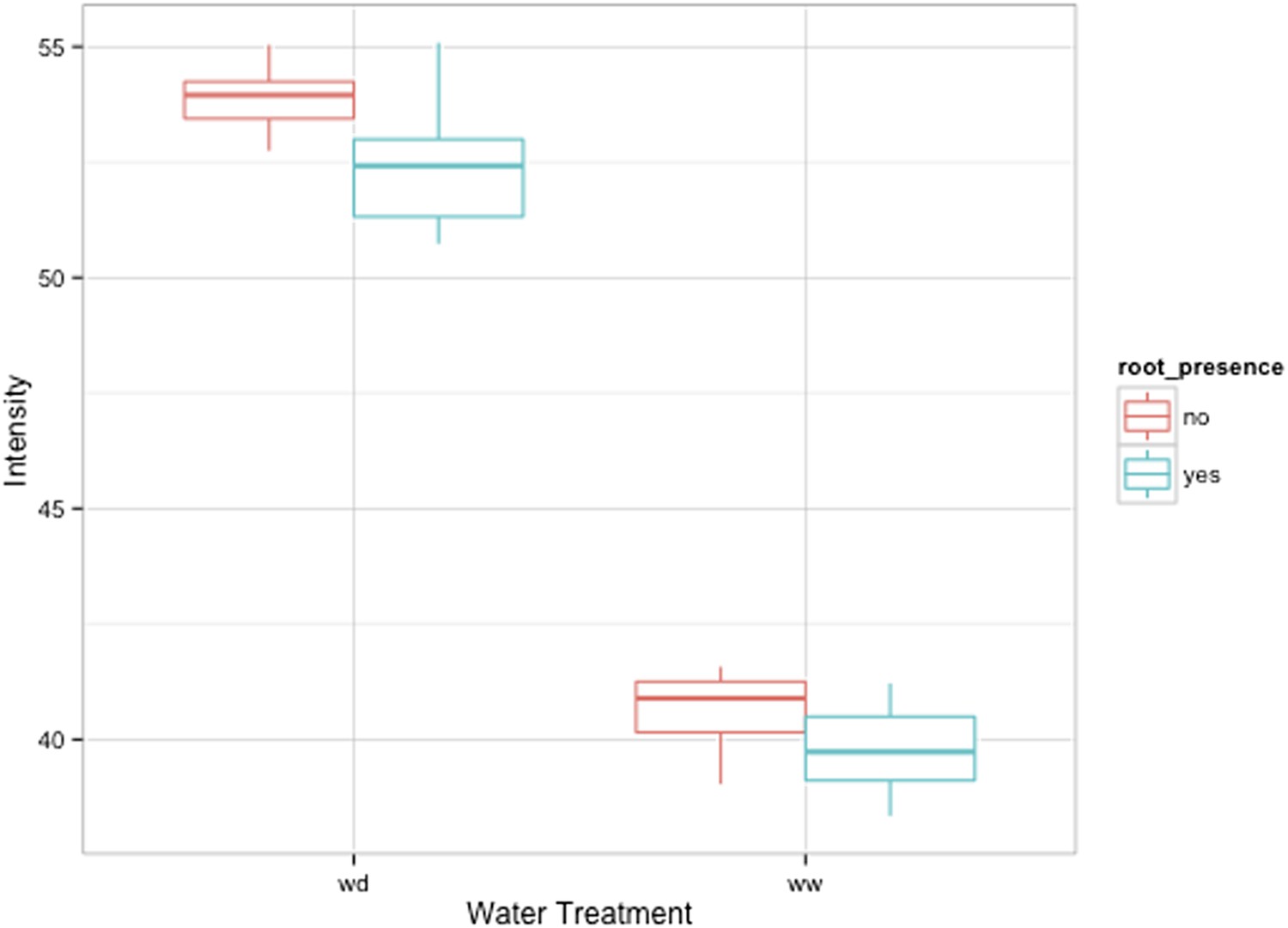
Comparison of soil intensity values between areas of the rhizotron with or without the presence of roots, determined based on luminescence data.
Mean intensity values from 100 × 100 pixel squares samples of both areas were obtained from 10 different rhizotrons. Wilcoxon test analysis with p < 0.01 showed no significant differences between areas with our without root presence.
Figure 6 with 5 supplements
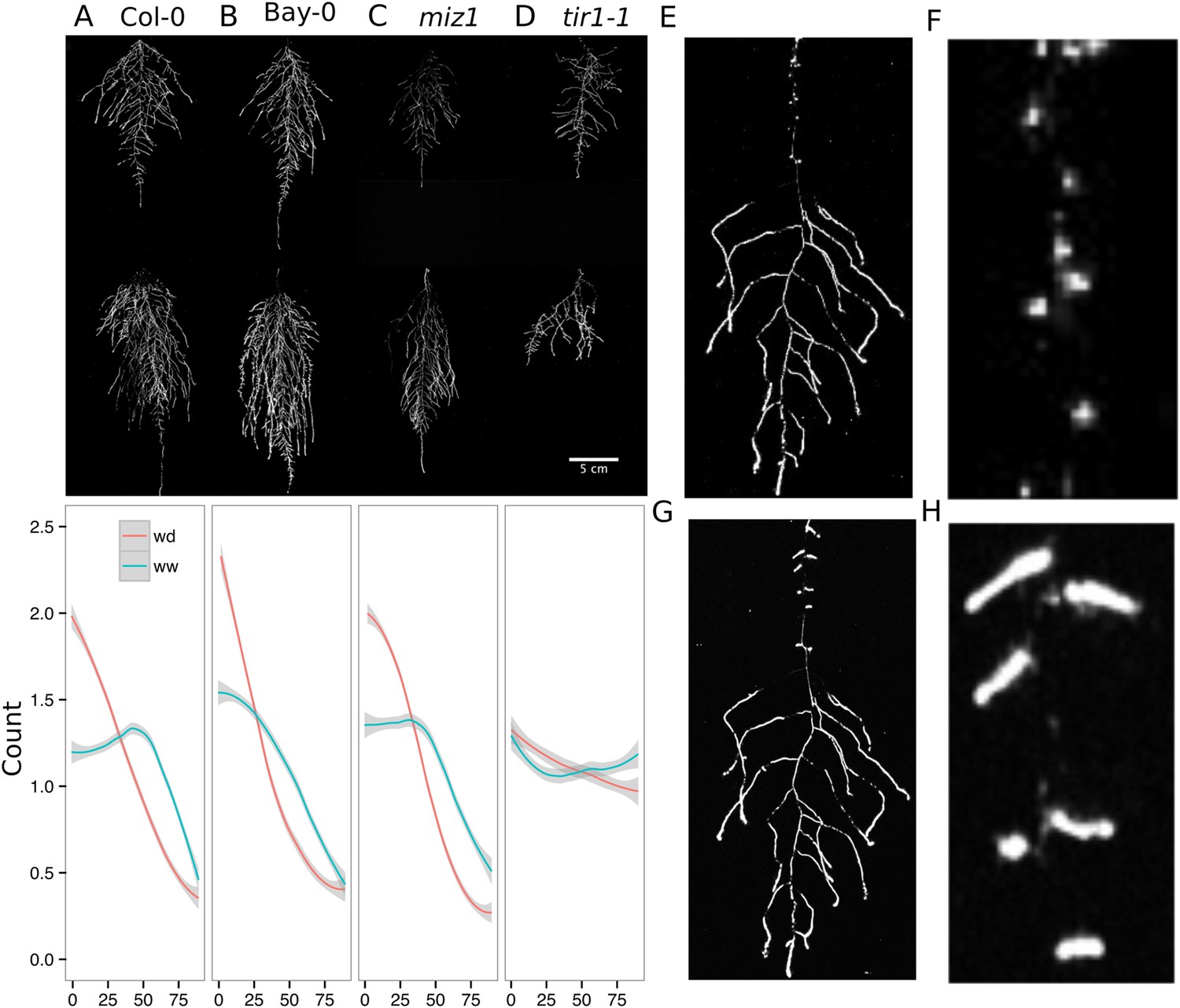
Study of effect of water deficit on root system architecture.
(A–D) Root systems 22 DAS and exposed to water deficit 13 DAS onwards (n = 8-9 plants). Sample images of WW (upper panels) and WD (lower panels) root systems treated from 13 DAS and directionality (line graphs to left of images) for (A) Col-0 (B) Bay-0 (C) miz1 and (D) tir1-1. (E) Root system of a 22 DAS plant exposed to water deficit from 9 DAS onwards with magnified view of lateral root primordia (F). (G) The same root as in (E) 24 hr after re-watering and magnified view of lateral roots (H). Kolmogorov–Smirnov test at p < 0.001 showed significant differences in directionality distributions between the WW and WD conditions for all genotypes except miz1. A local polynomial regression fitting with 95% confidence interval (gray) was used to represent the directionality distribution curve. 0° is the direction of the gravity vector.
-
Figure 6—source data 1
Directionality values of Bay-0, Col-0, miz1, tir1-1 grown under WW, WD and high and control temperature conditions.
- https://doi.org/10.7554/eLife.07597.038
-
Figure 6—source data 2
Directionality, root system architecture traits and shoot area values of Col-0 plants grown under different phosphorus concentrations.
- https://doi.org/10.7554/eLife.07597.039
-
Figure 6—source data 3
Directionality values of Col-0 and phot1/2 plants grown with the root system in the dark or exposed to light in the top third of the rhizotron.
- https://doi.org/10.7554/eLife.07597.040
-
Figure 6—source data 4
Directionality values at different depths of the rhizotron for Col-0 plants exposed to light in the top third of the rhizotron.
- https://doi.org/10.7554/eLife.07597.041
-
Figure 6—source data 5
Relative water content of leaves from plants grown under WW and WD conditions and high or control temperatures.
- https://doi.org/10.7554/eLife.07597.042
Figure 6—figure supplement 1
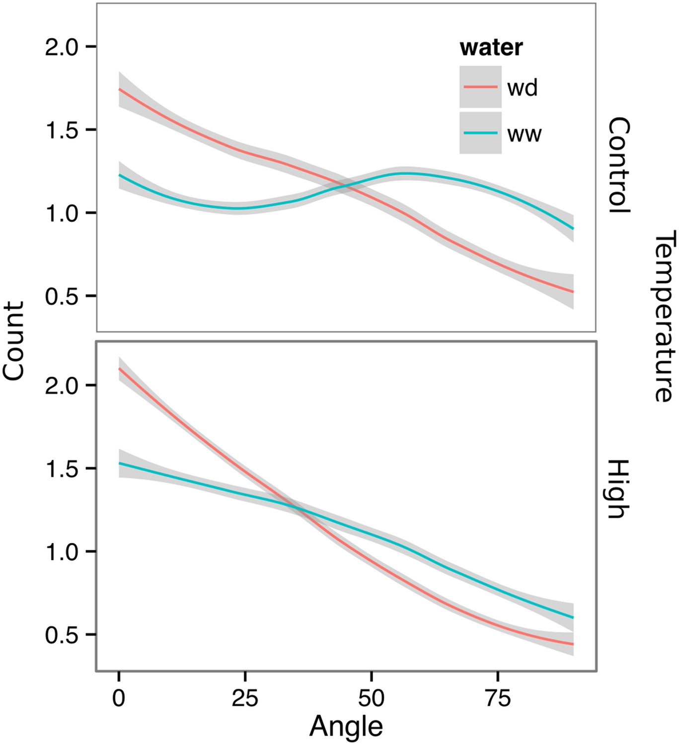
Directionality analysis of roots of plants transferred to WD conditions after 9 DAS and kept 22°C (control temperature) or 29°C (high temperature) until 22 DAS.
0° is the direction of the gravity vector. Kolmogorov-Smirnov test showed significant differences (p < 0.001) in the directionality distributions between WW and WD for both control and high temperature treatments. A Local Polynomial Regression Fitting with 95% confidence interval (grey) was used to represent the directionality distribution curve.
Figure 6—figure supplement 2
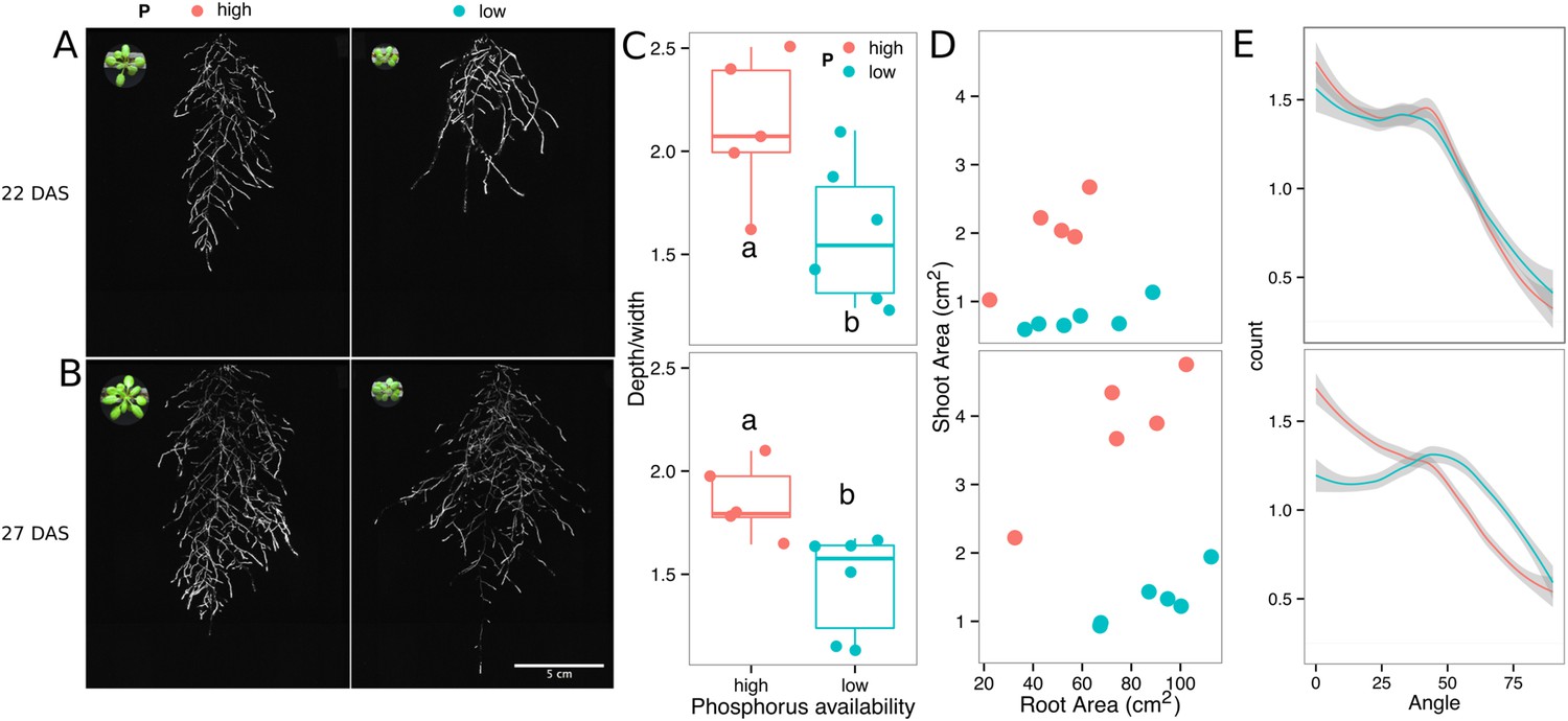
Phosphorus deficiency response of root systems.
Shoot and root systems of ProUBQ10:LUC2o Col-0 plants growing in soil supplemented with 1 ml of 100 μM P-Alumina (left) and 0-P-Alumina (right) 22 (A) or 27 (B) DAS (n = 5-6 plants). (C) Root depth/width ratio of 22 (top) and 27 (bottom) DAS plants. (D) Scatter-plot showing relationship between root and shoot system area at 22 (top) and 27 (bottom) DAS. (E) Root directionality distribution in plants 22 (top) and 27 (bottom) DAS. ANOVA analysis at p < 0.01 was used to compare depth/width ratios in P treatments. Kolmogorov–Smirnov test at p < 0.001 was used to compare directionality distributions between the different treatments. Distributions were significantly different at 27 DAS but not at 22 DAS. A local polynomial regression fitting with 95% confidence interval (gray) was used to represent the directionality distribution curve. 0° is the direction of the gravity vector.
Figure 6—figure supplement 3
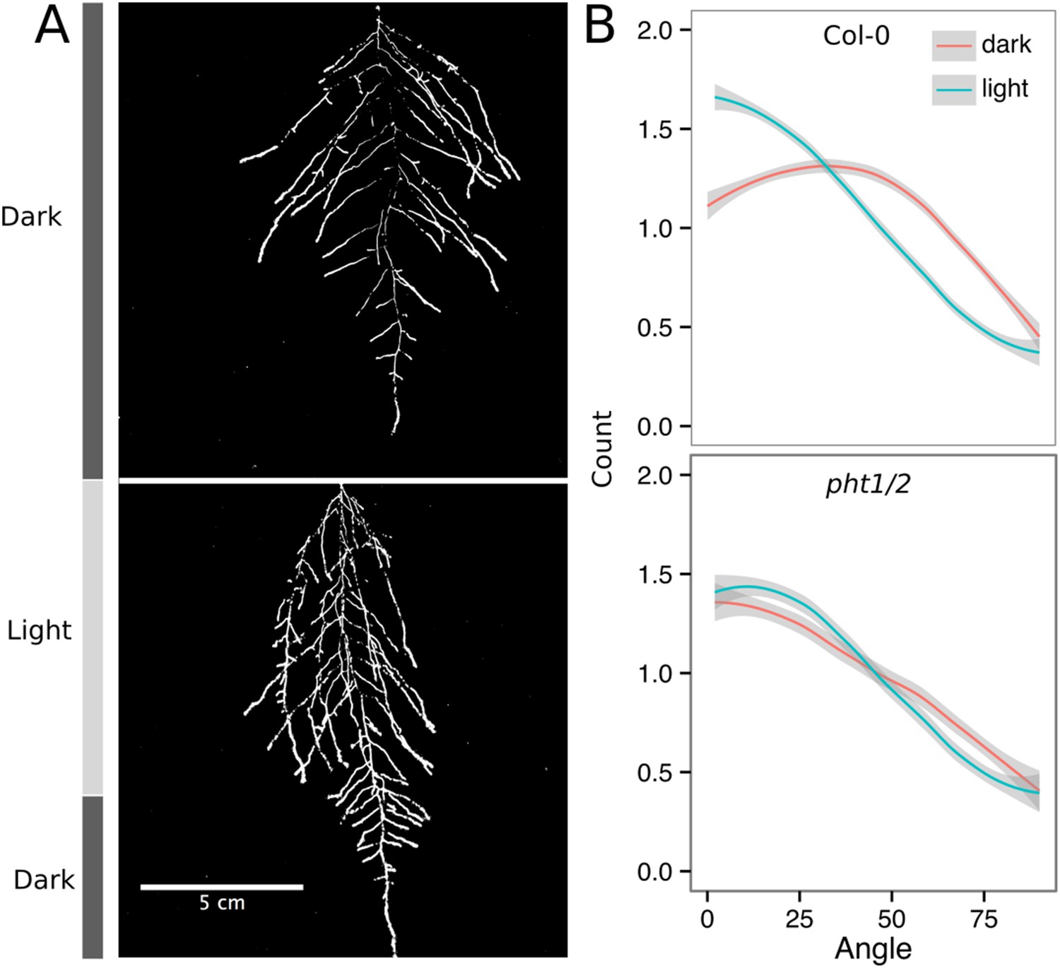
Effect of light on root directionality.
(A) Col-0 root systems shielded (top) or light exposed (bottom). After 9 DAS, the top third of the rhizotron was exposed to light (indicated on the side with a light gray bar) and plants were imaged at 20 DAS. (B) Directionality analysis of root systems shielded (red) or exposed (green) to light for Col-0 (top panel) or phot1/2 double mutant (bottom panel) (n = 4-6 plants). Between four and six plants were analyzed per treatment. ANOVA analysis at p < 0.01 was used to compare depth/width ratios in P treatments. Kolmogorov–Smirnov test at p < 0.001 showed significant differences in the directionality distributions between dark and light exposed Col-0 plants but not photo/2. A local polynomial regression fitting with 95% confidence interval (gray) was used to represent the directionality distribution curve. (0° is the direction of the gravity vector.)
Figure 6—figure supplement 4
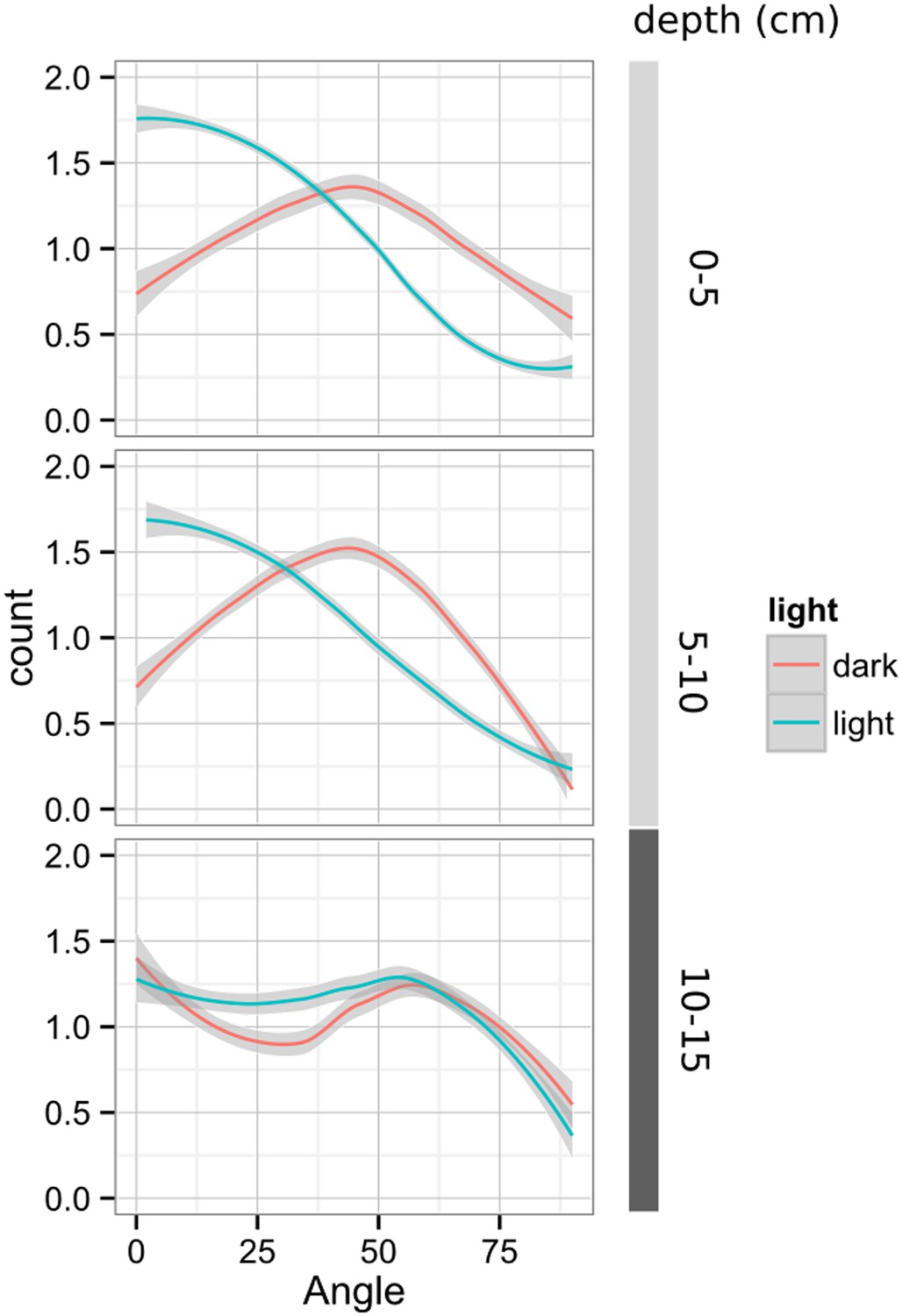
Plots showing output of directionality analysis performed at different depths (0–5, 5–10, 10–15 cm) in rhizotrons exposed to light or kept in the dark (n = 4-6 plants).
Kolmogorov-Smirnov test at p < 0.001 showed significant differences in the directionality distributions between dark and light exposed Col-0 plants at 0-5 and 5-10 cm of depth, but not at 10-15 cm. A Local Polynomial Regression Fitting with 95% confidence interval (grey) was used to represent the directionality distribution curve. 0° is the direction of the gravity vector.
Figure 6—figure supplement 5
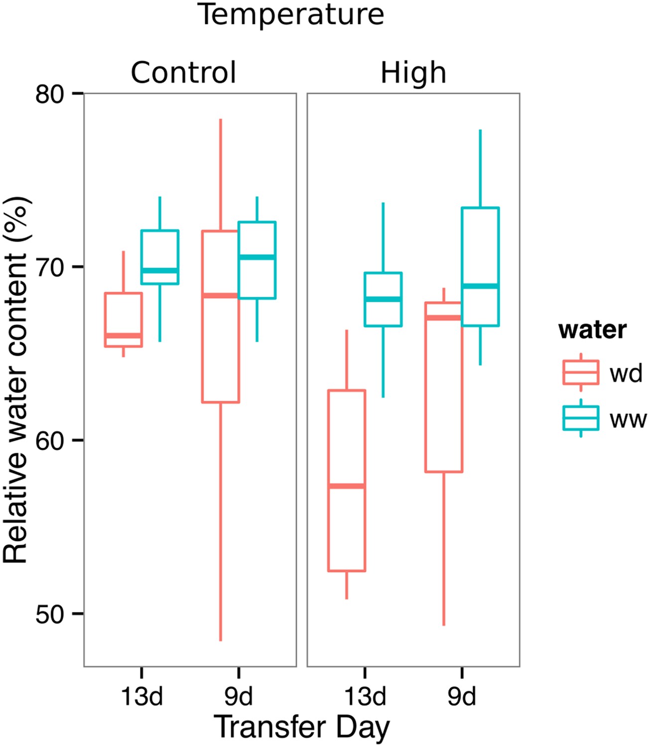
Leaf relative water content of 23 DAS plants that were subjected to WD after 9 or 13 DAS or kept under WW conditions.
At 9 DAS, half of the plants were kept under control temperature conditions (22°C) and the other half transferred to a 29°C (high) chamber (n = 6–8 plants). ANOVA at p < 0.01 showed no significant differences between WW and WD in either of the temperature conditions.
Figure 7
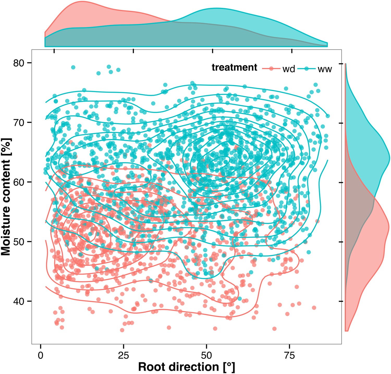
Relationship between local soil moisture content and root growth direction.
Data quantified from the time-lapse series are shown in Video 2. Density plots shown at periphery of graph for root direction (x-axis) and soil moisture (y-axis). 0° is the direction of the gravity vector. Data represent 2535 root tips measured in a series encompassing 10 time points.
-
Figure 7—source data 1
Individual root segment traits of plants growing under WW and WD conditions.
- https://doi.org/10.7554/eLife.07597.050
Figure 8 with 1 supplement
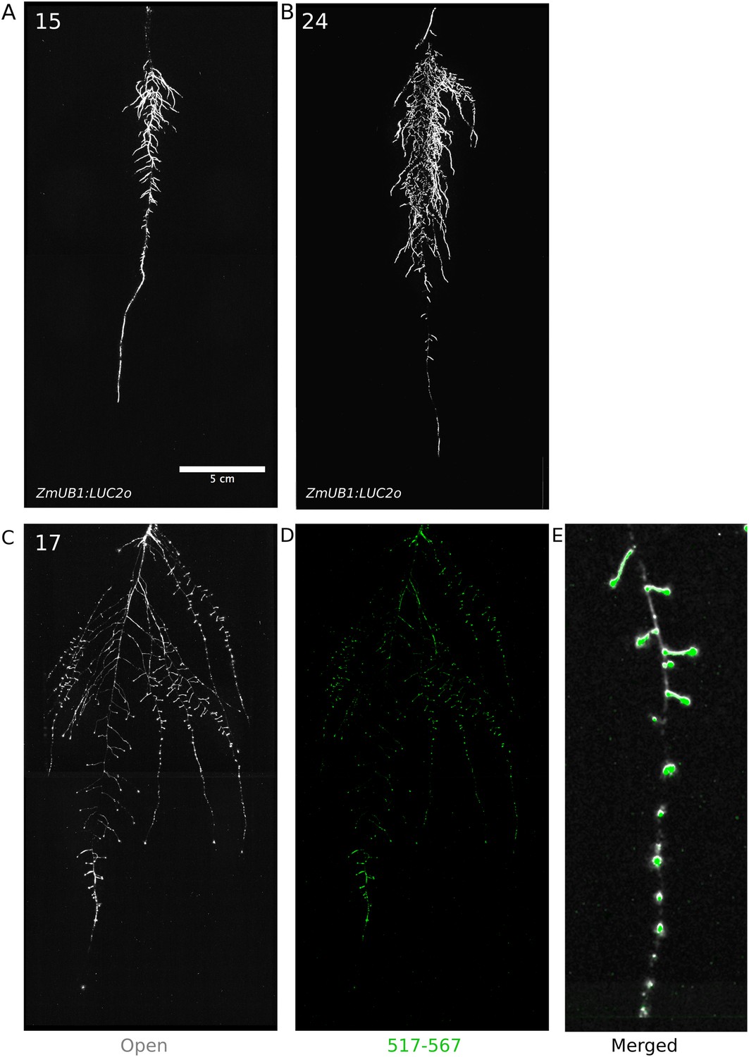
Roots of Brachypodium distachyon transformed with ProZmUB1:LUC2o and imaged at 15 (A) and 24 (B) DAS grown in control conditions.
(C) Open channel of 17 DAS tomato plant transformed with ProeDR5rev:LUC2o and Pro35S:PPyRE8o. (D) Green channel showing only ProeDR5rev:LUC2o. (E) Amplification of the open and green channel showing increased expression of ProeDR5rev:LUC2o reporter in early-stage lateral roots.
-
Figure 8—source data 1
Depth of Brachypodium primary roots grown in petri plates and rhizotrons.
- https://doi.org/10.7554/eLife.07597.052
Figure 8—figure supplement 1

Depth of the primary root of Brachypodium plants grown in rhizotrons or on gel-based media (n = 8–11).
Red dots indicate mean values.
Author response image 1

Videos
Video 1
Time lapse from 11 to 21 DAS of a Col-0 plant expressing ProUBQ10:LUC2o grown in control conditions.
https://doi.org/10.7554/eLife.07597.019
Video 2
Time lapse from 16 to 24 DAS of Col-0 plants expressing ProUBQ10:LUC2o growing in water-deficient (left) and control (right) conditions.
Plants were sown under control conditions and water-deficit treatment started 11 DAS. Images were taken every day.
Tables
Table 1
Luciferases used in this study
| Luciferase | Origin | Maximum wavelength | Substrate |
|---|---|---|---|
| PpyRE8 | Firefly | 618 | D-luciferin |
| CBGRed | Click beetle | 615 | D-luciferin |
| Venus-LUC2 | FP + firefly | 580 | D-luciferin |
| LUC(+) | Firefly | 578 | D-luciferin |
| CBG99 | Click beetle | 537 | D-luciferin |
| Lux operon | A. fischeri | 490 | Biosynthesis pathway encoded within operon |
| NanoLUC | Deep sea shrimp | 470 | Furimazine |
Table 2
List of root system features extracted using GLO-RIA
| Variable | Unit |
|---|---|
| Projected area | cm2 |
| Number of visible roots | – |
| Depth | cm |
| Width | cm |
| Convex hull area | cm2 |
| Width | cm |
| Feret | cm |
| Feret angle | ° |
| Circularity | – |
| Roundness | – |
| Solidity | – |
| Center of mass | cm |
| Directionality | ° |
| Euclidean Fourier descriptors | – |
| Pseudo landmarks | – |
Additional files
-
Supplementary file 1
Blueprints of the holders, clear sheets, and spacers needed to build the rhizotrons. Additional details are provided in the ‘Materials and methods’. Files are provided in Adobe Illustrator .ai and Autocad .dxf formats.
- https://doi.org/10.7554/eLife.07597.054
-
Supplementary file 2
Primers used in the qPCR experiment.
- https://doi.org/10.7554/eLife.07597.055
-
Supplementary file 3
Vector maps of all the constructs used in this work.
- https://doi.org/10.7554/eLife.07597.056
Download links
A two-part list of links to download the article, or parts of the article, in various formats.
Downloads (link to download the article as PDF)
Open citations (links to open the citations from this article in various online reference manager services)
Cite this article (links to download the citations from this article in formats compatible with various reference manager tools)
GLO-Roots: an imaging platform enabling multidimensional characterization of soil-grown root systems
eLife 4:e07597.
https://doi.org/10.7554/eLife.07597


