the Creative Commons Attribution 4.0 License.
the Creative Commons Attribution 4.0 License.
 | 07 Mar 2024
Modelling long-term industry energy demand and CO2 emissions in the system context using REMIND (version 3.1.0)
Felix Schreyer
Gunnar Luderer
This paper presents an extension of industry modelling within the REMIND integrated assessment model to industry subsectors and a projection of future industry subsector activity and energy demand for different baseline scenarios for use with the REMIND model. The industry sector is the largest greenhouse-gas-emitting energy demand sector and is considered a mitigation bottleneck. At the same time, industry subsectors are heterogeneous and face distinct emission mitigation challenges. By extending the multi-region, general equilibrium integrated assessment model REMIND to an explicit representation of four industry subsectors (cement, chemicals, steel, and other industry production), along with subsector-specific carbon capture and sequestration (CCS), we are able to investigate industry emission mitigation strategies in the context of the entire energy–economy–climate system, covering mitigation options ranging from reduced demand for industrial goods, fuel switching, and electrification to endogenous energy efficiency increases and carbon capture. We also present the derivation of both activity and final energy demand trajectories for the industry subsectors for use with the REMIND model in baseline scenarios, based on short-term continuation of historic trends and long-term global convergence. The system allows for selective variation of specific subsector activity and final energy demand across scenarios and regions to create consistent scenarios for a wide range of socioeconomic drivers and scenario story lines, like the Shared Socioeconomic Pathways (SSPs).
- Article
(5081 KB) - Full-text XML
- BibTeX
- EndNote


The targets of the Paris Accord (United Nations, 2015) (keeping global warming well below 2 °C while pursuing efforts to limit it to below 1.5 °C) have been shown to entail limited budgets of future CO2 emissions (Meinshausen et al., 2009; Pathak et al., 2022; Matthews and Caldeira, 2008). The CO2 budget for reaching the 1.5 °C limit with a likelihood of 50 % was estimated to be around 500 Gt CO2 by the latest IPCC assessment report (Arias et al., 2021). Similarly, limiting warming to below 2 °C with a 67 % likelihood – a possible interpretation of the well below 2 °C target (United Nations Environment Programme, 2022) – is assessed to constrain future cumulative CO2 emissions to 1150 Gt CO2. While these estimates are highly uncertain in size (Rogelj et al., 2019), it is evident that they are so constrained as to be unattainable without carbon dioxide removal (CDR) (Luderer et al., 2018). The availability of CDR, however, is uncertain (Fuss et al., 2018; Minx et al., 2018; Smith et al., 2015) and subject to major sustainability concerns (Smith et al., 2015). Therefore, minimising residual fossil CO2 emissions from the energy supply, building, industry, and transport sectors is imperative to limit reliance on CDR.
In 2020, industry accounted for 26 % of global CO2 emissions from fuel combustion and processes (International Energy Agency, 2021) and is the largest-emitting demand sector. Industry is broadly considered a decarbonisation bottleneck. Low-carbon solutions exist for almost all industrial processes, but decarbonisation is stymied by high abatement costs, inertia caused by the longevity of installations and technology development, and limited availability of (low-cost) low-carbon energy inputs (Deason et al., 2018; Bashmakov et al., 2022). While technological options for electrifying most industrial uses of fuels are available or are in the foreseeable future (Madeddu et al., 2020), their implementation depends on reductions in high electricity prices (relative to fossil fuels) (Luderer et al., 2022). Widespread electrification of industry, together with rapid decarbonisation of power supply, would alleviate most of the combustion emissions of the sector, leaving process emissions (e.g. reduction of iron ore, calcination of limestone), which need to be addressed by either negative emissions or modified process designs. A major driver of industry activity and emissions is the demand for industrial goods and services, which underpins both economic growth and increasing consumption levels, and demand reductions are discussed as a climate mitigation option (Bashmakov et al., 2022).
In view of the importance of the industry sector in terms of energy demand and CO2 emissions, its accurate modelling in the context of the overall energy transition is crucial for deriving meaningful climate change mitigation pathways in line with the Paris climate targets. Also, the industry sector competes with other sectors – buildings, transportation, and energy supply – for low-carbon energy, a dwindling carbon budget, and finite geological capacity for carbon sequestration. The transformation of industry therefore needs to be analysed in the context of these other systems (energy production, other energy demand sectors, and CO2 management options). Integrated assessment models (IAMs) provide a combined perspective on the integrated energy–economy–climate system.
So far, IAMs have pursued either a top-down approach with strong limitations in the granularity of the industry subsector and process representation or a stronger bottom-up representation of processes at the expense of a complete representation of system integration, e.g. in terms of macroeconomic substitutions, implications for material demand, and the impact of climate policies on economic growth.
We here present a newly developed industry sector module for the REMIND model which seeks to represent characteristics of processes in key subsectors while at the same time fully embedding the industry sector in the modelling of the transformation of the energy–economic system. Specifically, the new module explicitly represents the cement, chemical, steel production (split into primary and secondary production), and other combined industry subsectors. It models CCS individually per subsector, switching to advanced final energy carriers (hydrogen and electrification of high-temperature heat provision) and energy efficiency investments, and links the industry sector to macroeconomic demand drivers as well as final energy provision and carbon management of a detailed bottom-up energy system model. The new module thus covers all major mitigation options for industry, ranging from end-of-pipe approaches to fuel switching, electrification, efficiency, and macroeconomic adjustments in response to climate policy.
There is a lack of integrated assessment models representing price and economic feedbacks on industrial demand as well as efficiency, fuel switching, and CCS options in industrial activities. In this respect, the extended industry sector in the REMIND model compares favourably to other IAMs. A forthcoming overview of industry CO2 emission reduction (Bauer et al., 2024) compares seven IAMs “with improved industry sector representation”. They all represent at least the cement, chemical, and steel production subsectors and to varying degrees mitigation options like energy efficiency improvements, final energy substitution, and CCS. The endogenous reduction in industry demand as a trade-off with other mitigation options is a feature of general equilibrium models (two out of the seven models: GEM-E3 (Fragkos and Fragkiadakis, 2022) and REMIND). Partial equilibrium models (COFFEE (Rochedo, 2016), MESSAGEix (Grubler et al., 2018), IMAGE (van Sluisveld et al., 2021), POLES (Després et al., 2018), and PROMETHEUS (Fragkos et al., 2015)) rely on exogenous demand pathways for policy scenarios and are typically inelastic to changes in CO2 and thus energy prices. The WITCH model (The WITCH team, 2017) is an example of another general equilibrium IAM but only represents an aggregated stationary sector and not a separate industry sector.
Further to the refinements of industry sector representation within REMIND, we present new methods for producing consistent trajectories for industry subsector production and final energy use for different baseline scenarios used for calibrating the REMIND model. They project per-capita subsector activity based on per-capita gross domestic product (GDP) projections and allow for variation in material and energy intensity to derive different scenarios.
2.1 REMIND model structure
The integrated assessment model REMIND (Baumstark et al., 2021) is comprised of a macroeconomic growth model and a detailed energy system model (ESM) which are hard-linked, i.e. optimised simultaneously, with energy supply (by the ESM) and demand (by the macroeconomic model) quantities and prices in equilibrium. The ESM represents over 50 conventional and low-carbon energy conversion technologies, modelling energy flow from primary through secondary to final energy, accounting for CO2 and other greenhouse gas (GHG) emissions as well as carbon capture and sequestration (CCS), carbon capture and utilisation (CCU), and options for carbon dioxide removal (CDR). The macroeconomy is represented by an intertemporal general equilibrium model that maximises the intertemporal welfare of 12 to 21 world regions (depending on parametrisation) that are linked by trade of primary energy carriers, an aggregated trade good, and emission permits. The macroeconomic model uses a nested constant elasticity of substitution (CES) production function (Chung, 1994), in which labour, energy, and capital are used for the production of economic output, and energy inputs are tracked through the building, industry, and transport economic sectors to final energy carriers which constitute the links to the ESM. The different economic sectors form sub-trees in the CES function and can be realised in different levels of detail. This paper describes specifically the extension of the industry sector from an aggregated realisation to one in which different subsectors are modelled explicitly. The nested CES production function takes the following form:
where Vo1 is the output quantity, Vi are the input quantities, αi are efficiency parameters for the inputs, and ρo is a parameter derived from the substitution elasticity σo () between the inputs on a CES nest. The set CES of tuples (o,i) links the output of a CES nest to its inputs. Since outputs on one level are inputs on another, this gives rise to a tree structure (see Fig. 1). Substitution elasticity σ in general describes the relative change in utilisation of the inputs to an economic production process (called production factors) in relation to the relative change in input prices. A function with constant elasticity of substitution assumes that a specific percentage increase (decrease) in the price of one production factor in relation to the prices of the other factors will cause a constant specific percentage decrease (increase) in factor utilisation, irrespective of the amount of factor utilisation at which this price change occurs.
Operating the REMIND model entails calculating a baseline scenario, in which no climate change mitigation policies are assumed, and then imposing different constraints on the model (e.g. a fixed carbon price trajectory, a limit on peak or end-of-century temperature increase, or a limited greenhouse gas emissions budget over the century) for calculating policy scenarios that are used to investigate specific research questions (e.g. the feasibility of climate change mitigation targets under constrained availability of technologies, the impact of climate change mitigation policy on investments in certain technologies, and the macroeconomic costs of different climate change mitigation regimes) (Baumstark et al., 2021). Besides initialising a large set of variables (i.e. all stocks of energy conversion technologies in the ESM, their efficiency parameters, and trade in all traded goods) for the first model time step (2005), this requires determining the efficiency parameters αi for the CES production function for the entire model time horizon. For this, trajectories for the output (macroeconomic production – GDP) of the CES production function and all inputs (final energy demand and for industry also subsector production levels) into the CES production function over the entire model time horizon (until 2100) are needed.
In addition to extending the industry sector in the REMIND model itself, it is also necessary to calculate consistent trajectories for the input data of the CES calibration (subsector production and final energy demand) for different baseline scenarios of future development (see Sect. 3.1).
2.2 Industry subsectors
The CES production function of REMIND can be expanded to explicitly represent the industrial subsectors and economic drivers for the demand of their products. The industry sector of the REMIND model is split into four subsectors: cement2, chemicals, steel production, and all “other industry” production, based on the energy demand characteristics of the sectors, their portion in industry energy demand and CO2 emissions, and the applicability of CCS.
The products of both the cement and the steel subsectors are comparatively homogeneous with well-defined properties, for which country-level statistics in physical units are available, and the subsectors are dominated by a few production processes. The chemical subsector produces a diverse range of intermediate and final products, yet some energy-intensive processes (e.g. steam cracking or reforming) are common to many production routes (Fischedick et al., 2014). Since production statistics for the different products are not widely available and the products lack commensurability with respect to energy inputs and CO2 emissions of production, a monetary measure is employed to model the activity of the chemical subsector. The last subsector, other industries, is by definition characterised by diverse processes and heterogeneous goods which are not comparable on a physical basis, and therefore a monetary measure is used for modelling its activity, too. The decarbonisation challenges faced by the other industry subsector are, however, quite comparable, as most of the energy demand can be electrified by established technologies (Madeddu et al., 2020).
Using value added instead of physical production to drive industry energy demand incurs two difficulties. Both the specific value added per unit of (physical) production and the composition of different types of products making up subsector production vary across regions and change over time. This reduces the interpretability of subsector production figures given in value-added production, especially in absolute terms. However, it does not impinge on the usefulness of linking economic activity and industry energy demand, as the historical regional differences are subsumed by the regression of subsector energy demand on subsector activity, and the composition of subsector production is expected to move in the direction of higher shares of high-value products (decreasing physical production per unit value added) as economies evolve to higher GDP per capita, which acts in the same way of increasing energy efficiency (decreasing energy demand per unit of physical production), not introducing behaviour that is different from subsectors with physical representation.
The production of cement, chemicals, and iron and steel consumes the bulk of final energy in the industry sector (7 %, 14 %, and 23 %, respectively (Fischedick et al., 2014)) and accounts for 29 %, 13 %, and 30 % of total direct CO2 emissions of industry (8.7 Gt CO2 yr−1) (International Energy Agency, 2021). The application of CCS in industry has been studied for different subsectors (Kuramochi et al., 2012), but due to the limited number of key processes, the large average size of installations (which are economic point sources), and the high specific CO2 emissions by unit of economic output, the cement, chemical, and steel subsectors are considered to be the main targets of CCS in industry (Naims, 2016).
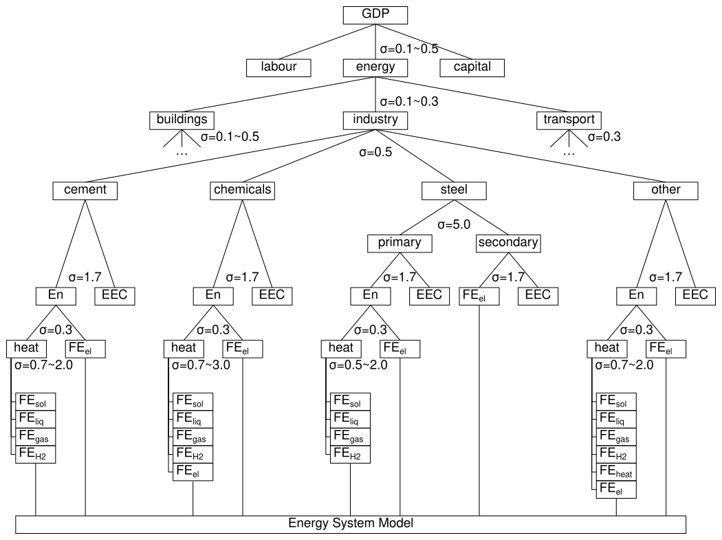
Figure 1REMIND CES production tree. Macroeconomic output (GDP) is produced from labour, energy (energy services), and capital, while energy services are subdivided into the industry sector and the building and transport sectors (both omitted for clarity). The cement, chemical, steel, and other industry subsectors use final energy (FE) provided by the energy system model and energy efficiency capital (EEC) to provide energy services. σ denotes substitution elasticities between the respective inputs into a node, with denoting elasticities changing over time.
2.3 Electrification of heat production
Energy use in industry can roughly be subdivided into two categories: energy for mechanical work, provided principally by electricity, and energy for heating, provided principally by fuels – especially on medium to high temperature levels (above 100 °C). Both are represented in REMIND through individual nodes in the CES production structure of the industry subsectors, with low elasticities between them, as mechanical work and heat are not interchangeable in production processes. The substitution elasticities of fuels increase from low to high levels (0.5 or 0.7 to 2) by 2040, reflecting lower short-term and higher long-term flexibility in industry. Since the electrification of heat production is technically possible (Madeddu et al., 2020) and a viable option for mitigating CO2 emissions (when using carbon-free electricity), we include an additional production factor for high-temperature heat from electricity in the production functions for both the chemical and other industry subsectors (see Fig. 1).
This allows for the explicit modelling of the substitution between fuels and electricity in heat production, without allowing for the replacing of mechanical work through heat. This option is only included for the chemical and other industry subsectors, since electric steel production is modelled explicitly (see Sect. 3.3), and electrification of clinker burning (a major source of CO2 emissions in cement production) is less attractive compared to CCS options because it would only mitigate emissions from fuel burning, while large process emissions from limestone calcination (about half of total emissions) would remain (or require additional CCS).
The representation of energy carrier switching via the CES production function takes into account the heterogeneity of circumstances in industry subsectors, with some better positioned to electrify high-temperature heating than others.
2.4 Energy efficiency investments
We also introduce dedicated stocks for energy efficiency capital (EEC) for all industry subsectors. They are positioned at the top level such that subsector output is produced from the aggregated energy inputs and the EEC (see Fig. 1). This models the trade-off between capital investment and energy demand. It is possible to invest in facilities with higher energy efficiency (usually for new installations, to some degree also for retrofits). This capital stock is integrated into the handling of the macroeconomic capital stock in REMIND and is subject to depreciation and requires investments (Baumstark et al., 2021).
Both the stock of and the investments in capital for energy efficiency, separate from the general capital for industrial production, are difficult to ascertain (International Energy Agency, 2014). We therefore initialise this stock from investment estimates into energy-intensive (cement, chemicals, steel) and non-energy-intensive industry (other industry) for 2014–2020 (International Energy Agency, 2014, Annex A), assuming a steady state where energy efficiency investments only cover the depreciation of the EEC stock, which is assumed to depreciate exponentially with a half-life of 25 years. For the baseline scenarios, we assume EEC will grow (and shrink) proportional to subsector output (but EEC stocks are not reduced beyond the depreciation rate – in accordance with the capital motion formulation of the REMIND model).
2.5 Representation of mitigation options
Expanding on Kaya et al. (1997) and Fischedick et al. (2014), industry decarbonisation can be analysed using the following identity:
where E values are the emissions, Pop the population, GDP the economic activity, A the industrial production, FE the final energy use in industry, FF the fossil fuels used in industry, and C the carbon content of those fossil fuels. The products of the identity are drivers of emissions or mitigation options: Pop – population growth (or more generally population change); – per-capita GDP (affluence); – the share of industry in economic activity (as opposed to agriculture and services); – the energy intensity of industry; – the share of fossil fuels in industry energy demand (as opposed to renewable energies); – the specific carbon content of those fuels per unit energy (high for coal and oil, lower for natural gas); and – the emissions rate, which can be reduced by CCS.
Different drivers and mitigation options are realised by different parts of the extended REMIND model as presented here. Population is an exogenous SSP scenario assumption and is thus constant across scenarios (that are based on the same SSP). GDP and industrial activity are endogenous elements of the production function and vary with the strictness of mitigation constraints. Final energy, fossil fuels, carbon content, and emissions are all endogenous elements of the ESM. Notably, the REMIND model covers the entire range of mitigation options, from reduced demand for industrial goods, increased energy efficiency in industry, fuel switching, and renewable power production to CCS.
A forthcoming overview of industry CO2 emission reduction (Bauer et al., 2024) compares seven integrated assessment models “with improved industry sector representation”, in which the REMIND model as discussed here shows the widest range of endogenous mitigation options. Notably, it is the only IAM with endogenous reduction in industry demand due to its integration of a Ramsey growth model.
2.6 Implementation of mitigation options in REMIND
The role of the industry module is to provide a hard link between a macroeconomic growth module and ESM, taking into account the aspects unique to industry (as opposed to the building and transport sectors). This entails (1) balancing industry final energy demand as an input to the CES production function with final energy provision by the ESM, (2) deriving industry outputs and activity levels consistent with the overall macroeconomic developments and climate policy constraints, (3) deriving final energy demand consistent with industrial outputs and activity levels, and (4) accounting for CO2 emissions and options for their abatement via CCS and consistency of industrial production with climate policy targets.
The first function is achieved by a simple balance equation that equates the sums of final energy inputs of different types (e.g. solids, liquids, and gases) into the different industry subsectors in the CES production function (Vi in Eq. 1) with the production of the final energy carriers in the ESM. In this way, production of industry output that consumes energy incurs costs for energy production in the ESM, which have to be covered from the macroeconomic production (i.e. GDP output of the production function).
CES production functions, being an economic concept, do not represent all physical aspects relevant to modelling physical production in industry. They allow for the substitution of production factors beyond limits that might exist in real technical applications. Specifically, the formulation involves industry subsector output being produced from energy and EEC, capturing the mechanism where investments in energy efficiency can reduce the specific energy demand per unit output, but only up to a limit, given technical and physical (thermodynamic) constraints. We therefore impose a lower bound of the sum of final energy inputs into a subsectors' CES sub-tree per unit of subsector output to confine the model solution space to technically and physically feasible values. This bound is described by an exponentially decreasing function that decreases from the 2015 specific energy demand towards the limit described below in Sect. 3.6 and passes through a point that allows climate change mitigation scenarios to close no more than 75 % of the gap between the baseline scenario and this limit in 2050.
CES production functions also do not deviate far from equilibrium points. This is a problem in the detailed representation of final energy carriers with CES functions, as the carriers not already in use will see little utilisation even at very high price levels. This is most relevant for hydrogen and electricity for high-temperature heat production in industry, both of which are economically unattractive without strict climate policies and accompanying high carbon prices, and have therefore not been used so far. To overcome this limitation, we employ two mechanisms.
First, we set future shares of hydrogen and high-temperature heat electricity for the baseline calibration. The share of hydrogen in industry gases is increased from 0.1 % in 2020 to 30 % in 2050. The share of high-temperature heat electricity in industry FE demand for high-temperature heat (so excluding electricity for mechanical work and low-temperature heat) is increased from 0.1 % in 2020 to 8 % in 2050. This leads to demand for hydrogen and high-temperature heat electricity in industry that is not in line with a “no climate change mitigation policy” baseline scenario but necessary to generate realistic policy scenarios.
Second, we apply mark-up costs to both hydrogen and high-temperature heat electricity use in industry to represent the additional cost of introducing new technologies into the production process that use these energy carriers.
Due to the economic nature of input substitution in the production function, the mark-up costs cannot be determined by techno-economic data and are instead set based on model behaviour. Both mechanisms, future baseline hydrogen and high-temperature heat electricity shares and mark-up costs, have been parametrised utilising the concept of the marginal rate of substitution, which describes the amount of one input needed to substitute another input to provide the same economic value (the ratio of the partial derivatives of two inputs into the production function). Final energy shares and mark-up costs are chosen such that the marginal rates of substitution with respect to gases and liquids (given the strong competition posed by the final energy carriers hydrogen and high-temperature heat electricity) roughly approach technical substitution ratios in climate policy scenarios (one for hydrogen, two to three for high-temperature electricity). The mark-up costs can be reduced in scenarios which e.g. stipulate a strong policy push for these technologies (Schreyer et al., 2024), making hydrogen and/or high-temperature heat electricity cheaper relative to other final energy carriers and in turn increasing their utilisation in industry.
Finally, we impose a lower bound on the share of steel from primary production (see Sect. 3.3 below).
Industry CCS is calculated by applying subsector-specific marginal abatement cost (MAC) curves. The MAC curves are based on either Kuramochi et al. (2012), who performed a techno-economic assessment of CO2 capture technologies with capture rates of 28 %–76 %, equating to USD2005 62–133 per tonne CO2 (note that all monetary values and prices in REMIND are denoted in US dollars for the year 2005 and are converted accordingly) for different subsectors, or Fischedick et al. (2014) (Fig. 10.7–10.10), who implemented a more optimistic industry CCS scenario (with capture rates of 75 %, corresponding to 50 t−1 CO2, in USD2005 and up to 95 %, corresponding to 217 t−1 CO2, in USD2005 for all subsectors except other industry subsectors). Subsector emissions from fuel combustion are calculated from final energy demand and fuel-specific emission factors. Process emissions in the cement subsector are calculated by applying a specific emissions factor for clinker (0.53 t CO2 t−1 clinker) and regional clinker to cement ratios (0.58–0.82 t−1 clinker t−1 cement; Kermeli et al. (2016), Fig. 21), which are converged towards the lowest regional value by 2100. The model is then able to capture industry CO2 emissions up to the level indicated by the respective MAC curve at given CO2 prices. Since the MAC curves do not reproduce the inertia of capital stocks required for CCS (investments and retrofits would occur only gradually, not all at once), the increase in the capture rate is limited to 5 % per annum.
3.1 General approach
Since there is structural uncertainty in the future development of the fundamental drivers of the energy system – population and GDP growth – IAMs use the Shared Socioeconomic Pathways (SSPs) as a common framework (O'Neill et al., 2017). The five SSPs (named SSP1 through SSP5) provide both contextual descriptions of how the world might evolve in the coming century and quantitative trajectories for future population and GDP on the country level. They are varied along two orthogonal axes: socioeconomic challenges to climate change mitigation and socioeconomic challenges to adaptation to climate change. In this paper, we consider the SSP1, SSP2, and SSP5 scenarios, updates from earlier SSP realisations, with the REMIND model (Kriegler et al., 2017).
-
The SSP2 scenario is characterised by median challenges along both axes and is referred to as a “middle-of-the-road” scenario, where historic trends continue into the future, improving living conditions for most people without pronounced reductions in global inequality and making technological progress at a steady but constant rate.
-
The SSP1 scenario is characterised by challenges considered low along both the mitigation and the adaptation axes and is referred to as a “sustainability” scenario, where the demographic transition is accelerated, leading to lower population growth; high-income countries shift to “a broader emphasis on human well-being”, leading to slower economic growth; and investments and adjusted tax incentives bring about faster progress in resource efficiency.
-
The SSP5 scenario is characterised by challenges considered high to mitigation but challenges considered low to adaptation and is referred to as a “fossil-fuel-development” scenario, where the exploitation of abundant fossil fuels drives investment in health and education, but also consumption, and therefore very energy-intensive lifestyles globally.
We project industry subsector activity, as well as final energy demand, for the SSP2 (middle-of-the-road) scenario, which best fits the continuation of historic trends into the future. All other scenarios, including SSP1 and SSP5, are derived as variations of specific material and specific energy demand of the SSP2 scenario.
Industry subsector activity (except for steel production) for the SSP2 scenario is projected in per-capita terms as a function of per-capita GDP in the form of
where ApC is the per-capita activity level, GDPpC the per-capita GDP, α the asymptotic limit of ApC, and β a parameter of convergence speed. This formulation is used because it presupposes a decoupling of per-capita demand from increasing affluence levels, and its positive codomain makes it easily tractable. In previous research it has been found to be a good fit to historic data (van Ruijven et al., 2016). A decoupling between GDP and production of bulk industrial goods (cement and steel) or the value added of industry (chemical and other industry subsectors) is in line with historically observed patterns and is generally assumed to continue as future economic activity moves from physical production to service provision (Bashmakov et al., 2022). The parameters α and β are derived via regression on both regional and global levels. The regional asymptote α is linearly converged towards the global value until 2200 (i.e. in about 2100 it lies half way between the original regional and global levels). This results in a short-term continuation of current trends and a long-term convergence across regions. Using these converged parameters, per-capita and absolute activity are projected using per-capita GDP and population projections (Koch and Leimbach, 2023; KC and Lutz, 2017).
For cement, activity levels are derived in physical units (production quantity); for the chemical industry they are expressed in economic units (subsector value added) due to the heterogeneity in the chemicals produced. Since cement and steel production is modelled in physical units, an additional regression of value added per unit production is performed (see Sect. 3.5). This allows for calculating consistent estimates for the other industry subsector as the difference between total industry value added and the value added of the cement, chemical, and steel subsectors. These regressions use the same formula as is used for per-capita output (Eq. 3), presupposing an increasing specific value added (USD per unit of production) that converges toward some level, as industry moves to production of increasingly higher-value products (e.g. high-strength or corrosion-resistant steels rather than generic construction steels). As before, the regression is performed on both the regional and the global level, and the regional asymptotic limit α is linearly converged towards the global value until 2200 (i.e. in about 2100 it lies half way between the original regional and global levels). Population and GDP regression data are from the World Bank (2019), series NY.GDP.MKTP.PP.KD (GDP, PPP; constant 2017 international dollars) and SP.POP.TOTL (population, total), from 1970 through 2021. Table 1 collects all data sources used for all or for individual subsector regressions and projections.
United Nations Department of Economic and Social Affairs Population Division (2015)World Bank (2019)Arujo et al. (2021)KC and Lutz (2017)Koch and Leimbach (2023)James et al. (2012)van Ruijven et al. (2016)USGS (2020)Müller et al. (2013)Pauliuk et al. (2013b)United Nations Industrial Development Organization (2017)United Nations Industrial Development Organization (2017)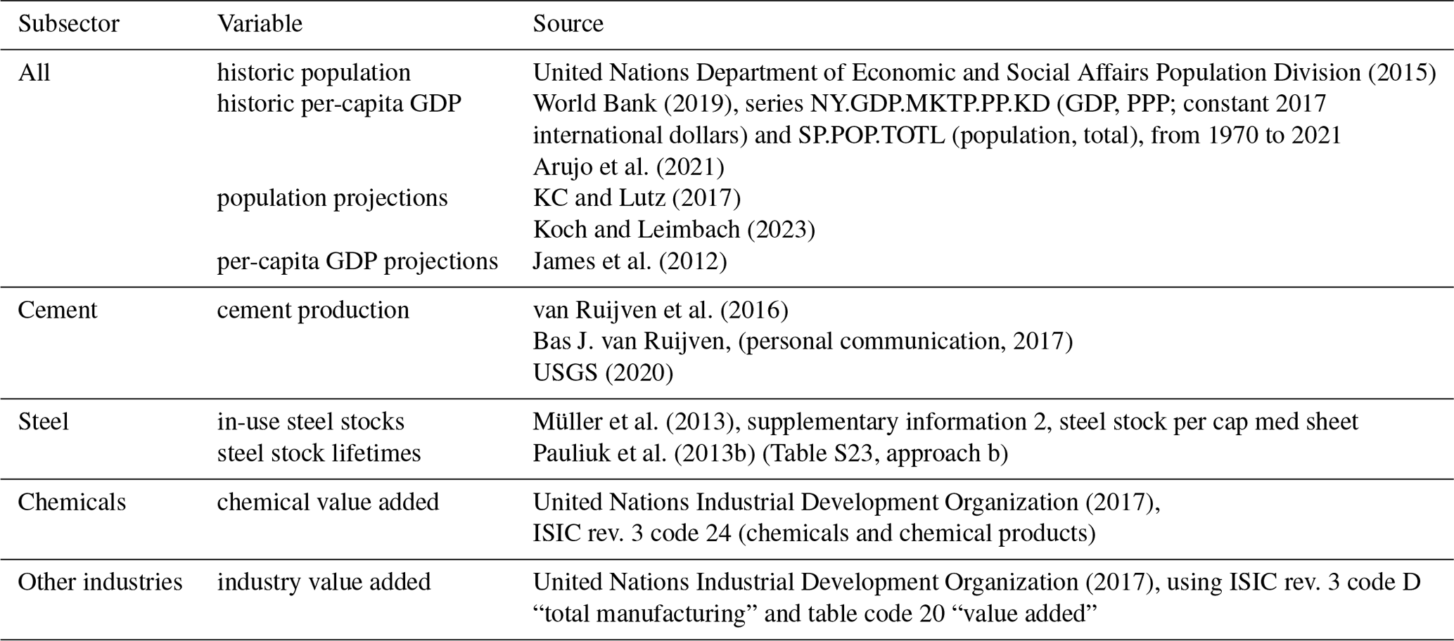
3.2 Cement projections
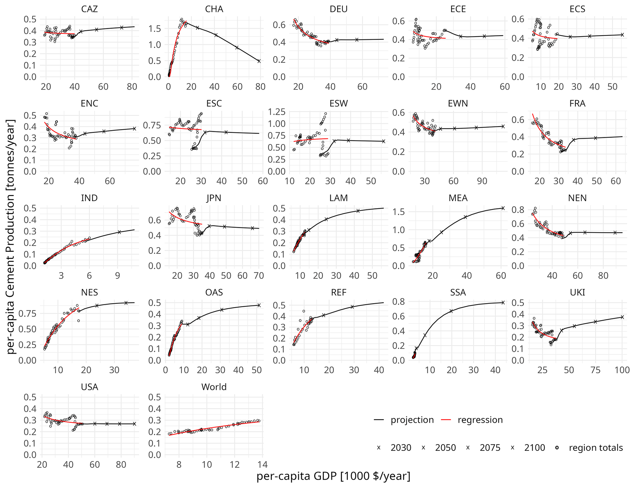
Historic per-capita cement production is regressed on per-capita GDP using the formulation discussed above (Eq. 3), using cement production summaries by van Ruijven et al. (2016), Bas J. van Ruijven, (personal communication, 2017), and USGS (2020). Regression parameters are derived once on the regional level and once again on the global level. For the global regression, cement production from the People's Republic of China with Hong Kong SAR and Macau SAR and the Republic of China (CHA) region is excluded, since the exceptional cement production of the People's Republic (55 % of global production at 18 % of the global population in 2019) would unduly bias the global regression. Projections of per-capita cement production and total cement production are calculated from the converged regression parameters (see above) and per-capita GDP as well as population projections for the SSP2 scenario, respectively. Figure 2 shows the regression data (regionally aggregated), the regression function, and the SSP2 projection.
3.3 Steel projections
Iron and steel differ from other bulk materials like cement and basic chemicals by being easily recyclable. Cement is bound in concrete with aggregate and possible reinforcement that requires elaborate separation and energy-intensive reversal of the hydration reactions during setting to be recycled. Chemicals like ethylene and propylene are processed into complex products like plastics that are widely dispersed in the economy, requiring careful separation from other materials and energy-intensive treatments to recover feedstocks or products that are often not of a comparable quality to the ones being recycled (Uekert et al., 2023). Steel can mostly be collected, separated magnetically from other materials, and molten down to produce new products. (There are important constraints on the quality of recycled steel due to tramp elements like copper (Daehn et al., 2017), currently limiting the share of recycled steel.) For these reasons, steel, unlike cement and chemicals, accumulates in the economy. Most iron ore that has been refined into steel stays available as steel.
Our projections of steel production therefore follow the approach of Pauliuk et al. (2013a), which considers the (per-capita) stock of steel in use in the economy and not the yearly flow of new steel being produced as primary regression variable. It assumes that in-use per-capita steel stocks will saturate over time and that deprecated stocks will then be replaced mainly by recycled steel. Projections of steel production derive from carrying forward the steel stocks; calculating yearly stock losses from deterioration to scrap; and, based on available scrap, calculating secondary and then primary steel production.
Estimates of in-use steel stocks per country (Müller et al., 2013, supplementary information 2, “steel stock per cap med” sheet) are aggregated to 21 regions and converted to per-capita numbers with population data (United Nations Department of Economic and Social Affairs Population Division, 2015) and then regressed on per-capita GDP (Arujo et al., 2021; World Bank, 2019) using the logistic function
where SpC is the per-capita steel stock, GDPpC the per-capita GDP, A the saturation level (asymptote) of per-capita steel stock, i the per-capita GDP level at which the steel stock is half as much as the asymptote (inflection point), and s a scaling parameter determining the speed of convergence. The resulting regression parameters A, i, and s are used with per-capita GDP projections from James et al. (2012) and population projections from KC and Lutz (2017) as well as Koch and Leimbach (2023) to project future per-capita and absolute steel stocks.
Projected steel stocks are depreciated exponentially with the steel stock lifetime l from Pauliuk et al. (2013b) (Table S23, approach b), which is converged linearly towards the global average in 2100. Of the depreciated steel stocks, we assume 90 % to be available for recycling. The resulting year-on-year differences in steel stocks (due to both per-capita steel stocks increasing monotonically with increasing per-capita GDP and replacements for depreciated stocks) are the required stock additions. Decreases in steel stocks due to shrinking populations are not balanced but ignored, as they would otherwise imply a reduced per-capita steel production in regions with contracting populations. (The lifetimes of steel stocks are largely independent of utilisation and thus population. Buildings, transport equipment, and goods do not become obsolete at a lower rate because there are more of them per capita; they are written off just the same.)
The stock additions from increasing per-capita stocks and increasing population and the replacements for deprecated stocks are added up to derive steel demand and, adjusted for trade, domestic steel production in each region. Steel and steel products are widely traded commodities, but modelling or projecting future steel trade is beyond the scope of our model. It is therefore assumed that trade patterns in the base year continue over the model horizon. To this end, regional net trade (Tr) (positive for net imports, negative for net exports) is kept at the same share in regional steel use (production plus net trade) over time as in the base year. Since the sum of these trade volumes across regions is not generally equal to 0 after the base year, they are adjusted () by scaling all imports and exports inversely to their share in total trade (global net trade – positive if all imports exceed all exports and vice versa – over the global sum of absolute trade flows). Thus if the global sum of imports is twice as large as that of exports, the imbalance is solved by scaling imports down by a factor twice as large as the factor with which exports are scaled up.
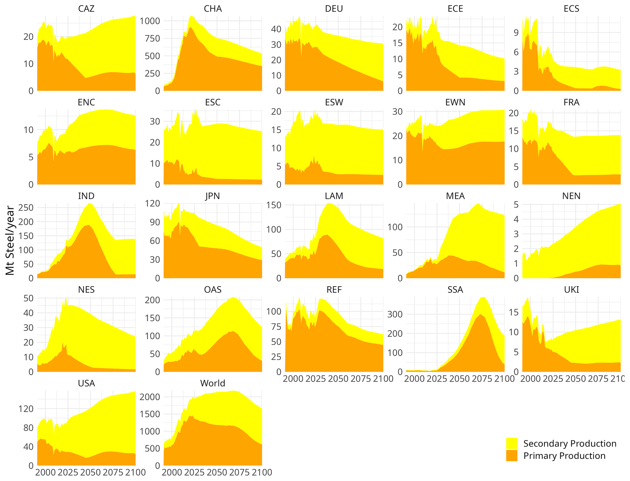
Steel demand adjusted for trade is served by secondary production first, subject to a scrap availability constraint (share of recyclable steel from the deprecated steel stock) and a constraint on the maximum (minimum) share of secondary (primary) steel production, as we assume secondary production to be cheaper than primary production. The remainder of total production is then primary production. The maximum share of secondary steel production is capped at a value that converges linearly from base year levels to the assumed bound of 10 % in 2050, if no region-specific information is used. The reason is twofold: (1) certain applications require high-quality steel that can only be achieved via primary production, and (2) we assume that current production practices and existing production capacity will not change quickly but will continue to be used for economic reasons. Figure 3 shows the historic production (until 2019) and SSP2 projections of primary and secondary steel production.
3.4 Chemical projections
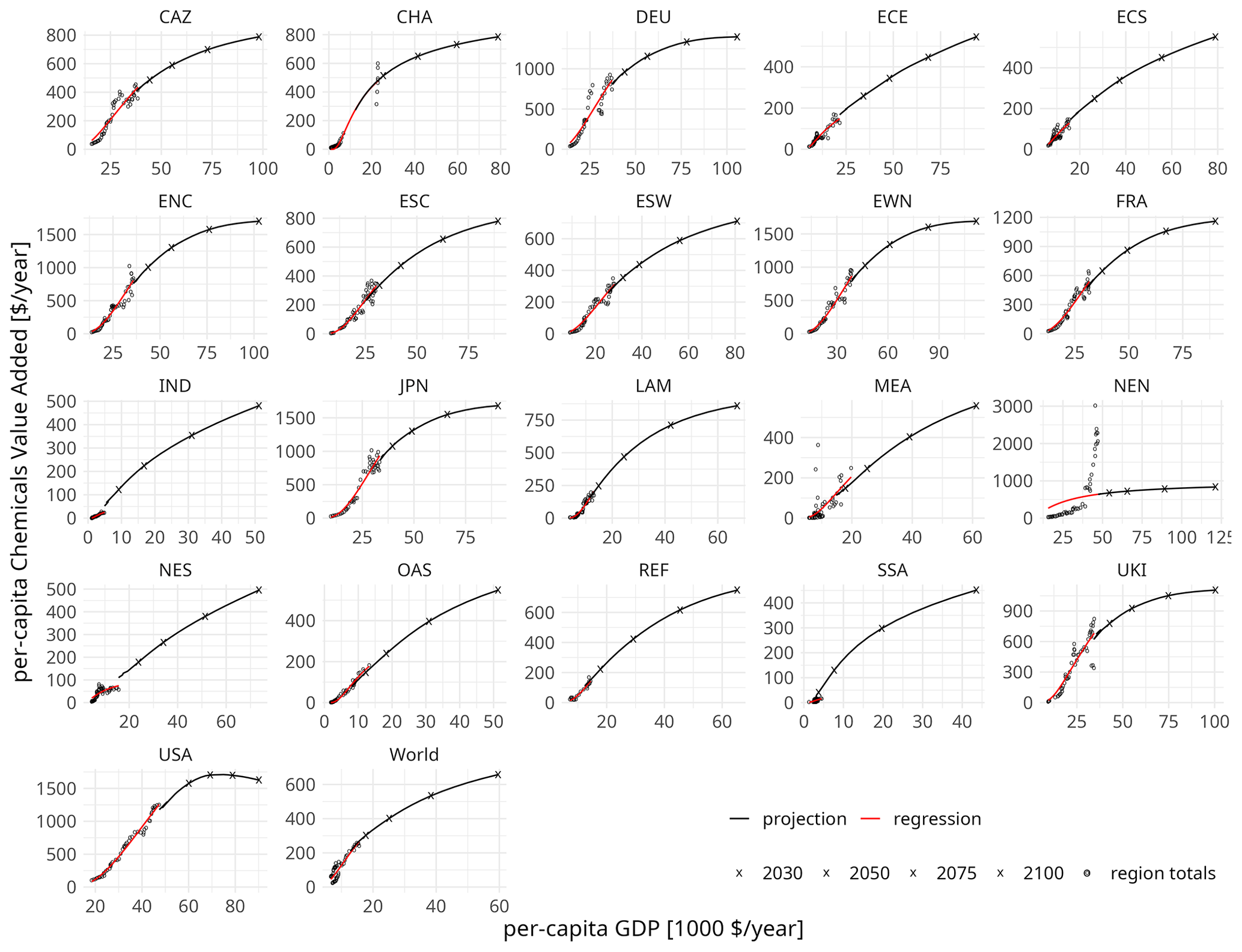
Historic per-capita value added of chemical production is regressed on per-capita GDP using Eq. (3). Chemical value-added data are from the United Nations Industrial Development Organization (2017), ISIC rev. 3 code 24 (chemicals and chemical products); per-capita GDP data are from the World Bank (2019); and population data are from the United Nations Department of Economic and Social Affairs Population Division (2015). Regression parameters are derived once on the regional level and once again on the global level, and regional asymptotes are converged linearly towards the global ones by 2200. Projections of per-capita chemical value added and total chemical value added are calculated from the converged regression parameters (see above) and per-capita GDP and population projections for the SSP2 scenario, respectively. Figure 4 shows the chemical regression data (regionally aggregated), the regression function, and the SSP2 projection of chemical value added.
3.5 Other industry projections
Projecting the activity (value added) of the other industry subsector entails projecting the value added of industry as a whole and subtracting the value added of the three subsectors that are modelled explicitly. To this end, per-capita value added of the entire industry sector is regressed on per-capita GDP using Eq. (3). Industry value-added data are from the United Nations Industrial Development Organization (2017), using ISIC rev. 3 code D “total manufacturing” and table code 20 “value added”; per-capita GDP data are from the World Bank (2019); and population data are from the United Nations Department of Economic and Social Affairs Population Division (2015). Regression parameters are derived once on the regional level and once again on the global level, and regional asymptotes are converged linearly towards the global ones by 2200. Figure 5 shows industry value-added regression data (regionally aggregated), the regression function, and the value-added projections.
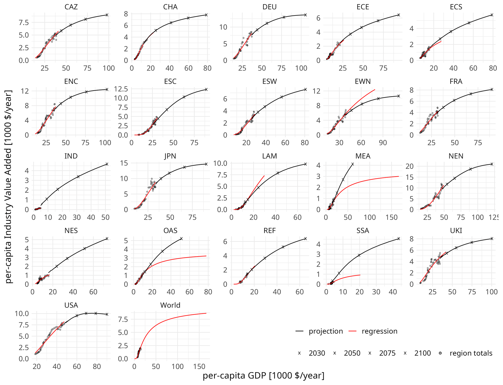
Figure 5Regression and projection of total industry value added. Per-capita industry value added over per-capita GDP for 21 REMIND regions (see Appendix A).
Specific value added of cement and steel production (USD value added per tonne of physical production) is regressed on per-capita GDP using Eq. (3). Cement and steel value-added data are from the United Nations Industrial Development Organization (2017), ISIC rev. 3 codes 26 “non-metallic mineral products” (cement) and 27 “basic metals” (steel), respectively, and table code 20 “value added”. Cement production data are from van Ruijven et al. (2016) and Bas J. van Ruijven (personal communication, 2017); steel production data are from the World Steel Association (2018). Regression parameters are derived on the regional and global levels, and regional asymptotes are converged linearly towards the global level by 2200. Using the converged regression parameters for cement- and steel-specific value added and the projected production of cement and steel, (total) value added of cement and steel production is projected. Figures 6 and 7 show the specific cement and steel regression data (regionally aggregated), the regression functions, and the value-added projections.
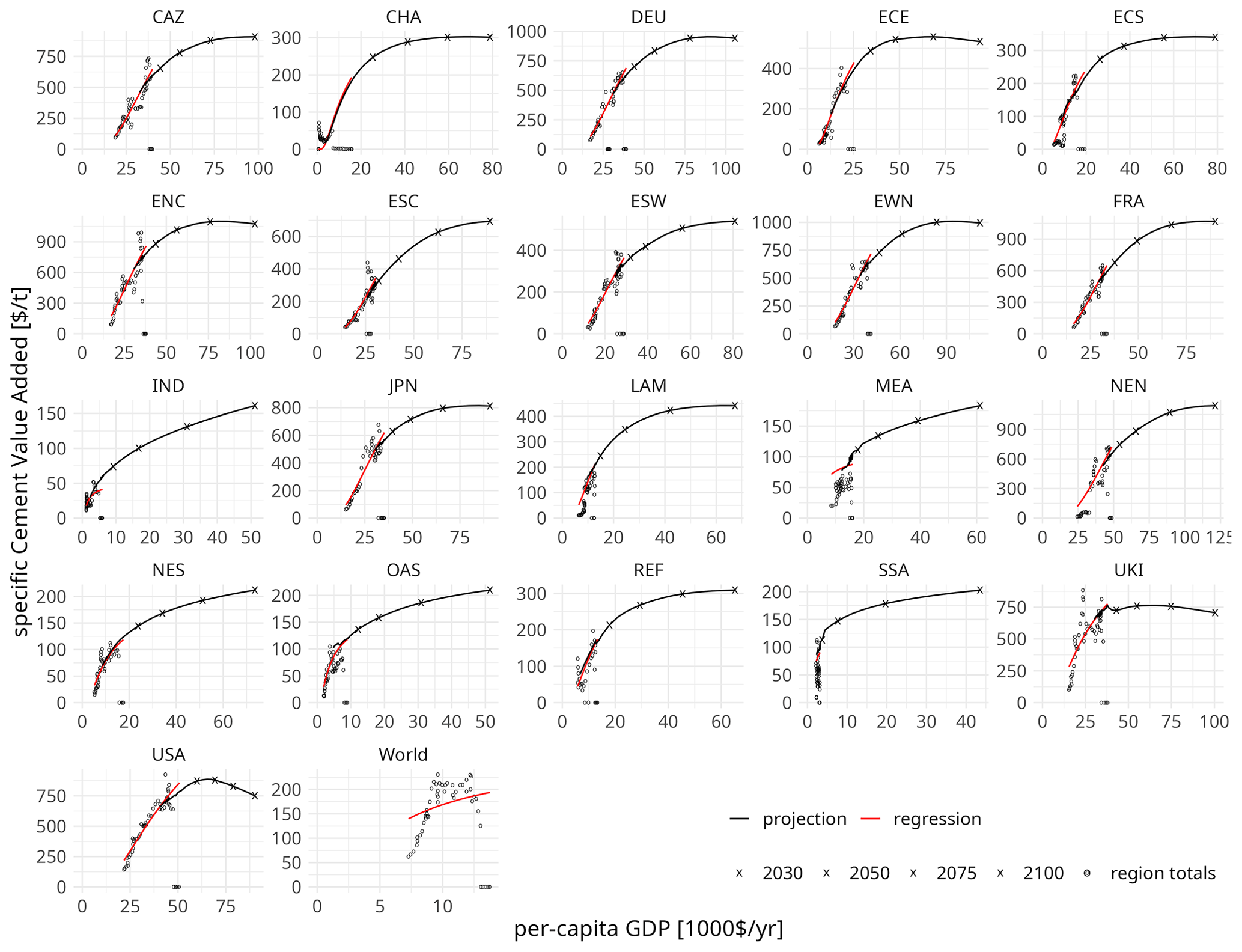
Figure 6Regression and projection of specific cement value added. Per-tonne cement value added over per-capita GDP for 21 REMIND regions (see Appendix A).
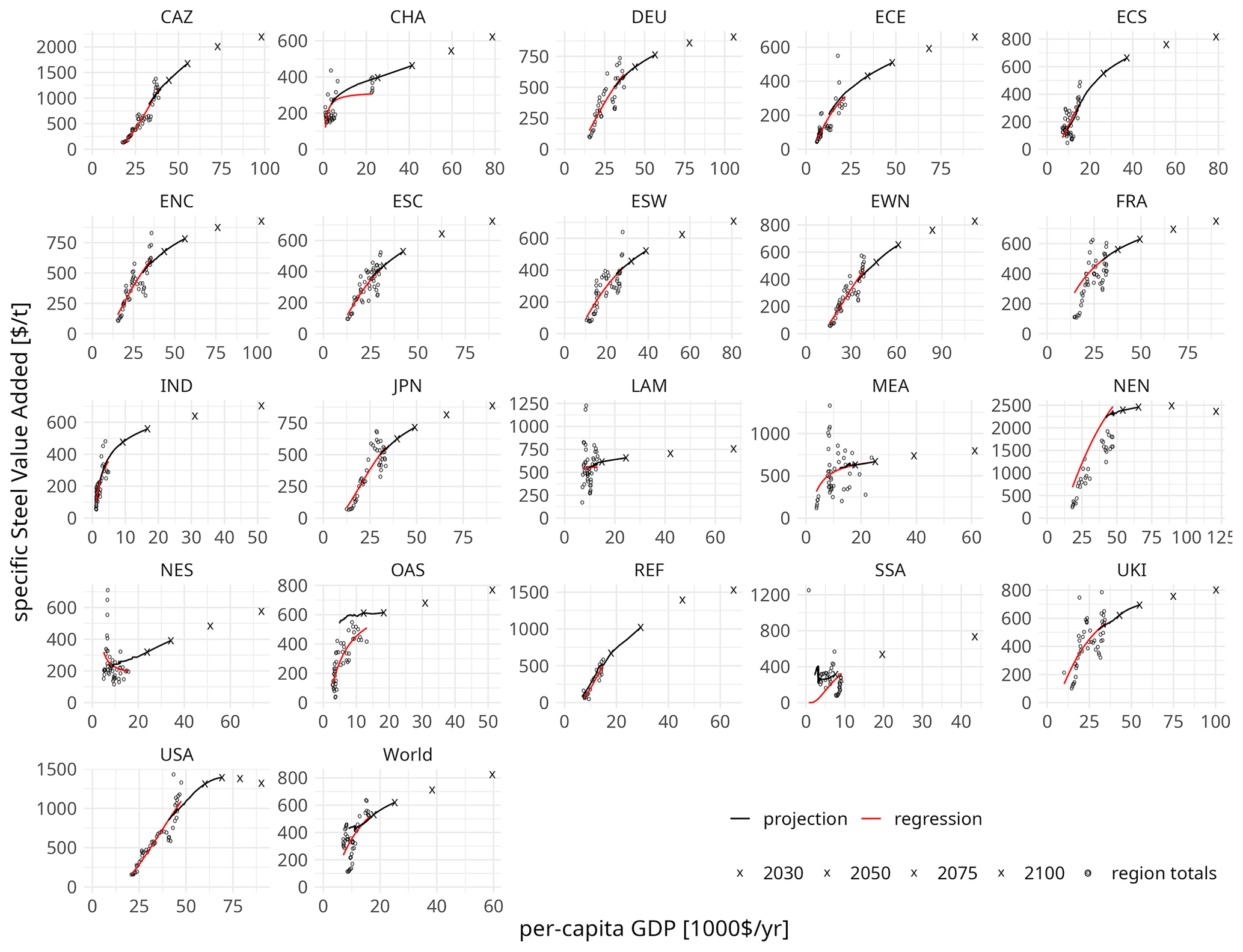
Figure 7Regression and projection of specific steel value added. Per-tonne steel value added over per-capita GDP for 21 REMIND regions (see Appendix A).
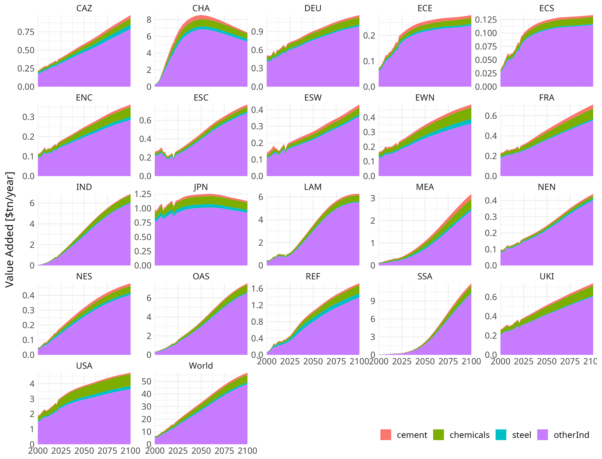
Lastly, projected value added of cement, chemical, and steel production is subtracted from projected value added of the entire industry sector to yield projected value added of the other industry subsector. Figure 8 shows the absolute value added of all four industry subsectors for the SSP2 scenario.
3.6 Final energy projections
Demand of final energy is projected using annual autonomous energy efficiency improvements (Kermeli et al., 2014) that decrease the total (i.e. across energy carriers) specific final energy demand (joule per unit of production or per unit value added) towards a lower bound and by converging the shares of different final energy carriers in total specific final energy demand from historic values towards those of the International Energy Agency (2017) in 2060 (and keeping them constant afterwards). Total (subsector) specific final energy demand is calculated according to the following formula:
where E is the final energy demand, A the activity level (physical production or value added), L the lower limit of specific final energy demand, α the annual autonomous energy efficiency improvement, and t0 the base year. The annual autonomous energy efficiency improvements are chosen such that the overall industry final energy demand trajectories conform to scenario assumptions by other groups (International Energy Agency, 2017). The limit L is set at 1.8 GJ t−1 for cement (Madlool et al., 2011), 8 and 1.3 GJ t−1 for primary and secondary steel (Fruehan et al., 2000), and 10 % of the base year value of the region with the lowest specific energy demand (final energy per value added) for the chemical and other industry subsectors. Table 2 summarises the parameters for the specific final energy demand projections.
Madlool et al. (2011)Fruehan et al. (2000)Fruehan et al. (2000)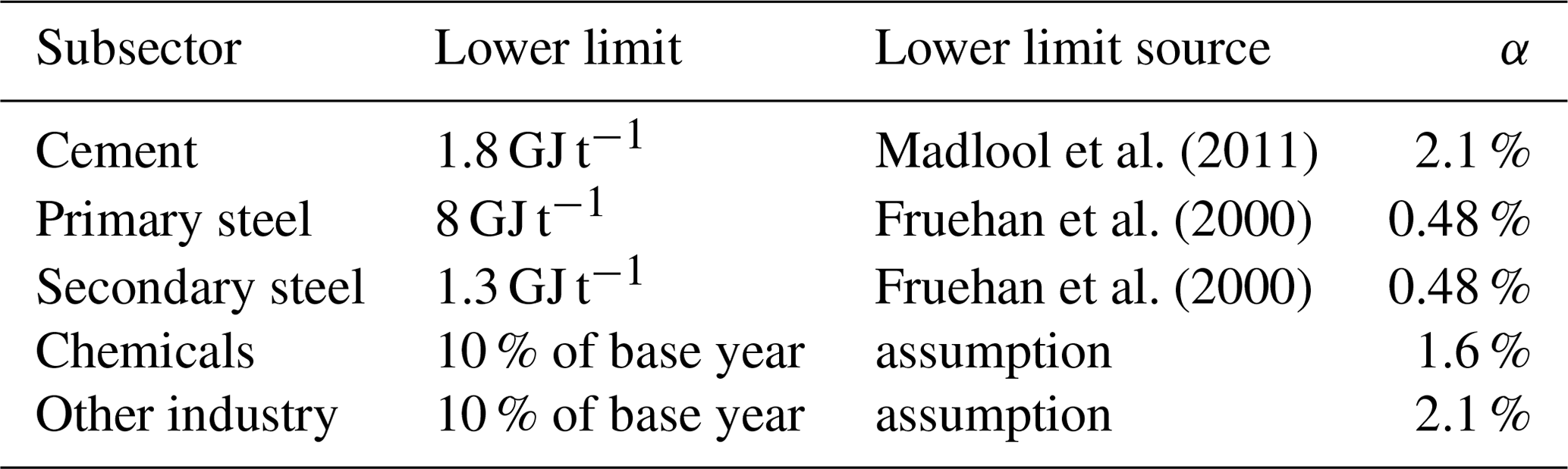
3.7 Scenario variations
Other scenarios are derived from the SSP2 scenario by varying specific material demand (subsector production A per unit GDP) and specific energy demand (joule per unit subsector production). Three methods for varying specific material demand are used: “fixed ratios”, “declining improvements”, and “modified rate of change”, which calculate the scenarios' specific material demand by multiplying either the specific material demand of a reference scenario R (fixed ratios and declining improvements) or the specific material demand of base year t0 (modified rate of change, base year specific material demand is identical across scenarios) with a factor α(t), which is derived differently for the three methods.
Under the fixed ratio method, specific material demand is set to a specific ratio α0 of the specific material demand of the reference scenario R (e.g. cement demand per unit GDP can be set to 95 % of specific cement demand in the reference scenario). The actual parameter α(t) is converged from one to α0 over a time period TC (15 years) from the base year t0 onward.
Under the declining improvement method, annual improvements of specific material demand are assumed, which converge from α0 (e.g. 0.5 % per annum decrease of cement demand per unit GDP) to 0 over the configurable time period TC from base year t0 onward (to preclude exponential decay of the specific demand towards 0). The parameter α(t) is the product of the converged α0 parameter from the base year to year t or one before the base year.
Under the modified rates of change method, relative differences in specific material demand (with respect to the base year t0) of the reference scenario R are either improved (reductions are turned into higher reductions, increases are turned into lower increases) or degraded (increases are turned into higher increases, reductions are turned into lower reductions). To this end, the relative difference β(t) of specific material demand of the reference scenario R, relative to the base year t0,
is multiplied by some factor α0 if the difference is positive (increasing specific demand) or divided by α0 if the difference is negative (decreasing specific demand) to calculate the modified relative difference α(t)
and the specific material demand of scenario S is calculated using base year specific material demand and these modified relative differences,
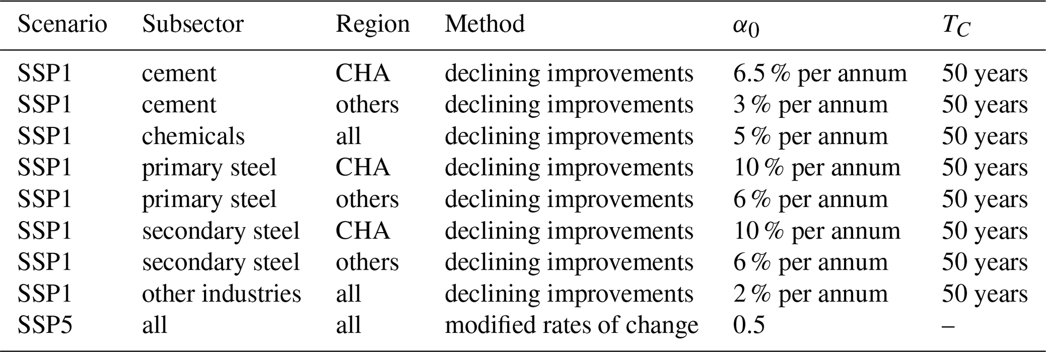
The method of calculating specific material demand and the α0 parameters (and TC in the case of declining improvements) can be chosen individually for combinations of scenarios, regions, and industry subsectors. Table 3 summarises the settings used to derive the SSP1 and SSP5 scenarios from the SSP2 scenario.
Table 3Parameters for deriving the SSP1 and SSP5 scenarios from the SSP2 scenario.
This section exemplifies industry subsector results from the REMIND model for different scenarios. We examine the three socioeconomic baselines SSP1, SSP2, and SSP5 and combine them with three different policy scenarios. The baseline scenarios (base) reproduce the basic SSP scenario narratives without any climate change mitigation policies and are identical to the calibration data derived as described in Sect. 3. The two mitigation scenarios use carbon price trajectories that result in cumulated GHG emissions (i.e. the carbon budget) from 2020 onward to peak at 1150 and 500 Gt CO2 equivalent (“PkBudg1150” and “PkBudg500”) and subsequently decline through net-negative emissions, which are consistent with two possible interpretations of the climate targets of the Paris Accord (limiting global warming to 2 °C with 67 % likelihood or to 1.5 °C with 50 % likelihood; see Arias et al. (2021), Table TS.3).
Figure 9 shows industry subsector activity, indexed to the year 2015. We observe differentiated demand reactions to climate policy across the socioeconomic baselines, the policy scenarios, and between different industry subsectors.
In accordance with the SSP scenario narratives (Bauer et al., 2017; O'Neill et al., 2017) (see Sect. 3.7), the SSP1 base scenario shows lower growth in industry demand (−30 % to 210 %, 2015 to 2100 change) than the SSP2 scenario (−47 % to 360 %), while the SSP5 base scenario shows higher growth (140 % to 810 %), reproducing the data from the projection and scenario variation steps (Sect. 3). The other industry subsector sees the highest growth across all socioeconomic baselines (210 % to 810 %), in line with the assumed increase in the share of industries producing high-value goods as opposed to bulk materials. The increase in the chemical subsector's activity (46 % to 690 %) also agrees with the assumption of higher shares of products from light metals like aluminium, plastics, and other modern materials rather than steel.
For all socioeconomic baselines, we see a reduction in industry demand with strengthened climate targets (reduced budgets for further GHG emissions), as well as a shift from primary (−47 % to 140 %) to secondary steel (4 % to 610 %), since the latter is produced from electricity which is easier to produce carbon-free.
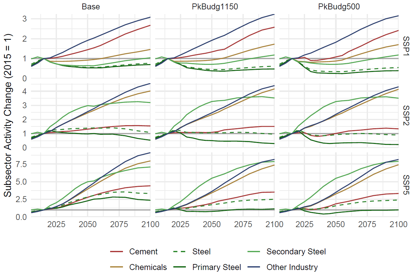
Figure 9Industry subsector activity change. Production of cement and primary and secondary steel, as well as chemicals and other industry value added, indexed to 2015. Panels correspond to the scenario matrix, with socioeconomic drivers (SSP1, SSP2, SSP5) and climate change mitigation policy (base – no policy, PkBudg1150 and PkBudg500 – peak budgets of 1150 and 500 Gt CO2, corresponding to the 2 and 1.5 °C targets).
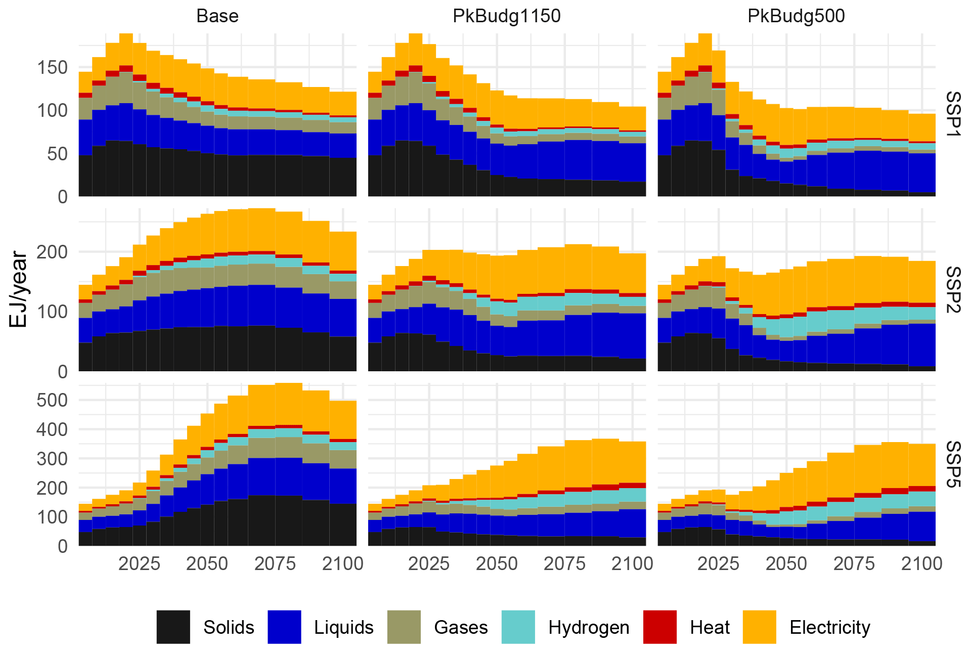
Figure 10Industry final energy demand by energy carrier. Panels correspond to the scenario matrix, with socioeconomic drivers (SSP1, SSP2, SSP5) and climate change mitigation policy (base – no policy, PkBudg1150 and PkBudg500 – peak budgets of 1150 and 500 Gt CO2, corresponding to the 2 and 1.5 °C targets). Solids, liquids, and gases combine final energy carriers from fossil and non-fossil sources.
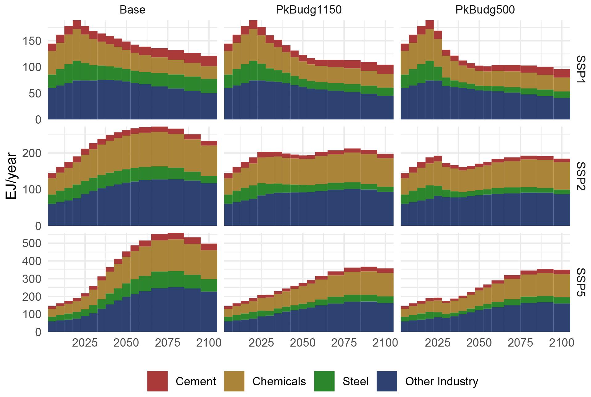
Figure 11Industry subsector final energy demand. Panels correspond to the scenario matrix, with socioeconomic drivers (SSP1, SSP2, SSP5) and climate change mitigation policy (base – no policy, PkBudg1150 and PkBudg500 – peak budgets of 1150 and 500 Gt CO2, corresponding to the 2 and 1.5 °C targets).
Figures 10 and 11 show industry final energy (FE) demand, by subsector and energy carrier. Both the shares of individual energy carriers and of the different subsectors vary across the scenario matrix, as the model reacts differently to the emission constraints in the different socioeconomic baselines.
For a comparison of total industry FE demand with historic data and other projections, see Appendix B. Total FE demand of the SSP2 scenario increases in accordance with the “reference technology scenario” from the International Energy Agency (2017) until 2050 (see Sect. 3.6), with SSP1 and SSP5 markedly higher and lower, respectively.
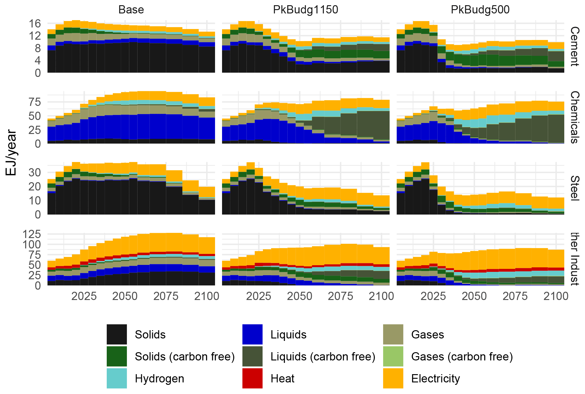
Figure 12Industry final energy demand by subsector and energy carrier for the SSP2 scenario. Solids, liquids, and gases derived from either biomass or (renewable) hydrogen are grouped under carbon-free.
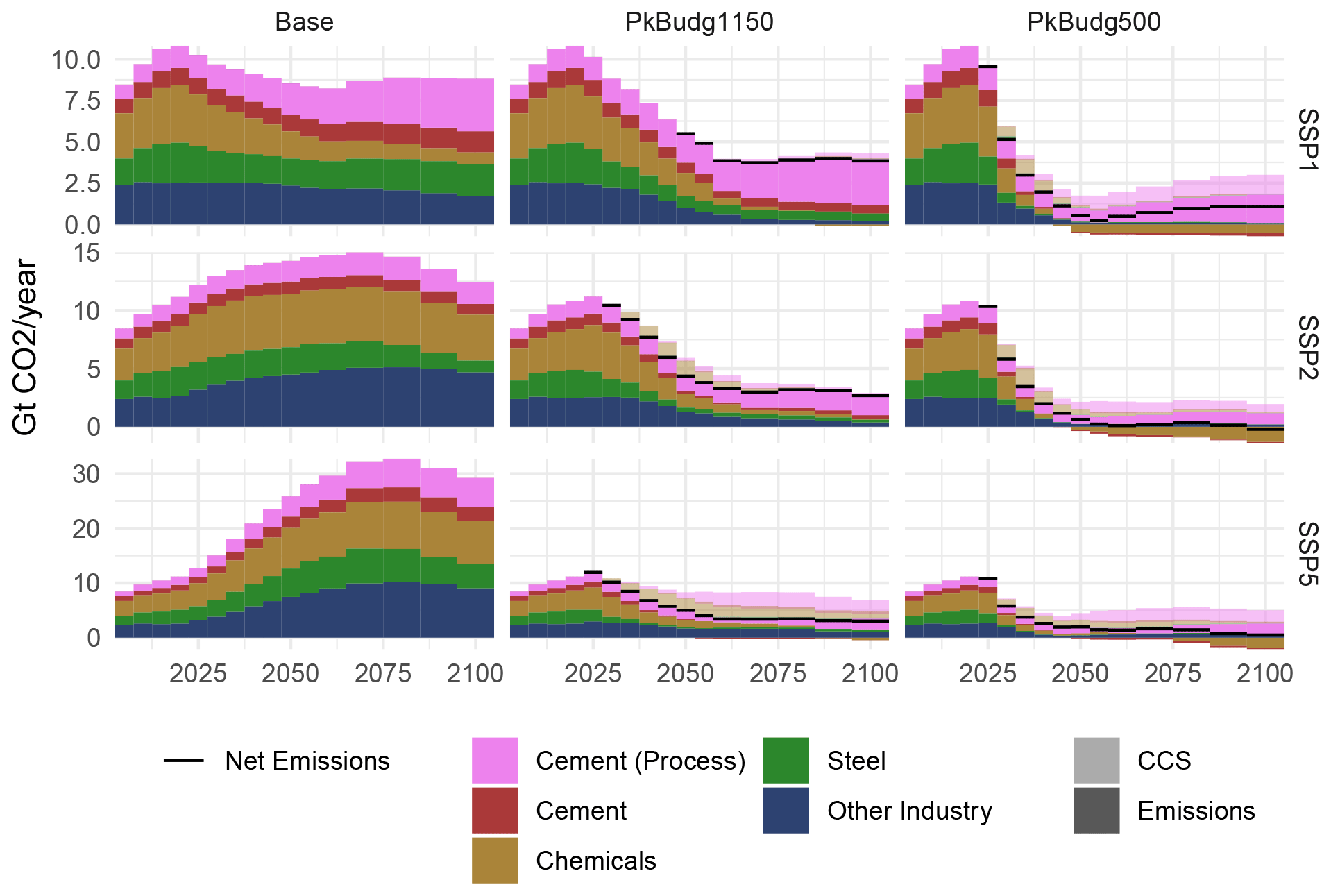
Figure 13Industry CO2 emissions and CCS. Net emissions are shown for periods with CCS or negative emissions (through bioenergy and CCS). Panels correspond to the scenario matrix, with socioeconomic drivers (SSP1, SSP2, SSP5) and climate change mitigation policy (base – no policy, PkBudg1150 and PkBudg500 – peak budgets of 1150 and 500 Gt CO2, corresponding to the 2 and 1.5 °C targets).
The SSP1 base scenario shows an immediate decline in industry FE demand, in accordance with the scenario narrative of sustainability and efficiency, while the SSP2 and SSP5 scenarios display an increase and subsequent decrease in FE demand, albeit to markedly different levels (273 EJ yr−1 peak in 2070 for SSP2 and 559 EJ yr−1 peak in 2080 for SSP5). The share of electricity (an indicator of industry decarbonisation) rises to 28 % in 2090 for the base scenarios and 45 %–49 % in 2080 (PkBudg1150) and 2055 (PkBudg500) for the mitigation scenarios, while the share of solids decreases strongly, to be partially replaced with liquid final energy carriers, part of which will be generated from biomass.
Figure 12 exemplifies the differences in mitigation strategies of the industry subsectors for the set of SSP2 scenarios. The cement and chemical subsectors, which cannot easily electrify, move to carbon-free fuels either directly in the from of biomass or hydrogen or indirectly by using hydrogen-derived synthetic fuels (biomass and synthetic fuel are grouped under carbon-free). The steel sector decarbonises by expanding production of secondary steel that uses carbon-free electricity (within the limits of scrap availability), by reducing production of primary steel and by switching to carbon-free fuels. The other industry subsector substitutes electricity for fuels while also increasing energy efficiency, so the total electricity demand increases only slightly and moves to carbon-free fuels. Notably, the residual share of fossil fuels is the lowest in the other industry subsector, as it does not allow for the application of CCS.
Figure 13 shows industry CO2 emissions and CCS by industry subsector. The emissions in the baseline scenarios follow the trajectory of the total demand in final energy of fossil origin (see solids, liquids, and gases in Fig. 10), while their composition differs from the subsector composition of FE demand (see Fig. 11, as the other industry subsector moves to higher shares of electricity in FE demand, while the heavy-industry subsectors rely more strongly on fossil fuels for high-temperature heat generation. Process emissions from cement production become a dominant fraction, as they are fixed relative to cement production and thus do not benefit from energy efficiency improvements, and cement production expands (especially in emerging economies). The electrification trend is intensified in the climate mitigation scenarios and complemented by CCS to mitigate emissions from fossil fuels in the heavy-industry subsectors that cannot be substituted (cement and chemicals), while the use of biomass fuels combined with CCS can even yield negative emissions in strong decarbonisation scenarios.
As industry is a key contributor to GHG emissions and faces particular mitigation challenges compared to other energy demand sectors and the energy supply sector, it has to be considered both in detail and in conjunction with the entire system of macroeconomic production, energy demand, and carbon management options. The differentiation of the main industry subsectors enables the REMIND model to represent their different mitigation options and challenges in detail while keeping them linked to the other economic sectors and the energy supply system, as well as the emissions, CCS, and CDR submodels, thus allowing for a consistent analysis of the entire energy–economy–climate system.
The projection of baseline scenarios of industry activity, energy demand, and CO2 emissions is a prerequisite for developing and exploring climate change mitigation scenarios. The presented approach allows for both the generation of trajectories that replicate short-term trends and long-term global convergence of specific activity and ways to conveniently and transparently modify these long-term trends to enable the creation of scenarios with different narratives to explore, like the different SSP scenarios.
The resulting REMIND model (in different stages of refinement) and scenarios were (e.g. Luderer et al., 2022) and are currently (e.g. Schreyer et al., 2024; Bauer et al., 2024) used to investigate industry mitigation options and their implications for other economic sectors and the economy as a whole. A detailed analysis of industry subsector mitigation options and challenges that takes full advantage of these new modelling facilities is in preparation. It aims to spell out in detail the different drivers of emissions and their mitigation options and to identify crucial bottlenecks for reducing the unavoidable residual GHG emissions from industry that will have to be offset by CDR measures.
Possible future extensions include the integration of material flow analysis to improve the representation of the physical characteristics of different industry subsectors (e.g. an endogenous representation of in-use stocks of steel and plastics and their lifetimes as a limitation to their recycling, which are not captured well by the CES formulation), the introduction of feedbacks between other economic sectors and the demand for industry products (e.g. shrinking demand for steel through light-weighting of cars or the use of timber or carbon fibres instead of steel-reinforced concrete in construction), the effect of cheap variable electricity from renewables on direct and indirect (through hydrogen) electrification of industry, and international trade in energy-intensive industrial goods and a subsequent shift in production patterns of industry towards world regions with cheap abundant energy.
The 21 region configuration for REMIND used to derive industry activity and final energy trajectories is comprised of regions with individual large countries (China – CHA, India – IND, Japan – JPN, and the United States of America – USA), country groups (Canada, Australia, New Zealand – CAZ, Latin America – LAM, the Middle East and northern Africa – MEA, other Asia – OAS, the former Soviet Union – REF, and sub-Saharan Africa – SSA), and countries and country groups dividing Europe in roughly equal-sized regions that are EU members (DEU, ECE, ECS, ENC, ESC, ESW, EWN, and FRA) or not (NEN, NES, and UKI, with Ireland being grouped with the United Kingdom even though the former is an EU member).
Table A1 lists the 21 regions and the countries grouped under them.
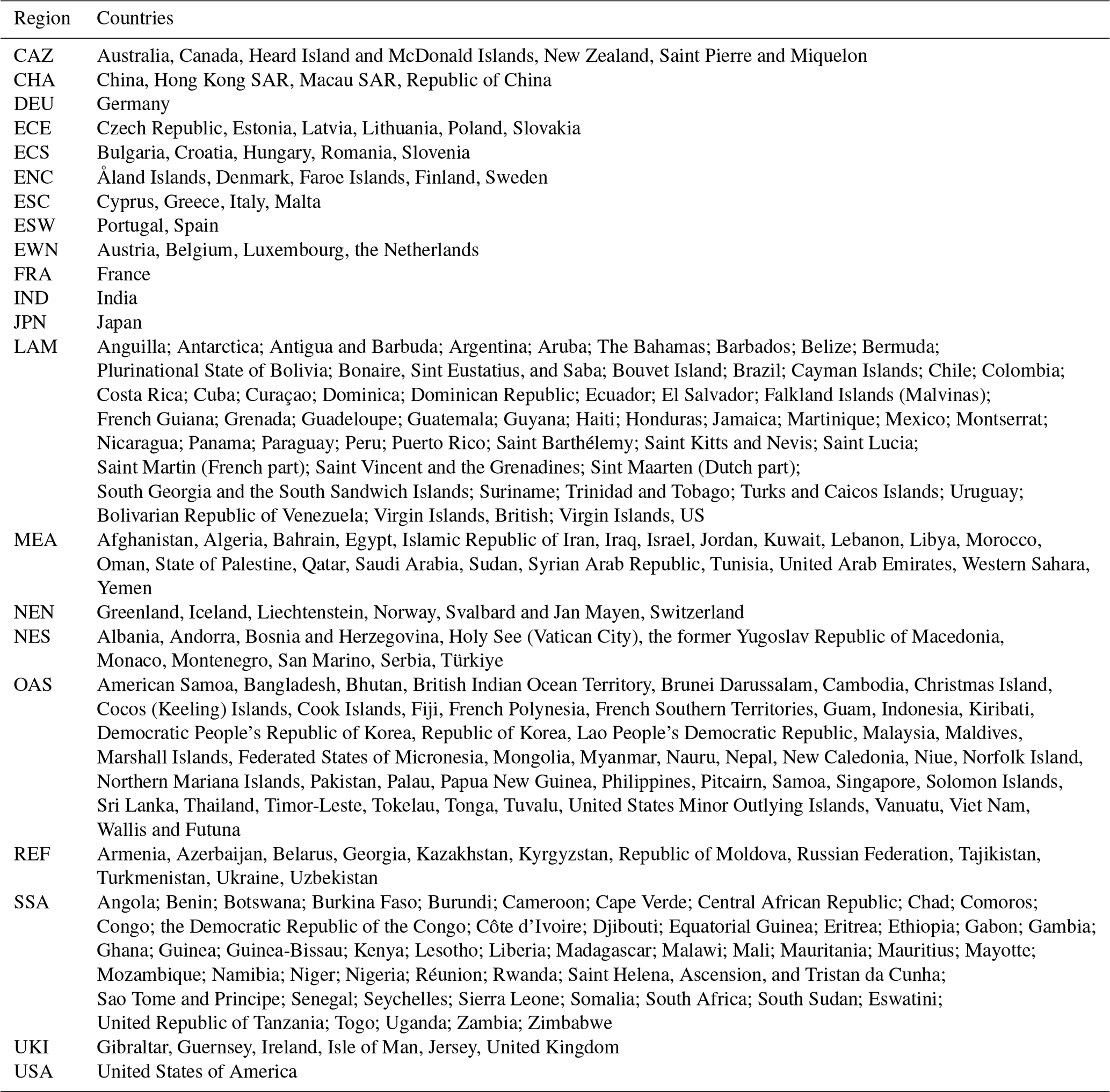
Figure B1 shows a comparison of industry final energy demand by energy carrier for the three baseline scenarios (SSP1, SSP2, and SSP5) with recent historic data (2000–2020, from the International Energy Agency (2022)) as well as two exemplary scenarios for near-term (until 2050) industry final energy demand, the “announced pledge scenario” (APS; International Energy Agency (2021)), and the “reference technology scenario” (RTS; International Energy Agency (2017)).
Note that all three sources (although stemming from the same source) differ in the way final energy carriers are aggregated and whether agriculture, fisheries, forestry, and refineries are included with industry or not.
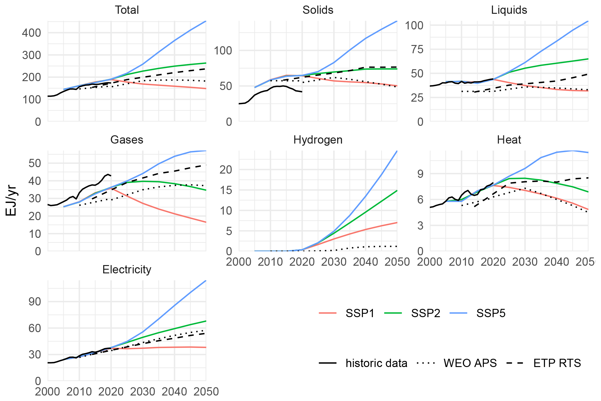
Figure B1Comparison of industry final energy demand for the SSP1, SSP2, and SSP5 baseline scenarios to historic data (derived from the International Energy Agency, 2022), the announced pledge scenario (APS) from the International Energy Agency (2021), and the reference technology scenario (RTS) from the International Energy Agency (2017).
The REMIND model is written in GAMS, with supporting scripts in R, and version 3.1.0 of the model is archived in Zenodo (https://doi.org/10.5281/zenodo.7628336, Luderer et al., 2023).
The code for preparing the REMIND input data is written in R, and version 0.165.6 of the principal package mrremind is available at Zenodo (https://doi.org/10.5281/zenodo.10495588, Baumstark et al., 2024).
The data used for preparing the REMIND input data are partly proprietary and only available upon request.
The source of this paper, including the R code for preparing the figures, is available at Zenodo (https://doi.org/10.5281/zenodo.8272197, Pehl, 2024). It is, however, not fully functioning as one proprietary data source (UNIDO INSTAT) cannot be shared publicly and had to be redacted.
MP and GL designed the industry subsector formulation and scenario generation, which were implemented by MP. The mark-up costs for hydrogen and high-temperature electricity were developed by FS. The paper was written by MP with input from all authors. All work was supervised by GL.
The contact author has declared that none of the authors has any competing interests.
Publisher's note: Copernicus Publications remains neutral with regard to jurisdictional claims made in the text, published maps, institutional affiliations, or any other geographical representation in this paper. While Copernicus Publications makes every effort to include appropriate place names, the final responsibility lies with the authors.
The research leading to these results has received funding from the German Federal Ministry of Education and Research under grant agreement no. 03SFK5A (Ariadne) and the European Union's Horizon 2020 research and innovation programme under grant agreement no. 101022622 (ECEMF).
This research has been supported by the German Federal Ministry of Education and Research (grant no. 03SFK5A (Ariadne)) and the European Union's Horizon 2020 (grant no. 101022622 (ECEMF)).
The article processing charges for this open-access publication were covered by the Potsdam Institute for Climate Impact Research (PIK).
This paper was edited by Sam Rabin and reviewed by two anonymous referees.
Arias, P. A., Bellouin, N., Coppola, E., Jones, R. G., Krinner, G., Marotzke, J., Naik, V., Palmer, M. D., Plattner, G.-K., Rogelj, J., Rojas, M., Sillmann, J., Storelvmo, T., Thorne, P. W., Trewin, B., Achuta Rao, K., Adhikary, B., Allan, R. P., Armour, K., Bala, G., Barimalala, R., Berger, S., Canadell, J. G., Cassou, C., Cherchi, A., Collins, W., Collins, W. D., Connors, S. L., Corti, S., Cruz, F., Dentener, F. J., Dereczynski, C., Di Luca, A., Diongue Niang, A., Doblas-Reyes, F. J., Dosio, A., Douville, H., Engelbrecht, F., Eyring, V., Fischer, E., Forster, P., Fox-Kemper, B., Fuglestvedt, J. S., Fyfe, J. C., Gillett, N. P., Goldfarb, L., Gorodetskaya, I., Gutierrez, J. M., Hamdi, R., Hawkins, E., Hewitt, H. T., Hope, P., Islam, A. S., Jones, C., Kaufman, D. S., Kopp, R. E., Kosaka, Y., Kossin, J., Krakovska, S., Lee, J.-Y., Li, J., Mauritsen, T., Maycock, T. K., Meinshausen, M., Min, S.-K., Monteiro, P. M. S., Ngo-Duc, T., Otto, F., Pinto, I., Pirani, A., Raghavan, K., Ranasinghe, R., Ruane, A. C., Ruiz, L., Sallée, J.-B., Samset, B. H., Sathyendranath, S., Seneviratne, S. I., Sörensson, A. A., Szopa, S., Takayabu, I., Tréguier, A.-M., van den Hurk, B., Vautard, R., von Schuckmann, K., Zaehle, S., Zhang, X., and Zickfeld, K.: Technical Summary, in: Climate Change 2021: The Physical Science Basis. Contribution of Working Group I to the Sixth Assessment Report of the Intergovernmental Panel on Climate Change, 33–144, Cambirdge University Press, Cambridge, United Kingdom and New York, NY, USA, ISBN 978-92-9169-160-9, 2021. a, b
Arujo, E., Bodirsky, B. L., Crawford, M. S., Leip, D., and Dietrich, J.: MissingIslands Dataset for Filling in Data Gaps from the WDI Datasets, Zenodo [data set], https://doi.org/10.5281/zenodo.4421504, 2021. a, b
Bashmakov, I., Nilsson, L., Acquaye, A., Bataille, C., Cullen, J., S. de la Rue du Can, Fischedick, M., Geng, Y., and Tanaka, K.: Industry, in: Climate Change 2022: Mitigation of Climate Change. Contribution of Working Group III to the Sixth Assessment Report of the Intergovernmental Panel on Climate Change, 1161–1243, Cambridge University Press, Cambridge, UK and New York, NY, US, ISBN 978-92-9169-160-9, 2022. a, b, c
Bauer, N., Calvin, K., Emmerling, J., Fricko, O., Fujimori, S., Hilaire, J., Eom, J., Krey, V., Kriegler, E., Mouratiadou, I., de Boer, H. S., van den Berg, M., Carrara, S., Daioglou, V., Drouet, L., Edmonds, J. E., Gernaat, D., Havlik, P., Johnson, N., Klein, D., Kyle, P., Marangoni, G., Masui, T., Pietzcker, R. C., Strubegger, M., Wise, M., Riahi, K., and van Vuuren, D. P.: Shared Socio-Economic Pathways of the Energy Sector – Quantifying the Narratives, Global Environ. Change, 42, 316–330, https://doi.org/10.1016/j.gloenvcha.2016.07.006, 2017. a
Bauer, N., Moreno, S., de Boer, H.-S., Fragkiadakis, D., Fragkos, P., Keramidas, K., van Sluisfeld, M., Unlu, G., Zotin, M., Baptista, L. B., Benke, F., Fragkiadakis, K., Krey, V., Luderer, G., Maczek, F., Madeddu, S., Min, J., Pehl, M., Rochedo, P., and van Vuuren, D.: Integrated Strategies Minimize Hard-to-Abate Industry Sector CO2 Emissions in Low-Emission Scenarios, in preparation, 2024. a, b, c
Baumstark, L., Bauer, N., Benke, F., Bertram, C., Bi, S., Gong, C. C., Dietrich, J. P., Dirnaichner, A., Giannousakis, A., Hilaire, J., Klein, D., Koch, J., Leimbach, M., Levesque, A., Madeddu, S., Malik, A., Merfort, A., Merfort, L., Odenweller, A., Pehl, M., Pietzcker, R. C., Piontek, F., Rauner, S., Rodrigues, R., Rottoli, M., Schreyer, F., Schultes, A., Soergel, B., Soergel, D., Strefler, J., Ueckerdt, F., Kriegler, E., and Luderer, G.: REMIND2.1: transformation and innovation dynamics of the energy-economic system within climate and sustainability limits, Geosci. Model Dev., 14, 6571–6603, https://doi.org/10.5194/gmd-14-6571-2021, 2021. a, b, c
Baumstark, L., Rodrigues, R., Levesque, A., Oeser, J., Bertram, C., Mouratiadou, I., Malik, A., Schreyer, F., Soergel, B., Rottoli, M., Mishra, A., Dirnaichner, A., Pehl, M., Giannousakis, A., Klein, D., Strefler, J., Feldhaus, L., Brecha, R., Rauner, S., Dietrich, J. P., Bi, S., Benke, F., Weigmann, P., Richters, O., Hasse, R., Fuchs, S., and Mandaroux, R.: mrremind: MadRat REMIND Input Data Package (v0.165.6), Zenodo [code], https://doi.org/10.5281/zenodo.10495588, 2024. a
Chung, J. W.: Utility and Production Functions: Theory and Applications, Blackwell, Oxford, UK, Cambridge, Mass., USA, ISBN 978-1-55786-417-8, 1994. a
Daehn, K. E., Cabrera Serrenho, A., and Allwood, J. M.: How Will Copper Contamination Constrain Future Global Steel Recycling?, Environ. Sci. Technol., 51, 6599–6606, https://doi.org/10.1021/acs.est.7b00997, 2017. a
Deason, J., Wei, M., Leventis, G., Smith, S., and Schwartz, L.: Electrification of Buildings and Industry in the United States: Drivers, Barriers, Prospects, and Policy Approaches, Tech. rep., Ernest Orlando Lawrence Berkeley National Laboratory, Berkeley, California, USA, 2018. a
Després, J., Keramidas, K., Schmitz, A., Kitous, A., Schade, B., Diaz Vazquez, A., Mima, S., Russ, H. P., and Wiesenthal, T.: POLES-JRC Model Documentation: 2018 Update, Tech. Rep. JRC113757, European Commission, Joint Research Centre, Luxembourg, 2018. a
Fischedick, M., Roy, J., Abdel-Aziz, A., Acquaye, A., Allwood, J., Ceron, J.-P., Geng, Y., Kheshgi, H., Lanza, A., Perczyk, D., Price, L., Santalla, E., Sheinbaum, C., and Tanaka, K.: Industry, in: Climate Change 2014: Mitigation of Climate Change. Contribution of Working Group III to the Fifth Assessment Report of the Intergovernmental Panel on Climate Change, edited by: Edenhofer, O., Pichs-Madruga, R., Sokona, Y., Farahani, E., Kadner, S., Seyboth, K., Adler, A., Baum, I., Brunner, S., Eickemeier, P., Kriemann, B., Savolainen, J., Schlömer, S., von Stechow, C., Zwickel, T., and Minx, J. C., Cambirdge University Press, Cambridge, United Kingdom and New York, NY, USA, 2014. a, b, c, d
Fragkos, P. and Fragkiadakis, K.: Analyzing the Macro-Economic and Employment Implications of Ambitious Mitigation Pathways and Carbon Pricing, Front. Climate, 4, https://doi.org/10.3389/fclim.2022.785136, 2022. a
Fragkos, P., Kouvaritakis, N., and Capros, P.: Incorporating Uncertainty into World Energy Modelling: The PROMETHEUS Model, Environ. Model. A., 20, 549–569, https://doi.org/10.1007/s10666-015-9442-x, 2015. a
Fruehan, R., Fortini, O., Paxton, H., and Brindle, R.: Theoretical Minimum Energies to Produce Steel for Selected Conditions, Tech. Rep. NONE, 769470, https://doi.org/10.2172/769470, 2000. a, b, c
Fuss, S., Lamb, W. F., Callaghan, M. W., Hilaire, J., Creutzig, F., Amann, T., Tim Beringer, Garcia, W. d. O., Hartmann, J., Khanna, T., Luderer, G., Nemet, G. F., Joeri Rogelj, Smith, P., Vicente, J. L. V., Wilcox, J., Dominguez, M. d. M. Z., and Minx, J. C.: Negative Emissions – Part 2: Costs, Potentials and Side Effects, Environ. Res. Lett., 13, 063002, https://doi.org/10.1088/1748-9326/aabf9f, 2018. a
Grubler, A., Wilson, C., Bento, N., Boza-Kiss, B., Krey, V., McCollum, D. L., Rao, N. D., Riahi, K., Rogelj, J., Stercke, S. D., Cullen, J., Frank, S., Fricko, O., Guo, F., Gidden, M., Havlík, P., Huppmann, D., Kiesewetter, G., Rafaj, P., Schoepp, W., and Valin, H.: A Low Energy Demand Scenario for Meeting the 1.5 °C Target and Sustainable Development Goals without Negative Emission Technologies, Nature Energy, 3, 515–527, https://doi.org/10.1038/s41560-018-0172-6, 2018. a
International Energy Agency: World Energy Investment Outlook, Tech. rep., International Energy Agency, Paris, https://www.iea.org/reports/world-energy-investment-outlook (last access: 15 June 2023), 2014. a, b
International Energy Agency: Energy Technology Perspectives 2017: Catalyzing Energy Technology Transformations, Tech. Rep. 2079-259X, International Energy Agency, Paris, edited by: Justus, D. and French-Brooks, J., https://www.iea.org/reports/energy-technology-perspectives-2017 (last access: 23 January 2020), 2017. a, b, c, d, e
International Energy Agency: World Energy Outlook 2021, International Energy Agency, Paris, edited by: Hosker, E., https://www.iea.org/reports/world-energy-outlook-2021, 2021. a, b, c, d
International Energy Agency: World Energy Balances Database, https://www.iea.org/data-and-statistics/data-product/world-energy-balances (last access: 3 August 2022), 2022. a, b
James, S. L., Gubbins, P., Murray, C. J., and Gakidou, E.: Developing a Comprehensive Time Series of GDP per Capita for 210 Countries from 1950 to 2015, Population Health Metrics, 10, 12, https://doi.org/10.1186/1478-7954-10-12, 2012. a, b
Kaya, Y., Yokobori, K., University, U. N., and Conference on Global Environment, Energy, and Economic Development, Environment, Energy, and Economy: Strategies for Sustainability, United Nations Univ. Press, Tokyo, ISBN 978-92-808-0911-4, 1997. a
KC, S. and Lutz, W.: The Human Core of the Shared Socioeconomic Pathways: Population Scenarios by Age, Sex and Level of Education for All Countries to 2100, Global Environ. Change, 42, 181–192, https://doi.org/10.1016/j.gloenvcha.2014.06.004, 2017. a, b, c
Kermeli, K., Graus, W. H. J., and Worrell, E.: Energy Efficiency Improvement Potentials and a Low Energy Demand Scenario for the Global Industrial Sector, Energy Efficiency, 7, 987–1011, https://doi.org/10.1007/s12053-014-9267-5, 2014. a
Kermeli, K., van Ruijven, B., Graus, W.-C., Edelenbosch, O., Worrell, E., and van Vuuren, D.: Enhancing the Representation of Energy Demand Developments in IAM Models – A Modeling Guide for the Cement Industry, Tech. rep., http://fp7-advance.eu/?q=content/industrial-sector-cement-guideline (last access: 7 July 2023), 2016. a
Koch, J. and Leimbach, M.: SSP Economic Growth Projections: Major Changes of Key Drivers in Integrated Assessment Modelling, Ecol. Econ., 206, 107751, https://doi.org/10.1016/j.ecolecon.2023.107751, 2023. a, b, c
Kriegler, E., Bauer, N., Popp, A., Humpenöder, F., Leimbach, M., Strefler, J., Baumstark, L., Bodirsky, B. L., Hilaire, J., Klein, D., Mouratiadou, I., Weindl, I., Bertram, C., Dietrich, J.-P., Luderer, G., Pehl, M., Pietzcker, R., Piontek, F., Lotze-Campen, H., Biewald, A., Bonsch, M., Giannousakis, A., Kreidenweis, U., Müller, C., Rolinski, S., Schultes, A., Schwanitz, J., Stevanovic, M., Calvin, K., Emmerling, J., Fujimori, S., and Edenhofer, O.: Fossil-Fueled Development (SSP5): An Energy and Resource Intensive Scenario for the 21st Century, Global Environ. Change, 42, 297–315, https://doi.org/10.1016/j.gloenvcha.2016.05.015, 2017. a
Kuramochi, T., Ramírez, A., Turkenburg, W., and Faaij, A.: Comparative Assessment of CO2 Capture Technologies for Carbon-Intensive Industrial Processes, Prog. Energ. Combust., 38, 87–112, https://doi.org/10.1016/j.pecs.2011.05.001, 2012. a, b
Luderer, G., Vrontisi, Z., Bertram, C., Edelenbosch, O. Y., Pietzcker, R. C., Rogelj, J., de Boer, H. S., Drouet, L., Emmerling, J., Fricko, O., Fujimori, S., Havlík, P., Iyer, G., Keramidas, K., Kitous, A., Pehl, M., Krey, V., Riahi, K., Saveyn, B., Tavoni, M., van Vuuren, D. P., and Kriegler, E.: Residual Fossil CO2 Emissions in 1.5–2 °C Pathways, Nat. Clim. Change, 8, 626–633, https://doi.org/10.1038/s41558-018-0198-6, 2018. a
Luderer, G., Madeddu, S., Merfort, L., Ueckerdt, F., Pehl, M., Pietzcker, R., Rottoli, M., Schreyer, F., Bauer, N., Baumstark, L., Bertram, C., Dirnaichner, A., Humpenöder, F., Levesque, A., Popp, A., Rodrigues, R., Strefler, J., and Kriegler, E.: Impact of Declining Renewable Energy Costs on Electrification in Low-Emission Scenarios, Nature Energy, 7, 32–42, https://doi.org/10.1038/s41560-021-00937-z, 2022. a, b
Luderer, G., Bauer, N., Baumstark, L., Bertram, C., Leimbach, M., Pietzcker, R., Strefler, J., Aboumahboub, T., Abrahão, G., Auer, C., Benke, F., Bi, S., Dietrich, J., Dirnaichner, A., Führlich, P., Giannousakis, A., Gong, C. C., Haller, M., Hasse, R., Hilaire, J., Hoppe, J., Klein, D., Koch, J., Körner, A., Kowalczyk, K., Kriegler, E., Levesque, A., Lorenz, A., Ludig, S., Lüken, M., Malik, A., Manger, S., Merfort, A., Merfort, L., Moreno-Leiva, S., Mouratiadou, I., Odenweller, A., Pehl, M., Pflüger, M., Piontek, F., Popin, L., Rauner, S., Richters, O., Rodrigues, R., Roming, N., Rottoli, M., Schmidt, E., Schötz, C., Schreyer, F., Schultes, A., Sörgel, B., Ueckerdt, F., Verpoort, P., and Weigmann, P.: REMIND – REgional Model of INvestments and Development (3.1.0), Zenodo [code], https://doi.org/10.5281/zenodo.7628336, 2023. a
Madeddu, S., Ueckerdt, F., Pehl, M., Peterseim, J., Lord, M., Kumar, K. A., Krüger, C., and Luderer, G.: The CO2 Reduction Potential for the European Industry via Direct Electrification of Heat Supply (Power-to-Heat), Environ. Res. Lett., 15, 124004, https://doi.org/10.1088/1748-9326/abbd02, 2020. a, b, c
Madlool, N. A., Saidur, R., Hossain, M. S., and Rahim, N. A.: A Critical Review on Energy Use and Savings in the Cement Industries, Renew. Sust. Energ. Rev., 15, 2042–2060, https://doi.org/10.1016/j.rser.2011.01.005, 2011. a, b
Matthews, H. D. and Caldeira, K.: Stabilizing Climate Requires Near-Zero Emissions, Geophys. Res. Lett., 35, 1–5, https://doi.org/10.1029/2007GL032388, 2008. a
Meinshausen, M., Meinshausen, N., Hare, W., Raper, S. C. B., Frieler, K., Knutti, R., Frame, D. J., and Allen, M. R.: Greenhouse-Gas Emission Targets for Limiting Global Warming to 2 °C, Nature, 458, 1158–1162, https://doi.org/10.1038/nature08017, 2009. a
Minx, J. C., Lamb, W. F., Callaghan, M. W., Fuss, S., Hilaire, J., Creutzig, F., Thorben Amann, Beringer, T., Garcia, W. d. O., Hartmann, J., Khanna, T., Lenzi, D., Gunnar Luderer, Nemet, G. F., Rogelj, J., Smith, P., Vicente, J. L. V., Wilcox, J., and Dominguez, M. D. M. Z.: Negative Emissions – Part 1: Research Landscape and Synthesis, Environ. Res. Lett., 13, 063001, https://doi.org/10.1088/1748-9326/aabf9b, 2018. a
Müller, D. B., Liu, G., Løvik, A. N., Modaresi, R., Pauliuk, S., Steinhoff, F. S., and Brattebø, H.: Carbon Emissions of Infrastructure Development, Environ. Sci. Technol., 47, 11739–11746, https://doi.org/10.1021/es402618m, 2013. a, b
Naims, H.: Economics of Carbon Dioxide Capture and Utilization – a Supply and Demand Perspective, Environ. Sci. Pollut. Res., 23, 22 226–22 241, https://doi.org/10.1007/s11356-016-6810-2, 2016. a
O'Neill, B. C., Kriegler, E., Ebi, K. L., Kemp-Benedict, E., Riahi, K., Rothman, D. S., van Ruijven, B. J., van Vuuren, D. P., Birkmann, J., Kok, K., Levy, M., and Solecki, W.: The Roads Ahead: Narratives for Shared Socioeconomic Pathways Describing World Futures in the 21st Century, Global Environ. Change, 42, 169–180, https://doi.org/10.1016/j.gloenvcha.2015.01.004, 2017. a, b
Pathak, M., Slade, R., Shukla, P., Skea, J., Pichs-Madruga, R., and Ürge-Vorsatz, D.: Technical Summary, in: Climate Change 2022: Mitigation of Climate Change. Contribution of Working Group III to the Sixth Assessment Report of the Intergovernmental Panel on Climate Change, Cambirdge University Press, Cambridge, UK and New York, NY, US, ISBN 978-92-9169-160-9, 2022. a
Pauliuk, S., Milford, R. L., Müller, D. B., and Allwood, J. M.: The Steel Scrap Age, Environ. Sci. Technol., 47, 130307142353004, https://doi.org/10.1021/es303149z, 2013a. a
Pauliuk, S., Wang, T., and Müller, D. B.: Steel All over the World: Estimating in-Use Stocks of Iron for 200 Countries, Resour. Conserv. Recy., 71, 22–30, https://doi.org/10.1016/j.resconrec.2012.11.008, 2013b. a, b
Pehl, M.: Modelling-Long-Term-Industry-Energy-Demand, Zenodo [code], https://doi.org/10.5281/zenodo.8272197, 2024. a
Rochedo, P. R. R.: Development of a Global Integrated Energy Model to Evaluate the Brazilian Role in Climate Change Scenarios, PhD thesis, Universidade Federal do Rio de Janeiro, Rio de Janeiro, Brazil, 2016. a
Rogelj, J., Forster, P. M., Kriegler, E., Smith, C. J., and Séférian, R.: Estimating and Tracking the Remaining Carbon Budget for Stringent Climate Targets, Nature, 571, 335–342, https://doi.org/10.1038/s41586-019-1368-z, 2019. a
Schreyer, F., Ueckerdt, F., Pietzcker, R., Rodrigues, R., Rottoli, M., Madeddu, S., Pehl, M., Hasse, R., and Luderer, G.: Distinct roles of direct and indirect electrification in pathways to a renewables-dominated European energy system, One Earth, 7, 226–241, https://doi.org/10.1016/j.oneear.2024.01.015, 2024. a, b
Smith, P., Davis, S. J., Creutzig, F., Fuss, S., Minx, J., Gabrielle, B., Kato, E., Jackson, R. B., Cowie, A., Kriegler, E., van Vuuren, D. P., Rogelj, J., Ciais, P., Milne, J., Canadell, J. G., McCollum, D., Peters, G., Andrew, R., Krey, V., Shrestha, G., Friedlingstein, P., Gasser, T., Grübler, A., Heidug, W. K., Jonas, M., Jones, C. D., Kraxner, F., Littleton, E., Lowe, J., Moreira, J. R., Nakicenovic, N., Obersteiner, M., Patwardhan, A., Rogner, M., Rubin, E., Sharifi, A., Torvanger, A., Yamagata, Y., Edmonds, J., and Yongsung, C.: Biophysical and Economic Limits to Negative CO2 Emissions, Nat. Clim. Change, 6, 42–50, https://doi.org/10.1038/nclimate2870, 2015. a, b
The WITCH team: WITCH Documentation, https://doc.witchmodel.org/witch_documentation.pdf (last access: 12 December 2023), 2017. a
Uekert, T., Singh, A., DesVeaux, J. S., Ghosh, T., Bhatt, A., Yadav, G., Afzal, S., Walzberg, J., Knauer, K. M., Nicholson, S. R., Beckham, G. T., and Carpenter, A. C.: Technical, Economic, and Environmental Comparison of Closed-Loop Recycling Technologies for Common Plastics, ACS Sustain. Chem. Eng., 11, 965–978, https://doi.org/10.1021/acssuschemeng.2c05497, 2023. a
United Nations: Paris Agreement (Dec. 13, 2015), in: UNFCCC, COP Report No. 21, Addenum, at 21, U.N. Doc. FCCC/CP/2015/10/Add, 1 (Jan. 29, 2016), https://unfccc.int/sites/default/files/resource/docs/2015/cop21/eng/10a01.pdf (last access: 22 May 2023), 2015. a
United Nations Department of Economic and Social Affairs Population Division: World Population Prospects: The 2015 Revision, Volume I: Comprehensive Tables (ST/ESA/SER.A/379), Tech. Rep. ST/ESA/SER.A/379, United Nations, Department of Economic and Social Affairs, Population Division, 2015. a, b, c, d
United Nations Environment Programme: Emissions Gap Report 2022: The Closing Window – Climate Crisis Calls for Rapid Transformation of Societies, Nairobi, Kenya, edited by: Olhoff, A., Christensen, J., and Maxwell, S., United Nations Environment Programme, https://www.unep.org/emissions-gap-report-2022 (last access: 1 March 2024), 2022. a
United Nations Industrial Development Organization: INDSTAT2 2017: Industrial Statistics Database; 2-Digit Level of ISIC Code (Revision 3), 2017. a, b, c, d, e
USGS, G. S.: Mineral Yearbook – Cement, Cement Statistics and Information, Tech. rep., United States Geological Survey, https://www.usgs.gov/centers/national-minerals-information-center/cement-statistics-and-information (last access: 6 April 2023), 2020. a, b
van Ruijven, B. J., van Vuuren, D. P., Boskaljon, W., Neelis, M. L., Saygin, D., and Patel, M. K.: Long-Term Model-Based Projections of Energy Use and CO2 Emissions from the Global Steel and Cement Industries, Resour. Conserv. Recy., 112, 15–36, https://doi.org/10.1016/j.resconrec.2016.04.016, 2016. a, b, c, d
van Sluisveld, M. A., de Boer, H. S., Daioglou, V., Hof, A. F., and van Vuuren, D. P.: A Race to Zero – Assessing the Position of Heavy Industry in a Global Net-Zero CO2 Emissions Context, Energy and Climate Change, 2, 100051, https://doi.org/10.1016/j.egycc.2021.100051, 2021. a
World Bank: World Development Indicators, Tech. rep., World Bank, Washington D.C., USA [data set], https://datacatalog.worldbank.org/search/dataset/0037712 (last access: 1 March 2024), 2019. a, b, c, d, e
World Steel Association: Steel Statistical Yearbook, Tech. rep., World Steel Association, Belgium, https://www.worldsteel.org/en/dam/jcr:e5a8eda5-4b46-4892-856b-00908b5ab492/SSY_2018.pdf (last access: 23 January 2020, report no longer available), 2018. a
- Abstract
- Introduction
- The industrial production system in the macroeconomic context
- Projections and input data
- Industry demand in the system context: exemplary results
- Conclusions
- Appendix A: REMIND regions
- Appendix B: Comparison to historic final energy demand
- Code and data availability
- Executable research compendium (ERC)
- Author contributions
- Competing interests
- Disclaimer
- Acknowledgements
- Financial support
- Review statement
- References