Thermodynamic and cloud evolution in  a cold-air outbreak during HALO-(AC)<sup>3</sup>:  quasi-Lagrangian observations compared  to the ERA5 and CARRA reanalyses

Kirbus, Benjamin; Schirmacher, Imke; Klingebiel, Marcus; Schäfer, Michael; Ehrlich, André; Slättberg, Nils; Lucke, Johannes; Moser, Manuel; Müller, Hanno; Wendisch, Manfred

doi:https://doi.org/10.5194/acp-24-3883-2024

Articles | Volume 24, issue 6

https://doi.org/10.5194/acp-24-3883-2024

Special issue:

HALO-(AC)³ – an airborne campaign to study air...

https://doi.org/10.5194/acp-24-3883-2024

Articles | Volume 24, issue 6

Research article

02 Apr 2024

Research article |

| 02 Apr 2024

Thermodynamic and cloud evolution in a cold-air outbreak during HALO-(AC)³: quasi-Lagrangian observations compared to the ERA5 and CARRA reanalyses

Benjamin Kirbus, Imke Schirmacher, Marcus Klingebiel, Michael Schäfer, André Ehrlich, Nils Slättberg, Johannes Lucke, Manuel Moser, Hanno Müller, and Manfred Wendisch

Abstract

Arctic air masses undergo intense transformations when moving southward from closed sea ice to warmer open waters in marine cold-air outbreaks (CAOs). Due to the lack of measurements of diabatic heating and moisture uptake rates along CAO flows, studies often depend on atmospheric reanalysis output. However, the uncertainties connected to those datasets remain unclear. Here, we present height-resolved airborne observations of diabatic heating, moisture uptake, and cloud evolution measured in a quasi-Lagrangian manner. The investigated CAO was observed on 1 April 2022 during the HALO-(AC)³ campaign. Shortly after passing the sea-ice edge, maximum diabatic heating rates over 6 K h⁻¹ and moisture uptake over 0.3 $g {kg}^{- 1} h^{- 1}$ were measured near the surface. Clouds started forming and vertical mixing within the deepening boundary layer intensified. The quasi-Lagrangian observations are compared with the fifth-generation global reanalysis (ERA5) and the Copernicus Arctic Regional Reanalysis (CARRA). Compared to these observations, the mean absolute errors of ERA5 versus CARRA data are 14 % higher for air temperature over sea ice (1.14 K versus 1.00 K) and 62 % higher for specific humidity over ice-free ocean (0.112 g kg⁻¹ versus 0.069 g kg⁻¹). We relate these differences to issues with the representation of the marginal ice zone and corresponding surface fluxes in ERA5, as well as the cloud scheme producing excess liquid-bearing, precipitating clouds, which causes a too-dry marine boundary layer. CARRA's high spatial resolution and demonstrated higher fidelity towards observations make it a promising candidate for further studies on Arctic air mass transformations.

Download & links

Article (PDF, 7868 KB)

Supplement (8352 KB)

Download & links

How to cite.

Received: 11 Dec 2023 – Discussion started: 15 Dec 2023 – Revised: 16 Feb 2024 – Accepted: 18 Feb 2024 – Published: 02 Apr 2024

1 Introduction

Arctic air masses over closed sea ice are subject to a sustained radiative cooling. Therefore, they are characterized both by low air temperatures and low atmospheric moisture contents. Marine cold-air outbreaks (CAOs) manifest when such Arctic air masses depart the closed sea ice, traverse the marginal sea-ice zone (MIZ), and ultimately move southward onto considerably warmer ice-free oceans (Fletcher et al., 2016 a; Dahlke et al., 2022). In the early stages of CAOs, significant air mass transformations occur. They are driven by strong surface energy fluxes of sensible and latent heat, as well as by additional entrainment fluxes through mixing with the overlying warmer air masses (Brümmer, 1996; Tetzlaff et al., 2015). The intense diabatic heating and moisture uptake initiates roll convection that leads to cloud evolution and a deepening of the atmospheric boundary layer (ABL; Fletcher et al., 2016 a; Papritz and Spengler, 2017; Pithan et al., 2018). As a result, the near-surface air temperature can increase by more than 20 K in a matter of hours (Pithan et al., 2018; Wendisch et al., 2023). Characteristic cloud streets of up to 1000 km length are formed, which later break up due to processes such as ABL decoupling and precipitation formation (Fletcher et al., 2016 a; Pithan et al., 2018; Lloyd et al., 2018; Tornow et al., 2021; Dahlke et al., 2022; Sanchez et al., 2022; Murray-Watson et al., 2023). This transition finally results in cellular cloud structures that have been reported to occur for boundary layer heights (BLHs) of over 1.4 km (Brümmer, 1999). Then, the heat release from water vapor condensation into cloud droplets can even exceed the surface heat fluxes (Brümmer, 1996). In the temperature range of −25 to 0 °C, typical CAO clouds are of mixed-phase type, where the upper portions of the clouds are dominated by supercooled liquid water and the lower parts by ice particles (Shupe et al., 2006; Morrison et al., 2012). The strongest CAO events occur in winter, when the horizontal surface temperature gradient between the cold sea ice and the adjacent ice-free ocean is the largest (Fletcher et al., 2016 a; Papritz and Spengler, 2017; Dahlke et al., 2022). One of the primary gateways into and out of the central Arctic is the Fram Strait, located between Greenland and the Svalbard archipelago. CAOs are favored in this area because the North Atlantic Current transports significant heat northward, and consequently the MIZ and sea-ice edge are located far northward as well (Dahlke et al., 2022), which promotes intense CAOs in this region (Papritz and Spengler, 2017).

Several factors have sparked scientific interest in studying CAOs. The formation of cloud streets and their transition into open cells have important implications for the Arctic and the mid-latitude radiative energy budget, as the bright clouds over dark, ice-free ocean surfaces reflect a large fraction of incoming solar radiation, which causes a significant cooling at the surface (Li et al., 2011; Sanchez et al., 2022; Murray-Watson et al., 2023). Furthermore, large amounts of heat are transferred from the ocean into the atmosphere. Estimates show that about 60 %–80 % of oceanic heat loss in the Nordic Seas in winter is caused by CAOs, which has important implications for deep water formation (Papritz and Spengler, 2017; Svingen et al., 2023). CAOs have been linked to the evolution of short-lived polar lows and mesoscale cyclones (Shapiro et al., 1987; Stoll et al., 2018; Landgren et al., 2019; Meyer et al., 2021; Terpstra et al., 2021). Either with or without such low-pressure systems being present, CAOs can trigger extreme weather conditions, such as freezing sea spray, intense snowfall, or high near-surface winds. These phenomena pose significant hazards at affected coastlines (Kolstad, 2017; Landgren et al., 2019). The Arctic amplification observed in recent decades has caused a significant reduction in strong wintertime CAOs in the Fram Strait (Dahlke et al., 2022) and Barents Sea (Narizhnaya et al., 2020). Also, in the future, strong wintertime CAOs are expected to decrease (Landgren et al., 2019). On the contrary, springtime CAOs are observed to intensify (Dahlke et al., 2022). Not only are the CAO intensities expected to change, but the melting Arctic sea ice is also leading to a shift in spatial patterns (Landgren et al., 2019).

CAOs have been studied intensively using satellite data (Sarkar et al., 2019; Christensen et al., 2020; Wu and Ovchinnikov, 2022; Murray-Watson et al., 2023; Mateling et al., 2023), atmospheric soundings (Dahlke et al., 2022; Geerts et al., 2022; Michaelis et al., 2022), and dedicated (mostly airborne) field campaigns (such as reported by Shapiro et al., 1987; Brümmer, 1996; Geerts et al., 2022; Sanchez et al., 2022; Mech et al., 2022 a; Michaelis et al., 2022; Sorooshian et al., 2023). The models applied to represent CAOs range from turbulence-resolving large eddy simulations (Tomassini et al., 2017; Tornow et al., 2021; Li et al., 2022) to mesoscale numerical weather prediction models (Vihma and Brümmer, 2002; Tomassini et al., 2017; Field et al., 2017) to global climate models (Kolstad and Bracegirdle, 2007; Smith and Sheridan, 2021).

In addition, sophisticated atmospheric reanalyses have been developed. They assimilate a large amount of available measurements, such as atmospheric soundings and satellite data (Hersbach et al., 2020). Reanalyses deliver meteorological parameters on a continuous latitude–longitude–height grid, as well as at high temporal resolution down to 1 h. The fifth-generation atmospheric reanalysis (ERA5) of the European Centre for Medium-Range Weather Forecasts (ECMWF) is frequently used for climatological studies (Papritz and Spengler, 2017; Papritz et al., 2019; Dahlke et al., 2022). Furthermore, dedicated Arctic reanalyses have been developed, such as the spatially much higher resolved Copernicus Arctic Regional Reanalysis (CARRA). Investigations into characteristic properties and trends of Arctic CAOs based on reanalyses have been created for classical Eulerian (Dahlke et al., 2022) and quasi-Lagrangian frameworks (Papritz and Spengler, 2017). “Quasi-Lagrangian” highlights the fact that an air mass is not truly physically followed, as it may be possible by meteorological balloons (Businger et al., 2006). Instead, wind fields as available from reanalyses are used to model the flow of air masses (Sprenger and Wernli, 2015). Such kinematic trajectories are oblivious to sub-grid-scale turbulent motion leading to exchanges across neighboring air masses, which can be diagnosed as sources and sinks of, for example, moisture and heat. Yet they account for the mean drift along prevailing winds. Aircraft can be employed to trace the properties of specific air parcels along their trajectory (Boettcher et al., 2021; Sanchez et al., 2022). Finally, reanalysis output is used to supply the boundary conditions and time-dependent forcings to much higher resolved models (Seethala et al., 2021; Li et al., 2022).

However, microphysical properties and the processes governing the evolving clouds and their radiative properties remain notoriously difficult to model (Pithan and Mauritsen, 2014; Pithan et al., 2018; Wendisch et al., 2021). This is especially true over sea ice and the MIZ, where the widely employed satellite-based remote sensing faces serious challenges. As a result, many satellite studies investigating CAOs focus solely on the evolution over the fully ice-free open ocean (Wu and Ovchinnikov, 2022; Murray-Watson et al., 2023; Mateling et al., 2023). Furthermore, the vertically non-uniform diabatic heating and moisture uptake by air masses along CAO trajectories are not sufficiently represented in models, which may cause issues in terms of atmospheric stability and the lapse-rate feedback (Linke et al., 2023). While the contributing processes are generally well understood, their relative importance and absolute magnitudes remain unspecified (Pithan et al., 2018; Wendisch et al., 2021; You et al., 2021 b, a). As a result, the overall cloud effects on Arctic climate remain uncertain (Boucher et al., 2014; Wendisch et al., 2021, 2023).

Here, we present airborne measurements of the height-dependent heating and moistening rates during a specific CAO event, based on quasi-Lagrangian airborne observations. The investigated flight of the High Altitude and LOng Range Aircraft (HALO) was conducted as part of the HALO-(AC)³ airborne campaign, which took place in spring 2022. We compare the quasi-Lagrangian observations to the ERA5 and CARRA reanalyses. In our article, we address three specific research questions. (Q1) How do air temperature, specific humidity, and clouds evolve in the first 4 h of the developing CAO? (Q2) How do the ERA5 and CARRA reanalyses perform with respect to observations and compared to each other? (Q3) What are possible sources of errors which could explain deviations between reanalysis output and observations?

The study is structured as follows. Section 2 details the airborne observations which are the foundation of this study. The two ERA5 and CARRA reanalyses are introduced, and the trajectory analysis is described. In Sect. 3, the airborne measurements are analyzed in a classical Eulerian framework. Subsequently, the quasi-Lagrangian analysis will be used to present and discuss novel observation-derived heating and moistening rates along the CAO flow, as well as correlated cloud properties, and to compare them between the two reanalyses.

2 Methods

2.1 Airborne observations

The CAO analyzed in this study was observed on 1 April 2022 during the HALO-(AC)³ campaign, which was conducted in March and April 2022 as a dedicated quasi-Lagrangian Arctic airborne campaign (Wendisch et al., 2021, 2024). The meteorological conditions that prevailed during the campaign are described in Walbröl et al. (2023). HALO-(AC)³ involved the HALO research aircraft operated by the German Aerospace Center (Krautstrunk and Giez, 2012; Stevens et al., 2019) for the long-range investigation of air mass transformations in combination with the lower-flying Polar 5 and Polar 6 research aircraft operated by the Alfred Wegener Institute, Helmholtz Centre for Polar and Marine Research (Wesche et al., 2016). After taking off from the base in Kiruna (Sweden) at 07:30 UTC, HALO headed north. It then sampled the CAO cloud streets west of Svalbard; see Fig. 1. The speed of HALO at its typical flight altitude of 10–12 km is around 800 km h⁻¹, which is much faster than the wind speed of 30–60 km h⁻¹ measured by dropsondes on this day. Therefore, in order to facilitate a quasi-Lagrangian (i.e., air mass following) sampling of cloudy air masses, long horizontal cross-sections were flown across the off-ice flow. These flight legs not only covered the ice-free ocean, but also parts of the adjacent Arctic sea ice; see Fig. 1. Several such flight legs were conducted, where the legs were stepwise shifted south roughly according to the forecast wind speed in the atmospheric boundary layer. Similar quasi-Lagrangian airborne sampling was performed previously, but taking place over the Atlantic (Methven et al., 2006) and for a warm conveyor belt over Europe (Boettcher et al., 2021). Similar to our case, Sanchez et al. (2022) investigated the aerosol and cloud evolution in CAOs. From their quasi-Lagrangian observations, they contrast the evolving particle mode distributions between within and outside CAO flow. However, they do not report, for example, on heating or moistening rates.

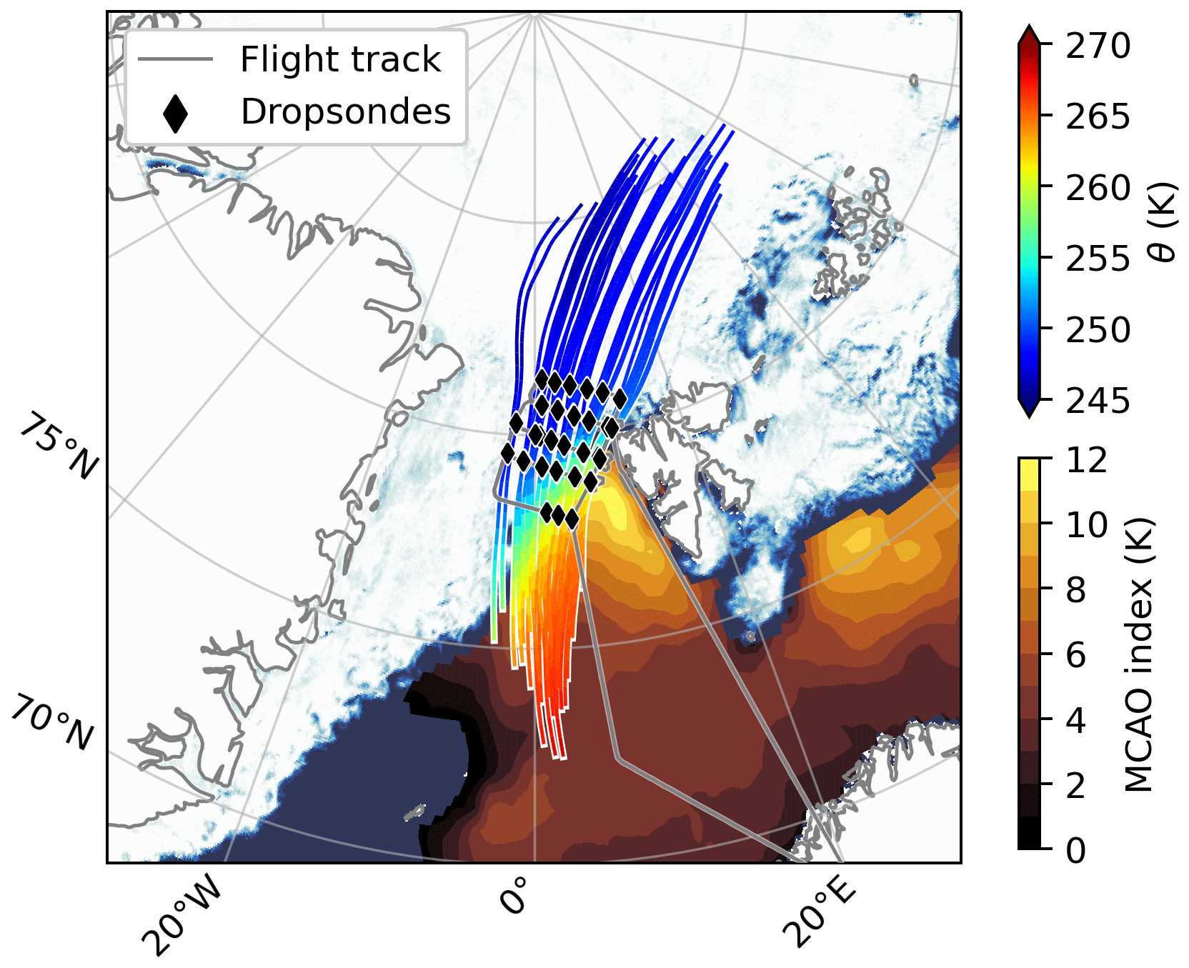
https://acp.copernicus.org/articles/24/3883/2024/acp-24-3883-2024-f01

Figure 1Case overview. The gray line shows the flight track of HALO on 1 April 2022. Diamond shapes show the locations where dropsondes were released. White-blueish contours represent 1 km high-resolution sea-ice concentration retrieved from a merged MODIS–AMSR2 satellite product (Ludwig et al., 2020). Over the ice-free ocean, yellow-brownish contours indicate the ERA5-derived CAO index M_850 hPa; see Eq. (3). Finally, the colored lines show 24 h backwards and 24 h forward trajectories initialized at the location of each dropsonde at 10 hPa above ground. The colors represent the evolving potential temperature (θ) of these air masses as traced from ERA5 data.

We analyze a set of 40 dropsondes which were released from HALO northwest of Svalbard. These RD94 dropsondes recorded air pressure p (accuracy 0.4 hPa), air temperature T (0.2 K), relative humidity RH (2 %), derived potential temperature θ, and specific humidity q, as well as horizontal wind components (0.2 m s⁻¹; Vaisala, 2010; George et al., 2021). The data were assimilated by the ECMWF Integrated Forecasting System (IFS), also serving as input for the ERA5 and CARRA reanalyses. The profiles of θ are used to derive the atmospheric BLH from dropsonde measurements and reanalyses. The BLH is defined here as the altitude where the largest vertical gradient in θ is found (similar to Seidel et al., 2010; Dai et al., 2014; Bakas et al., 2020; Sinclair et al., 2022). For estimating the cloud top heights (CTHs), the 532 nm backscatter ratio from the water vapor differential absorption (WALES) lidar is used (Wirth et al., 2009). WALES has a vertical resolution of 15 m. We define the CTH as the maximum altitude above ground where the backscatter ratio exceeds that of cloud-free sections. Cloud radar data from the HALO Microwave Package (HAMP) are used to additionally evaluate cloud evolution (Mech et al., 2014). The radar data have a vertical resolution of 30 m. Furthermore, to better understand the heating and moistening rates, airborne observations from HALO are used to estimate the surface sensible and latent heat fluxes (SSHF, SLHF), similar to Li et al. (2022). SSHF and SLHF are calculated based on the Coupled Ocean–Atmosphere Response Experiment (COARE) bulk air–sea flux algorithms and aerodynamic formulas (Fairall et al., 2003). COARE is widely used for the calculation of air–sea turbulent heat fluxes (Edson et al., 2013; Bharti et al., 2019; Lin et al., 2023) and has been found to perform the best among 12 examined bulk aerodynamic formulas (Brunke et al., 2003). The following basic equations were used to estimate SSHF and SLHF (Fairall et al., 2003):

\begin{matrix} (1) & SSHF = ρ_{air} C_{H} c_{p} | U_{10 m} | (T_{10 m} - T_{skin}), \\ (2) & SLHF = ρ_{air} C_{Q} L_{v} | U_{10 m} | (q_{10 m} - 0.98 q_{sat,skin}), \end{matrix}

where ρ_air denotes the air density (kg m⁻³), C_H and C_Q are the transfer coefficients for heat and humidity (dimensionless), c_p is the specific heat capacity at constant pressure (c_p=1004.7 $J {kg}^{- 1} K^{- 1}$ ), L_v is the latent heat of evaporation (L_v=2.5008 J kg⁻¹), U_10 m is the wind speed at 10 m height (m s⁻¹), (T_10 m−T_skin) is the temperature difference between the 10 m air temperature and skin temperature (K), and (q_10 m−0.98q_sat,skin) is the difference in specific humidity between the 10 m level and the specific saturation humidity taken at skin temperature ( kg kg⁻¹). The factor of 0.98 accounts for the reduction in vapor pressure resulting from a typical seawater salinity of 3.4 % (Fairall et al., 2003). Dropsonde profiles are used to extract ρ_air, U_10 m, T_10 m, and q_10 m via interpolation to the 10 m height level. The Video airbornE Longwave Observations within siX channels (VELOX) thermal infrared imager (Schäfer et al., 2022) is applied to obtain T_skin (accuracy 0.5 K) and q_sat,skin for the cloud-free sections. The transfer coefficients of heat and humidity are directly calculated using the most recent COARE 3.5 bulk air–sea algorithm (Edson et al., 2013; Bariteau et al., 2021). At winds speeds up to 20 m s⁻¹, COARE has a reported uncertainty of around 10 % (Fairall et al., 2003; Edson et al., 2013). Together with the measurement uncertainties, a combined uncertainty on the bulk fluxes (SSHF, SLHF) of at least 12 % is assumed. For the MIZ with its many open leads, the calculated fluxes were multiplied with the open sea fraction of a merged MODIS–AMSR2 satellite product (Ludwig et al., 2020). However, it should be stressed that the real surface heat fluxes can be assumed to be highly heterogeneous in the MIZ and thus prone to much higher uncertainties (Tetzlaff et al., 2015). Finally, to collect in situ cloud measurements, the Polar 6 aircraft sampled concurrently with HALO (Fig. S2). Polar 6 was based in Longyearbyen on Svalbard and was equipped with a wide range of in situ probes (Moser et al., 2023), including a Nevzorov sonde from which the liquid and frozen cloud water contents were obtained. For liquid water contents of around 0.05 g kg⁻¹ similar to that discussed here, the uncertainty on measurements is assumed to be at approximately 17 % of the observed values (Korolev et al., 1998; Lucke et al., 2022; Mech et al., 2022 a).

2.2 Reanalysis products

The ERA5 global reanalysis features a sophisticated four-dimensional variational data assimilation scheme and is based on ECMWF's IFS cycle 41r2 (Hersbach et al., 2020). ERA5 data fields have a temporal resolution of 1 h, have a horizontal grid resolution of 31 km, and are available on 137 model levels. The model levels start 10 m above ground level (m a.g.l.) and are then situated approximately every 20 m, with an increasing spacing upwards. Several studies note the high performance of ERA5 in the Arctic region (Graham et al., 2019 a; Wu et al., 2023), specifically in the Fram Strait region (Graham et al., 2019 b). Thus, numerous authors performing trajectory analysis in the Arctic rely on wind and meteorological data fields from ERA5 (e.g., Papritz and Spengler, 2017; Papritz, 2020; Dahlke et al., 2022; You et al., 2021 a; Kirbus et al., 2023 a, b; Svensson et al., 2023).

The CARRA regional reanalysis was specifically tailored towards the unique conditions in the Arctic environment, such as the prevailing cold surfaces on Arctic sea ice and ice sheets. Notably, it explicitly simulates a snow layer on sea ice. CARRA is based on the HARMONIE-AROME non-hydrostatic regional numerical weather prediction model, which is operational in the Nordic countries and several other European countries (Bengtsson et al., 2017; Yang et al., 2023). The reanalysis data can be retrieved for two distinct domains (CARRA-West covering Greenland and CARRA-East encompassing Svalbard and northern Scandinavia) that overlap in the vicinity of Svalbard (Yang et al., 2023). Boundary forcings are taken from ERA5. CARRA analysis fields have a temporal resolution of 3 h, a horizontal grid resolution of 2.5 km, and 65 vertical model levels. The model levels start 15 m a.g.l. and are then situated approximately every 30 m, with an increasing spacing upwards.

In this study, ERA5 and CARRA wind fields are used for trajectory calculations, thermodynamic profiles are extracted at the dropsonde locations, and several cloud-related parameters and turbulent energy fluxes are retrieved. Compared to ERA5, a larger amount of local observations is assimilated into CARRA's three-dimensional variational assimilation scheme, such as snow depths from satellite observations or actual measurements of glacier albedos. Satellite-borne sea-surface temperature and sea-ice data are assimilated at a higher spatial resolution compared to ERA5. Especially in areas with steep topography, the increased resolution of CARRA versus ERA5 is expected to better fit to observations (Yang et al., 2023). Isaksen et al. (2022) show that both reanalyses reproduce the key features of the observed exceptional warming over the Barents Sea. However, CARRA shows more spatial details and larger regional surface air temperature trends. Moore and Imrit (2022) investigate winds in the 40–100 km narrow Nares Strait northwest of Greenland. They find a significant underestimation of local wind speeds in ERA5, which on average reach 40 % of the observed values versus 80 % in CARRA. Box et al. (2023) evaluate five contemporary numerical prediction systems against in situ rainfall data from Greenland stations. CARRA shows the lowest average bias and the highest explained variance. Køltzow et al. (2022) systematically evaluate the representation of 10 m wind speed and 2 m air temperature against observations for the two CARRA domains. The largest differences between CARRA and ERA5 are found in regions with complex terrain and coastlines, as well as over the Arctic sea ice for 2 m air temperature in winter. Over flat terrain, the added value is especially obvious for the air temperature. With these reported advantages in mind, CARRA focuses solely on the European Arctic sector and starts only in 1991. The 3-hourly analysis fields must be combined with short-range forecasts to match the same 1-hourly resolution of ERA5 (Yang et al., 2023).

To classify the strength of the observed CAO, the marine cold-air-outbreak index M (Kolstad et al., 2009; Fletcher et al., 2016 b) is calculated based on ERA5 data and an 850 hPa reference level (Papritz et al., 2015; Papritz and Spengler, 2017; Knudsen et al., 2018; Dahlke et al., 2022; Geerts et al., 2022; Mateling et al., 2023). Using the potential temperature θ, M_850 hPa is computed as follows:

\begin{matrix} (3) & M_{850 hPa} = θ_{skin,ocean} - θ_{850 hPa}, \end{matrix}

where θ_skin,ocean denotes the potential skin temperature over ice-free ocean. A positive M_850 hPa over a large area indicates the presence of a CAO event. The daily M_850 hPa is averaged temporally from the hourly input data and spatially over a box surrounding Fram Strait. With an extent of 75–80° N and 10° W–10° E, this box is identical with previous studies (Papritz and Spengler, 2017; Dahlke et al., 2022). Consistent with the aforementioned works, CAO events can be classified as weak (M_850 hPa below 4 K), moderate (M_850 hPa between 4–8 K), or strong (M_850 hPa above 8 K).

2.3 Trajectory analysis

To evaluate whether the quasi-Lagrangian flight strategy on 1 April 2022 had been a success, both the ERA5 and CARRA three-dimensional wind fields are retrieved on model levels. Note that all 40 released dropsondes were assimilated by ECMWF, which greatly improves the reliability of trajectory calculations. As will be shown, no significant differences in calculated trajectories are found when using ERA5 or CARRA data. A comparison of the very similar wind profiles is given in Figs. S3 and S4. Køltzow et al. (2022) also reported only small differences between ERA5 and CARRA wind fields in areas with flat terrain, such as over the Arctic Ocean.

The Lagrangian Analysis Tool (LAGRANTO; Sprenger and Wernli, 2015) is then used to identify quasi-Lagrangian matches, where the same air masses were sampled within a 20 km radius below HALO twice, first at times t₁ and then again at t₂. Air masses are initialized every 1 min along HALO's flight track, vertically every 5 hPa between 250 hPa and the surface, and horizontally evenly spaced every 7 km in a 20 km radius. In total, 2.1 million trajectories are calculated 6 h forward in time. Caused by the vertical shear of wind direction and wind speed, the sampled air masses start moving in different directions. Only for a certain fraction, due to successful flight planning and/or some luck, are some of the same air masses sampled again in a different location and for a second time. A match is registered if the same air mass is seen again in the column below HALO within the same 20 km radius. In the final step, observations from dropsondes are included. Only those matches in the lowest 2 km are kept where the time difference between the matching air mass below the aircraft and the dropsonde in its time during descent is below 90 s. At a flight speed of around 800 km h⁻¹, this again corresponds to a maximum distance of 20 km. More details on the quasi-Lagrangian flight strategy during HALO-(AC)³ can be found in Wendisch et al. (2024). As matches are altitude-dependent, from the closest dropsonde the vertically nearest potential air temperature and specific humidity measurements are retained. Potential temperature is chosen instead of regular air temperature to focus on diabatic processes (Papritz and Spengler, 2017; Dahlke et al., 2022). Applying all filters yields approx. 24 200 quasi-Lagrangian matches. The net diabatic heating and moistening rates are calculated as

\begin{matrix} (4) & {(\frac{Δ θ}{Δ t})}_{net} = \frac{θ_{2} - θ_{1}}{t_{2} - t_{1}}, \end{matrix}

\begin{matrix} (5) & {(\frac{Δ q}{Δ t})}_{net} = \frac{q_{2} - q_{1}}{t_{2} - t_{1}} . \end{matrix}

The air mass transformations occurring in CAOs are primarily forced by the transition from closed sea ice to ice-free ocean (Pithan et al., 2018; Wendisch et al., 2023). Therefore, the quasi-Lagrangian matches are grouped by the time each air mass has spent over ice-free ocean. For all dropsonde locations, 12 h backward trajectories are calculated using ERA5 and for the air masses in the lowest 10 hPa (approx. 100 m) above ground. The sea-ice concentration (SIC) is traced along each trajectory (Fig. S1 in the Supplement). For this purpose, the merged MODIS and ASI-AMSR2 data at 1 km grid resolution generated by the University of Bremen (Ludwig et al., 2020) are interpolated to a 0.05°×0.05° latitude–longitude grid. The duration over ocean is defined as the time the air mass spends over ice-free ocean (sea-ice concentration SIC≤20 %) until it first reaches a SIC>20 %.

While the flight leg of Polar 6 on 1 April 2022 was aligned in parallel with HALO's center leg, it still covered different regions at different times than HALO, not least due to the much lower speed of Polar 6 of around 300 km h⁻¹. To make data comparable, the same approach is taken as for HALO: every 1 min along the flight track, air masses are initialized. However, due to the in situ sampling method, the air masses are started at the actual flight level of Polar 6 and SIC traced (Fig. S2). As a result, the in situ observations are transformed into the same coordinate system of time over ice-free ocean as for HALO, which is the assumed primary driver of the observed air mass transformations. Due to its limited range, Polar 6 only sampled the first 3 h of the CAO.

3 Results and discussion

3.1 Case overview

Figure 1 gives an overview of the conditions on 1 April 2022. The flight track of HALO and the dense grid of dropsondes released west of Svalbard are depicted. The daily averaged CAO index M_850 hPa in the Fram Strait box is found to be 7.7 K. This qualifies the CAO investigated here between a moderate and strong case, following the classification of Papritz and Spengler (2017) and Dahlke et al. (2022). According to the ERA5-based CAO climatology 1979–2020 by Dahlke et al. (2022), the median daily frequency of occurrence for CAOs in the Fram Strait is at around 50 %–70 % both in March and April. Furthermore, events of similar magnitude can be expected at around 40 % of all days (Dahlke et al., 2022). This means that on 1 April 2022, HALO sampled a quite typical event for this region and time of the year. Figure 1 also reveals a maximum M_850 hPa of above 12 K close to the marginal sea-ice zone. This highlights the strong temperature contrasts that the cool Arctic air masses experience when departing the closed Arctic sea ice.

To better comprehend the air mass flow, a set of 40 trajectories is initialized at the location of each dropsonde with 1 min temporal resolution. These trajectories are started at 10 hPa above ground and calculated both forwards and backwards in time over a 24 h period. The ERA5-derived potential temperature is then traced. As seen in Fig. 1, during their drift over closed Arctic sea ice, the near-surface air parcels do not undergo any significant diabatic temperature changes. However, once they cross the MIZ and reach the ice-free ocean, the air masses undergo a rapid diabatic heating of up to 20 K within 24 h.

3.2 Eulerian comparison of observations and reanalyses

3.2.1 Sea-ice and cloud structures

Figure 2 depicts a first comparison between observations and the reanalyses. Figure 2a shows the Terra/MODIS corrected reflectance from NASA Worldview for 1 April 2022 (NASA Worldview, 2023). From the satellite imagery, it becomes clear that the Arctic sea ice northwest of Svalbard features many leads on different length scales. However, the MIZ is rather sharp, and the transition from closed sea ice to ice-free ocean water typically occurs within less than 1 km distance. Over the ice-free ocean, cloud streets due to roll convection are evident. The cloud streets form along the prevailing wind direction. Furthermore, a clear lee effect due to Svalbard's mountain ranges is seen to the west of the archipelago.

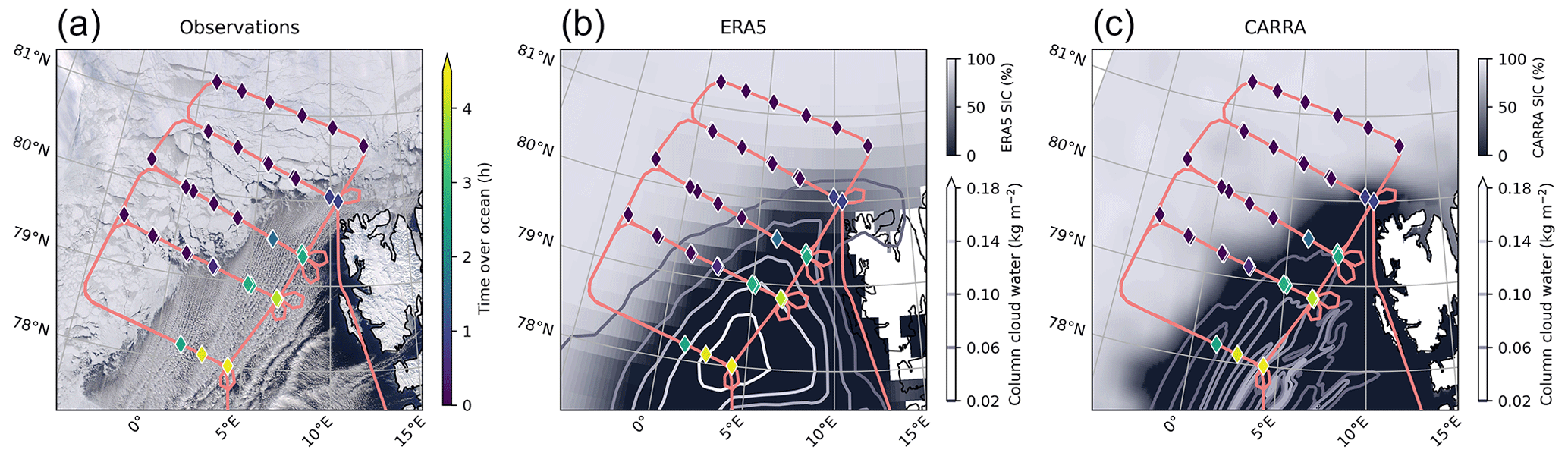
https://acp.copernicus.org/articles/24/3883/2024/acp-24-3883-2024-f02

Figure 2Sea-ice and cloud structures to the northwest of Svalbard on 1 April 2022 based on observations and reanalyses. In each subplot, the red line shows the flight path of HALO, and diamond shapes show the locations of released dropsondes. The shapes are colored by time near-surface air masses spent over ice-free ocean (sea-ice concentration SIC below 20 %; Ludwig et al., 2020). (a) The Terra/MODIS corrected reflectance shows the formation of cloud streets shortly after the off-ice drift. The image is taken from NASA Worldview (2023). (b) ERA5 data at 12:00 UTC. The SIC (filled contours) and the total column cloud liquid and ice water (contour lines) are shown. (c) CARRA data at 12:00 UTC. SIC (filled contours) and the total combined column cloud liquid, ice, and graupel water (contour lines) are depicted.

Figure 2b shows the corresponding fields as represented by ERA5 at 12:00 UTC noon. Due to its coarse spatial resolution, no leads are modeled in the SIC data fields, and the MIZ width is on a length scale of approximately 80 km. This is a typical MIZ width for ERA5 (Renfrew et al., 2021). Instead of cloud streets, a stratiform liquid and ice containing cloud deck is simulated, which thickens in off-ice direction. Clouds are partly also already formed over closed sea ice. In contrast, clouds in CARRA are exclusively formed over the ice-free ocean; see Fig. 2c. The high spatial resolution allows convection to be modeled. As a result, several distinct cloud streets are reproduced. In addition, CARRA better reproduces the sharp MIZ, which here is on the scale of around 10 km. The sharper MIZ of CARRA in comparison to ERA5 is not only a matter of spatial resolution (2.5 km for CARRA versus 30 km for ERA5). The sea-ice concentrations in ERA5 are derived from the Operational Sea Surface Temperature and Ice Analysis dataset, produced by the UK Met Office (OSTIA; Donlon et al., 2012). OSTIA outputs daily sea-surface temperature and sea-ice concentration fields based on satellite observations, with a native resolution of 0.05°×0.05° (roughly 6 km). Yet the sea-ice data are based on the EUMETSAT OSI-SAF 401 dataset utilizing 19 GHz and 37 GHz microwave channels at along-track resolutions of coarse 69 and 37 km (Tonboe et al., 2017; Renfrew et al., 2021). On the contrary, CARRA strongly relies on the European Space Agency's Sea Ice Climate Change Initiative product (SICCI; Toudal Pedersen et al., 2017) with a native resolution of 15–25 km. These data are additionally filtered based on the high-resolution sea-surface temperature fields and then regridded to the CARRA grid (Yang et al., 2023). Several authors noted that improved sea-ice and MIZ representation crucially improve the performance of models in the lower-tropospheric layers (Liu et al., 2006; Gryschka et al., 2008; Chechin et al., 2013; Müller et al., 2017; Spensberger and Spengler, 2021). As will be shown later, the magnitude of turbulent heat fluxes is directly correlated to the distribution of sea-ice versus ice-free ocean, which is the primary driver of CAO transformations. Errors in MIZ width can have significant downstream effects over several hundreds of kilometers (Tomassini et al., 2017; Spensberger and Spengler, 2021).

3.2.2 Vertical thermodynamic profiles

Figure 3a shows the profiles of air temperature from observations. Over sea ice, clear temperature inversions are found. The coldest near-surface temperatures reach −27 °C, and the thickness of the inversions is around 0.6–0.9 km. As air masses spend more time over ice-free waters, they become warmer near the surface, leading to stronger coupled ABLs and the development of a typical marine stratification. This is accompanied by a steady, linear increase in the calculated BLHs and closely correlated CTHs.

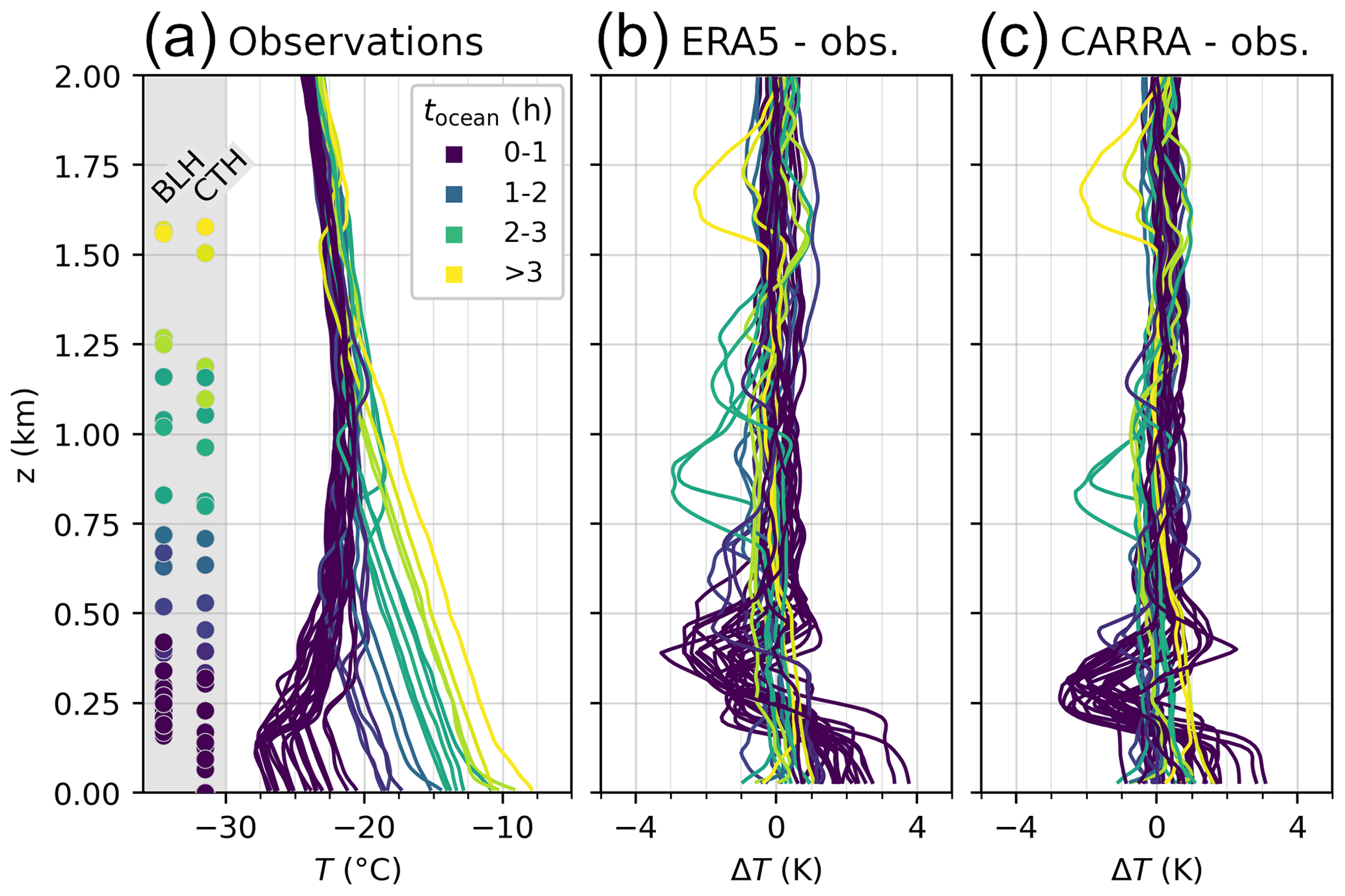
https://acp.copernicus.org/articles/24/3883/2024/acp-24-3883-2024-f03

Figure 3Vertical profiles of air temperature (T) in the lowest 2 km above ground taken from observations and reanalyses. In all panels, profiles are colored by the time air masses spent over open ocean. (a) Observed profiles of air temperature. Measurement-derived atmospheric BLHs and lidar-derived CTHs are indicated on the left-hand side. (b) Deviation of the ERA5 profiles from the observed profiles, and (c) deviation of the CARRA profiles from the observed profiles.

Download

By linearly interpolating all data to 100 m vertical resolution, the temperature differences ΔT between ERA5/CARRA and the observations are computed. The results are shown in Fig. 3b and c. Despite the reanalysis assimilating all the employed dropsondes, the ERA5 profiles show a distinct warm bias in near-surface air temperatures of mean 2 K over Arctic sea ice. Many authors reported on similar warm biases of skin and near-surface air temperatures in ERA5 (Batrak and Müller, 2019; Wang et al., 2019; Tjernström et al., 2021; McCusker et al., 2023). The skin temperatures are generally considered too warm as an insulating layer of snow is missing atop the floating ice, which can introduce surplus heat into the lower atmosphere (Batrak and Müller, 2019; Wang et al., 2019). The surface warm bias turns to a mean cold bias of −1 K at altitudes of 0.25–0.50 km. Over the ocean, the mean temperature bias is much lower and reaches −0.5 K at around 1 km altitude. In the CARRA data, the near-surface temperature bias is reduced to an average of 1 K. Similar improvements over ERA5 have been reported by others (Køltzow et al., 2022). However, CARRA also faces challenges in accurately representing temperature inversions. This is reflected in the cold bias of around −1.5 K at altitudes of 0.20–0.40 km.

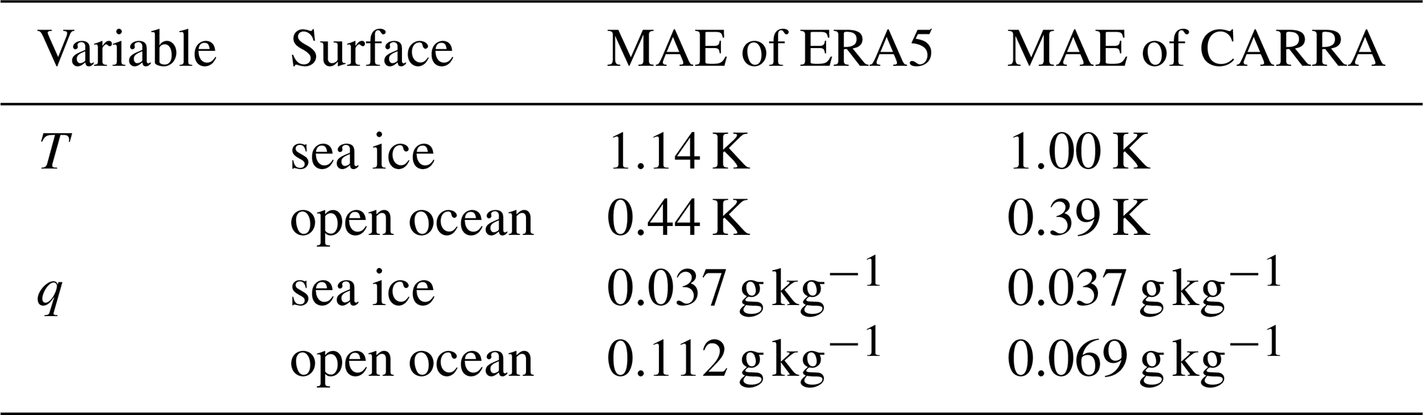
The mean absolute errors (MAEs) of ERA5 and CARRA with regards to measurements are computed. Output from both reanalyses as well as dropsondes is interpolated to a common vertical coordinate of altitude above ground in 10 m steps. To evaluate especially the crucial ABL representation, MAEs are averaged vertically from the surface up to the observation-derived BLHs, plus an additional 200 m margin to capture the dipole pattern of errors. Table 1 summarizes the results separately for dropsondes released over sea ice and ice-free ocean. For air temperature over ice, CARRA shows a slightly smaller MAE of 1.00 K versus 1.14 K for ERA5. Over the ice-free waters of Fram Strait, these errors are significantly reduced in both products, yielding a MAE of 0.39 K in CARRA and 0.44 K in ERA5.

Table 1Mean absolute errors (MAEs) of ERA5 and CARRA profiles compared to observations. The MAEs are averaged vertically up to the observed boundary-layer heights, plus an additional 200 m margin. Results are shown for the variables air temperature (T) and specific humidity (q), grouped by surface type. Profiles are classed as sea ice (open ocean) if the AMSR2 sea-ice concentrations is above (below) 50 %.

Download Print Version | Download XLSX

Next, the vertical profiles of specific humidity are examined. Figure 4a depicts the observed profiles, as extracted from the dropsonde measurements. Over sea ice, a uniform and dry ABL is found, where maximum values of around 0.6 g kg⁻¹ are measured. Near-surface layers are the driest, at around 0.4 g kg⁻¹. The longer the air masses reside over the sea, the more water vapor is picked up by the lower air mass layers through evaporation from the ocean surface.

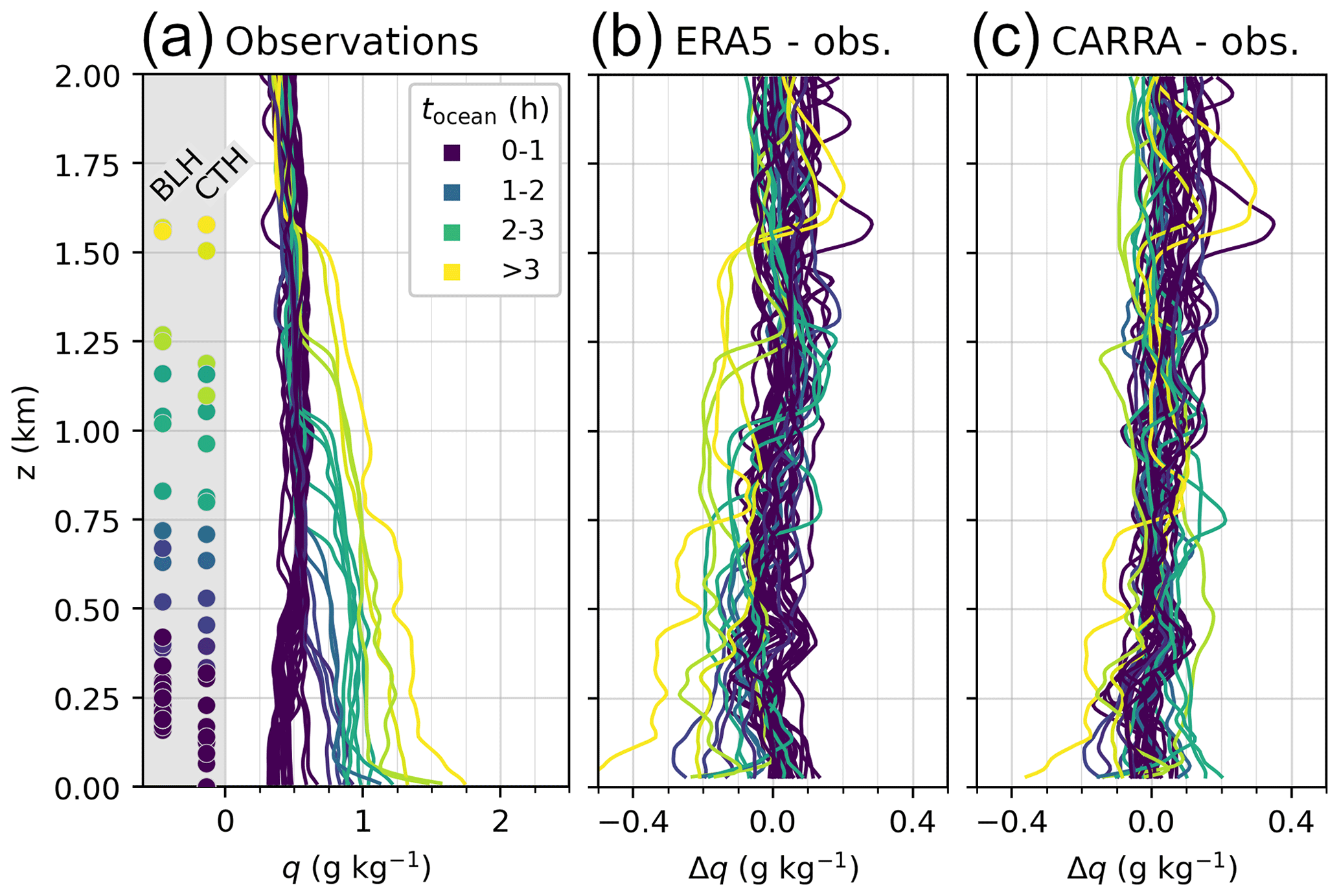
https://acp.copernicus.org/articles/24/3883/2024/acp-24-3883-2024-f04

Figure 4Same as Fig. 3 but for specific humidity in the lowest 2 km above ground. (a) Observed profiles of specific humidity. (b) Deviation of the ERA5 profiles from the observed profiles, and (c) deviation of the CARRA profiles from the observed profiles.

Download

Over sea ice, ERA5 shows a mean near-surface moist bias of 0.05 g kg⁻¹ (Fig. 4b), as well as a slight dry bias close to the BLHs. Once air masses drift over the sea, a strong dry bias is found throughout the ABL. It increases over time and reaches down to −0.5 g kg⁻¹, which corresponds to about 30 % of the observed values. CARRA shows different patterns (Fig. 4c). Over the closed ice pack, the lowest 0.2 km shows a negligible humidity bias. However, in higher layers above 0.5 km, a slight moist bias is seen. During the off-ice drift, at first a slight moist and later dry bias becomes obvious; however, this is much smaller compared to the ERA5 reanalysis. The same patterns are found in the quantified MAEs within the ABLs; see again Table 1. Notably, over the ice-free ocean, CARRA's MAE of 0.069 g kg⁻¹ is significantly lower than ERA5's MAE of 0.112 g kg⁻¹.

3.3 Quasi-Lagrangian comparison of observations and reanalyses

3.3.1 Quasi-Lagrangian matches

Figure 5 gives an overview of the quasi-Lagrangian matches calculated with reference to the dropsondes. All matches are colored by the time air masses spent over ice-free ocean. As described in the Methods (Sect. 2), these approximately 24 200 matches are a function of height above ground because not only are the zonal and meridional winds height-dependent, but also the vertical velocity is used for the three-dimensional trajectory calculations. This allows air masses to ascend or descend along their horizontal flow. The matches cover 150 km along the prevailing wind direction over the Arctic sea ice and about 200 km along the CAO evolution over ice-free ocean.

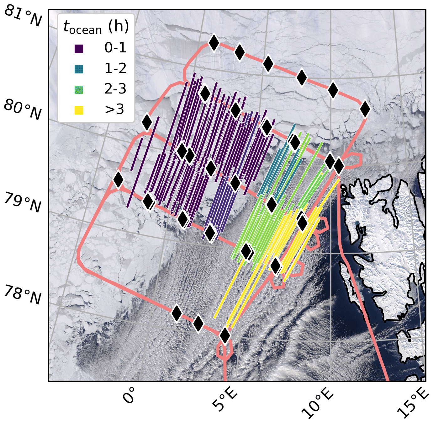
https://acp.copernicus.org/articles/24/3883/2024/acp-24-3883-2024-f05

Figure 5Spatial overview of the location of matching ERA5 trajectories, which were calculated with respect to a 20 km circle around the dropsondes. Matching lines are colored by the time air masses spent over ocean. The background Terra/MODIS satellite image is taken from NASA Worldview (2023).

Naturally, the question arises of how reliable the trajectory calculations presented here are. In previous studies, sometimes additional criteria were applied to prove the reliability of trajectories. These are similar hydrocarbon fingerprints between matches (Methven et al., 2006) or an inert perfluoromethylcyclopentane tracer being deployed (Boettcher et al., 2021). However, such a use of tracers is only possible in case of in situ sampling. In the CAO presented here, the assimilation of the high-density grid of dropsondes serves as crucial input for ERA5 and CARRA. This can also be seen in the comparison of wind profiles as shown in Figs. S3 and S4. With the exception of the nearest-surface layers, a close match is seen between dropsondes and both reanalyses. Also, as trajectories are only calculated over short spatiotemporal scales (on the order of 1–4 h, 50–200 km), small errors can not add up as much. For some research questions, it might be more valuable to investigate transformations over larger spatiotemporal scales, such as was done, for example, for aerosol and hydrocarbon species (Methven et al., 2006; Sanchez et al., 2022). However, as will be demonstrated, the highly important thermodynamic evolution occurs on timescales of a few hours and below. If too much time passes between two matching observations, the “net” rates, e.g. of $(Δ θ / Δ t)_{net}$ and $(Δ q / Δ t)_{net}$ introduced in Eqs. (4) and (5), would smooth out short-lived effects even more; models would be increasingly needed to disentangle the net rates calculated over longer time frames into sections of more or less intense transformations. Finally, the approach presented here of initializing and then registering matches for a large number of trajectories within a radius of 20 km around HALO's location is also essential to better assess the statistical significance of matches. Notably, all deviations seen between the aforementioned observed and modeled wind profiles result in an error of less than this 20 km radius over 1–3 h of drift.

3.3.2 Diabatic heating and moistening rates

The evolution of thermodynamic properties in the form of heating and moistening rates is analyzed in a quasi-Lagrangian framework, grouped by time air masses spent over ice-free ocean.

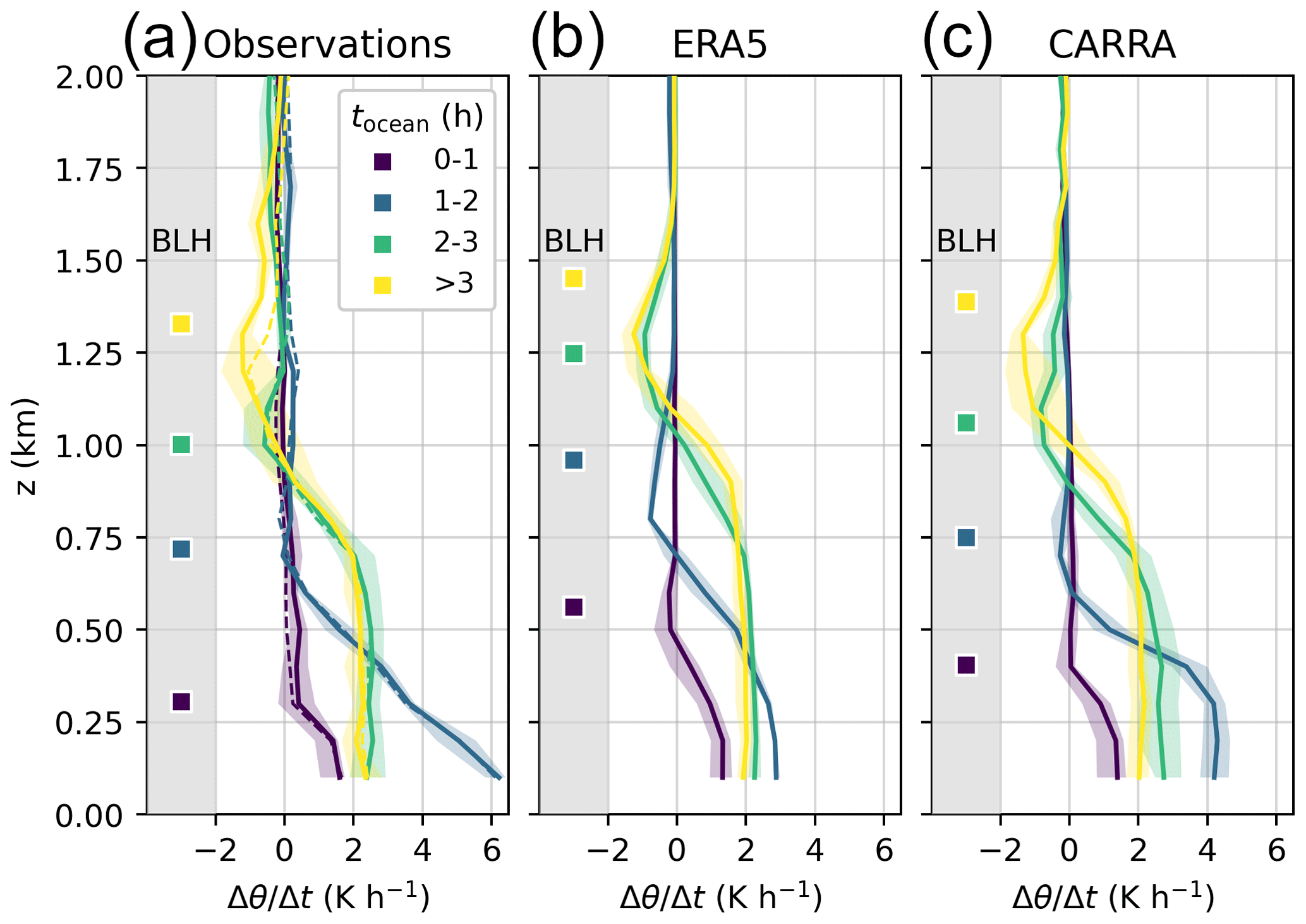
https://acp.copernicus.org/articles/24/3883/2024/acp-24-3883-2024-f06

Figure 6Diabatic heating rates grouped by time air masses spent over the ice-free ocean. On the left side of each panel, the mean BLH in each class is plotted as a square. Lines depict the mean values and shading the 25th–75th percentiles. (a) Heating rates based on the quasi-Lagrangian dropsonde observations. Solid lines are from ERA5 trajectories, and the dashes lines are from CARRA trajectories. (b) Corresponding heating rates extracted from ERA5. (c) Corresponding heating rates extracted from CARRA.

Download

First, the evolution of diabatic heating rates is analyzed. Figure 6a shows the vertically resolved diabatic heating rates based on the quasi-Lagrangian dropsonde observations. No significant differences exist between using ERA5 or CARRA winds as input. The MAE between ERA5 and CARRA heating rates in the lowest 1.5 km above ground and averaged for all times over ice-free ocean amounts to only 0.13 K h⁻¹. Note that air parcels of the first category (t_ocean=0–1 h) are drifting almost exclusively over sea ice and leads (Fig. 5). For these air masses, a maximum near-surface warming of around 1.8 K h⁻¹ is found. This possibly stems from some of the leads crossed by the trajectories. However, the heat is contained within the very shallow ABL, and all heating rates above the BLHs of around 0.30 km are around 0 K h⁻¹. After crossing the MIZ and reaching the ice-free ocean (t_ocean=1–2 h), a very intense surface warming is seen, where values larger than 6 K h⁻¹ are found. This heating is starting to be mixed upwards into the increasingly deep ABL, which reaches BLHs of around 0.70 km. After the initial rapid exposure of the cold and dry Arctic air masses to the much warmer ocean surface, the heating in the lowest layers declines rapidly and stays around 2 K h⁻¹. The vertical mixing is now dominating and leads to almost homogeneous mixing within the lowest 0.75 km of the troposphere. Interestingly, some layers above show regions with negative heating rates, i.e., a net cooling of air masses at altitudes around the BLHs. An analysis of ERA5 temperature tendencies indicates that this is not a sign of a net cloud-top radiative cooling effect but instead of the mixing of colder near-surface air with the original, overlying warmer air (Fig. S5). Previous airborne studies have shown that in the early stages of CAOs, the heat budget has several sources. Notably, the strong surface heat fluxes are reinforced by entrainment fluxes with the warmer inversion aloft. The relative contributions of the heat sources change with distance from the sea-ice edge. Over leads in the MIZ, entrainment heat fluxes exceeding 30 % of the surface heat fluxes have been observed in single cases (Tetzlaff et al., 2015). Shortly after passing the sea-ice edge, this ratio can initially increase to 80 %, which then again decreases to 30 % for fetches over 150 km (Brümmer, 1996). In the region of deep, cellular convection, condensation can even become the dominating contributor to air-mass heating (Brümmer, 1996). Overall, these previous studies indicate that the diabatic cooling near cloud tops corresponds to a warming below cloud tops, caused by the entrainment fluxes.

The ERA5-derived heating rates reflect the general features of the observations (Fig. 6b). This can be attributed to the assimilation of all 40 dropsondes into ERA5. However, some important differences are found. Over the Arctic sea ice, ERA5 shows BLHs almost twice as high as that seen in observations. While the slight surface warming of around 1.6–1.8 K h⁻¹ is also seen in ERA5, it shows excess heat that it mixes upwards towards the BLH. The intense surface warming at t_ocean=1–2 h is not represented in ERA5. This is in agreement with the sea-ice distribution shown on the overview map in Fig. 2b, which revealed a wide MIZ on the order of 80 km – much wider than that shown in the observations. As a result, the initial stage of the CAO is delayed in ERA5. The later stages (t_ocean>2 h) of the CAO, however, are represented rather well, yet again with an exaggerated vertical mixing. The essential feature of negative heating rates in higher altitudes is captured.

Figure 6c shows the heating rates extracted from the CARRA product. Generally, these settle in between the observations and ERA5. All BLHs are lower than in ERA5 and significantly closer to the observed values. For t_ocean=1–2 h, the observed intense warming rate higher than 6 K h⁻¹ is also not represented fully, yet it is much better than in ERA5. A maximum value for the near-surface heating of around 4 K h⁻¹ is found, which is homogeneously mixed upwards up to 0.40 km altitude. This might in part be caused by the much sharper MIZ, which is closer to reality (Fig. 2c).

In the early stage of CAOs, the primary source for turbulent heat fluxes is the warm ocean surface (Brümmer, 1996; Pithan et al., 2018). To study the evolution of the heating profiles along the CAO, it is thus essential to investigate the surface sensible heat fluxes (SSHFs). A comparison between the observation-derived and reanalysis-based SSHFs is given in Fig. 7a. All data are grouped by time spent over ice-free ocean. Over the Arctic sea ice and MIZ, the observation-derived SSHFs show a mean of below 50 W m⁻², with the 95th percentile peaking above 150 W m⁻². However, as was outlined in Sect. 2, the computation of turbulent heat fluxes over the sea ice and MIZ based on dropsondes is prone to high uncertainty. Both reanalyses show higher values, especially ERA5. For t_ocean=0–1 h, this corresponds to heating rates in both reanalyses being slightly too large and a mixing that is exaggerated.

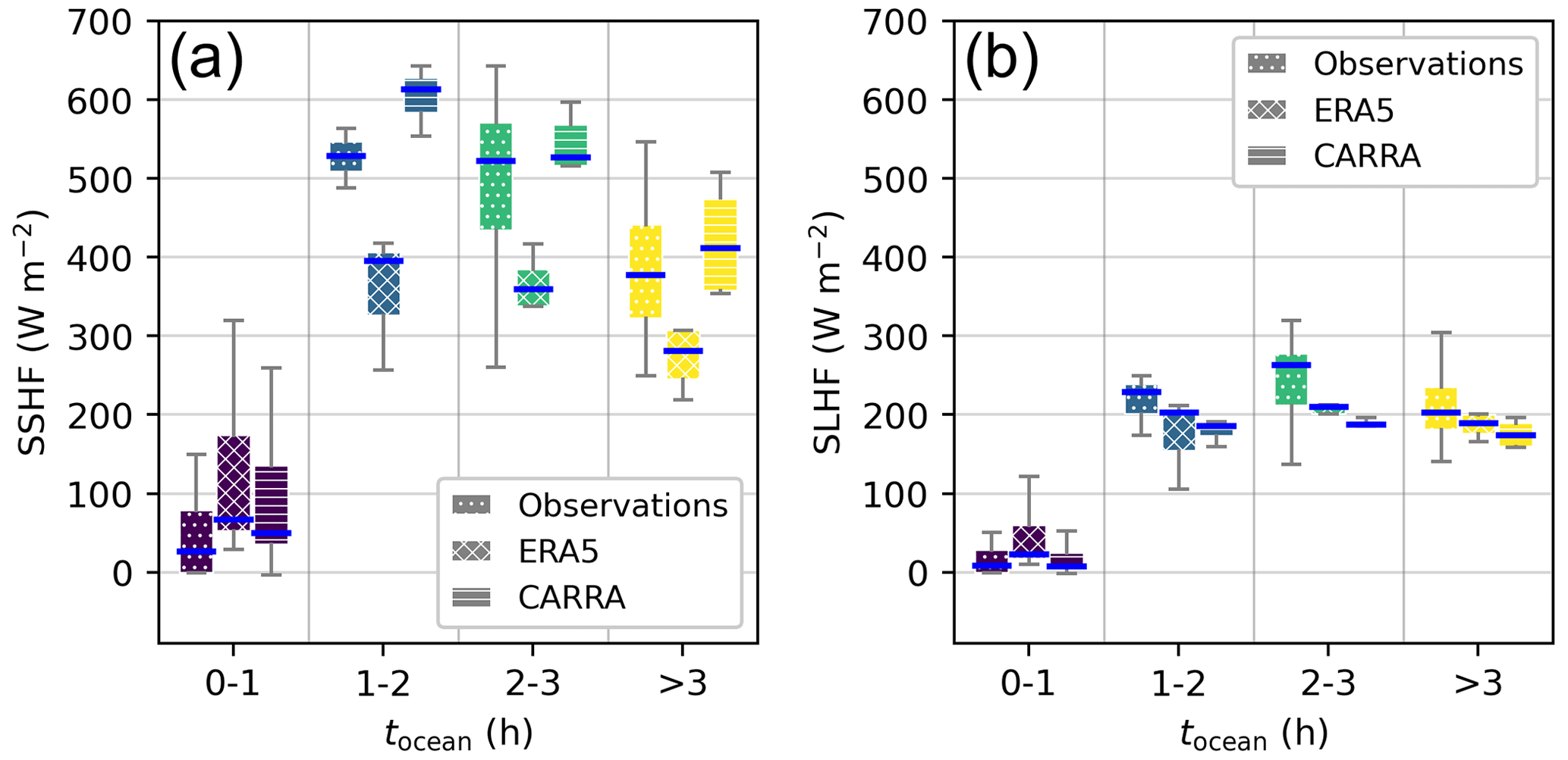
https://acp.copernicus.org/articles/24/3883/2024/acp-24-3883-2024-f07

Figure 7(a) Surface sensible heat fluxes (SSHFs) and (b) surface latent heat fluxes (SLHFs) as derived from observations, ERA5, and CARRA. Box plots show the median as thick lines, the 25th–75th percentiles as boxes, and the 5th–95th percentiles indicated as whiskers. Data are grouped by time over ice-free ocean.

Download

After the air masses cross the MIZ, large values of SSHF of around 520 W m⁻² are observed. Such values are typical in CAOs (Shapiro et al., 1987). ERA5 significantly underestimates the observed SSHFs by at least 130 W m⁻², while CARRA slightly exaggerates it. Later into the CAO, the observed SSHFs drop slightly yet are again best captured by CARRA. In general, the reduction of SSHFs over time is expected, as the temperature difference between the sea surface and the overlying air is reducing. This can potentially be counterbalanced, for example, by increasing underlying sea-surface temperatures, increased winds, or decreased surface roughness (Papritz and Spengler, 2017).

The different parameters that are required for the calculations of SSHF as shown in Eq. (1) are investigated in Fig. S6. Notably, over ocean both reanalyses significantly underestimate U_10 m, with CARRA being always closer to the observations. The horizontal thermal gradient between sea ice and the ice-free water surface causes a marked off-ice breeze, an analogue to sea–land breezes. Similar to that reported by Brümmer (1996), in our case, U_10 m reached its maximum near the sea-ice edge, and the off-ice acceleration due to thermal contrasts is estimated to be around 2.6 $m s^{- 1} h^{- 1}$ (calculations can be found in the Appendix). Therefore, the U_10 m in CARRA might be closer to observations than ERA5 as (i) the MIZ is narrower in CARRA and (ii) the discussed near-surface warm bias over sea ice is weaker in CARRA. Previous studies have also found ERA5 underestimates the highest near-surface winds over the ocean next to the MIZ, as well as SSHFs and SLHFs over the MIZ (Renfrew et al., 2021). Feeding coarse-resolution sea-ice data (with a MIZ of around 80 km, such as in ERA5) into higher-resolution models was also found to smear out the rapid increases in air temperature, wind speed, and surface fluxes (Renfrew et al., 2021).

In order to evaluate whether the differences between CARRA and ERA5 discovered for 1 April 2022 are of a systematic nature, a climatological comparison of SSHFs from both reanalyses for 1991–2022 can be found in Fig. S8. It shows that during CAO conditions, CARRA SSHFs are systematically larger than ERA5 SSHFs, and this is consistent over several decades. It is especially pronounced over ocean and corroborates our results for the case study of 1 April 2022. Similar systematic differences in the output surface turbulent heat fluxes have been reported also for comparisons of other reanalyses (Zhang et al., 2016; Taylor et al., 2018). Underestimated fluxes result in too-low uptake rates for heat and moisture, particularly close to the ice edge (Tomassini et al., 2017; Spensberger and Spengler, 2021). However, similar studies like Slättberg et al. (2023) are required for a deeper systematic evaluation of ERA5 versus CARRA, for example, to disentangle the combined effects on U_10 m as caused by MIZ width, parameterized surface roughness, or synoptic patterns.

Figure 8a shows the vertically resolved moistening rates based on the quasi-Lagrangian dropsonde observations. The MAE on the observed moisture uptake rates based on ERA5 versus CARRA trajectories as input is very low at 0.01 g kg⁻¹. For the air masses mostly sampled over sea ice, only minimal moisture uptake is found. The highest uptake at t_ocean=1–2 h reaches around 0.4 $g {kg}^{- 1} h^{- 1}$ at the surface. For longer times over the ice-free ocean, this moisture is then quickly mixed upwards. The magnitude of upward mixing partly exceeds the moisture uptake near the surface at later stages.

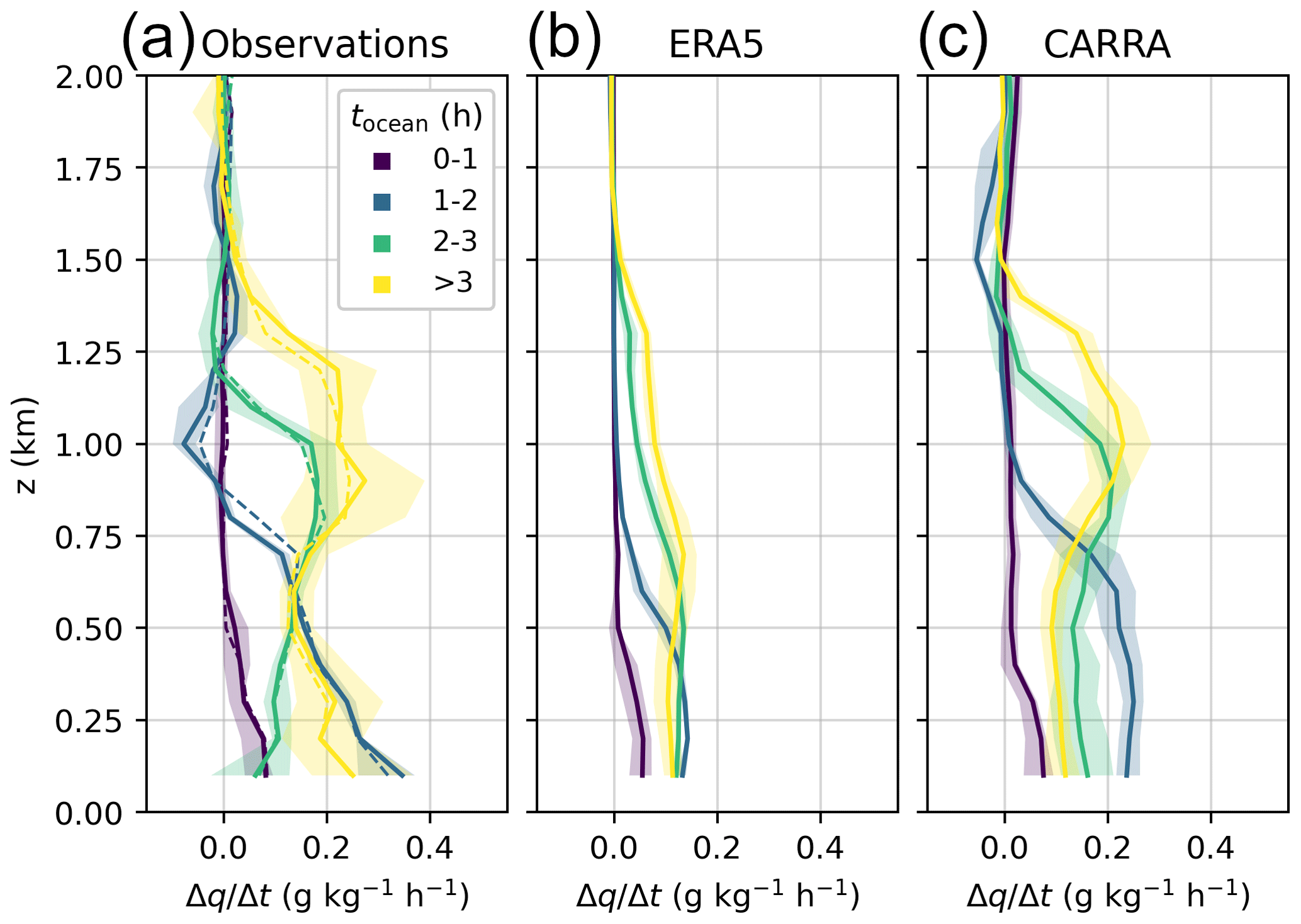
https://acp.copernicus.org/articles/24/3883/2024/acp-24-3883-2024-f08

Figure 8Moistening rates expressed as the change of specific humidity q per hour as a function of the time air masses spent over the ice-free ocean. Lines depict the mean values and shading the 25th–75th percentiles. (a) Moistening rates based on the quasi-Lagrangian dropsonde observations. Solid lines are from ERA5 trajectories, and the dashes lines are from CARRA trajectories. (b) Corresponding moistening rates extracted from ERA5. (c) Corresponding moistening rates extracted from CARRA.

Download

Figure 8b shows the corresponding rates as extracted from ERA5. ERA5 underestimates the near-surface moistening rates significantly; also layers further up show rates which are 2–3 times too low. CARRA performs better than ERA5 (Fig. 8c). Not only are the near-surface moistening rates closer to observations, but also the upward mixing is more realistic. An insufficient moistening rate within the lower troposphere during a CAO can be caused by (i) an insufficient supply of moisture from the surface, i.e., too-low SLHF, and/or (ii) an exaggerated removal of water vapor from the atmospheric column. Here, we check both factors separately.

Figure 7b compares the SLHFs between observations and the two reanalyses. Over sea ice, very low SLHFs with a median below 25 W m⁻² are found. Over the ocean, both ERA5 and CARRA underestimate the SLHF, and they are close to each other. Surprisingly, ERA5 always predicts slightly higher SLHFs than CARRA, which at first seems not to agree with the much lower moistening rates. Also the climatological comparison under CAO conditions shows that ERA5 SLHFs exhibit a constant bias towards larger values than in CARRA (Fig. S8). Overall, these findings hint towards mechanisms in ERA5 leading to an exaggerated removal of water vapor, namely cloud processes and precipitation. This is investigated in the next section.

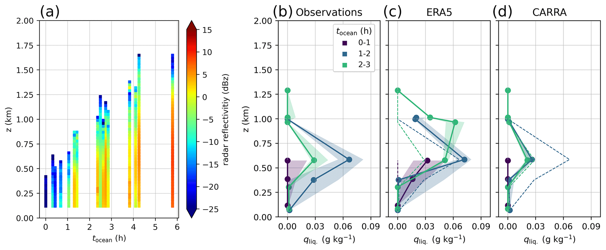
https://acp.copernicus.org/articles/24/3883/2024/acp-24-3883-2024-f09

Figure 9Vertical profiles of cloud structures, sorted by time air masses spent over ice-free ocean. (a) Profiles of the HAMP radar reflectivities measured aboard HALO. (b) Profiles of cloud liquid water content q_liq., based on a Nevzorov sonde aboard Polar 6, (c) q_liq. taken from ERA5, with the observed values as dashed lines, and (d) q_liq. taken from CARRA, with the observed values as dashed lines.

Download

3.3.3 Cloud properties

To help understand possible errors in the reanalyses connected to cloud physics, HAMP radar reflectivities from aboard HALO (Mech et al., 2014) as well as in situ Nevzorov measurements of cloud liquid water and ice contents by the Polar 6 aircraft are utilized (Lucke et al., 2022). A deeper investigation of cloud microphysical processes, such as riming, precipitation formation, or cloud street aspect ratios, is outside the scope of this article. However, details on these processes specifically including the CAO on 1 April 2022 are reported by Schirmacher et al. (2024) and Maherndl et al. (2023).

Figure 9a shows the measured HAMP radar reflectivity profiles averaged for 2 min around the time of each dropsonde release and up to 6 h into the CAO. The profiles are plotted as function of time air masses spent over ice-free ocean. For the locations over sea ice, either very low (radar reflectivity below −25 dBz) or no radar signals were recorded. As the air moves onto open waters, the radar reflectivities increase, and cloud tops are seen to rise linearly. Radar reflectivities for the first time cross the threshold of −5 dBz only for t_ocean>1 h. This indicates the presence of precipitation (Schirmacher et al., 2023; Maahn et al., 2014).

As Polar 6 has a range much lower than HALO, it was able to only sample the first 3 h of the CAO. Figure 9b–d shows the height-resolved measured specific cloud liquid water contents q_liq. Over the closed sea ice (Fig. 9b), in the sampled lowest 0.6 km above ground, no cloud liquid water was found, yet with low amounts at the top of the ABLs. After the drift across the MIZ, noticeable amounts of cloud water of up to 0.07 g kg⁻¹ are seen up to around 1 km altitude, which corresponds to the altitude of moisture uptake. Surprisingly, the liquid water content decreases in the next time step. This might be correlated with an increase of the frozen hydrometeors (i.e., cloud ice and snow) depicted in Fig. S7a. Several in situ probes confirm the occurrence of riming during the flight of Polar 6 (Maherndl et al., 2023). With the air temperatures always in the range of −25 to 0 °C (see Fig. 3), mixed-phase clouds are possible, and also the typical pattern of a supercooled layer above the ice layer is reproduced.

Figure 9c shows the cloud structures as reproduced by ERA5. ERA5 tends to overestimate the amount of liquid water present in the clouds. A similar enhanced abundance of liquid-bearing clouds especially over sea ice has been reported for the IFS, the model behind ERA5 (Tjernström et al., 2021; McCusker et al., 2023). In the CAO case here, this is in contrast to CARRA (Fig. 9d). With the exception of missing the strong increase in liquid clouds at t_ocean=1–2 h, CARRA matches the observations well. The overabundance of liquid-bearing clouds in ERA5 might explain the exaggerated vertical mixing of heat in ERA5. Even though ERA5 featured lower SSHFs compared to CARRA, the more pronounced cloud tops might lead to stronger entrainment fluxes. Also, the condensation into cloud droplets releases additional heat to the surrounding air masses.

Furthermore, total precipitation at the surface is much higher in ERA5 than in CARRA, which creates an additional sink for atmospheric moisture already over sea ice (Fig. 10). Precipitation over sea ice is unlikely based on the presented HAMP radar reflectivities. The −5 dBz threshold is only exceeded at t_ocean>1 h. This threshold translates to a precipitation rate of around 0.02–0.09 mm h⁻¹ (Maahn et al., 2014; Schirmacher et al., 2023). The statistical comparison between ERA5 and CARRA presented in Fig. S8 substantiates the finding of this case study. ERA5 has a strong bias to form liquid-bearing clouds already over sea ice and the MIZ. Over the ocean, there also is a strong bias towards higher cloud liquid hydrometeor contents. The ERA5 clouds systematically precipitate more strongly over the MIZ and ocean than clouds in CARRA. The significance of our findings is reinforced by McCusker et al. (2023), who showed that issues such as an overabundance of low, liquid-bearing clouds can propagate into higher-resolution models through large-scale forcings.

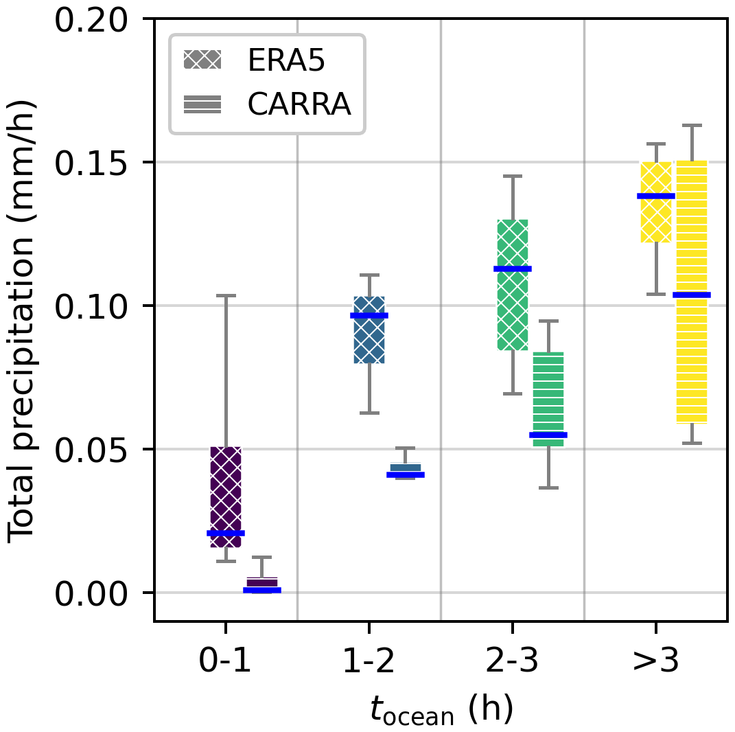
https://acp.copernicus.org/articles/24/3883/2024/acp-24-3883-2024-f10

Figure 10Total precipitation reaching surface level for ERA5 and CARRA. Box plots show the median as thick lines, the 25th–75th percentiles as boxes, and the 5th–95th percentiles as whiskers. Data are grouped by time over ice-free ocean.

Download

4 Summary and conclusions

We have presented a combined Eulerian and quasi-Lagrangian analysis of an Arctic marine cold-air outbreak (CAO). The CAO was closely sampled as part of the HALO-(AC)³ airborne campaign on 1 April 2022 in the Fram Strait, west of Svalbard. It was a representative CAO, which can be considered typical for this location and time of year as well as in its intensity. The performance of two state-of-the-art atmospheric reanalyses, ERA5 and CARRA, was evaluated against the measurements, with a focus on thermodynamic (air temperature, humidity) and cloud (cloud liquid water content) properties. We furthermore apply the quasi-Lagrangian approach to convert observations from both HALO and Polar 6 into a common coordinate system (time over ocean). The spatiotemporally highly resolved airborne measurements allow for a thorough characterization of the state of the lower troposphere over Arctic sea ice, the marginal sea-ice zone (MIZ), and the ice-free ocean. To the best of our knowledge, this is the first report on height-resolved diabatic heating and moistening rates in a developing CAO directly derived from quasi-Lagrangian observations. Going back to the research questions posed at the beginning of this article, we can answer them as follows.

Q1.
How do air temperature, specific humidity, and clouds evolve in the first 4 h of the developing CAO? Still over sea ice, some leads cause a weak heating and moisture uptake into the shallow atmospheric boundary layer of around 0.2 km height. Within the first hour of departing the closed sea ice, the strong contrast between the cold and dry Arctic air masses and the much warmer ocean causes a diabatic heating larger than 6 K h⁻¹ at the surface, a moisture uptake of more than 0.3 $g {kg}^{- 1} h^{- 1}$ , and the formation of mixed-phase clouds. As time progresses and clouds start forming, heat and moisture mix upwards vertically in the developing marine boundary layer. After 4 h, the atmospheric boundary-layer height exceeds 1.5 km. At around the boundary-layer heights, a slight net diabatic cooling and moisture loss are registered, which can be attributed to the upward mixing of air masses into the original, overlying warmer air.
Q2.
How do the ERA5 and CARRA reanalyses perform with respect to observations and compared to each other? In the Eulerian (i.e., fixed in space) framework, the coarse-resolution ERA5 reproduces some well-known issues. The skin and near-surface air temperatures are exaggerated, atmospheric boundary-layer heights are too large, and too many clouds are present. CARRA significantly improves all of these issues: for air temperature over sea ice, ERA5 features a mean absolute error (MAE) 14 % higher than CARRA (1.14 K versus 1.00 K), while for specific humidity over ice-free ocean the MAE is found to be 62 % higher in ERA5 compared to CARRA (0.112 g kg⁻¹ versus 0.069 g kg⁻¹). Taking the quasi-Lagrangian perspective, the heating rates are reasonably reproduced both in ERA5 and CARRA. However, the strong initial surface-based heating is not captured by ERA5. Even more pronounced are the differences in the moistening rates, where ERA5 estimates are up to 3 times too low and much better captured by CARRA. Overall, our height-resolved diabatic heating and moistening rates extend the quasi-Lagrangian, ERA5-based climatological CAO investigation of Papritz and Spengler (2017) to the vertical dimension. However, as the intense fluxes and transformations in the MIZ are not represented well by ERA5, the heating and especially moistening rates reported by them are likely biased towards lower values.
Q3.
What are some possible sources of errors which could explain deviations between reanalysis output and observations? Generally, uncertainties in reanalyses can stem from insufficient spatiotemporal resolution, different measurement sets being assimilated, and also the underlying model physics. The observed discrepancies between the two reanalyses and the observations result from the complex interplay of several processes. Over sea ice, the missing snow on ice layer leads to skin and near-surface air temperatures being too high in ERA5, which might explain the exaggerated boundary-layer heights. Moreover, it is well established that the MIZ is too wide in ERA5. Thus, turbulent fluxes are underestimated significantly in the first 2 to 3 h of the CAO. The reduced 10 m wind speeds might be related to the too-wide MIZ as well. Especially for the surface sensible heat flux, CARRA greatly improves on this. ERA5 forms liquid-bearing clouds too early and too thick. This can be due to too-warm initial temperatures or due to issues with the parameterization of the mixed-phase clouds, as well as a combination of both. In all stages investigated, ERA5 clouds thus precipitate considerably more than in CARRA, and too much water vapor is lost to this sink. A similar propagation of errors in initial conditions has been previously reported to affect the atmospheric state hundreds of kilometers downstream.

Overall, we find CARRA fulfilling its intended goal of improving on the global ERA5 reanalysis with regard to the thermodynamic and cloud evolution, based on the parameters investigated in the critical first 4 h of the CAO. CARRA might thus be better suited for driving higher-resolution models, such as large eddy simulations. While some climatological comparisons of differences between ERA5 and CARRA were supplied, deeper investigations are required to further support the statistical significance of our findings and to determine which components of CARRA are primarily responsible for the improvements. Ideally, these analyses should include extended data rows of observations, such as from regular radiosonde launches. Finally, the unprecedented quasi-Lagrangian observations collected during HALO-(AC)³ pose a rich database for future studies. For example, sensitivity studies could reveal the influence that initial aerosol concentrations (cloud-condensation nuclei, ice-nucleating particles) and different cloud schemes (one-moment or two-moment) have on the vertical mixing of heat and moisture, especially considering the intense surface forcings and additional entrainment fluxes.

Appendix A: Estimating the off-ice acceleration

One key parameter determining SSHF and SLHF is the 10 m wind speed U_10 m. As was already noted by Brümmer (1996), the horizontal thermal gradient between sea ice and the ice-free water surface causes a marked off-ice breeze, an analogue to sea–land breezes. In our case, U_10 m reached its maximum near the sea-ice edge, which has also been observed before by Brümmer (1996). The off-ice breeze can be estimated by starting with the static pressure equation:

\begin{matrix} (A1) & Δ p = - \frac{g p}{R T} Δ z, \end{matrix}

where Δp denotes the difference in pressure over a Δz deep ABL, g is the gravitational acceleration, p is the mean pressure, R is the gas constant for dry air, and T is the air temperature. By differentiating this equation with regard to T, we get

\begin{matrix} (A2) & d (Δ p) = \frac{g p}{R T^{2}} Δ z d T . \end{matrix}

In our case, a BLH of about 200 m thickness is found over sea ice. T shows an increase of 9 K over 100 km. A mean pressure of 1010 hPa and mean temperature of 255 K in the ABL are found. From this, a horizontal pressure gradient of around 1 hPa over 100 km results near the surface. While this appears small, the resulting pressure gradient force accelerates air masses in the off-ice direction:

\begin{matrix} (A3) & α = - \frac{1}{ρ} \frac{d p}{d x} . \end{matrix}

On 1 April 2022, this corresponds to an acceleration α of about 2.6 $m s^{- 1} h^{- 1}$ .

Data availability

Most airborne observational data used in this study were accessed through the ac3airborne module (https://doi.org/10.5281/zenodo.7305585, Mech et al., 2022 b), with the following exceptions. The Nevzorov liquid and total water contents are available from https://doi.org/10.1594/PANGAEA.963628 (Lucke et al., 2024). VELOX-derived skin temperature measurements can be obtained from https://doi.org/10.1594/PANGAEA.963401 (Schäfer et al., 2023). A Python implementation of the COARE 3.5 bulk air–sea flux algorithm is available from https://doi.org/10.5281/zenodo.5110991 (Bariteau et al., 2021). For CARRA, data are available on model levels (https://doi.org/10.24381/cds.d29ad2c6, Schyberg et al., 2020 a), pressure levels (https://doi.org/10.24381/cds.e3c841ad, Schyberg et al., 2020 b), and single levels (https://doi.org/10.24381/cds.713858f6, Schyberg et al., 2020 c). Further information can be found in CARRA's documentation (Yang et al., 2023) and user guide (Nielsen et al., 2023). ERA5 is also available on model levels (Hersbach et al., 2023 a), pressure levels (https://doi.org/10.24381/cds.bd0915c6, Hersbach et al., 2023 b), and single levels (https://doi.org/10.24381/cds.adbb2d47, Hersbach et al., 2023 c); see Hersbach et al. (2020).

Supplement

The supplement related to this article is available online at: https://doi.org/10.5194/acp-24-3883-2024-supplement.

Author contributions

BK, IS, MK, AE, and MW contributed to conception and design of the study. BK elaborated the methods, performed the analyses, created the figures, and prepared the original draft. IS and MK supported the development of analysis methods. MS provided the VELOX-derived skin temperature measurements. NS supported the processing and analysis of CARRA data. MM and JL provided and discussed the Nevzorov data. HM supported the processing of ERA5 data. All authors discussed the results, contributed to manuscript revision and approved the final submitted version.

Competing interests

The contact author has declared that none of the authors has any competing interests.

Disclaimer

Publisher's note: Copernicus Publications remains neutral with regard to jurisdictional claims made in the text, published maps, institutional affiliations, or any other geographical representation in this paper. While Copernicus Publications makes every effort to include appropriate place names, the final responsibility lies with the authors.

The results presented here contain modified C3S information. Neither the European Commission nor ECMWF is responsible for any use that may be made of the Copernicus information or data it contains.

Special issue statement

This article is part of the special issue “HALO-(AC)³ – an airborne campaign to study air mass transformations during warm-air intrusions and cold-air outbreaks”. It is not associated with a conference.

Acknowledgements

We gratefully acknowledge the funding and support of TRR 172 by the Deutsche Forschungsgemeinschaft (DFG, German Research Foundation), within the Transregional Collaborative Research Center's Arctic Amplification: Climate Relevant Atmospheric and Surface Processes, and Feedback Mechanisms (AC)³. We are furthermore grateful for funding and support by DFG within the framework of the priority program SPP 1294 to promote research with HALO. The publication of this article was supported by the Open Access Publication Funding program of the Publishing Fund of Leipzig University. We cordially thank the Alfred Wegener Institute, German Aerospace Center (DLR), as well as all aircraft crew and participants which made the HALO-(AC)³ campaign possible. We also thank the Institute of Environmental Physics at the University of Bremen for providing the merged MODIS–AMSR2 sea-ice concentration data (https://data.seaice.uni-bremen.de/modis_amsr2, last access: 20 October 2023). We acknowledge the use of imagery from the NASA Worldview application (https://worldview.earthdata.nasa.gov/, last access: 14 November 2023), part of the NASA Earth Observing System Data and Information System (EOSDIS).

Financial support

This research has been supported by the Deutsche Forschungsgemeinschaft (grants nos. 268020496 and 316646266).

Review statement

This paper was edited by Franziska Aemisegger and reviewed by two anonymous referees.

References

Bakas, N. A., Fotiadi, A., and Kariofillidi, S.: Climatology of the Boundary Layer Height and of the Wind Field over Greece, Atmosphere, 11, 910, https://doi.org/10.3390/atmos11090910, 2020. a

Bariteau, L., Blomquist, B., Fairall, C., Thompson, E., Jim, E., and Pincus, R.: Python implementation of the COARE 3.5 Bulk Air-Sea Flux algorithm, Zenodo [code], https://doi.org/10.5281/zenodo.5110991, 2021. a, b

Batrak, Y. and Müller, M.: On the warm bias in atmospheric reanalyses induced by the missing snow over Arctic sea-ice, Nat. Commun., 10, 4170, https://doi.org/10.1038/s41467-019-11975-3, 2019. a, b

Bengtsson, L., Andrae, U., Aspelien, T., Batrak, Y., Calvo, J., de Rooy, W., Gleeson, E., Hansen-Sass, B., Homleid, M., Hortal, M., Ivarsson, K.-I., Lenderink, G., Niemelä, S., Nielsen, K. P., Onvlee, J., Rontu, L., Samuelsson, P., Muñoz, D. S., Subias, A., Tijm, S., Toll, V., Yang, X., and Køltzow, M. Ø.: The HARMONIE–AROME model configuration in the ALADIN–HIRLAM NWP system, Mon. Weather Rev., 145, 1919–1935, 2017. a

Bharti, V., Schulz, E., Fairall, C. W., Blomquist, B. W., Huang, Y., Protat, A., Siems, S. T., and Manton, M. J.: Assessing Surface Heat Flux Products with In Situ Observations over the Australian Sector of the Southern Ocean, J. Atmos. Ocean. Tech., 36, 1849–1861, https://doi.org/10.1175/jtech-d-19-0009.1, 2019. a

Boettcher, M., Schäfler, A., Sprenger, M., Sodemann, H., Kaufmann, S., Voigt, C., Schlager, H., Summa, D., Di Girolamo, P., Nerini, D., Germann, U., and Wernli, H.: Lagrangian matches between observations from aircraft, lidar and radar in a warm conveyor belt crossing orography, Atmos. Chem. Phys., 21, 5477–5498, https://doi.org/10.5194/acp-21-5477-2021, 2021. a, b, c

Boucher, O., Randall, D., Artaxo, P., Bretherton, C., Feingold, G., Forster, P., Kerminen, V.-M., Kondo, Y., Liao, H., Lohmann, U., Rasch, P., Satheesh, S. K., Sherwood, S., Stevens, B., and Zhang, X. Y.: Clouds and Aerosols, in: Climate Change 2013 – The Physical Science Basis, Contribution of Working Group I to the Fifth Assessment Report of the Intergovernmental Panel on Climate Change, edited by: Stocker, T. F., Qin, D., Plattner, G.-K., Tignor, M., Allen, S. K., Doschung, J., Nauels, A., Xia, Y., Bex, V., and Midgley, P. M., Cambridge University Press, 571–658, https://doi.org/10.1017/cbo9781107415324.016, 2014. a

Box, J. E., Nielsen, K. P., Yang, X., Niwano, M., Wehrlé, A., van As, D., Fettweis, X., Køltzow, M. A. Ø., Palmason, B., Fausto, R. S., van den Broeke, M. R., Huai, B., Ahlstrøm, A. P., Langley, K., Dachauer, A., and Noël, B.: Greenland ice sheet rainfall climatology, extremes and atmospheric river rapids, Meteorol. Appl., 30, e2134 https://doi.org/10.1002/met.2134, 2023. a

Brümmer, B.: Boundary-layer modification in wintertime cold-air outbreaks from the Arctic sea ice, Bound.-Lay. Meteorol., 80, 109–125, https://doi.org/10.1007/bf00119014, 1996. a, b, c, d, e, f, g, h, i

Brümmer, B.: Roll and Cell Convection in Wintertime Arctic Cold-Air Outbreaks, J. Atmos. Sci., 56, 2613–2636, https://doi.org/10.1175/1520-0469(1999)056<2613:racciw>2.0.co;2, 1999. a

Brunke, M. A., Fairall, C. W., Zeng, X., Eymard, L., and Curry, J. A.: Which Bulk Aerodynamic Algorithms are Least Problematic in Computing Ocean Surface Turbulent Fluxes?, J. Climate, 16, 619–635, https://doi.org/10.1175/1520-0442(2003)016<0619:wbaaal>2.0.co;2, 2003. a

Businger, S., Johnson, R., and Talbot, R.: Scientific Insights from Four Generations of Lagrangian Smart Balloons in Atmospheric Research, B. Am. Meteorol. Soc., 87, 1539–1554, https://doi.org/10.1175/bams-87-11-1539, 2006. a

Chechin, D. G., Lüpkes, C., Repina, I. A., and Gryanik, V. M.: Idealized dry quasi 2-D mesoscale simulations of cold-air outbreaks over the marginal sea ice zone with fine and coarse resolution, J. Geophys. Res.-Atmos., 118, 8787–8813, https://doi.org/10.1002/jgrd.50679, 2013. a

Christensen, M. W., Jones, W. K., and Stier, P.: Aerosols enhance cloud lifetime and brightness along the stratus-to-cumulus transition, P. Natl. Acad. Sci. USA, 117, 17591–17598, https://doi.org/10.1073/pnas.1921231117, 2020. a

Dahlke, S., Solbès, A., and Maturilli, M.: Cold Air Outbreaks in Fram Strait: Climatology, Trends, and Observations During an Extreme Season in 2020, J. Geophys. Res.-Atmos., 127, e2021JD035741, https://doi.org/10.1029/2021JD035741, 2022. a, b, c, d, e, f, g, h, i, j, k, l, m, n, o, p

Dai, C., Wang, Q., Kalogiros, J. A., Lenschow, D. H., Gao, Z., and Zhou, M.: Determining Boundary-Layer Height from Aircraft Measurements, Bound.-Lay. Meteorol., 152, 277–302, https://doi.org/10.1007/s10546-014-9929-z, 2014. a

Donlon, C. J., Martin, M., Stark, J., Roberts-Jones, J., Fiedler, E., and Wimmer, W.: The Operational Sea Surface Temperature and Sea Ice Analysis (OSTIA) system, Remote Sens. Environ., 116, 140–158, https://doi.org/10.1016/j.rse.2010.10.017, 2012. a

Edson, J. B., Jampana, V., Weller, R. A., Bigorre, S. P., Plueddemann, A. J., Fairall, C. W., Miller, S. D., Mahrt, L., Vickers, D., and Hersbach, H.: On the Exchange of Momentum over the Open Ocean, J. Phys. Oceanogr., 43, 1589–1610, https://doi.org/10.1175/jpo-d-12-0173.1, 2013. a, b, c

Fairall, C. W., Bradley, E. F., Hare, J., Grachev, A. A., and Edson, J. B.: Bulk parameterization of air–sea fluxes: Updates and verification for the COARE algorithm, J. Climate, 16, 571–591, https://doi.org/10.1175/1520-0442(2003)016<0571:BPOASF>2.0.CO;2, 2003. a, b, c, d

Field, P. R., Brozz̆ková, R., Chen, M., Dudhia, J., Lac, C., Hara, T., Honnert, R., Olson, J., Siebesma, P., de Roode, S., Tomassini, L., Hill, A., and McTaggart-Cowan, R.: Exploring the convective grey zone with regional simulations of a cold air outbreak, Q. J. Roy. Meteor. Soc., 143, 2537–2555, https://doi.org/10.1002/qj.3105, 2017. a

Fletcher, J., Mason, S., and Jakob, C.: The Climatology, Meteorology, and Boundary Layer Structure of Marine Cold Air Outbreaks in Both Hemispheres, J. Climate, 29, 1999–2014, https://doi.org/10.1175/JCLI-D-15-0268.1, 2016a. a, b, c, d

Fletcher, J. K., Mason, S., and Jakob, C.: A climatology of clouds in marine cold air outbreaks in both hemispheres, J. Climate, 29, 6677–6692, 2016b. a

Geerts, B., Giangrande, S. E., McFarquhar, G. M., Xue, L., Abel, S. J., Comstock, J. M., Crewell, S., DeMott, P. J., Ebell, K., Field, P., Hill, T. C. J., Hunzinger, A., Jensen, M. P., Johnson, K. L., Juliano, T. W., Kollias, P., Kosovic, B., Lackner, C., Luke, E., Lüpkes, C., Matthews, A. A., Neggers, R., Ovchinnikov, M., Powers, H., Shupe, M. D., Spengler, T., Swanson, B. E., Tjernström, M., Theisen, A. K., Wales, N. A., Wang, Y., Wendisch, M., and Wu, P.: The COMBLE campaign: A study of marine boundary layer clouds in arctic cold-Air Outbreaks, B. Am. Meteorol. Soc., 103, E1371–E1389, https://doi.org/10.1175/BAMS-D-21-0044.1, 2022. a, b, c

George, G., Stevens, B., Bony, S., Pincus, R., Fairall, C., Schulz, H., Kölling, T., Kalen, Q. T., Klingebiel, M., Konow, H., Lundry, A., Prange, M., and Radtke, J.: JOANNE: Joint dropsonde Observations of the Atmosphere in tropical North atlaNtic meso-scale Environments, Earth Syst. Sci. Data, 13, 5253–5272, https://doi.org/10.5194/essd-13-5253-2021, 2021. a

Graham, R., Cohen, L., Ritzhaupt, N., Segger, B., Graversen, R., Rinke, A., Walden, V. P., Granskog, M. A., and Hudson, S. R.: Evaluation of six atmospheric reanalyses over Arctic sea ice from winter to early summer, J. Climate, 32, 4121–4143, https://doi.org/10.1175/JCLI-D-18-0643.1, 2019a. a

Graham, R. M., Hudson, S. R., and Maturilli, M.: Improved Performance of ERA5 in Arctic Gateway Relative to Four Global Atmospheric Reanalyses, Geophys. Res. Lett., 46, 6138–6147, https://doi.org/10.1029/2019GL082781, 2019b. a

Gryschka, M., Drüe, C., Etling, D., and Raasch, S.: On the influence of sea-ice inhomogeneities onto roll convection in cold-air outbreaks, Geophys. Res. Lett., 35, L23804, https://doi.org/10.1029/2008gl035845, 2008. a

Hersbach, H., Bell, B., Berrisford, P., Hirahara, S., Horányi, A., Muñoz-Sabater, J., Nicolas, J., Peubey, C., Radu, R., Schepers, D., Simmons, A., Soci, C., Abdalla, S., Abellan, X., Balsamo, G., Bechtold, P., Biavati, G., Bidlot, J., Bonavita, M., De Chiara, G., Dahlgren, P., Dee, D., Diamantakis, M., Dragani, R., Flemming, J., Forbes, R., Fuentes, M., Geer, A., Haimberger, L., Healy, S., Hogan, R. J., Hólm, E., Janisková, M., Keeley, S., Laloyaux, P., Lopez, P., Lupu, C., Radnoti, G., de Rosnay, P., Rozum, I., Vamborg, F., Villaume, S., and Thépaut, J.-N.: The ERA5 global reanalysis, Q. J. Roy. Meteor. Soc., 146, 1999–2049, https://doi.org/10.1002/qj.3803, 2020. a, b, c

Hersbach, H., Bell, B., Berrisford, P., Biavati, G., Horányi, A., Muñoz Sabater, J., Nicolas, J., Peubey, C., Radu, R., Rozum, I., Schepers, D., Simmons, A., Soci, C., Dee, D., and Thépaut, J.-N.: ERA5-hourly data on model levels, ECMWF [data set], http://apps.ecmwf.int/data-catalogues/era5 (last access: 5 November 2023), 2023a. a

Hersbach, H., Bell, B., Berrisford, P., Biavati, G., Horányi, A., Muñoz Sabater, J., Nicolas, J., Peubey, C., Radu, R., Rozum, I., Schepers, D., Simmons, A., Soci, C., Dee, D., and Thépaut, J.-N.: ERA5-hourly data on pressure levels from 1940 to present, Copernicus Climate Change Service (C3S) Climate Data Store (CDS) [data set], https://doi.org/10.24381/cds.bd0915c6, 2023b. a

Hersbach, H., Bell, B., Berrisford, P., Biavati, G., Horányi, A., Muñoz Sabater, J., Nicolas, J., Peubey, C., Radu, R., Rozum, I., Schepers, D., Simmons, A., Soci, C., Dee, D., and Thépaut, J.-N.: ERA5-hourly data on single levels from 1940 to present, Copernicus Climate Change Service (C3S) Climate Data Store (CDS) [data set], https://doi.org/10.24381/cds.adbb2d47, 2023c. a

Isaksen, K., Nordli, Ø., Ivanov, B., Køltzow, M. A. Ø., Aaboe, S., Gjelten, H. M., Mezghani, A., Eastwood, S., Førland, E., Benestad, R. E., Hanssen-Bauer, I., Brækkan, R., Sviashchennikov, P., Demin, V., Revina, A., and Karandasheva, T.: Exceptional warming over the Barents area, Sci. Rep.-UK, 12, 9371, https://doi.org/10.1038/s41598-022-13568-5, 2022. a

Kirbus, B., Chylik, J., Ehrlich, A., Becker, S., Schäfer, M., Neggers, R., and Wendisch, M.: Analysis of an Arctic cold air outbreak during autumn and related air mass transformations forced by surface changes and advection in higher altitudes, Elem. Sci. Anth., 11, 00079, https://doi.org/10.1525/elementa.2023.00079, 2023a. a

Kirbus, B., Tiedeck, S., Camplani, A., Chylik, J., Crewell, S., Dahlke, S., Ebell, K., Gorodetskaya, I., Griesche, H., Handorf, D., Höschel, I., Lauer, M., Neggers, R., Rückert, J., Shupe, M. D., Spreen, G., Walbröl, A., Wendisch, M., and Rinke, A.: Surface impacts and associated mechanisms of a moisture intrusion into the Arctic observed in mid-April 2020 during MOSAiC, Front. Earth Sci., 11, 1147848, https://doi.org/10.3389/feart.2023.1147848, 2023b. a

Knudsen, E. M., Heinold, B., Dahlke, S., Bozem, H., Crewell, S., Gorodetskaya, I. V., Heygster, G., Kunkel, D., Maturilli, M., Mech, M., Viceto, C., Rinke, A., Schmithüsen, H., Ehrlich, A., Macke, A., Lüpkes, C., and Wendisch, M.: Meteorological conditions during the ACLOUD/PASCAL field campaign near Svalbard in early summer 2017, Atmos. Chem. Phys., 18, 17995–18022, https://doi.org/10.5194/acp-18-17995-2018, 2018. a

Kolstad, E.: Higher ocean wind speeds during marine cold air outbreaks, Q. J. Roy. Meteorol. Soc., 143, 2084–2092, https://doi.org/10.1002/qj.3068, 2017. a

Kolstad, E. W. and Bracegirdle, T. J.: Marine cold-air outbreaks in the future: an assessment of IPCC AR4 model results for the Northern Hemisphere, Clim. Dynam., 30, 871–885, https://doi.org/10.1007/s00382-007-0331-0, 2007. a

Kolstad, E. W., Bracegirdle, T. J., and Seierstad, I. A.: Marine cold-air outbreaks in the North Atlantic: temporal distribution and associations with large-scale atmospheric circulation, Clim. Dynam., 33, 187–197, https://doi.org/10.1007/s00382-008-0431-5, 2009. a

Køltzow, M., Schyberg, H., Støylen, E., and Yang, X.: Value of the Copernicus Arctic Regional Reanalysis (CARRA) in representing near-surface temperature and wind speed in the north-east European Arctic, Polar Res., 41, 8002, https://doi.org/10.33265/polar.v41.8002, 2022. a, b, c

Korolev, A. V., Strapp, J. W., Isaac, G. A., and Nevzorov, A. N.: The Nevzorov Airborne Hot-Wire LWC–TWC Probe: Principle of Operation and Performance Characteristics, J. Atmos. Ocean. Tech., 15, 1495–1510, https://doi.org/10.1175/1520-0426(1998)015<1495:tnahwl>2.0.co;2, 1998. a

Krautstrunk, M. and Giez, A.: The Transition From FALCON to HALO Era Airborne Atmospheric Research, Springer Berlin Heidelberg, 609–624, https://doi.org/10.1007/978-3-642-30183-4_37, 2012. a

Landgren, O. A., Seierstad, I. A., and Iversen, T.: Projected future changes in Marine Cold-Air Outbreaks associated with Polar Lows in the Northern North-Atlantic Ocean, Clim. Dynam., 53, 2573–2585, 2019. a, b, c, d

Li, J., Yi, Y., Minnis, P., Huang, J., Yan, H., Ma, Y., Wang, W., and Kirk Ayers, J.: Radiative effect differences between multi-layered and single-layer clouds derived from CERES, CALIPSO, and CloudSat data, J. Quant. Spectrosc. Ra., 112, 361–375, https://doi.org/10.1016/j.jqsrt.2010.10.006, 2011. a

Li, X.-Y., Wang, H., Chen, J., Endo, S., George, G., Cairns, B., Chellappan, S., Zeng, X., Kirschler, S., Voigt, C., Sorooshian, A., Crosbie, E., Chen, G., Ferrare, R. A., Gustafson, W. I., Hair, J. W., Kleb, M. M., Liu, H., Moore, R., Painemal, D., Robinson, C., Scarino, A. J., Shook, M., Shingler, T. J., Thornhill, K. L., Tornow, F., Xiao, H., Ziemba, L. D., and Zuidema, P.: Large-Eddy Simulations of Marine Boundary Layer Clouds Associated with Cold-Air Outbreaks during the ACTIVATE Campaign. Part I: Case Setup and Sensitivities to Large-Scale Forcings, J. Atmos. Sci., 79, 73–100, https://doi.org/10.1175/jas-d-21-0123.1, 2022. a, b, c

Lin, J., Wang, Y., Pan, H., Wei, Z., and Xu, T.: Uncertainty of CYGNSS-Derived Heat Flux Variations at Diurnal to Seasonal Time Scales over the Tropical Oceans, Remote Sens.-Basel, 15, 3161, https://doi.org/10.3390/rs15123161, 2023. a

Linke, O., Quaas, J., Baumer, F., Becker, S., Chylik, J., Dahlke, S., Ehrlich, A., Handorf, D., Jacobi, C., Kalesse-Los, H., Lelli, L., Mehrdad, S., Neggers, R. A. J., Riebold, J., Saavedra Garfias, P., Schnierstein, N., Shupe, M. D., Smith, C., Spreen, G., Verneuil, B., Vinjamuri, K. S., Vountas, M., and Wendisch, M.: Constraints on simulated past Arctic amplification and lapse rate feedback from observations, Atmos. Chem. Phys., 23, 9963–9992, https://doi.org/10.5194/acp-23-9963-2023, 2023. a

Liu, A. Q., Moore, G. W. K., Tsuboki, K., and Renfrew, I. A.: The Effect of the Sea-ice Zone on the Development of Boundary-layer Roll Clouds During Cold Air Outbreaks, Bound.-Lay. Meteorol., 118, 557–581, https://doi.org/10.1007/s10546-005-6434-4, 2006. a

Lloyd, G., Choularton, T. W., Bower, K. N., Gallagher, M. W., Crosier, J., O'Shea, S., Abel, S. J., Fox, S., Cotton, R., and Boutle, I. A.: In situ measurements of cloud microphysical and aerosol properties during the break-up of stratocumulus cloud layers in cold air outbreaks over the North Atlantic, Atmos. Chem. Phys., 18, 17191–17206, https://doi.org/10.5194/acp-18-17191-2018, 2018. a

Lucke, J., Jurkat-Witschas, T., Heller, R., Hahn, V., Hamman, M., Breitfuss, W., Bora, V. R., Moser, M., and Voigt, C.: Icing wind tunnel measurements of supercooled large droplets using the 12 mm total water content cone of the Nevzorov probe, Atmos. Meas. Tech., 15, 7375–7394, https://doi.org/10.5194/amt-15-7375-2022, 2022. a, b

Lucke, J., Moser, M., De La Torre Castro, E., Mayer, J., and Voigt, C.: Nevzorov LWC and TWC data from the HALO-AC³ campaign in March and April 2022, PANGAEA [data set], https://doi.org/10.1594/PANGAEA.963628, 2024. a

Ludwig, V., Spreen, G., and Pedersen, L. T.: Evaluation of a new merged sea-ice concentration dataset at 1 km resolution from thermal infrared and passive microwave satellite data in the Arctic, Remote Sens.-Basel, 12, 3183, https://doi.org/10.3390/rs12193183, 2020. a, b, c, d

Maahn, M., Burgard, C., Crewell, S., Gorodetskaya, I. V., Kneifel, S., Lhermitte, S., Van Tricht, K., and van Lipzig, N. P. M.: How does the spaceborne radar blind zone affect derived surface snowfall statistics in polar regions?, J. Geophys. Res.-Atmos., 119, 13604–13620, https://doi.org/10.1002/2014JD022079, 2014. a, b

Maherndl, N., Moser, M., Lucke, J., Mech, M., Risse, N., Schirmacher, I., and Maahn, M.: Quantifying riming from airborne data during HALO-(AC)³, EGUsphere [preprint], https://doi.org/10.5194/egusphere-2023-1118, 2023. a, b

Mateling, M. E., Pettersen, C., Kulie, M. S., and L'Ecuyer, T. S.: Marine cold-air outbreak snowfall in the north Atlantic: A CloudSat perspective, J. Geophys. Res., 128, e2022JD038053, https://doi.org/10.1029/2022JD038053, 2023. a, b, c

McCusker, G. Y., Vüllers, J., Achtert, P., Field, P., Day, J. J., Forbes, R., Price, R., O'Connor, E., Tjernström, M., Prytherch, J., Neely III, R., and Brooks, I. M.: Evaluating Arctic clouds modelled with the Unified Model and Integrated Forecasting System, Atmos. Chem. Phys., 23, 4819–4847, https://doi.org/10.5194/acp-23-4819-2023, 2023. a, b, c

Mech, M., Orlandi, E., Crewell, S., Ament, F., Hirsch, L., Hagen, M., Peters, G., and Stevens, B.: HAMP – the microwave package on the High Altitude and LOng range research aircraft (HALO), Atmos. Meas. Tech., 7, 4539–4553, https://doi.org/10.5194/amt-7-4539-2014, 2014. a, b

Mech, M., Ehrlich, A., Herber, A., Lüpkes, C., Wendisch, M., Becker, S., Boose, Y., Chechin, D., Crewell, S., Dupuy, R., Gourbeyre, C., Hartmann, J., Jäkel, E., Jourdan, O., Kliesch, L.-L., Klingebiel, M., Kulla, B. S., Mioche, G., Moser, M., Risse, N., Ruiz-Donoso, E., Schäfer, M., Stapf, J., and Voigt, C.: MOSAiC-ACA and AFLUX – Arctic airborne campaigns characterizing the exit area of MOSAiC, Scientific Data, 9, 790, https://doi.org/10.1038/s41597-022-01900-7, 2022a. a, b

Mech, M., Risse, N., Marrollo, G., and Paul, D.: ac3airborne (v0.9.1), Zenodo [data set], https://doi.org/10.5281/zenodo.7305585, 2022b. a

Methven, J., Arnold, S. R., Stohl, A., Evans, M. J., Avery, M., Law, K., Lewis, A. C., Monks, P. S., Parrish, D. D., Reeves, C. E., Schlager, H., Atlas, E., Blake, D. R., Coe, H., Crosier, J., Flocke, F. M., Holloway, J. S., Hopkins, J. R., McQuaid, J., Purvis, R., Rappenglück, B., Singh, H. B., Watson, N. M., Whalley, L. K., and Williams, P. I.: Establishing Lagrangian connections between observations within air masses crossing the Atlantic during the International Consortium for Atmospheric Research on Transport and Transformation experiment, J. Geophys. Res.-Atmos., 111, D23S62, https://doi.org/10.1029/2006jd007540, 2006. a, b, c

Meyer, M., Polkova, I., Modali, K. R., Schaffer, L., Baehr, J., Olbrich, S., and Rautenhaus, M.: Interactive 3-D visual analysis of ERA5 data: improving diagnostic indices for marine cold air outbreaks and polar lows, Weather Clim. Dynam., 2, 867–891, https://doi.org/10.5194/wcd-2-867-2021, 2021. a

Michaelis, J., Schmitt, A. U., Lüpkes, C., Hartmann, J., Birnbaum, G., and Vihma, T.: Observations of marine cold-air outbreaks: a comprehensive data set of airborne and dropsonde measurements from the Springtime Atmospheric Boundary Layer Experiment (STABLE), Earth Syst. Sci. Data, 14, 1621–1637, https://doi.org/10.5194/essd-14-1621-2022, 2022. a, b

Moore, G. W. K. and Imrit, A. A.: Impact of resolution on the representation of the mean and extreme winds along Nares strait, J. Geophys. Res., 127, e2022JD037443, https://doi.org/10.1029/2022JD037443, 2022. a

Morrison, H., de Boer, G., Feingold, G., Harrington, J., Shupe, M. D., and Sulia, K.: Resilience of persistent Arctic mixed-phase clouds, Nat. Geosci., 5, 11–17, https://doi.org/10.1038/NGEO1332, 2012. a

Moser, M., Voigt, C., Jurkat-Witschas, T., Hahn, V., Mioche, G., Jourdan, O., Dupuy, R., Gourbeyre, C., Schwarzenboeck, A., Lucke, J., Boose, Y., Mech, M., Borrmann, S., Ehrlich, A., Herber, A., Lüpkes, C., and Wendisch, M.: Microphysical and thermodynamic phase analyses of Arctic low-level clouds measured above the sea ice and the open ocean in spring and summer, Atmos. Chem. Phys., 23, 7257–7280, https://doi.org/10.5194/acp-23-7257-2023, 2023. a

Müller, M., Batrak, Y., Kristiansen, J., Køltzow, M. A. Ø., Noer, G., and Korosov, A.: Characteristics of a Convective-Scale Weather Forecasting System for the European Arctic, Mon. Weather Rev., 145, 4771–4787, https://doi.org/10.1175/mwr-d-17-0194.1, 2017. a

Murray-Watson, R. J., Gryspeerdt, E., and Goren, T.: Investigating the development of clouds within marine cold-air outbreaks, Atmos. Chem. Phys., 23, 9365–9383, 2023. a, b, c, d

Narizhnaya, A. I., Chernokulsky, A. V., Akperov, M. G., Chechin, D. G., Esau, I., and Timazhev, A. V.: Marine cold air outbreaks in the Russian Arctic: climatology, interannual variability, dependence on sea-ice concentration, IOP C. Ser. Earth Env., 606, 012039, https://doi.org/10.1088/1755-1315/606/1/012039, 2020. a

NASA Worldview: Corrected Reflectance (True Color) Terra/MODIS, https://go.nasa.gov/3RMnI48 (last access: 14 November 2023), 2023. a, b, c

Nielsen, K. P., Yang, X., Agersten, S., Dahlgren, P., Køltzow, M. A. Ø., Schyberg, H., Støylen, E., and Bojarova, J.: Copernicus Arctic Regional Reanalysis (CARRA): Data User Guide, https://confluence.ecmwf.int/pages/viewpage.action?pageId=272321315 (last access: 19 October 2023), 2023. a

Papritz, L.: Arctic Lower-Tropospheric Warm and Cold Extremes: Horizontal and Vertical Transport, Diabatic Processes, and Linkage to Synoptic Circulation Features, J. Climate, 33, 993–1016, https://doi.org/10.1175/JCLI-D-19-0638.1, 2020. a

Papritz, L. and Spengler, T.: A Lagrangian Climatology of Wintertime Cold Air Outbreaks in the Irminger and Nordic Seas and Their Role in Shaping Air–Sea Heat Fluxes, J. Climate, 30, 2717–2737, https://doi.org/10.1175/JCLI-D-16-0605.1, 2017. a, b, c, d, e, f, g, h, i, j, k, l, m

Papritz, L., Pfahl, S., Sodemann, H., and Wernli, H.: A climatology of cold air outbreaks and their impact on air–sea heat fluxes in the high-latitude South Pacific, J. Climate, 28, 342–364, 2015. a

Papritz, L., Rouges, E., Aemisegger, F., and Wernli, H.: On the thermodynamic preconditioning of arctic air masses and the role of tropopause polar vortices for cold air outbreaks from Fram strait, J. Geophys. Res., 124, 11033–11050, https://doi.org/10.1029/2019JD030570, 2019. a

Pithan, F. and Mauritsen, T.: Arctic amplification dominated by temperature feedbacks in contemporary climate models, Nat. Geosci., 7, 181–184, https://doi.org/10.1038/ngeo2071, 2014. a

Pithan, F., Svensson, G., Caballero, R., Chechin, D., Cronin, T., Ekman, A., Neggers, R. A. J., Shupe, M., Solomon, A., Tjernstroem, M., and Wendisch, M.: Role of air-mass transformations in exchange between the Arctic and mid-latitudes, Nat. Geosci., 11, 805–812, https://doi.org/10.1038/s41561-018-0234-1, 2018. a, b, c, d, e, f, g

Renfrew, I. A., Barrell, C., Elvidge, A. D., Brooke, J. K., Duscha, C., King, J. C., Kristiansen, J., Cope, T. L., Moore, G. W. K., Pickart, R. S., Reuder, J., Sandu, I., Sergeev, D., Terpstra, A., Våge, K., and Weiss, A.: An evaluation of surface meteorology and fluxes over the Iceland and Greenland Seas in ERA5 reanalysis: The impact of sea ice distribution, Q. J. R. Meteorol. Soc., 147, 691–712, 2021. a, b, c, d

Sanchez, K. J., Zhang, B., Liu, H., Brown, M. D., Crosbie, E. C., Gallo, F., Hair, J. W., Hostetler, C. A., Jordan, C. E., Robinson, C. E., Scarino, A. J., Shingler, T. J., Shook, M. A., Thornhill, K. L., Wiggins, E. B., Winstead, E. L., Ziemba, L. D., Saliba, G., Lewis, S. L., Russell, L. M., Quinn, P. K., Bates, T. S., Porter, J., Bell, T. G., Gaube, P., Saltzman, E. S., Behrenfeld, M. J., and Moore, R. H.: North Atlantic Ocean SST-gradient-driven variations in aerosol and cloud evolution along Lagrangian cold-air outbreak trajectories, Atmos. Chem. Phys., 22, 2795–2815, https://doi.org/10.5194/acp-22-2795-2022, 2022. a, b, c, d, e, f

Sarkar, M., Zuidema, P., Albrecht, B., Ghate, V., Jensen, J., Mohrmann, J., and Wood, R.: Observations Pertaining to Precipitation within the Northeast Pacific Stratocumulus-to-Cumulus Transition, Mon. Weather Rev., 148, 1251–1273, https://doi.org/10.1175/mwr-d-19-0235.1, 2019. a

Schäfer, M., Wolf, K., Ehrlich, A., Hallbauer, C., Jäkel, E., Jansen, F., Luebke, A. E., Müller, J., Thoböll, J., Röschenthaler, T., Stevens, B., and Wendisch, M.: VELOX – a new thermal infrared imager for airborne remote sensing of cloud and surface properties, Atmos. Meas. Tech., 15, 1491–1509, https://doi.org/10.5194/amt-15-1491-2022, 2022. a

Schäfer, M., Rosenburg, S., Ehrlich, A., Röttenbacher, J., and Wendisch, M.: Two-dimensional cloud-top and surface brightness temperature with 1 Hz temporal resolution derived at flight altitude from VELOX during the HALO-(AC)³ field campaign, PANGAEA [data set], https://doi.org/10.1594/PANGAEA.963401, 2023. a

Schirmacher, I., Kollias, P., Lamer, K., Mech, M., Pfitzenmaier, L., Wendisch, M., and Crewell, S.: Assessing Arctic low-level clouds and precipitation from above – a radar perspective, Atmos. Meas. Tech., 16, 4081–4100, https://doi.org/10.5194/amt-16-4081-2023, 2023. a, b

Schirmacher, I., Schnitt, S., Klingebiel, M., Maherndl, N., Kirbus, B., Ehrlich, A., Mech, M., and Crewell, S.: Clouds and precipitation in the initial phase of marine cold air outbreaks as observed by airborne remote sensing, EGUsphere [preprint], https://doi.org/10.5194/egusphere-2024-850, 2024. a

Schyberg, H., Yang, X., Køltzow, M., Amstrup, B., Bakketun, Å., Bazile, E., Bojarova, J., Box, J. E., Dahlgren, P., Hagelin, S., Homleid, M., Horányi, A., Høyer, J., Johansson, Å., Killie, M., Körnich, H., Le Moigne, P., Lindskog, M., Manninen, T., Nielsen, E. P., Nielsen, K., Olsson, E., Palmason, B., Peralta Aros, C., Randriamampianina, R., Samuelsson, P., Stappers, R., Støylen, E., Thorsteinsson, S., Valkonen, T., and Wang, Z.: Arctic regional reanalysis on model levels from 1991 to present, Copernicus Climate Change Service (C3S) Climate Data Store (CDS) [data set], https://doi.org/10.24381/cds.d29ad2c6, 2020a. a

Schyberg, H., Yang, X., Køltzow, M., Amstrup, B., Bakketun, Å., Bazile, E., Bojarova, J., Box, J. E., Dahlgren, P., Hagelin, S., Homleid, M., Horányi, A., Høyer, J., Johansson, Å., Killie, M., Körnich, H., Le Moigne, P., Lindskog, M., Manninen, T., Nielsen, E. P., Nielsen, K., Olsson, E., Palmason, B., Peralta Aros, C., Randriamampianina, R., Samuelsson, P., Stappers, R., Støylen, E., Thorsteinsson, S., Valkonen, T., and Wang, Z.: Arctic regional reanalysis on pressure levels from 1991 to present, Copernicus Climate Change Service (C3S) Climate Data Store (CDS) [data set], https://doi.org/10.24381/cds.e3c841ad, 2020b. a

Schyberg, H., Yang, X., Køltzow, M., Amstrup, B., Bakketun, Å., Bazile, E., Bojarova, J., Box, J. E., Dahlgren, P., Hagelin, S., Homleid, M., Horányi, A., Høyer, J., Johansson, Å., Killie, M., Körnich, H., Le Moigne, P., Lindskog, M., Manninen, T., Nielsen, E. P., Nielsen, K., Olsson, E., Palmason, B., Peralta Aros, C., Randriamampianina, R., Samuelsson, P., Stappers, R., Støylen, E., Thorsteinsson, S., Valkonen, T., and Wang, Z.: Arctic regional reanalysis on single levels from 1991 to present, Copernicus Climate Change Service (C3S) Climate Data Store (CDS) [data set] https://doi.org/10.24381/cds.713858f6, 2020c. a

Seethala, C., Zuidema, P., Edson, J., Brunke, M., Chen, G., Li, X.-Y., Painemal, D., Robinson, C., Shingler, T., Shook, M., Sorooshian, A., Thornhill, L., Tornow, F., Wang, H., Zeng, X., and Ziemba, L.: On Assessing ERA5 and MERRA2 Representations of Cold-Air Outbreaks Across the Gulf Stream, Geophys. Res. Lett., 48, e2021GL094364, https://doi.org/10.1029/2021gl094364, 2021. a

Seidel, D. J., Ao, C. O., and Li, K.: Estimating climatological planetary boundary layer heights from radiosonde observations: Comparison of methods and uncertainty analysis, J. Geophys. Res.-Atmos., 115, D16113, https://doi.org/10.1029/2009jd013680, 2010. a

Shapiro, M. A., Fedor, L. S., and Hampel, T.: Research aircraft measurements of a polar low over the Norwegian Sea, Tellus A, 39, 272, https://doi.org/10.3402/tellusa.v39i4.11761, 1987. a, b, c

Shupe, M. D., Matrosov, S. Y., and Uttal, T.: Arctic mixed-phase cloud properties derived from surface-based sensors at SHEBA, J. Atmos. Sci., 63, 697–711, https://doi.org/10.1175/JAS3659.1, 2006. a

Sinclair, V. A., Ritvanen, J., Urbancic, G., Statnaia, I., Batrak, Y., Moisseev, D., and Kurppa, M.: Boundary-layer height and surface stability at Hyytiälä, Finland, in ERA5 and observations, Atmos. Meas. Tech., 15, 3075–3103, https://doi.org/10.5194/amt-15-3075-2022, 2022. a

Slättberg, N. K., Dahlke, S., and Maturilli, M.: Fram Strait Marine Cold Air Outbreaks in CARRA and ERA5: Effects on Surface Turbulent Heat Fluxes and the Vertical Structure of the Troposphere, https://doi.org/10.22541/essoar.167898508.82732727/v1, 2023. a

Smith, E. T. and Sheridan, S. C.: Projections of cold air outbreaks in CMIP6 earth system models, Climatic Change, 169, 14, https://doi.org/10.1007/s10584-021-03259-x, 2021. a

Sorooshian, A., Alexandrov, M. D., Bell, A. D., Bennett, R., Betito, G., Burton, S. P., Buzanowicz, M. E., Cairns, B., Chemyakin, E. V., Chen, G., Choi, Y., Collister, B. L., Cook, A. L., Corral, A. F., Crosbie, E. C., van Diedenhoven, B., DiGangi, J. P., Diskin, G. S., Dmitrovic, S., Edwards, E.-L., Fenn, M. A., Ferrare, R. A., van Gilst, D., Hair, J. W., Harper, D. B., Hilario, M. R. A., Hostetler, C. A., Jester, N., Jones, M., Kirschler, S., Kleb, M. M., Kusterer, J. M., Leavor, S., Lee, J. W., Liu, H., McCauley, K., Moore, R. H., Nied, J., Notari, A., Nowak, J. B., Painemal, D., Phillips, K. E., Robinson, C. E., Scarino, A. J., Schlosser, J. S., Seaman, S. T., Seethala, C., Shingler, T. J., Shook, M. A., Sinclair, K. A., Smith Jr., W. L., Spangenberg, D. A., Stamnes, S. A., Thornhill, K. L., Voigt, C., Vömel, H., Wasilewski, A. P., Wang, H., Winstead, E. L., Zeider, K., Zeng, X., Zhang, B., Ziemba, L. D., and Zuidema, P.: Spatially coordinated airborne data and complementary products for aerosol, gas, cloud, and meteorological studies: the NASA ACTIVATE dataset, Earth Syst. Sci. Data, 15, 3419–3472, https://doi.org/10.5194/essd-15-3419-2023, 2023. a

Spensberger, C. and Spengler, T.: Sensitivity of Air-Sea Heat Exchange in Cold-Air Outbreaks to Model Resolution and Sea-Ice Distribution, J. Geophys. Res.-Atmos., 126, e2020JD033610, https://doi.org/10.1029/2020JD033610, 2021. a, b, c

Sprenger, M. and Wernli, H.: The LAGRANTO Lagrangian analysis tool – version 2.0, Geosci. Model Dev., 8, 2569–2586, https://doi.org/10.5194/gmd-8-2569-2015, 2015. a, b

Stevens, B., Ament, F., Bony, S., Crewell, S., Ewald, F., Gross, S., Hansen, A., Hirsch, L., Jacob, M., Kölling, T., Konow, H., Mayer, B., Wendisch, M., Wirth, M., Wolf, K., Bakan, S., Bauer-Pfundstein, B., Brueck, M., Delanoë, J., Ehrlich, A., Farrell, D., Forde, M., Gödde, F., Grob, H., Hagen, M., Jäkel, E., Jansen, F., Klepp, C., Klingebiel, M., , Mech, M., Peters, G., Rapp, M., Wing, A. A., and Zinner, T.: A high-altitude long-range aircraft configured as a cloud observatory–the NARVAL expeditions, Bull. Am. Meteorol. Soc., 100, 1061–1077, https://doi.org/10.1175/BAMS-D-18-0198.1, 2019. a

Stoll, P. J., Graversen, R. G., Noer, G., and Hodges, K.: An objective global climatology of polar lows based on reanalysis data, Q. J. Roy. Meteor. Soc., 144, 2099–2117, https://doi.org/10.1002/qj.3309, 2018. a

Svensson, G., Murto, S., Shupe, M. D., Pithan, F., Magnusson, L., Day, J. J., Doyle, J. D., Renfrew, I. A., Spengler, T., and Vihma, T.: Warm air intrusions reaching the MOSAiC expedition in April 2020 – The YOPP targeted observing period (TOP), Elementa (Wash., DC), 11, 00016, https://doi.org/10.1525/elementa.2023.00016, 2023. a

Svingen, K., Brakstad, A., Våge, K., von Appen, W.-J., and Papritz, L.: The Impact of Cold-Air Outbreaks and Oceanic Lateral Fluxes on Dense-Water Formation in the Greenland Sea from a 10-Year Moored Record (1999–2009), J. Phys. Oceanogr., 53, 1499–1517, https://doi.org/10.1175/jpo-d-22-0160.1, 2023. a

Taylor, P., Hegyi, B., Boeke, R., and Boisvert, L.: On the Increasing Importance of Air-Sea Exchanges in a Thawing Arctic: A Review, Atmosphere, 9, 41, https://doi.org/10.3390/atmos9020041, 2018. a

Terpstra, A., Renfrew, I. A., and Sergeev, D. E.: Characteristics of Cold-Air Outbreak Events and Associated Polar Mesoscale Cyclogenesis over the North Atlantic Region, J. Climate, 34, 4567–4584, https://doi.org/10.1175/JCLI-D-20-0595.1, 2021. a

Tetzlaff, A., Lüpkes, C., and Hartmann, J.: Aircraft-based observations of atmospheric boundary-layer modification over Arctic leads, Q. J. Roy. Meteorol. Soc., 141, 2839–2856, https://doi.org/10.1002/qj.2568, 2015. a, b, c

Tjernström, M., Svensson, G., Magnusson, L., Brooks, I. M., Prytherch, J., Vüllers, J., and Young, G.: Central Arctic weather forecasting: Confronting the ECMWF IFS with observations from the Arctic Ocean 2018 expedition, Q. J. Roy. Meteor. Soc., 147, 1278–1299, https://doi.org/10.1002/qj.3971, 2021. a, b

Tomassini, L., Field, P. R., Honnert, R., Malardel, S., McTaggart-Cowan, R., Saitou, K., Noda, A. T., and Seifert, A.: The Grey Zone cold air outbreak global model intercomparison: A cross evaluation using large-eddy simulations, J. Adv. Model. Earth Sy., 9, 39–64, https://doi.org/10.1002/2016ms000822, 2017. a, b, c, d

Tonboe, R., Lavelle, J., Pfeiffer, R.-H., and Howe, E.: Product User Manual for OSI SAF Global Sea Ice Concentration, Product OSI-401-b, Version 1.6, DMI – Danish Meteorological Institute, Copenhagen, Denmark, https://osisaf-hl.met.no/sites/osisaf-hl/files/user_manuals/osisaf_cdop3_ss2_pum_ice-conc_v1p6.pdf (last access: 3 December 2023), 2017. a

Tornow, F., Ackerman, A. S., and Fridlind, A. M.: Preconditioning of overcast-to-broken cloud transitions by riming in marine cold air outbreaks, Atmos. Chem. Phys., 21, 12049–12067, https://doi.org/10.5194/acp-21-12049-2021, 2021. a, b

Toudal Pedersen, L., Dybkjær, G., Eastwood, S., Heygster, G., Ivanova, N., Kern, S., Lavergne, T., Saldo, R., Sandven, S., Sørensen, A., and Tonboe, R.: ESA Sea Ice Climate Change Initiative (Sea_Ice_cci): Sea Ice Concentration Climate Data Record from the AMSR-E and AMSR-2 instruments at 25 km grid spacing, version 2.1, CEDA Archive [data set], https://doi.org/10.5285/f17f146a31b14dfd960cde0874236ee5, 2017. a

Vaisala: Vaisala Dropsonde RD94, https://www.vaisala.com/sites/default/files/documents/RD94-Dropsonde-Datasheet-B210936EN-A-LoRes.pdf (last access: 28 November 2023), 2010. a

Vihma, T. and Brümmer, B.: Observations And Modelling Of The On-Ice And Off-Ice Air Flow Over The Northern Baltic Sea, Bound.-Lay. Meteorol., 103, 1–27, https://doi.org/10.1023/a:1014566530774, 2002. a

Walbröl, A., Michaelis, J., Becker, S., Dorff, H., Gorodetskaya, I., Kirbus, B., Lauer, M., Maherndl, N., Maturilli, M., Mayer, J., Müller, H., Neggers, R. A. J., Paulus, F. M., Röttenbacher, J., Rückert, J. E., Schirmacher, I., Slättberg, N., Ehrlich, A., Wendisch, M., and Crewell, S.: Environmental conditions in the North Atlantic sector of the Arctic during the HALO–(AC)³ campaign, EGUsphere [preprint], https://doi.org/10.5194/egusphere-2023-668, 2023. a

Wang, C., Graham, R. M., Wang, K., Gerland, S., and Granskog, M. A.: Comparison of ERA5 and ERA-Interim near-surface air temperature, snowfall and precipitation over Arctic sea ice: effects on sea ice thermodynamics and evolution, The Cryosphere, 13, 1661–1679, https://doi.org/10.5194/tc-13-1661-2019, 2019. a, b

Wendisch, M., Handorf, D., Tegen, I., Neggers, A. J. R., and Spreen, G.: Glimpsing the ins and outs of the Arctic atmospheric cauldron, Eos, 102, https://doi.org/0.1029/2021EO155959, 2021. a, b, c, d

Wendisch, M., Brückner, M., Crewell, S., Ehrlich, A., Notholt, J., Lüpkes, C., Macke, A., Burrows, J. P., Rinke, A., Quaas, J., Maturilli, M., Schemann, V., Shupe, M. D., Akansu, E. F., Barrientos-Velasco, C., Bärfuss, K., Blechschmidt, A.-M., Block, K., Bougoudis, I., Bozem, H., Böckmann, C., Bracher, A., Bresson, H., Bretschneider, L., Buschmann, M., Chechin, D. G., Chylik, J., Dahlke, S., Deneke, H., Dethloff, K., Donth, T., Dorn, W., Dupuy, R., Ebell, K., Egerer, U., Engelmann, R., Eppers, O., Gerdes, R., Gierens, R., Gorodetskaya, I. V., Gottschalk, M., Griesche, H., Gryanik, V. M., Handorf, D., Harm-Altstädter, B., Hartmann, J., Hartmann, M., Heinold, B., Herber, A., Herrmann, H., Heygster, G., Höschel, I., Hofmann, Z., Hölemann, J., Hünerbein, A., Jafariserajehlou, S., Jäkel, E., Jacobi, C., Janout, M., Jansen, F., Jourdan, O., Jurányi, Z., Kalesse-Los, H., Kanzow, T., Käthner, R., Kliesch, L. L., Klingebiel, M., Knudsen, E. M., Kovács, T., Körtke, W., Krampe, D., Kretzschmar, J., Kreyling, D., Kulla, B., Kunkel, D., Lampert, A., Lauer, M., Lelli, L., von Lerber, A., Linke, O., Löhnert, U., Lonardi, M., Losa, S. N., Losch, M., Maahn, M., Mech, M., Mei, L., Mertes, S., Metzner, E., Mewes, D., Michaelis, J., Mioche, G., Moser, M., Nakoudi, K., Neggers, R., Neuber, R., Nomokonova, T., Oelker, J., Papakonstantinou-Presvelou, I., Pätzold, F., Pefanis, V., Pohl, C., van Pinxteren, M., Radovan, A., Rhein, M., Rex, M., Richter, A., Risse, N., Ritter, C., Rostosky, P., Rozanov, V. V., Donoso, E. R., Saavedra Garfias, P., Salzmann, M., Schacht, J., Schäfer, M., Schneider, J., Schnierstein, N., Seifert, P., Seo, S., Siebert, H., Soppa, M. A., Spreen, G., Stachlewska, I. S., Stapf, J., Stratmann, F., Tegen, I., Viceto, C., Voigt, C., Vountas, M., Walbröl, A., Walter, M., Wehner, B., Wex, H., Willmes, S., Zanatta, M., and Zeppenfeld, S.: Atmospheric and Surface Processes, and Feedback Mechanisms Determining Arctic Amplification: A Review of First Results and Prospects of the (AC)³ Project, B. Am. Meteorol. Soc., 104, E208–E242, https://doi.org/10.1175/BAMS-D-21-0218.1, 2023. a, b, c

Wendisch, M., Crewell, S., Ehrlich, A., Herber, A., Kirbus, B., Lüpkes, C., Mech, M., Abel, S. J., Akansu, E. F., Ament, F., Aubry, C., Becker, S., Borrmann, S., Bozem, H., Brückner, M., Clemen, H.-C., Dahlke, S., Dekoutsidis, G., Delanoë, J., De La Torre Castro, E., Dorff, H., Dupuy, R., Eppers, O., Ewald, F., George, G., Gorodetskaya, I. V., Grawe, S., Groß, S., Hartmann, J., Henning, S., Hirsch, L., Jäkel, E., Joppe, P., Jourdan, O., Jurányi, Z., Karalis, M., Kellermann, M., Klingebiel, M., Lonardi, M., Lucke, J., Luebke, A., Maahn, M., Maherndl, N., Maturilli, M., Mayer, B., Mayer, J., Mertes, S., Michaelis, J., Michalkov, M., Mioche, G., Moser, M., Müller, H., Neggers, R., Ori, D., Paul, D., Paulus, F., Pilz, C., Pithan, F., Pöhlker, M., Pörtge, V., Ringel, M., Risse, N., Roberts, G. C., Rosenburg, S., Röttenbacher, J., Rückert, J., Schäfer, M., Schäfer, J., Schemannn, V., Schirmacher, I., Schmidt, J., Schmidt, S., Schneider, J., Schnitt, S., Schwarz, A., Siebert, H., Sodemann, H., Sperzel, T., Spreen, G., Stevens, B., Stratmann, F., Svensson, G., Tatzelt, C., Tuch, T., Vihma, T., Voigt, C., Volkmer, L., Walbröl, A., Weber, A., Wehner, B., Wetzel, B., Wirth, M., and Zinner, T.: Overview: Quasi-Lagrangian observations of Arctic air mass transformations – Introduction and initial results of the HALO–(AC)³ aircraft campaign, EGUsphere [preprint], https://doi.org/10.5194/egusphere-2024-783, 2024. a, b

Wesche, C., Steinhage, D., and Nixdorf, U.: Polar aircraft Polar5 and Polar6 operated by the Alfred Wegener Institute, Journal of Large-Scale Research Facilities, 2, 1–7, https://doi.org/10.17815/jlsrf-2-153, 2016. a

Wirth, M., Fix, A., Mahnke, P., Schwarzer, H., Schrandt, F., and Ehret, G.: The airborne multi-wavelength water vapor differential absorption lidar WALES: system design and performance, Appl. Phys. B, 96, 201–213, https://doi.org/10.1007/s00340-009-3365-7, 2009. a

Wu, H., Xu, X., Luo, T., Yang, Y., Xiong, Z., and Wang, Y.: Variation and comparison of cloud cover in MODIS and four reanalysis datasets of ERA-interim, ERA5, MERRA-2 and NCEP, Atmos. Res., 281, 106477, https://doi.org/10.1016/j.atmosres.2022.106477, 2023. a

Wu, P. and Ovchinnikov, M.: Cloud Morphology Evolution in Arctic Cold-Air Outbreak: Two Cases During COMBLE Period, J. Geophys. Res.-Atmos., 127, e2021JD035966, https://doi.org/10.1029/2021jd035966, 2022. a, b

Yang, X., Nielsen, K. P., Amstrup, B., Peralta, C., Høyer, J., Englyst, P. N., Schyberg, H., Homleid, M., Køltzow, M. A. Ø., Randriamampianina, R., Dahlgren, P., Støylen, E., Valkonen, T., Palmason, B., Thorsteinsson, S., Bojarova, J., Körnich, H., Lindskog, M., Box, J., and Mankoff, K.: C3S Arctic regional reanalysis – Full system documentation, https://datastore.copernicus-climate.eu/documents/reanalysis-carra/CARRAFullSystemDocumentationFinal.pdf (last access: 19 October 2023), 2023. a, b, c, d, e, f

You, C., Tjernström, M., and Devasthale, A.: Eulerian and Lagrangian views of warm and moist air intrusions into summer Arctic, Atmos. Res., 256, 105586, https://doi.org/10.1016/j.atmosres.2021.105586, 2021a. a, b

You, C., Tjernström, M., and Devasthale, A.: Warm-Air Advection Over Melting Sea-Ice: A Lagrangian Case Study, Bound.-Lay. Meteorol., 179, 99–116, https://doi.org/10.1007/s10546-020-00590-1, 2021b. a

Zhang, D., Cronin, M. F., Wen, C., Xue, Y., Kumar, A., and McClurg, D.: Assessing surface heat fluxes in atmospheric reanalyses with a decade of data from the NOAA Kuroshio Extension Observatory, J. Geophys. Res.-Oceans, 121, 6874–6890, https://doi.org/10.1002/2016jc011905, 2016. a

Articles

Download

Article (7868 KB)
Full-text XML

Short summary

A research aircraft is used to track the changes in air temperature, moisture, and cloud properties for air that moves from cold Arctic sea ice onto warmer oceanic waters. The measurements are compared to two reanalysis models named ERA5 and CARRA. The biggest differences are found for air temperature over the sea ice and moisture over the ocean. CARRA data are more accurate than ERA5 because they better simulate the sea ice, the transition from sea ice to open ocean, and the forming clouds.

Thermodynamic and cloud evolution in a cold-air outbreak during HALO-(AC)3: quasi-Lagrangian observations compared to the ERA5 and CARRA reanalyses

2.1 Airborne observations

2.2 Reanalysis products

2.3 Trajectory analysis

3.1 Case overview

3.2 Eulerian comparison of observations and reanalyses

3.2.1 Sea-ice and cloud structures

3.2.2 Vertical thermodynamic profiles

3.3 Quasi-Lagrangian comparison of observations and reanalyses

3.3.1 Quasi-Lagrangian matches

3.3.2 Diabatic heating and moistening rates

3.3.3 Cloud properties

Thermodynamic and cloud evolution in a cold-air outbreak during HALO-(AC)³: quasi-Lagrangian observations compared to the ERA5 and CARRA reanalyses