


-
Vibrational spectroscopy-based tools have gained traction as green, rapid, and affordable modern analytical tools in the pharmaceutical and forensic sciences for verifying the quality of incoming materials or outgoing products[1,2]. Their value has also been recognised in the agri-food industry for quality and origin verification of organic and biological materials[3,4]. These tools have mainly included near-infrared (NIR), mid-infrared (FTIR), Raman, and, more recently, hyperspectral imaging (HSI) spectroscopies.
Different spectroscopic tools perform over various defined frequency ranges and differ concerning the underlying principle by which molecular vibrations generate a signal (Supplemental Fig. S1). A change in polarisation leads to a Raman active vibrational mode. In contrast, a vibrational mode needs to be associated with a change in dipole moment to be infrared (NIR, FTIR) active. Despite following different mathematical relationships, both infrared and Raman spectroscopies follow linear relationships relating sample constituent concentration to the intensity of signals or absorbance. These relationships are obeyed only when no other phenomenon (e.g., other forms of scattering, specular reflection) occur. Even well-designed studies include noise in the form of undesirable light scattering because of inconsistencies in particle size, packing densities and spectral regions (wavelengths) used in the study. These affect the effective path length of light travelling through a sample, causing non-linearities and baseline shifts[5]. Pre-processing treatment can transform and reduce these undesirable influences. Consequently, this allows the spectral data to follow these linear relationships more strictly and minimises unmodelled variability in the data[6,7]. More recently, the popularity of HSI spectroscopies providing spatial and spectral chemical information has led to investigations into advanced image processing methods for improving classification performance[8].
The final model performance is significantly influenced by the choice of pre-processing method[7]. The pre-processing method needs to be selected by considering the vibrational spectroscopic technique and optimised for the data set and objectives of the investigation. The two main types of pre-processing methods are available: scatter correction and spectral derivation. However, there is a danger of applying the wrong pre-processing treatment or introducing bias by removing valuable information from the spectra[6].
The literature does not have unanimity on the best decision parameter (e.g., R2, RMSEP) to choose the final model, even for investigations of the same sample (Supplemental Table S1). When creating classification models, there is always a risk of overfitting. Overfitting is when you develop extremely accurate mathematical equations for the calibration data set. However, once an external validation set not seen by the calibration model is introduced, these equations are poorly predicted[9]. Approaches to optimising a model have come to include decision parameters involving root mean squared errors of calibration (RMSEC), prediction (RMSEP), coefficient of calibration (Rcal2) and validation (RVal2)[10]. Most publications have offered little insight into the pre-processing selection steps taken during the calibration model development and have chosen the final model based on RMSECV and RMSEP. A comprehensive overview of the literature can be found in Supplemental Table S1. However, in addition to these statistics to assess the model fit, confusion matrices are typically used in classification problems to represent the quality of the prediction, but they can be hard to communicate. Accuracy and F1 scores are popular parameters to quantitate the model performance. Accuracy, however, cannot distinguish between false positives and false negatives. F1 score notes the number of prediction errors and the types of errors made but fails to consider the number of samples for each class.
The research gaps include a lack of consensus on which spectral pre-processing method, settings, and decision parameters to optimise pre-processing for different vibrational spectroscopy tools. In addition, few studies have compared the sensitivity of various vibrational spectroscopy tools for origin classification problems.
A case study on coffee
-
This paper aims to compare different pre-processing methods on various vibrational spectroscopy tools (near-infrared, hyperspectral, mid-infrared, and Raman) to understand the performance of these methods for classification problems using partial least squares-discriminant analysis (PLS-DA). Key decision parameters will be evaluated to develop robust and stable calibration models for four vibrational spectroscopy tools. This paper is part of a wider study which involves the development of a rapid origin traceability toolbox for coffee. As part of this process, optimisation work was conducted.
-
Green coffee beans from four countries across three continents were used as case studies: Santos, Brazil, South America; Yirga Cheffe Oromia, Ethiopia, Africa; Sumatra Mandheling, Indonesia, Asia; Kopakama, Rwanda, Africa. The coffee samples were all Coffea arabica species and wet-washed. Postharvest processing steps were conducted in the country of origin and harvested in 2020 across the same period for each sample. The samples were chosen based on their relevance to the international coffee sector, specifically from the coffee bean belt representing beans from America, Africa, and Asia. Green coffee beans were stored at 65% relative humidity with an ambient temperature of 18 ± 2 °C before further processing. Three replicates of each sample consisting of 100 g of green coffee beans were ground into a fine < 5 µm green coffee powder (GCP) using a cryomill (Retsch, Haan, Germany) and liquid nitrogen. Forty-eight samples were each placed in 5 ml polypropylene screw-capped tubes, wrapped in aluminium, and stored at −18 °C. The samples were prepared a week prior to analysis across all four instruments (near-infrared, hyperspectral, mid-infrared, and Raman). From each of the biological replicates, seven to nine analytical replicates were taken for each instrument.
Spectral acquisition
Near-infrared analysis
-
This study used a dispersive 'bulk' NIR (DG-NIR) and a hyperspectral imaging push-broom dispersive NIR (HSI-NIR) system.
DG-NIR measurements were performed using a NIR XDS Rapid Content Analyser (Metrohm, USA) fitted with an iris adaptor to centre the sample cup towards the window area. The device was warmed up for 30 min before recording spectra. Before recording sample spectra, a background spectrum from a Spectralon 99% diffuse reflectance standard was recorded in a dry, controlled atmosphere (20 ± 0.5 °C, 75% relative humidity ± 4%). All the spectra were collected in absorbance mode. Each sample was carefully mixed before sampling 2 g of GCP for each of the three replicates. The sample holder (17.25 mm spot size) was rotated during measurement to collect a more representative spectrum. Spectral data were collected over 400-2500 nm (data sampling interval, 0.5 nm; background, 256 scans; sample, 32 scans). Vision Air 2.0 Network software (version 66072207) was used for instrumental control and spectral acquisition. The spectrum was then saved into text format for further data analysis.
Hyperspectral imaging (HSI-NIR) measurements were performed using a PIKA NIR-320 camera (Resonon, MT, USA), a dispersive push-broom hyperspectral system 320 pixels wide. A dark reference was taken to remove dark current noise by blocking the objective lens using the lens cap, and a reflective reference was then taken using Spectralon 99% reflectance reference to account for illumination and instrument-sensor response effects. Spectra were collected in reflectance mode. A small amount of powder was packed into a standardised plastic ring (40 mm ring with an inner 15 mm diameter) compartment and levelled off. The ring was then placed on the stage. Hyperspectral data were collected over the range of 900−1,700 nm (resolution, 8.8 nm; 168 spectral sampling points (bands); framerate, 10.0 Hz; integration time, 100 ms; scanning speed, 0.10 cm/s). Spectronon Pro software (version 3.4.5, Resonon) was used for instrumental control and spectral acquisition. Regions of interest (ROI) were manually selected from each sample to include only GCP and exclude the plastic ring and background. This was done by selecting the internal diameter of the ring using the Spectronon software and then choosing seven to nine random ROIs. A mean spectrum of the ROI was then saved into text format for further data analysis.
Mid-infrared analysis
-
Attenuated total reflection-Fourier transform infrared (ATR-FTIR) measurements were performed in a dry, controlled atmosphere (20 ± 0.5 °C) employing a Bruker Vertex 70 FTIR Spectrometer (Bruker Optick GmbH Ettlingen, Germany) with a deuterated L-alanine-doped triglycine sulfate (DLATGS) detector equipped with a diamond crystal for ATR measurements. All spectra were recorded in the 4,000−400 cm−1 range with 4 cm−1 resolution, 64 scans, the background (atmosphere spectrum) was removed, and Bruker extended ATR correction was applied. OPUS software (version 7.5) was used for instrumental control and spectral acquisition. Seven to eight analytical replicates were obtained from each of the three sample replicates. Various parts of the sample were measured to ensure representation obtained through sample repacking. A total of 86 spectra were obtained for all four country samples.
Raman analysis
-
Raman measurements were performed using a BWTEK i-Raman-Plus operating at 785 nm excitation with a silicon-based detector and fibre-optic Raman probe. The spectra were recorded in the region between 4,200–65 cm−1. Before analysis, the Raman system was turned on for 30 min to allow the laser to stabilise. Silicon and ibuprofen spectra were recorded to serve as wavelength reference checks. A small amount of powder was packed into a standardised plastic ring compartment and levelled off. The conditions for collecting sample spectra were the following: 1 s integration time, 30 accumulations, increment of 1 cm−1, power at sample 130 mW at 100% laser power. The system was operated using the BWSpec software (version 4.10, USA). Dark noise was removed from each spectrum prior to each analysis. Photobleaching samples for 2 to 20 min prior to Raman spectral data collection did not improve the fluorescence-Raman signal balance.
Data analysis
-
Chemometric data analysis of the spectral data was conducted using R (version 4.2.0)[11], and SOLO (ver.9.0). The analytical replicates per biological replicate were first averaged. Various pre-processing steps were investigated to eliminate potential artifacts from the spectra, namely the fluorescence effect from Raman or correcting baseline and non-linear behaviour due to particle size differences from IR spectra. The selection of pre-processing methods to trial was based on literature reports of specific method purposes and those previously applied to coffee samples. The training and test datasets were split using the caTools (version 1.18.2, USA) package in R using a split ratio of 75% train and 25% test, and cross-validation was performed using venetian blinds with seven data splits[12].
Pre-processing methods for spectral data
-
Pre-processing is essential to reduce noise and extract useful information from overlapping peaks or mitigate slope change effects. The most widely used pre-processing techniques in spectroscopy include scatter corrections and spectral derivatives. Scatter correction methods include multiplicative scatter correction (MSC), standard normal variate (SNV), normalisation, de-trending, and extended MSC (EMSC). MSC estimates the correction coefficient and corrects the raw spectra with a slope (1st-order polynomial)[13]. The average spectrum of the calibration dataset is used to find the correction coefficient. For SNV, the average and standard deviation of absorption/intensity values of a spectrum are calculated; subsequently, from every point of the spectrum, the average is subtracted, and the result is divided by the standard deviation[13]. EMSC is a more elaborate augmentation of MSC. Instead of a 1st order polynomial, which corrects a slope, a 2nd polynomial is fitted onto the average spectrum, fitting a baseline on the wavelength axis[14]. The most common derivative method uses Savitsky-Golay (SG) polynomial derivative filters, which include a smoothing step simultaneously with a derivative calculation to decrease the influence on the signal-to-noise ratio. SG has different orders of derivatives and filter widths. Derivatives allow the additive constant background effects (first derivative) and sloping change (second derivative) to be removed. All the spectral datasets were also subject to mean centering (MNCN), in which the mean of each data column (variable) is subtracted from all the values in the column to give a data matrix where the mean of each processed variable is zero.
The pre-processing steps investigated for NIR and FTIR calibration data included min-max normalisation (0 to 1), SNV, MSC, 1st and 2nd derivative Savitsky-Golay (SG) with different window widths, detrend, gap-segment derivative, autoscaling, either applied alone or in combination with other techniques. The pre-processing steps investigated for Raman data included the aforementioned pre-processing steps and asymmetric weighted least squares (WLS)[15], either applied alone or in combination with other techniques. All spectra were mean-centered and saved out before exploratory analysis and classification.
Linear classification model
-
PCA was first conducted to explore the dataset for any patterns. The reduced Hotelling's T2, reduced Q residuals, and KNN (K-nearest neighbour) distance scores were used to assess the model fit and check for extreme outliers. The reduced Hotelling's T2 and reduced Q residuals are a normalisation of the Hotelling's T2 and Q residuals calculated by dividing it by the confidence limit; Hotelling's T2 is a measure of variation within samples in the model, while Q residuals represent the variation remaining in each sample after modelling. The KNN score distance is a common outlier detection metric that provides the average distance to the k nearest neighbours in the score space for each sample. Partial least squares-discriminant analysis (PLS2-DA) is a supervised classifier and was used to predict the geographical origins of green coffee beans (GCBs) from four countries. In this study, the output classes were Brazil (class B), Ethiopia (class E), Indonesia (class I), and Rwanda (class R). It summarises the information from independent variables in a small number of latent variables. These representative variables are developed to maximise the covariance between predictors (x-block) and response (y-block). PLS-DA can reduce these high-dimensional datasets and handle multi-collinear and correlated variables, making PLS-DA a popular classification method. Various pre-processing techniques were applied to the four data sets, and country-based PLS-DA classification models were developed. The PLS-DA models were analysed independently for each of the datasets from all four instruments. The classification performance was validated by comparing several decision parameters listed in the next section.
Model evaluation
-
The models produced using PLS-DA on all four separate data sets were evaluated for the influence of pre-processing steps on the model prediction performance. The decision parameters include total variance captured, root mean square of error of calibration, cross-validation and prediction (RMSEC, RMSECV, and RMSEP, respectively). A low RMSEP would mean that the prediction performance is high and the estimated response is close to the measured response (0 or 1 in PLS-DA).
In addition to statistics to assess the model fit, confusion matrices are typically used in classification problems to represent the quality of the prediction but can be hard to communicate. Accuracy and F1 scores are popular parameters for quantifying model performance[16,17]. Below are the equations for accuracy and F1 where TP (True Positive), TN (True Negative), FP (False Positive), and FN (False Negative). Accuracy cannot distinguish between false positives and false negatives. F1 score notes the number of prediction errors and the types of errors made. F1 is equally good at minimising false positives and negatives by taking the harmonic mean of precision and recall.
$ {\rm{Accuracy}} = \dfrac{T P+T N}{T P+T N+F P+F N} $ (1) ${\rm{ F1 \;score}} = \dfrac{2T P}{2T P+F P+F N} $ (2) However, these two parameters are only good indicators of performance for balanced datasets where all the analytical replicates are equal across all datasets. In this study, more analytical replicates were collected for certain samples as the signal-to-noise ratio was visually suspected to be problematic for some spectra, but with pre-processing, the spectra were not flagged as outliers and were thus included. Given that dataset imbalances were due to more analytical replicates taken for some samples, other decision parameters are needed. Matthew's Correlation Coefficient (MCC) can solve this issue by incorporating the dataset imbalance and providing a summary of the confusion matrix as a correlation coefficient[16,17]. It is the only metric that involves all four contingency matrix terms. The metric represents the correlation between actual values and predicted ones. A score of 1.0 refers to a perfect classifier, while a value close to 0 means that it is no better than random chance. For a high MCC, the model must be able to predict accurately both positive (belonging to class) and negative (not belonging to class) outcomes simultaneously. Equation (3) refers to binary classification, while Eqn (4) is for multi-class classification problems, where
$ {t}_{k} $ $ {p}_{k} $ $ {\rm{MCC}} = \dfrac{(T P\times T N)-(F P \times F N)}{\sqrt{\left(T P+F P\right)(T P+F N)(T N+F P)(T N+F N)}} $ (3) $ {\rm{MCC}} = \dfrac{(C\times S)-({\sum }_{k}^{K}{p}_{k}\times {t}_{k})}{\sqrt{({s}^{2}-{\sum }_{k}^{K}{p}_{k}^{2}) \times ({s}^{2}-{\sum }_{k}^{K}{t}_{k}^{2})}} $ (4) The F1 scores, accuracy, and MCC of the validation (predicted) data were compared to understand the influence of these decision parameters. The prediction accuracy was calculated as a percentage of the number of actual samples in that class. A high F1 score may inform us that the classification model is performing well but can have a low MCC score. A MCC score above 0.7 is a good classification score[17].
-
This section first explores the raw spectra coming from the four different instruments, then looks at the performance across the various pre-processing steps and decision parameters across the near-infrared, followed by mid-infrared and Raman spectroscopy instruments, respectively.
Spectral exploration
-
The spectra were first explored to understand what pre-processing was needed and to check if outliers needed to be removed. The raw spectra obtained from all four instruments [dispersive NIR (DG-NIR), NIR hyperspectral imaging (HSI-NIR), attenuated total reflectance-Fourier transform infrared (ATR-FTIR), and Raman] are shown in Fig. 1, with samples labelled according to the country of origin.
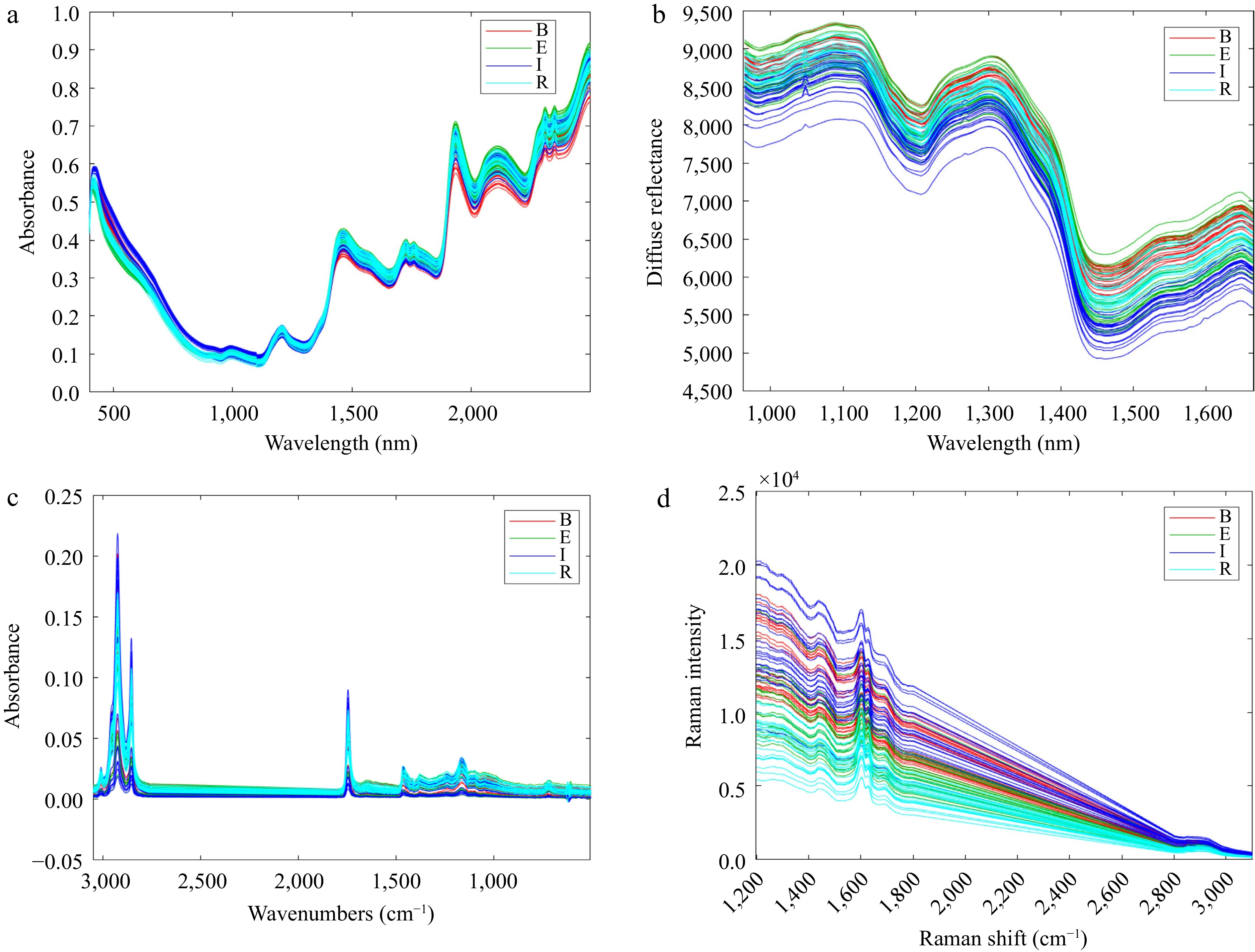
Figure 1.
Raw spectra from instruments before pre-processing data treatment: (a) DG-NIR, (b) HSI-NIR, (c) ATR-FTIR, (d) Raman. GCP samples are labelled according to the country of origin (B: Brazil, E: Ethiopia, I: Indonesia, R: Rwanda).
There are three main issues with spectral data: (i) offsets, (ii) slopes, and (iii) curvature. Offsets are when the spectra are shifted in the y dimension at a constant value, i.e. the entire baseline of a spectrum is offset from zero. Offsets happen when particles are not ground sufficiently or due to an instrumental drift. Offsets were not observed for any of the four instruments (Fig. 1). Slopes are observed in spectra lifted at an inconsistent value slowly across the spectral range[18]. This is observed in Fig. 1d in the Raman spectra and is characteristic of a strong fluorescence effect. Curvature is observed when spectra are lifted at an inconsistent value resembling a curve shape. This was observed in Fig. 1a and b for both the dispersive and hyperspectral NIR systems and is the result of non-linearities introduced by light scatter. It is self-evident that the four data sets have different challenges to mitigate and must be considered in relation to the measurement techniques, which are all based on fundamentally different mechanisms.
Diffusely reflected light is reflected in a broad range of directions and is the primary source of information for NIR spectra[19]. However, diffusely reflected light contains not only chemical information about the sample (absorption), but also the microstructure (scattering). These are Rayleigh and Lorentz-Mie scattering for various reasons, i.e., surface roughness, droplets, crystalline defects, cells, fibers, and density fluctuations. These undesirable light scatter effects and differences in effective path length of light result in baseline shifts (multiplicative) and non-linearities (Fig. 1a & b).
Similar to NIR, ATR-FTIR contains systematic variation due to instrument drifts, sample particle size, etc. Also, samples in the solid state are harder to measure as there needs to be good contact between the crystal and the sample for high surface homogeneity to ensure a representative and accurate measurement.
The strong fluorescence effect observed from coffee has remained a barrier to observing weaker spontaneous Raman signals (Fig. 1d). Few studies have applied Raman spectroscopy to the study of coffee to discriminate varieties[20−22] and monitor changes in coffee quality with time[23]. Various wavelengths and laser power intensities were explored on green coffee powder (GCP) and roasted coffee powder (RCP) with success at collecting Raman signals only using the lipid fraction of GCP at 785 nm[24]. Aqueous extracts of GCP and both aqueous and lipid extracts of RCP were found to have too much fluorescence interference[24]. Other studies discriminating Arabica and Robusta varieties have used the lipid fraction of GCP using Fourier Transform-Raman at 1,064 nm and dispersive Raman at 532 nm[20−22]. To the best of our knowledge, no study has investigated the analysis of green coffee using Raman for the discrimination of coffee origin and using pre-processing techniques to mitigate the fluorescence effect and enhance the Raman signals captured (Supplemental Table S1).
After visually assessing the spectra, only mean centering was applied as a pre-processing step to all four data sets prior to principal component analysis (PCA). For prediction data, high KNN distances indicate samples that appeared in regions that were not sampled well by the calibration data and, thus, are not expected to produce accurate predictions. For all four datasets, all the analytical replicates had KNN = 1 and lower, indicating that no spectral measurements were outlying. For reduced Hotelling's T2 and reduced Q residuals, a 95% confidence interval criterion was set for which an observation is considered an outlier. High reduced Q residuals are observations not well described by the model, while high reduced Hotelling's T2 are observations far from usual observations (score = 0). Most observations fell within the 95% confidence limit for the reduced Hotelling's T2 and reduced Q residuals, with only between 0.04%−1.42% of observations with higher reduced Q residuals. No samples were removed as outliers in the initial exploratory analysis.
Data pre-processing and decision parameters
-
Mathematical relationships between class and spectra must be calculated before spectral data can be used to predict sample classes. The development of these mathematical relationships requires decisions regarding wavelengths and pre-processing methods and considerations of instrument differences. The complex and heterogeneous composition of food and biological systems can lead to considerable variation in the signal-to-noise ratio, which may interfere with the data interpretation of these vibrational spectroscopy tools. Appropriate mathematical pre-processing methods need to be applied to the raw spectral data to ensure that non-uniformity in the size of particles and instrumental errors are accounted for[5], thereby enabling more accurate and robust chemical information to be elucidated. The literature has mainly adopted Raman pre-processing methods from well-established quantitative spectroscopic methods such as infrared spectroscopy. Various pre-processing techniques have been established, including baselining, normalisations, scatter corrections, and spectral derivation. Because these methods have fundamentally different mechanisms, the pre-processing methods adopted successfully towards one dataset may not offer the same benefits for another. The choice of pre-processing needs to be made from understanding the features present in each dataset and how pre-processing affects these features. In addition to statistics to assess the model fit, confusion matrices are typically used in classification problems to represent the quality of the prediction but can be hard to communicate. Accuracy and F1 scores are commonly used (Supplemental Table S1). Matthew's Correlation Coefficient (MCC) may overcome the limitations of accuracy and F1 when dealing with unbalanced datasets and provide a simple yet comprehensive summary of the confusion matrix. The four different instruments and the best pre-processing treatments chosen based on various decision parameters are shown in Table 1. These are summarised in Supplemental Table S1.
Table 1. Prediction statistics associated with optimal pre-processing methods for spectral data collected using DG-NIR, HSI-NIR, FTIR and Raman.
Optimised pre-processing TVar % RMSECV RMSEC RMSEP MCC, Pred. Accuracy, Pred F1, Pred. DG-NIR MNCN 98.54 0.338 0.329 0.473 0.383 0.665 0.483 MSC, MNCN 91.49 0.245 0.243 0.309 0.774 0.882 0.865 SNV, MNCN 91.49 0.245 0.243 0.309 0.774 0.882 0.865 SNV, Detrend, MNCN 91.32 0.245 0.243 0.309 0.774 0.882 0.865 MSC, SG (1st der, 2nd poly, 15 pts), MNCN 76.06 0.268 0.265 0.350 0.684 0.835 0.788 Normalisation, SG (2nd der, 2nd poly, 7 pts), MNCN 98.05 0.358 0.352 0.351 0.652 0.812 0.757 EMSC, MNCN 87.87 0.240 0.238 0.250 0.876 0.929 0.916 HSI-NIR MNCN 99.69 0.372 0.362 0.421 0.618 0.800 0.681 Normalisation, MNCN 98.28 0.333 0.322 0.402 0.655 0.767 0.650 SG (1st der, 2nd poly, 15 pts), MNCN 68.87 0.341 0.325 0.364 0.636 0.800 0.728 MSC, SG (1st der, 2nd poly, 15 pts), MNCN 63.41 0.338 0.324 0.403 0.473 0.733 0.605 Normalisation, SG (1st der, 2nd poly, 15 pts), MNCN 85.79 0.324 0.313 0.375 0.612 0.800 0.732 SNV, SG( 1st der, 2nd poly, 15 pts), MNCN 63.38 0.337 0.324 0.402 0.473 0.733 0.605 FTIR MNCN 99.69 0.335 0.321 0.386 0.253 0.452 0.200 Normalisation, MNCN 98.17 0.334 0.320 0.391 0.372 0.452 0.179 Normalisation, SG (1st der, 2nd poly, 15 pts), MNCN 97.12 0.402 0.369 0.490 0.141 0.500 0.330 EMSC, MNCN 71.52 0.409 0.384 0.482 0.286 0.500 0.326 Raman MNCN 99.91 0.319 0.312 0.329 0.756 0.860 0.819 SG (2nd der, 2nd poly, 7 pts), MNCN 99.66 0.350 0.343 0.369 0.521 0.735 0.648 Normalisation, SG (1st der, 2nd poly, 15 pts), MNCN 98.94 0.321 0.315 0.334 0.554 0.747 0.622 WLS (2nd poly), MNCN 96.86 0.343 0.336 0.372 0.611 0.795 0.760 FT, Fourier-Transform; DG, Dispersive; HSI, Hyperspectral Imaging; NIR, near-infrared; TVar, Total explained variance; RMSE(C/CV/P), Root Mean Square Errors of Calibration/Cross-Validation/Prediction; MCC, Matthew's Correlation Coefficient, MNCN, Mean centering; MSC; Multiplicative Scatter Correction; EMSC, Extended Multiplicative Scatter Correction; SG (#der, #poly, #pts), Savitzky-Golay #derivative, #polynomial, #window points; WLS, Weighted Least Squares; Pred., Prediction. For DG-NIR, all pre-processing treatments beyond MNCN alone showed high accuracy (0.812−0.929) and F1 scores (0.757−0.916), which suggested that the model was performing well (Table 1). However, using Matthew's Correlation Coefficient (MCC) as the decision parameter led to a much lower score for specific pre-processing treatments, e.g., normalisation, Savitzky-Golay (SG) and mean-centering (MNCN) led to a high accuracy of 0.812 but a low MCC of 0.652. This means that the model was not accurately predicting positive (belonging to class) and negative (not belonging to class) outcomes with the same accuracy; belonging to a class was better predicted. MCC considers the dataset imbalance and summarises the confusion matrix as a correlation coefficient[17]. The same observation was found for the HSI-NIR classification models, with all pre-processing treatments showing relatively high accuracy (0.733−0.800) and moderate F1 scores (0.605−0.728) but significantly lower MCC (0.473−0.655). This indicates that the model was poorly predicting sample class origins for HSI-NIR data. Accuracy was consistently the most lenient of the decision parameters compared to F1 scores, which consider the negative and positive aspects of the confusion matrix (false negatives and false positives). Due to having collected a few more analytical replicates for some samples, MCC proved to be a better decision parameter when choosing the optimised pre-processing technique, which considers the number of samples from each class. MCC provided a good summary of the confusion matrix to represent the quality of the class prediction, which is in agreement with a recent statistical study that used MCC as a vital model decision parameter[16]
Another way to test for model performance is to understand the model fit. For that, it has been suggested that the RMSECV and RMSEC values are similar or that the chosen models have low RMSEP values[9]. Typically, the number of latent variables (LVs) in each model is decided using the evolution of root mean square errors of calibration (RMSEC) and root mean squared errors of cross-validation (RMSECV) by the number of LVs used to create the prediction model. Model performance was assessed using RMSEP, as using RMSEC can lead to overly optimistic results.
The following four sub-sections summarise the influence of the top three pre-processing treatments for each vibrational spectroscopy tool. A comprehensive comparison can be found in the supporting information section (Supplemental Table S2). These pre-processing treatments were chosen based on the vital decision parameters MCC and RMSEP on the prediction of each class and the total variance captured by the model. Short descriptions of the influence of each pre-processing step in dealing with spectral interferences are made.
Dispersive near-infrared spectra (DG-NIR)
-
The best pre-processing treatment for dispersive NIR was extended multiplicative scatter correction (EMSC) with mean-centering (MNCN). Multiplicative scatter correction (MSC) and standard normal variate (SNV) processed independently with MNCN were found to provide equivalent results (Supplemental Table S2). Ethiopia (E) and Rwanda (R) consistently had the lowest MCC and highest RMSEP across all four countries. When processed with MSC and SNV, Ethiopia and Rwanda had low MCC (0.511 and 0.584) and high RMSEP (0.408 and 0.378), respectively. Pre-processing with EMSC improved the MCC (0.872 and 0.632) and RMSEP (0.306 and 0.389) scores across Ethiopia and Rwanda. This could suggest that the model was more successful at continental classification across South America (Brazil), Asia (Indonesia) and Africa (Ethiopia, Rwanda).
The results from MSC and SNV agree with previous authors who found a high correlation, 0.995, between the two pre-processing treatments when coupled with MNCN[6]. MSC and SNV are scatter correction techniques, the most common form of pre-processing technique used for near-infrared coffee data (Supplemental Table S1). MSC and SNV mitigate the light scattering effects due to particle size inconsistencies, ensuring that absorption signals are more closely related to chemical constituents of interest rather than scattering artifacts (refer to materials and methods section). EMSC corrects for the curvature observed in Fig. 1a, which likely explains why EMSC pre-processed spectra result in a better classification model. EMSC remains a relatively underutilised pre-processing treatment for NIR coffee studies, with only one author adopting it for identifying coffee bean species using FT-NIR[36] (Supplemental Table S1).
In addition to the aforementioned decision parameters, the model performance can be assessed visually by looking at the scores plot and loadings to determine if the models are indeed modelling differences across our samples based on their chemical differences.
MSC and SNV with MNCN provided equivalent results with 91.49% variance captured by the first two latent variables (Fig. 2bi & bii). Brazil was separated on LV1 (51.16% explained variance) and was characterised by negative scores. Ethiopia and Rwanda are overlapped on both LV1 and LV2. The two African continents are separated from Indonesia on LV2 (40.33%). Pre-processing with EMSC led to an improved continental classification (Fig. 2biii), as evidenced by the scores plot.
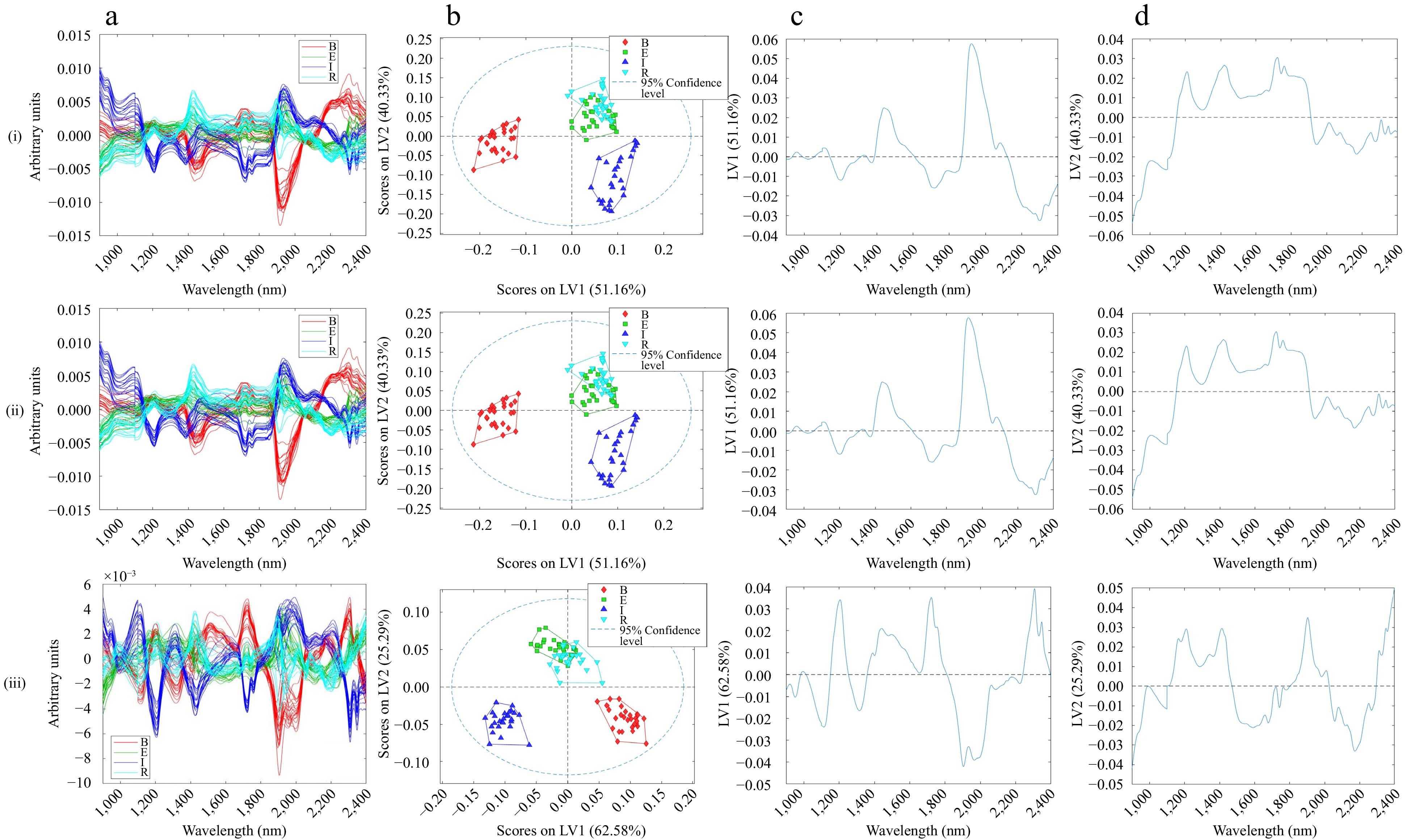
Figure 2.
(a) Pre-processed DG-NIR spectra, (b) scores, (c) first loading, (d) second loading of (i) MSC with MNCN, (ii) SNV with MNCN, (iii) EMSC with MNCN pre-processed DG-NIR spectra.
To relate the distribution of scores to spectral features, the loadings plot of LV1 and LV2 showed that certain spectral regions had corresponding loadings values far from zero. This suggests that these spectral regions are important in explaining the variance of samples on both LV1 and LV2. SNV and MSC pre-processed loadings appear similar, with highly positive loadings for LV1 at 1,400 and 1,950 nm, indicating a difference in water content between Brazil and the other samples. Noting that all the samples were treated the same suggests that there might be differences in water-holding capacity or O-H bonds, typically dominated by water. The loadings for EMSC pre-processed spectra differ from MSC/SNV due to the curvature correction, explaining differences in MCC. There are now two peaks around 1,900 nm, which indicate more than just a water content difference across the samples but also signal the C-H bonds of caffeine[25]. There is a positive peak at 1,200 nm relating to lignin, fatty acids, and amino acids, as well as 2,300–2,350 nm peaks associated with cellulose[37].
Hyperspectral imaging (HSI-NIR)
-
Like DG-NIR, HSI-NIR spectra also showed the need for a baseline correction to correct the curvature observed (Fig. 1b). DG-NIR incorporated a higher wavelength range, unlike HSI-NIR, which only recorded a range of 900–1,700 nm, and the HSI-NIR raw spectra were noisier than the DG-NIR raw spectra. To correct for the curvature, EMSC, MSC and SNV were explored (Supplemental Table S2), but they failed to improve the classification. Savitzky-Golay derivatives (SG) were explored to remove additive and multiplicative effects in the spectra. The first derivative only removes the additive baseline effect, while the second derivative also removes the linear trend (multiplicative effects). When the spectra were pre-processed with 1st derivative SG (15 window points, 2nd polynomial) and MNCN, the model captured a moderate classification with 68.87% variance. Accuracy was moderate at 0.729 with a lower F1 score of 0.675 and a much lower MCC of 0.486; this model prediction was not good. Normalisation with 1st SG (15 pts) derivation and MNCN (85.79% variance captured) had a slightly better classification with an accuracy of 0.760 and an F1 score of 0.701. However, the MCC was still low at 0.567. Similar to DG-NIR, the Ethiopian and Rwandan samples had the lowest MCC and highest RMSEP compared to the other classes, as the model was more successful at continental separation. Normalisation with MNCN performed similarly to MNCN spectra. However, the classification was based on the baseline effects not removed with pre-processing, as shown in Fig. 3ci below.
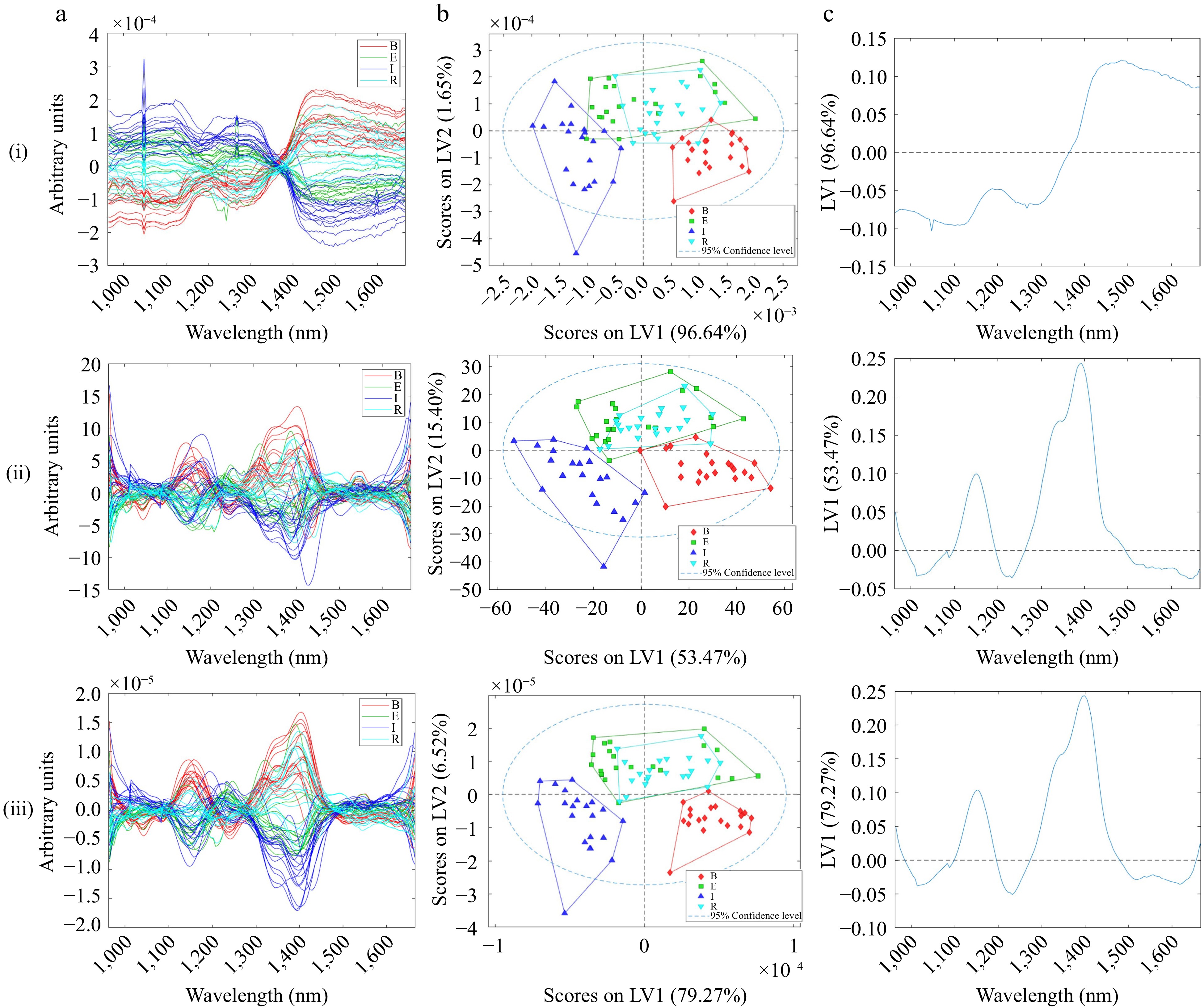
Figure 3.
(a) Pre-processed HSI-NIR spectra measured in reflectance, (b) scores, (c) first loading of (i) Normalisation with MNCN, (ii) SG (1st der, 2nd poly, 15 pts) with MNCN, (iii) Normalisation, SG (1st der, 2nd poly, 15 pts) with MNCN pre-processed HSI-NIR spectra.
The scores plotted in Fig. 3bi were pre-processed with normalisation and MNCN. The model performs similarly to the other two models with continental separation, capturing 98.28% of the variance across samples. However, the loadings plot in Fig. 3ci indicates that the model is classifying the samples due to baseline influences. This demonstrates that normalisation alone could not mitigate the unwanted physical artifacts. With reference to Fig. 3bii, pre-processing with SG (1st der, 15 pts) with MNCN had moderate continental classification, but the model only captured a total of 68.87% of the variance across the samples. This is because the pre-processing has mitigated the baseline variance. Similarly, pre-processing with normalisation, SG (1st der, 15 pts), and MNCN led to a similar model performance with 85.79% variance captured by the model on the first two latent variables. However, comparing the latter two models, the RMSEP and MCC were better for the model pre-processed with SG (1st der, 15 pts) and MNCN, particularly for the Ethiopian and Rwandan samples. Figure 3cii shows that the model classifies the samples according to the desired wavelength associated with chemical differences. The NIR spectra collected from the hyperspectral imaging system are characterised by absorption bands related to lignin, fatty acids, and amino acids between 1,100−1,300 nm and cellulose O-H bonds at 1,450 nm[37]. Comparing the loadings of DG-NIR and HSI-NIR, the regions of importance are the same. However, it was also found that loadings of DG-NIR at the higher NIR region were also important for classification; specifically, the loadings at 1,900 nm are associated with caffeine, and around 2,300 nm are associated with cellulose (Fig. 2ciii). It must be noted from Fig. 3ai that there was a bad pixel in the detector at about 1,050 nm. The bad pixel had a minor influence on the model but could be dealt with through a median smooth[26,27].
Overall, HSI-NIR performed worse than DG-NIR. This could be attributed to the low number of regions of interest (ROI) points chosen (7–9/sample). A larger dataset to calibrate the model on may help improve the performance. A similar study using HSI-NIR (900–1,700 nm) to discriminate the origins of 120 samples of green tea powder coming from three regions within Chongqing, China, performed exceptionally well at 90% accuracy with PLS-DA. This could be attributed to the higher number of samples within each origin class[28]. Better model performance from DG-NIR could also be attributed to the wavelengths not measured in hyperspectral, such as between 1,850–2,350 nm, which signal absorptions belonging to caffeine and hemicellulose, which may be necessary for classifying the coffee samples. This is the first study comparing the sensitivity of HSI-NIR with DG-NIR for origin discrimination in coffee. Further studies are needed to confirm the selected wavelength regions that are important for origin discrimination.
Mid-infrared spectra (FTIR)
-
The initial data exploratory step with PCA did not indicate a potential successful classification. The raw spectra did not appear to require any form of pre-processing, given that no offsets, slopes or curvature were observed (Fig. 1c). Nonetheless, the typical pre-processing steps used for FTIR data were conducted systematically (Supplemental Table S1) to understand the influence of pre-processing. Differences in contact or density of the sample could lead to a lower potential signal. Normalisation may mitigate this effect[29−31]. Differentiation using Savitzky-Golay (SG) is typically done to suppress unwanted signals and backgrounds or even separate overlapping peaks[32,33].
The model accuracies, F1 and MCC scores were generally extremely low, informing us that the model was not working well to predict coffee sample origin, and often at a rate of chance. While pre-processing can substantially improve the final model performance, as evidenced by the NIR dataset, sample preparation is also critical to a good predictive model. The FTIR measurements were obtained using an ATR diamond accessory. This required intimate contact across the powder and the diamond crystal, which is characteristically hard to achieve and ensure reproducibility. Some of the green powder formed lumps while awaiting analysis, and a pestle and mortar were used to remove the lumps and ensure no air gaps while packing the powder onto the crystal. There was no significant water peak in the FTIR spectra, which did not affect the infrared signals. It must be noted that the classification regions were explored at a limited region of between 600–1,800 cm−1 and 2,750–3,050 cm−1 to remove the noise region. These regions were also selected by other researchers looking at origin discrimination of five country GCBs using ATR-FTIR and PCA[30]. Another study comparing NIR and ATR-FTIR found better model accuracy using ATR-FTIR, but the study looked at regions within Brazil[32]. This disagreed with the findings from this study, which showed better results using NIR, which could be attributed to the differences in origin scales (country vs region).
Raman spectra
-
The slope shown in Fig. 1d is characteristic of the fluorescence effect, which hinders the extraction of the weaker Raman signals, as demonstrated by previous coffee researchers[20−24,34,35]. To deal with the influence of artifacts in Raman spectra, pre-processing treatments like those used for IR spectra are typically used (Supplemental Table S1). Normalisation and baseline correction have also been examined[34,35]. In this study, we attempted pre-processing treatments typically used for IR spectroscopy and a weighted least squares treatment. The spectral regions explored were limited to 1,200–1,800 cm−1 and 2,800–3,100 cm−1 to remove the noise regions. The PCA scores plot indicated partial continental separation after mean centering was applied. Similar to NIR data, Ethiopia and Rwanda were found to be worst predicted according to MCC and RMSEP (Supplemental Table S2). Pre-processing improved the MCC scores for Indonesian samples, and the values for decision parameters were quite comparable. The accuracy and F1 values across the top three pre-processing steps appear to be quite similar, reinforcing the need for MCC as a decision parameter. PLS-DA model with MNCN appeared to have relatively good scores separation of the country of origin, but the loadings plot indicated that the samples were being modelled by the variance due to the fluorescence (slope). The slope mirrors the 785 nm Raman results from a study on GCP oils for quality control[24]. This highlights the potential for fluorescence to be useful for coffee origin classification. To understand if pre-processing treatments were able to mitigate the observed slope, we look at the scores and loadings plot in Fig, 4.
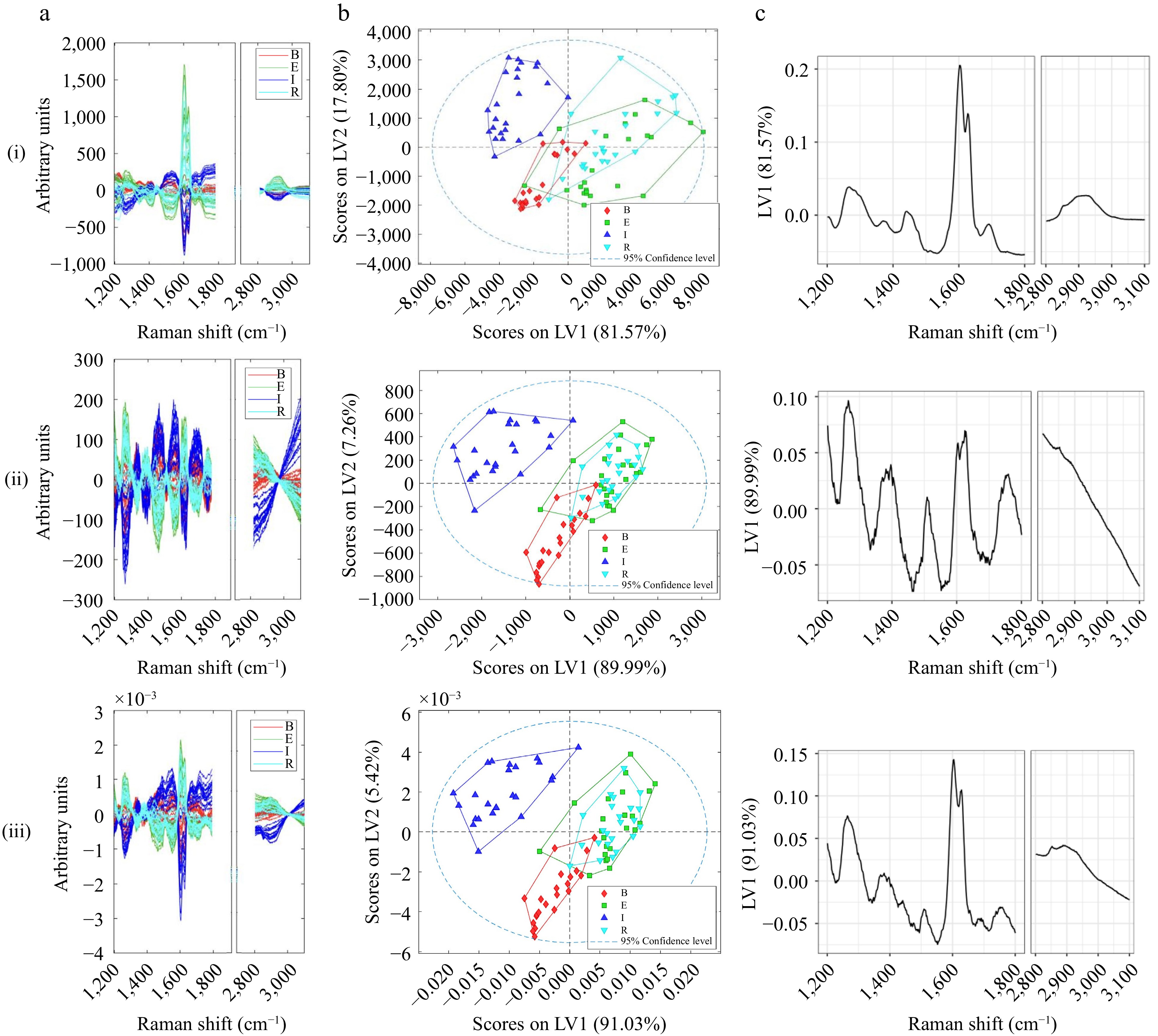
Figure 4.
(a) Pre-processed Raman spectra, (b) scores, (c) first loading of (i) MSC with MNCN, (ii) EMSC with MNCN, (iii) WLS, Normalisation with MNCN pre-processed Raman spectra. Loading plots were produced using R.
With reference to Fig. 4c, all three pre-processing techniques appear to have mitigated the fluorescence effect (slope) to allow the Raman shift associated signals to be elucidated. Pre-processing with WLS and normalisation appeared to provide the clearest continental separation (Fig. 4biii). Normalisation per unit vector length helped to reduce the systematic variations[22], while weighted least squares (WLS) subtracts the baseline from a spectrum using an iterative asymmetric least squares algorithm. To correlate the Raman shifts to the chemical constituents, the loading plot between 2,800 and 3,100 cm−1 are attributed to symmetric and asymmetric C-H stretching vibrations, while the signals between 1,200 and 1,800 cm−1 are related to typical organic groups, which have also been found to be relevant to the discrimination of coffee species and considered the fingerprint of the samples[24]. Specifically, bands at 1,478 and 1,567 cm−1 are related to kahweol, 1,693 cm−1 related to C=O stretching[23], and 1,657 cm−1 with C=C stretching of polyphenols and chlorogenic acids[20,35]. Given its fluorescence effect, Raman has not been used in the literature for origin discrimination. Nonetheless, the wavelengths found to be important for origin discrimination mirror the regions found by Dias & Yeretzian[24]. Further studies are needed to confirm the Raman wavelength regions contributing to origin discrimination and the potential of the fluorescence effect to be modelled.
-
To optimise the pre-processing step, decision parameters must be well chosen. Matthew's Correlation Coefficient (MCC) appears to be a useful metric to establish the performance of a classifier in the confusion matrix for the optimisation of vibrational spectroscopy tools. This study has shown the reliability of vibrational spectroscopy tools, which are rapid, cost-effective, and sustainable solvent-less solutions for the geographic origin traceability of coffee. Near-infrared was the most reliable instrument, considering the ease of use, sample preparation and model performance. The dataset used to compare these instruments was small. Future studies with a wider range of sample sets covering different coffee batches and seasons and an external validation set should lead to more robust and stable classification models. Future studies can look at the potential of hyperspectral near-infrared for the origin traceability of whole intact coffee beans and hyperspectral instruments with broader wavelengths. The easily automated protocols and vibrational spectroscopy tools coupled with advanced machine learning may soon become empowering tools for coffee producers to protect themselves.
-
The authors confirm contribution to the paper as follows: conceptualisation, investigation, methodology: Sim J, McGoverin C; data analysis, visualisation, writing - original draft & editing: Sim J; data curation: McGoverin C; supervision: Oey I, Frew R, Kebede B; writing - review & editing: McGoverin C; Oey I, Frew R, Kebede B. All authors reviewed the results and approved the final version of the manuscript.
-
The datasets generated during and/or analyzed during the current study are available from the corresponding author on reasonable request.
-
We acknowledge the support of time and facilities from the University of Auckland, Department of Physics, Oritain Global Ltd., and the University of Otago Department of Food Science technical support staff for help in this study. We acknowledge permission from Oritain Global Ltd. to submit this manuscript for publication. We acknowledge the assistance of Samer Naji with a part of the data collection. We would also like to acknowledge the University of Otago for the Doctoral Scholarship.
-
The authors declare that they have no conflict of interest. Indrawati Oey is the Editorial Board member of Food Innovation and Advances who was blinded from reviewing or making decisions on the manuscript. The article was subject to the journal's standard procedures, with peer-review handled independently of this Editorial Board member and the research groups.
- Supplemental Fig. S1 Energy diagram of Raman and IR spectroscopy mechanisms with numbers .representing the different vibrational levels within each electronic state.
- Supplemental Table S1 Overview of the most common vibrational spectroscopy instruments, their principles, pre-processing and model parameters used by researchers investigating coffee.
- Supplemental Table S2 Optimised pre-processing and decision parameters for (1) DG-NIR, (2) HSI-NIR, (3) FTIR, (4) Raman.
- Copyright: © 2024 by the author(s). Published by Maximum Academic Press on behalf of China Agricultural University, Zhejiang University and Shenyang Agricultural University. This article is an open access article distributed under Creative Commons Attribution License (CC BY 4.0), visit https://creativecommons.org/licenses/by/4.0/.
-
About this article
Cite this article
Sim J, McGoverin C, Oey I, Frew R, Kebede B. 2024. Optimisation of vibrational spectroscopy instruments and pre-processing for classification problems across various decision parameters. Food Innovation and Advances 3(1): 52−63 doi: 10.48130/fia-0024-0004 

Optimisation of vibrational spectroscopy instruments and pre-processing for classification problems across various decision parameters
- Received Date: 11 December 2023
- Accepted Date: 15 March 2024
- Published Online: 29 March 2024
Abstract: Vibrational spectroscopy is a green, rapid, and affordable analytical tool for analysing the quality, safety, and origin of biological materials in agri-food sectors. Pre-processing spectral data is crucial to removing instrumental interferences and physical artifacts when developing a classification model. However, there has yet to be a consensus on which spectral pre-processing method, settings, and decision parameters to use to optimise pre-processing for different spectroscopy tools. Using an arbitrary criterion poses a risk of applying the wrong type or too severe pre-processing that removes valuable information or affects the model's performance for prediction studies. Matthew's Correlation Coefficient (MCC) - a statistic for parameterising classification performance, accounts for data set imbalance and improved decisions on model selection to express uncertainty on future predictions. Four vibrational spectroscopy instruments [near-infrared (NIR), hyperspectral (HSI), mid-infrared (FTIR), and Raman] were compared using different pre-processing methods to understand the performance using MCC to classify coffee from four countries (Indonesia, Ethiopia, Brazil and Rwanda). Key decision parameters were evaluated for the development of reliable classification models. The best pre-processing for NIR was extended multiplicative scatter correction with mean centering (MNCN), and for HSI, Savitzky-Golay (1st derivative, 15 points) with MNCN. NIR performed the best across all four instruments, with FTIR performing the worst. Raman showed potential for coffee origin classification using the right pre-processing. Pre-processing with weighted least squares, normalisation, and MNCN eliminated the fluorescence effect on Raman spectral data. These findings show the feasibility of using MCC for classification problems.
-
Key words:
- Vibrational spectroscopy /
- Chemometrics /
- Pre-processing /
- Model optimisation /
- Decision parameters