Kennedy Munene Ondieki
Strathmore Institute of Mathematical Sciences, Strathmore University, Nairobi, Kenya.
DOI: 10.4236/jmf.2022.122024   PDF    HTML   XML   170 Downloads   1,020 Views   Citations

Abstract

The thesis seeks to use simulated annealing optimization to minimize the difference between the value of the libor model volatility and the ones quoted in the market for congruent pricing of a Swaption contract. The simulated annealing optimization technique, being a global minimisation method, would provide accurate parameters that will simulate libor rates that are harmonious with the observed yield curve. This latter feature employed in a Monte-Carlo pricing method would price the Swaption contract fundamentally closer to its market value than other local optimization methods. The SA method starts from an initial point, often random, then searches the neighbourhood of the current solution for the next point. The neighbourhood function search is in accordance with the set probabilistic distribution that will determine the distance between the two solutions. Each solution has a cost value associated with it. The cost function determines the eligibility of the solution by measuring its discrepancy with the set limit. If the discrepancy is larger than the set limit, a new solution is sought. If the discrepancy is still large, the old and new cost value is compared, and the latter is accepted if it’s less than the former or otherwise rejected with a certain probability that is largely dependent on the control mechanism. The method terminates if the cost value attained is equal to the set tolerance level. Different from other heuristic methods that solely base their solution on the iterative improvement of the solution’s cost value, simulated annealing accepts some inferior solutions so as to have a wider search in the design space. The main advantage of the method is the ability to escape local minimum entrapment through the aforementioned acceptance/rejection criteria. The results indicate that the advantageous aspects of the Simulated annealing enable it to outperform the least square non-linear optimization method commonly used in the simulation.

Keywords

Swaption Pricing, Monte-Carlo Method, Simulated Annealing, Annealing Function, Acceptance/Rejection Criterion

Share and Cite:

1. Background of the Study

Swaptions are options that give the holder the right but not the obligation to enter into a swap contract on a future date at a pre-agreed strike rate. A swap contract is an agreement between two parties to exchange a floating and fixed interest rate payment for a tenor. The interest rate payments are based on the same notional amount which is not exchanged. The exchange involves one party paying the other the net value of the two payments on scheduled dates. In the option, the holder who agrees to pay the fixed rate in the swap and receive the floating rate is the payer swaption, whereas the holder who agrees to pay the floating rate and receives the fixed is the receiver swaption. A payer swaption would exercise the option if the swap rate is higher than the option strike and the receiver swaption would exercise if the latter is higher.

There are various reasons to enter into a swaption contract, with the most common one being to transform the nature of an asset’s interest rate payments. By buying a receiver swap, the holder can transform the interest rate applicable to an asset from a floating to a fixed rate, hence hedging against interest rate risk. Since the contract is an option, it is expected to be exercised only if the payoff is positive. The other prominent reason would be to speculate against the interest rate cycle. If a firm was to expect a fall in the interest rate in the near future, they could enter into a receiver swaption to take advantage of the high fixed rate as the floating rate plumber.

There has been a significant increase in the trading of interest rate swaps over the past half-decade, which has led to the expansion of its option derivative.

Recent surveys indicate that the market turnover for swap options as of 2016 was $163.021 trillion, and the figure went up to ([wooldridge2019fx:01]). In March 2021 particularly, [1] reports that USD swaptions volume hit an all-time high i.e. 6346, which was on the back of a record month in February 2021, when 5973 trades were reported. The volume was driven by a large sell-off in fixed-income markets. This substantiates the importance of proper hedging and pricing formulae in order to value the contracts accurately. Good pricing performance is a necessary condition for a useful model; good hedging performance, however, is sufficient [2] .

Markets always quote swaptions volatilities in a periodic series of either 3, 6, or 12 months, hence a more direct pricing strategy would be to model applicable libor rates with same time discretization as opposed to modelling the instantaneous rate and then prorating the forward rates applicable over the periods. This makes the market models like the libor process more empirically suitable to model the forward rates applicable in swaptions.

Market models have become popular in pricing basic interest rate derivatives namely caps and swaptions because of their agreement with well-established market formulas i.e. Libor-forward rates (LFR) prices caps with Black’s formula whereas libor swap rates (LSM) prices swaptions with same the formula. However, LFR and LSM are not compatible with each other in theory, but empirically their distribution is not far off each other. Nevertheless, we shall adopt the LFR model to price swaption because they are more natural representative coordinates of the yield curve than the swap rates. Additively, it is natural to express the LSM in terms of a suitable preselect family of LFR rather than doing the converse [3] .

The pricing of swaptions hinges on the LFR process with parameters that are optimized in accordance with the market volatilities of existing interest rate products. Through the transformation of Black’s formula, traders extract implied volatilities from tradable assets, which are then used to derive LFR’s dynamics for simulation.

Optimization provides an excellent method to select the best element in terms of some system performance criteria from some set of available alternatives. On the other hand, a simulation is a tool that allows us to build a representation of a complex system in order to better understand the uncertainty in the system’s performance. Often the emphasis is put on simulation, leaving optimization techniques at the discretion of the trader. Sometimes the optimization technique used leads to large errors that significantly affect the simulation and hence the model performance. When considered separately, each method is important, but limited in scope. By giving the two equal weights, we can develop a powerful framework that takes advantage of each method’s strengths, so that we have at our disposal a technique that allows us to select the best element from a set of alternatives and simultaneously take account of the uncertainty in the system.

Swaption pricing has often adopted the least-square non-linear (lsqnonlin) method to minimize the error between the model parameters and the market measures. The method is computationally easy to use but it can get trapped in the local minimum, hence greatly overestimating the parameters. The method’s major drawback is that it doesn’t have any known mechanism to get out of local minimum entrapment. Local minimum parameters would have much higher errors than global minimums if the two are not one and the same.

Simulated annealing (SA) optimization searches the global minimum parameters by utilizing a probabilistic transition rule that determines the criteria for moving from one feasible solution to another in the design space. Sometimes the rule accepts inferior solutions in order to escape from local minimum entrapment. This enables it to search higher dimensions for other minimum points, and in the process converge to the global minimum. The method also doesn’t require any mathematical model making it suitable for problems that do not have an exact distribution [4] .

2. Simulated Annealing Overview

Simulated annealing optimization imitates the annealing process used in metallurgy whereby a substance is heated to its melting point and then it is slowly cooled in a controlled manner until it solidifies. The process largely depends on the cooling schedule to determine the structural integrity of the resultant substance. If the cooling is too quick, the substance forms an irregular crystalline lattice hence making it weak and brittle. If the cooling is slow the substance formed is strong since the crystal lattice is regular.

SA establishes the link between the thermal cooling behaviour and searches for the global minimum. The resultant substance with a regular crystalline lattice represents a codified solution to the problem statement and the cooling schedule represents how and when a new solution is to be generated and incorporated. The technique has basically three steps; if the old solution doesn’t meet the set requirements, perturb it to a new one, then evaluate the new solution given the old one, and finally accept or reject the new solution. The analogy of the cooling schedule could be represented using the picture below (Figure 1) [4] .

The objective is to get the ball to the lowest point of the valley. At the beginning of the the process the temperature is high and strong perturbations are exerted on the box and hence the ball can jump through the high peaks in search for the bottom of the valley. As the time goes by and the temperature reduces, the perturbations become weak hence the ball can only jump small peaks. At the time the temperature reduces to very low levels, there is a high probability that the ball will be in the lowest depression of the valley. In the algorithm, the temperature forms part of the controlling mechanism for accepting a new solution i.e. When the the temperature is high, the SA optimization is searching for the global solution in a broad region, but as the temperature reduces the search

radius reduces hence refining the feasible solution attained at high temperatures.

The algorithm uses the solution error to evaluate the eligibility of the new solution. The solution error is calculated from the objective function to be optimized. Usually each solution $X_i$ is associated with its error $E_i$ . The error is used to evaluate the new solution by determining its acceptance or rejection. If the error in the new solution is less than the old, it is automatically accepted, on the other hand if it is more it accepted but under a set probability ( $P_n$ ) i.e.

$P_n=(\begin{array}{ll}{\exp }^{-\frac{k\Delta E}{T}}\hfill & \Delta E\ge 0\hfill \\ 1\hfill & \Delta E\le \mathrm{0,}\hfill \end{array}$

where $\Delta E$ is the change in the solution error after it has been perturbed, T is the current temperature and K is a suitable constant. Through the acceptance/rejection criteria above, the algorithm can accept inferior solutions but the probability reduces as the temperature reduces or as the $\Delta E$ increases. Consequently, at high temperatures the algorithm searches a broad area hence accepts bad solutions, as the temperature reduces, the algorithm is more selective and only accepts solutions when the $\Delta E$ is very small. The algorithm termination criteria is user defined and mainly include error tolerance level, maximum number of iteration, or attained temperature level.

The algorithm components include; a neighborhood function that conducts the perturbations, a cooling function that dictates how the temperature reduces and an acceptance function for evaluation of solutions.

SA versatility can be attributed to the feedback generated by its users which has in turn been used to add various options that go beyond the basic algorithm. The power & flexibility accorded by the feedback mechanism has enabled it to be applied across many platforms. In cases where the default options are not applicable, it accepts customized functions. The introduction of re-annealing also permits adaptation to changing sensitivities in the multidimensional parameter-space [5] .

3. Literature Review

Before the libor market model was derived, the difficulty in valuation of caps and swaptions was attributed to presence of unobservable financial quantities like instantaneous forward rate or short rate, in the pricing formulae. This holds major disadvantage in that a transformation via black box in the model is needed in order to map the dynamics of this unobservable quantities to observable ones [6] .

The developments that led the derivation of the Libor process was reported in [7] where it was shown how to choose the volatility functions (and a change of measure), so that libor rates follow lognormal processes. Although it is an extension of Heath,Jarrow & Morton model (HJM), the libor process differs in that the process has observable market quantities and produces well behaved forward rates than HJM’s which can go to infinity in finite time [8] . The hallmark of the model was anchored upon having an arbitrage free process that can accommodate correlated forward rates.

The libor also holds an advantage over the short rate process in that; it can achieve decorrelation of forward rates, the estimated parameters can be interpreted, and it models the forward rate as primary process as opposed to a secondary one. Decorrelation is achieved by finding the most effective way to redistribute the volatility of the libor rates as time lapses [3] .

[9] considered the various implementation methodologies of pricing caps and swaptions in the libor framework. The paper highlights that Monte-Carlo method with parametric correlation matrix has a more stable evolution of volatility and correlation, which is a desired feature in pricing exotic options and also hedging. It also states that non-parametric approach poses minimization problems as the number of free parameters becomes large, hence impossible to estimate since the number of forward rates alive may not be sufficient.

In the libor framework, once time dependent instantaneous volatility and correlation of the forward rates have been specified, their stochastic evolution is completely determined. This leaves the matching of Black’s volatility (path independent) to the integral of instantaneous volatility (path-dependent) the only approximation needed. [10] indicates that by using a self financing strategy between the swaption and the libor rates and assuming that both have lognormal distribution and deterministic volatilities, the Black’s volatility can be approximated by a linear function of swap rates weights, correlation coefficient and instantaneous volatility.

In solving the need for the correlation matrix to have a rank less than the number of factors considered, [6] proposed a discerning parameterization method that uses a hyper-sphere decomposition before dimensionality problem is addressed. However the correlation matrix will depend on the bounds set for the angles. Use of spherical coordinates in the specification of instantaneous volatility allows for a more robust optimization scheme [11] . This methodology will be applied in this thesis.

The basic SA algorithm that was originally published by [12] had two main implementation strategies for the acceptance probability. The primary one was Boltzmann annealing which was credited to Monte Carlo importance-sampling technique for handling large-dimensional path integrals arising in statistical physics problems. The method was generalised so as to fit non-convex cost functions arising in various fields. The acceptance probability is based on the chance of obtaining a new solution error relative to the previous one. The secondary one was fast annealing, which adapted the Cauchy distribution for its acceptance probability as opposed to Boltzmann distribution. In comparison with the Gaussian Boltzmann form, the fast Cauchy distribution has fatter tails hence permits an easier access to test local solutions while searching for the global one.

In the [13] paper, “Theory and practice of Simulated annealing”, they enlist topography and size of the design space as the key variables that need to be considered while choosing the sampling function. A sampling function that imposes smooth topography in cases where the local minima are shallow is preferred to a bumpy one. On the issue of size, the main consideration is the ability of the function to reach other feasible solution in finite number of iteration i.e necessity of reachability. The paper also offer other conjures by hinting that sampling a small size of solution space is preferred as compared to large one because the latter will have the algorithm sampling large portions hence unable to concentrate on specific areas of the design space. Contrary to the suggestion above, a larger annealing sample guarantees a better SA performance than a small one. They also suggest a method of reducing the search space by isolating the strongly persistent variables¹ during SA execution. Ultimately, the function will highly depend on the problem at hand.

Cooling schedules commonly used in SA was originally proposed by [14] . It includes an initial temperature $T_0$ ; which must be too high so that the new solution sought is accepted with probability close to 1, a temperature decreasing function; generally an exponential function with a parameter $\alpha$ , and the number of iterations k for each temperature level before it reduces. [15] describes three temperature reduction function commonly used in empirical application as.

1) Multiplicative Monotonic Cooling—Temperature is reduced by multiplying it with a parameter $\alpha$ . $\alpha$ generally varies from 0.8 - 0.9.

2) Non-Monotonic Adaptive Cooling—Temperature is reduced my multiplying it with an adaptive factor that is based on the difference between the current solution objective.

3) Additive Monotonic Cooling—Two additional parameters are included namely; the number n of cooling cycles, and the final temperature $T_n$ of the system. In this type of cooling, the system temperature T at cycle k is computed adding to the final temperature $T_n$ , a term that decreases with respect to cycle k.

Each has four variants namely quadratic, linear, exponential and logarithmic. Non-Monotonic Adaptive Cooling has also a trigonometric version.

[16] documents the importance of choosing a good initial temperature for the cooling schedule as it determines the ability of the algorithm to find good solutions. In the paper, he gives four accounts of calculating the initial temperature. The first is equating it to the largest cost value difference between any two solutions in the design space. The second equates it to a function of a constant and the volatility of the cost value differences i.e. $k{\sigma }_{\infty }^2$ . Temperature is taken to be at infinity and K is between 5 and 10. The third is coined from the relationship between temperature parameter and the acceptance ratio i.e. starting from a given acceptance ratio ${\chi }_o$ , a large enough temperature is first tested and the ratio is calculated. If the ratio is less than the ${\chi }_o$ , the temperature is multiplied by two, if larger, it is divided by three. He gives the latter method a thumbs up as it is able to avoid cycles and a good estimation of the initial temperature is easily found. The fourth borrows slightly from the former in that the initial temperature is the quotient of the average cost value changes and the logarithm of the set initial acceptance ratio ${\chi }_o$ . The method starts by first generating some random transitions so as to be able to compute the average change of the cost value.

[17] studied the application of SA in stochastic & deterministic optimization whilst using constant and varying sample size. The constant/variable sample is incorporated in the neighbourhood function in that the next solution is evaluated as an average of chosen samples size. He motivates the importance of choosing a good cooling schedule for the temperature parameter in evaluating the neighbourhood solution so as save on computational time and increase efficiency. In his conclusion remarks, the varying sample method performs better for deterministic problems, whereas constant sample performs better for complex stochastic problems.

[18] whilst strived to maximize the expected logarithm utility function, investigated the use of simulated annealing in optimization of wealth allocation of stocks for capital growth problem. The paper adapted a Cauchy function to move from one feasible solution to another. In order to have a positive capital growth, the wealth allocations of the stocks have to be a below a critical point. Since the number of stocks available is numerous, the strategy heavily relies on the weight put on each stock. Any local optimization method will overestimate the parameters consequently affecting the outcome greatly. They showed that by using Cauchy sampling function and decreasing cooling schedule the parameters could escape the local maxima and achieve global maximum parameters with significant accuracy to warrant a positive capital growth.

[19] examined the problem of selecting optimal sparse mean reverting parameters based on observed and generated time series. They adapted SA method and compared it with the greedy method. The paper reports that the SA methods outperform the greedy method in 10% of the cases where the asset’s cardinality is small. The percentage increases to 25 when the assets and cardinality restriction are doubled, indicating that the SA method becomes more attractive for larger assets whilst maintaining asymptotic runtime of simpler heuristics.

[20] compares the various optimization techniques applied in minimization of volatility function in pricing of caps & swaptions in Cheyette model. In his paper he acknowledges the superiority of non-derivative algorithms like downhill simplex or Genetic algorithm in implementation of the model. In his execution, he embedded the downhill simplex method in the SA algorithm. Beyna results indicate lower free parameters than calculated by Downhill simplex method. The paper also tested several cooling annealing schedules i.e. linear, exponential cooling schemes and some adaptive ones. It turned out, that the linear cooling scheme delivers the best results, if the cooling factor is chosen considerably small.

4. Methodology

The libor² process models forward rates which are in turn used to evaluate the expected payoff of swaptions under some measures. The process assumes that the rates follow log-normal distribution so as to be able to recover the [21] formula. In coming up with the formula, the thesis employs Martingale representation method.

4.1. Martingale Representation Method

Martingale is a process that has the property that at each point in time, the conditional distribution for the future point in time is centred around the mean. This constraint on the process stops it from becoming too wild [8] . Martingale representation theorem allows the payoff of interest rate derivatives to be evaluated using an expectation of a stochastic martingale process [22] . Taking the price of an option evaluated with respect to numeraire N or any traded asset with its corresponding probability measure ${\mathbb{Q}}_{\mathbb{N}}$ , to be $C_t$ at timet and the payoff at time T to be $X_T$ , its martingale representation can evaluated as:

$\frac{C_t}{N_t}={\mathbb{E}}^{{\mathbb{Q}}_{\mathbb{N}}}\left[\frac{X_T}{N_T}\mathrm{<mo>\; |\; </mo>}{F}_t\right]\mathrm{,}$ (1)

where:

$X_T=\max \left(R_T-K,0\right).$

4.2. Change of Numeraire

Many computational applications of derivatives pricing models such as determination of derivative prices by simulation or the estimation of derivative pricing models can be significantly simplified by a change of numeraire [8] . The numeraire is chosen so as to simplify the equationi.e. when $N_T$ is stochastic it can’t be factored out, but a change of numeraire can have it change to unit hence easily simplifying the equation³. Radon-Nikodym derivative allows one to make the switch from expectation under one measure to another measure e.g. from T-forward measure to forward swap measure.

4.3. Swaps

Interest rate Swap is an agreement to exchange payments using two different indexes i.e floating and fixed. The party that agrees to pay the fixed and receive the floating index is the Payer swap and the converse is the receiver swap. The fixed index pays a fixed amount K at every instance $T_j$ while the floating side pays $L_j\left(T_{j-1}\right)$ . Different from the fixed rate, the floating have a reset date $T_j$ that stipulates the forward rate applicable at the time of payments $T_{j+1}$ , for the tenor $T_o\cdots T_{\beta }$ , hence the notation $L_j\left(T_{j-1}\right)$ .

Thus, the payoff at time $t<T_0$ of such a payer swap contract denoted as $\text{IRS}\left(t_0,T_0,T_n,K\right)$ can be written as⁴:

$\text{IRS}\left(t_0,T_0,T_n,K\right)=\mathbb{E}{\displaystyle \underset{j=0}{\overset{\beta -1}{\sum }}}D\left(t,T_j\right){\tau }_j\left(L_j\left(T_{j-1}\right)-K\right),$ (2)

where ${\tau }_j$ is the year fraction between $T_j-T_{j+1}$ , $D\left(t\mathrm{,}{T}_j\right)$ is the discount factor, 0 is the commencement date of the contract and $\beta$ is the expiry.

The contract can be evaluated (at time t) under the $T_{j+1}$ forward measure by using the price of the bond maturing at time $T_{j+1}$ as the numeraire, i.e.

$\text{IRS}\left(t_0,T_0,T_n,K\right)={\tau }_j{\mathbb{E}}^{T_{J+1}}{\displaystyle \underset{j=0}{\overset{\beta -1}{\sum }}}\frac{P\left(t,T_{j+1}\right)}{P\left(T_{j+1},T_{j+1}\right)}\left(L_j\left(T_{j-1}\right)-K\right).$ (3)

By assuming that $L_j\left(t\right)$ is a martingale under the $T_{j+1}$ forward measure, we can express the value of the payer IRS as:

$\text{IRS}\left(t_0,T_0,T_n,K\right)={\tau }_j{\displaystyle \underset{j=0}{\overset{\beta -1}{\sum }}}P\left(t,T_j\right){\tau }_j\left(L_j\left(t\right)-K\right).$

The fixed rate that makes the IRS a fair contract at time t, denoted as $R_{\mathrm{0,}\beta }\left(t\right)$ , should be calculated with the condition $\text{IRS}\left(t_0\mathrm{,}{T}_0\mathrm{,}{T}_n\mathrm{,}K\right)=0$ . By setting the expression of the payer IRS equal to zero, the forward swap rate $R_{\mathrm{0,}\beta }\left(t\right)$ may be expressed as:

$R_{0,\beta }={\displaystyle \underset{j=0}{\overset{\beta -1}{\sum }}}{W}_j\left(t\right)L_j\left(t\right),$ (4)

where

$W_j\left(t\right)=\frac{P\left(t,T_j\right)}{{\displaystyle {\sum }_{j=0}^{\beta -1}P\left(t,T_j\right)}}.$ (5)

Equation (4) means that the the forward swap rate is a weighted average of the of the libor rates over the tenor since $W_j$ is bounded as $0<W_j<1$ . Through the libor-bond relation; (derivation shown in Equation (33) in the appendix),

$L_j\left(t\right)=\frac{1}{{\tau }_j}\left(\frac{P\left(t,T_j\right)}{P\left(t,T_{j+1}\right)}-1\right),$ (6)

the payer IRS can be simplified to;

$\begin{array}{c}\text{IRS}\left(t_0,T_0,T_n,K\right)={\displaystyle \underset{j=0}{\overset{\beta -1}{\sum }}}\left(P\left(t,T_j\right)-P\left(t,T_{j+1}\right)\right)+P\left(t,T_{\beta }\right)\\ -{\tau }_{j}K{\displaystyle \underset{j=0}{\overset{\beta -1}{\sum }}}P\left(t,T_{j+1}\right)-P\left(t,T_{\beta }\right)\end{array}$ (7)

$=P\left(t,T_0\right)-{\tau }_{j}K{\displaystyle \underset{j=0}{\overset{\beta -1}{\sum }}}P\left(t,T_{j+1}\right)-P\left(t,T_{\beta }\right),$ (8)

which depicts the well known feature of IRS pricing that the value doesn’t depend on the volatility or the correlations of the underlying forward rates. Applying the fair contract condition on Equation (8), $R_{\mathrm{0,}\beta }$ becomes,

$R_{0,\beta }=\frac{P\left(t,T_0\right)-P\left(t,T_{\beta }\right)}{{\tau }_j{\displaystyle {\sum }_{j=0}^{\beta -1}P\left(t,T_{j+1}\right)}},$ (9)

rearranging Equation (9) yields,

$P\left(t,T_0\right)-P\left(t,T_{\beta }\right)={\tau }_j{R}_{0,\beta }{\displaystyle \underset{j=0}{\overset{\beta -1}{\sum }}}P\left(t,T_{j+1}\right).$ (10)

Using Equation (10) in Equation (8), the payoff of the IRS becomes;

$\text{IRS}\left(t_0,T_0,T_n,K\right)={\tau }_j{\displaystyle \underset{j=0}{\overset{\beta -1}{\sum }}}P\left(t,T_j\right)\left(R_{0,\beta }-K\right).$ (11)

By using simple algebraic manipulation and dividing Equation (9) by $P\left(t\mathrm{,}{T}_0\right)$ , the forward swap rate can be expressed in terms of libor rates as ( [8] );

$R_{0,\beta }=\frac{1-{\displaystyle \underset{j=0}{\overset{\beta -1}{\prod }}}\frac{1}{1+{\tau }_j{L}_m\left(t\right)}}{{\displaystyle {\sum }_{m=0}^{\beta -1}{\tau }_j}{\displaystyle \underset{j=0}{\overset{j}{\prod }}}\frac{1}{1+{\tau }_j{L}_j\left(t\right)}}.$

4.4. Pricing Swaption under Black’s Framework

A swaption contract gives the holder the right but not the obligation to enter into a swap contract at a future date, which is the swaption maturity. Usually the first reset date of the swap is often the maturity date of the swaption. Since the contract is valued fairly, we express its payoff as a call option on the forward swap rate i.e.

$S_{irs}\left(t_0,T_0,T_n,K\right)={\tau }_j{\displaystyle \underset{j=0}{\overset{\beta -1}{\sum }}}P\left(t,T_j\right){\tau }_j{\left(R_{0,\beta }\left(t\right)-K\right)}^{+}.$ (12)

Simply put, Equation (12) implies the payoff of the swaption can be deemed as the product of an option on the forward swap rate and an annuity $C_{t_0\mathrm{,}\beta }$ :

$\tau {\displaystyle \underset{i=o+1}{\overset{\beta }{\sum }}}P\left(t,T_i\right)=C_{t_o,\beta }.$ (13)

To recover the Black’s formula for swaptions, the expectation of the payoff at time t has to be taken under forward swap measure. Taking the annuity as the new numeraire, the value of the option becomes;

$\frac{S_{irs}\left(t\right)}{C_{t_o,\beta }\left(t\right)}={\mathbb{E}}^s\left(\frac{S_{irs}\left(T_0\right)}{C_{t,\beta }\left(T_0\right)}\right)={\mathbb{E}}^s\left(\frac{{\left(R_{0,\beta }\left(T_0\right)-K\right)}^{+}}{C_{t,\beta }\left(T_0\right)}\right).$ (14)

The new measure helps to simplify the equation since the the numerator under the expectation operator is a unit metric, hence changing Equation (14) to;

$S_{irs}=C_{t_o,\beta }\left(t\right){\mathbb{E}}^s{\left(R_{0,\beta }-K\right)}^{+}.$

Using the relationships Equation (4), Equation (45), and applying Ito’s lemma, the risk neutral dynamics of $R_{\mathrm{0,}\beta }$ becomes [8];

$\text{d}{R}_{0,\beta }={\displaystyle \underset{j=0}{\overset{\beta -1}{\sum }}}\frac{\text{d}{R}_{0,\beta }\left(t\right)}{\text{d}{L}_j\left(t\right)}{\gamma }_j\left(t\right)L_j\left(t\right)\left(\text{d}\hat{W}\left(t\right)-{\displaystyle \underset{j=0}{\overset{\beta -1}{\sum }}}{W}_m\left(t\right){\psi }_{m+1}\left(t\right)\text{d}t\right).$ (15)

Defining the new wiener process under forward measure as;

$\text{d}{W}^s\left(t\right)=\text{d}\hat{W}\left(t\right)-{\displaystyle \underset{j=0}{\overset{\beta -1}{\sum }}}{W}_m\left(t\right){\psi }_{m+1}\left(t\right)\text{d}t,$

and an application of Radon-Nikodym derivative [8];

$\frac{\text{d}{p}^s}{\text{d}\hat{p}}=\frac{C_{\alpha ,\beta }\left(t\right)/C_{\alpha ,\beta }\left(0\right)}{A\left(t\right)/A\left(0\right)},$

expression Equation (15) becomes;

$\text{d}{R}_{0,\beta }={\displaystyle \underset{j=o+1}{\overset{\beta }{\sum }}}\frac{\text{d}{R}_{0,\beta }}{\text{d}{L}_j\left(t\right)}{\gamma }_j\left(t\right)L_j\left(t\right)\text{d}{W}^s\left(t\right).$

Different from other SDEs, the swap rate doesn’t automatically form log-normal dynamics when under the forward swap measure, therefore an approximation method is needed to arrive at it.

Assuming for all $\nu \ge t$ ;

$\begin{array}{c}\text{d}{R}_{0,\beta }=R_{0,\beta }\left(\nu \right){\displaystyle \underset{j=o+1}{\overset{\beta }{\sum }}}\frac{\text{d}{R}_{0,\beta }\left(\nu \right)}{\text{d}{L}_j}\frac{\text{d}{L}_j\left(\nu \right)}{\text{d}{R}_{0,\beta }\left(\nu \right)}{\gamma }_j\left(\nu \right)\text{d}{W}^s\left(\nu \right),\\ \approx R_{0,\beta }\left(\nu \right){\displaystyle \underset{j=o+1}{\overset{\beta }{\sum }}}\frac{\text{d}{R}_{0,\beta }\left(t\right)}{\text{d}{L}_j}\frac{\text{d}{L}_j\left(t\right)}{\text{d}{R}_{0,\beta }\left(t\right)}{\gamma }_j\left(\nu \right)\text{d}{W}^s\left(\nu \right)\\ =R_{0,\beta }\left(\nu \right){\displaystyle \underset{j=o+1}{\overset{\beta }{\sum }}}{\varpi }_j{\gamma }_j\left(\nu \right)\text{d}{W}^s\left(\nu \right),\end{array}$

where ${\varpi }_j$ expressed as,

${\varpi }_j=\frac{\text{d}{R}_{0,\beta }\left(t\right)}{\text{d}{L}_j}\frac{\text{d}{L}_j\left(t\right)}{\text{d}{R}_{0,\beta }\left(t\right)}.$

This approximate process was obtained by use of the frozen coefficient technique that allows the relaxation the dependence of state variables to the model coefficient.

Applying the approximated log dynamics of $R_{\mathrm{0,}\beta }$ in (14), the Black’s formula for swaptions becomes;

$C_{t\mathrm{,}\beta }\left(t\right)\left[R_{\mathrm{0,}\beta }\mathbb{N}\left(d_1\right)-K\mathbb{N}\left(d_2\right)\right]\mathrm{,}$ (16)

where,

$d_1\left(t,T\right)=\frac{\ln \left(\frac{R_{0,\beta }}{K}\right)+\frac{1}{2}{\sigma }_n^2\left(T_0-t\right)}{{\sigma }_n\sqrt{T_0-t}},$

$d_2=d_1\left(t,T\right)-{\sigma }_n\sqrt{T_0-t},$

and ${\sigma }_n$ is the variances of the forward swap rate $R_{\mathrm{0,}\beta }$ computed as:

${\sigma }_n^2=\frac{1}{T_0-t}{\displaystyle {\int }_t^{T_0}}{\varpi }_k{\varpi }_j{\gamma }_k\left(s\right){\gamma }_j\left(s\right)\text{d}s.$

Calibration

Swaptions are quoted as implied volatilities as opposed to dollar amount. The implied volatilities are a descriptive of the level of prices of the underlyingi.e. the swap. In the Black’s equation, $\sigma$ (implied volatility) is an input. Plugging in the implied volatility in the equation will give the level of price that is acceptable in the market for each pair of forward swap rate and strike.

4.5. Numerical Pricing of Swaptions Using the Libor-Forward Rates

In contrast to analytical solutions that price swaptions only under log-normal forward swap rates, numerical methods are more flexible to accommodate other distributions and rates like the forward libor rates. This helps to take advantages of the latter congruence to yield curve.

In pricing swaptions under the LFR, unlike in caps, the payoff is not additively separable with respect to different rates. As a result, the expectation of such a payoff includes the joint distribution of the spanning forward rates in the calculation. This means that the correlation between the rates has an impact on the value of the contract. The solution to the above issue is to assign a different Brownian motion to each forward rate and then assume the Brownian motion to be instantaneously correlated. Manipulating the instantaneous correlation leads to manipulation of correlation of simple rates i.e terminal correlation. However, terminal correlation is not only determined by instantaneous correlation but also by the way the average volatility is distributed among instantaneous volatilities [3] .

Libor Rate Dynamics under Spot Libor Measure

The libor-forward rates dynamics under the Spot Libor measure⁵ is given by;

$\frac{\text{d}{L}_j\left(t\right)}{L_j}={\mu }_j\text{d}t+{\sigma }_j\left(t\right)\text{d}{W}_j,$ (17)

where;

${\mu }_j={\sigma }_j\left(t\right){\displaystyle \underset{j=m\left(t\right)}{\overset{i}{\sum }}}\frac{{\tau }_j{\rho }_{i,j}{\sigma }_j\left(t\right)L_j\left(t\right)}{1+{\tau }_j{L}_j\left(t\right)},$

and m(t) is the quantity defined by the relation $T_{m\left(t\right)-1}<t<T_{m\left(t\right)}$ , while ${\tau }_j$ is the time fraction associated with J^th libor rate. W is a N-dimensional geometric Brownian motion with correlation between the rates defined as

$\text{d}{W}_j\left(t\right)\text{d}{W}_i\left(t\right)={\rho }_{i,j}.$

The spot numeraire is defined as;

$B\left(t\right)=P\left(t,T_{m\left(t\right)}\right){\displaystyle {\prod }_{n=0}^{m\left(t\right)-1}\left(1+{\tau }_n{L}_n\left(t\right)\right)}.$

The task with the LFR is how to model volatility and correlation and how to estimate the parameters of these models for volatility and correlation. Two straightforward parameterizations are employed.

· Volatility

${\sigma }_j\left(t\right)={\varphi }_i\left(a\left(T_j-t\right)+b\right){\exp }^{c\left(T_j-t\right)}+d.$

The main advantages functional form above is that allows for a humped volatility feature and its parameters or their combinations lends themselves to an easy interpretation i.e. $a+d$ is the value of the instantaneous volatility of any forward rate as its expiry approaches zero, d- is the value of the instantaneous volatility for very long maturities, and the maximum of the hump is given by $\tau =\frac{1}{c}-\frac{a}{b}$ . Furthermore, when coupled with a simple correlation function, the volatility above describes well and in parsimonious manner the whole swaption curve [24] .

· Correlation

${\rho }_{i\mathrm{,}j}={\exp }^{-\eta \left|i-j\right|}\mathrm{.}$

The function above ensures that the correlation matrix is admissible as long $\eta$ is positive.

Once the functional forms have been specified, the parameters must be estimated using market data. One useful approximation, initially developed by [10] , relates the Black volatility for a European swaption, given a set of volatility functions and a correlation matrix as;

${\left({\sigma }_{\alpha ,\beta }^{Lfr}\left(t\right)\right)}^2={\displaystyle \underset{i,j=0}{\overset{\beta }{\sum }}}\frac{w_i\left(0\right)w_j\left(0\right)L_i\left(0\right)L_j\left(0\right){\rho }_{i,j}}{R_{o,\beta }}{\displaystyle {\int }_0^{T_{\alpha }}}{\sigma }_i\left(t\right){\sigma }_j\left(t\right)\text{d}t.$

w’s described as;

$w_i\left(t\right)=\frac{{\tau }_{i}P\left(t,T_j\right)}{{\displaystyle {\sum }_{j=\alpha }^{\beta -1}{\tau }_{j}P\left(t,T_j\right)}}.$

The aim is to minimize the objective function;

$\min {\left({\displaystyle \underset{i=0}{\overset{n}{\sum }}}\left|{\sigma }_i^{mkt}\left(t\right)-{\sigma }_i^{Lfr}\left(t\right)\right|\right)}^2.$ (18)

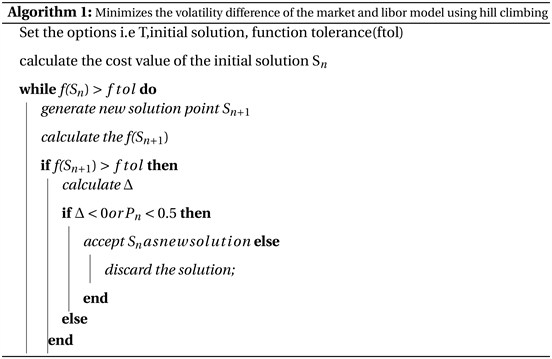
4.6. Simulated Annealing Minimization

Letting $\Omega$ be the discretized solution space and $f\mathrm{<mo>\; :\; </mo>}\Omega \to \Re$ , the objective function defined in the space. The algorithm searches the global minimum solution ${\omega }^g$ , such that $f\left({\omega }^g\right)<f\left(\omega \right)$ for all $\omega$ in $\Omega$ . The objective function is bounded for ${\omega }^g$ to exist. The objective function is used to calculate the cost value as;

${\left(\left|{\sigma }_i^{mkt}\left(t\right)-{\sigma }_i^{Lfr}\left(t\right)\right|\right)}^2\mathrm{.}$

4.6.1. Neighbourhood Function

In implementation, I will utilise the Boltz neighbourhood option to navigate the solution space. Boltz option uses a step length equal to the square root of temperature parameter to change from one solution to another with direction uniformly at random.

4.6.2. Cooling Schedule

There is no an academic consensus in regard to the choice of initial temperature. Most choices are made with regard to problem at hand. In implementation I use a default initial temperature of 100.

Afterwards the temperature is reduced by dividing the initial temperature with the logarithm of the rank of the iteration i.e.

$T_k=\frac{T_o}{\log k}\mathrm{,}$

k being the rank of the iteration.

4.6.3. Acceptance or Rejection Probability

Once a new solution has been sought, it’s compared to the previous solution, and accepted if better or the acceptance probability is between 0 and 0.5.

The acceptance function is:

$P_n=\frac{1}{1+{\exp }^{\frac{\Delta }{T_k}}}\mathrm{,}$

where:

· $\Delta$ is the difference between the current and previous cost value.

· T is the temperature parameter applicable at iteration k.

Stopping rule—The search stops when the set function tolerance is met.

4.7. Algorithm

4.8. Nonlinear Least-Squares (Lsqnonlin) Minimization

Least square is the oldest and most widely used minimisation method. Its popularity is due to the fact that it can be directly applied to a deterministic model without any cognizance being taken from the probability of the observations [25] . It is a constrained method that minimizes problems of the form;

$\underset{x}{\min }{\Vert f\left(x\right)\Vert }_2^2=\underset{x}{\min }\left(f_1{\left(x\right)}^2+f_2{\left(x\right)}^2+\cdots +f_n{\left(x\right)}^2\right)\mathrm{,}$

where the objective function ${\Vert f\left(x\right)\Vert }_2^2$ is defined in terms of auxiliary functions $f_i$ with optional lower and upper bounds on the components of x. The objective function corresponds to the residuals in a data fitting problem i.e.

$f\left(x\right)={\hat{y}}_i-y_i,$

where ${\hat{y}}_i$ is the model estimate and $y_i$ is the market observations.

Through an iteration procedure, the method minimises the sum of square residual value up to a set tolerance level. However, as against the Ordinary Least Squares (OLS) estimation, there is no closed-form solution for this system of equations formed, hence we make small adjustments to the predictor values at each iteration. Rather than computing the sum of least squares, the method requires a user-defined function to compute the vector-valued function $f_1\left(x\right)\mathrm{,}{f}_2\left(x\right)\mathrm{,}\cdots ,f_n\left(x\right)$ of the residuals.

4.9. Monte-Carlo Simulation

Monte-Carlo method is a numerical formula where random numbers are used for scientific experiment. Monte Carlo simulation is perchance the most common technique for propagating the incertitude of the various aspects of a system to the predicted performance. In Monte Carlo simulation, the entire system is simulated a large number of times i.e. a set of suitable sample paths is produced on $\left[t_0\mathrm{,}T\right]$ . Each simulation is equally likely and it’s referred to as a realization of the system. For each realization, all of the uncertain parameters are sampled. For each sample, we produce a sample path solution to the SDE on $\left[t_0\mathrm{,}T\right]$ . The realization is generally obtained from the stochastic Ito-Taylor expansion. From the Ito-Taylor expansion, we can construct numerical schemes for the interval $\left[t_i\mathrm{,}{t}_{i+1}\right]$ .

The dynamics of the libor rates under the Spot measure is:

$\text{d}{L}_k\left(t\right)={\sigma }_k\left(t\right)L_k\left(t\right){\displaystyle \underset{j=0+1}{\overset{\beta }{\sum }}}\frac{p_{k,j}{\tau }_j{\sigma }_j\left(t\right)L_j\left(t\right)}{1+{\tau }_j{L}_j\left(t\right)}\text{d}t+{\sigma }_k\left(t\right)L_k\left(t\right)\text{d}{Z}_k.$ (19)

Since the dynamics above doesn’t yield a distributionally known results, its proper to discretize it to finer time frame that would enable the process reduce the random inputs from distributionally known Gaussian shocks. Use of logarithm of the rates can help achieve the above objective. Taking logs and applying Ito’s lemma, dynamics of (19) become;

$\text{d}\ln L_k\left(t\right)={\sigma }_k\left(t\right){\displaystyle \underset{j=o+1}{\overset{\beta }{\sum }}}\frac{p_{k,j}{\tau }_j{\sigma }_j\left(t\right)L_j\left(t\right)}{1+{\tau }_j{L}_j\left(t\right)}\text{d}t-\frac{{\sigma }_k{\left(t\right)}^2}{2}\text{d}t+{\sigma }_k\left(t\right)\text{d}{Z}_k.$ (20)

Equation (20) has a diffusion process that is deterministic, as a consequence, the naive Euler scheme coincides with the more sophisticated Milstein scheme.

So the discretization becomes;

$\begin{array}{c}\ln L_k^{\Delta t}\left(t+\Delta t\right)=\ln L_k^{\Delta t}\left(t\right)+{\sigma }_k\left(t\right){\displaystyle \underset{j=o+1}{\overset{\beta }{\sum }}}\frac{p_{k,j}{\tau }_j{\sigma }_j\left(t\right)L_j^{\Delta t}\left(t\right)}{1+{\tau }_j{L}_j^{\Delta t}\left(t\right)}\Delta t\\ -\frac{{\sigma }_k{\left(t\right)}^2}{2}\Delta t+{\sigma }_k\left(t\right)\left(Z_k\left(t+\Delta t\right)-Z_k\left(t\right)\right).\end{array}$ (21)

This discretization leads to an approximation of the true process such that there exists a ${\gamma }_0$ with

$E^{\alpha }\left(\left|\ln L_k^{\Delta t}\left(t+\Delta t\right)-\ln L_k^{\Delta t}\left(t\right)\right|\right)\le C\left(T_o\right)\Delta t\mathrm{,}$

for $\Delta t\le {\gamma }_0$ , and $C\left(T_o\right)\Delta t$ is a positive constant. This gives strong convergence of order 1, from the exponent of $\Delta t$ on the right-hand side [3] .

For $k=o+1,o+2,\cdots ,\beta$ , we generate M of such realizations. After simulating the libor rates, they are subsequently used to calculate the swap rates through the relation indicated by section (4.3). Henceforth evaluating the payoff as:

${\displaystyle \underset{i=\alpha +1}{\overset{\beta }{\sum }}}P\left(T_o,T_i\right){\left(R_{0,\beta }-K\right)}^{+},$ (22)

for each realization and the average becomes the Swaption price.

Antithetic variates method for variance reduction was used to reduce the effects of discretization and simulation errors, so as to make sure that the price difference depicted is as a result of the different optimization techniques used.

4.10. Data

The data used in this study was obtained from [26] website. The data was used to price a swaption whilst using lsqnonlin method hence making it a good series to compare with simulated annealing performance.

5. Results & Discussion

In simulated annealing options, I used the Boltz method for my neighborhood and temperature function. For both SA and lsqnonlin, the feasible set of solutions had lower bound of [0 0 0.5 0 0.01] and upper bound of [1 1 2 0.3 1] with the initial point being [1.2.05 1.05.2]. The stopping criteria were based on the objective function achieving a tolerance of 1e−5.

5.1. Data Evaluation

The stylized features of the data can be ascribed from; the zero curves, forward curve and the evolution of the Libor market model rates. (Shown in Figure 2 below).

A zero curve maps the prices of zero coupon bonds to different maturities against time. This curve helps in pricing of fixed incomes securities and derivatives since it gives a fair value of capital gains accepted in the market. The slope of the curve indicates it is normal i.e. there is more compensation for each increment of risk taken. In derivatives market, longer time increases the chance of

negative events occurring hence higher risk.

Libor-forward rates can be transcribed from zero coupon bonds as shown in Equation (33) (in the appendix). They give insight to the price of a forward contract relative to its time to maturity. It is an experienced fact that the curve flattens out as time lapses. This because of increased correlation between the rates as time elapses.

The evolution of the market model is an indicator of the how the well the optimization techniques mimick the real world market. The two methods have managed to capture the sporadic movements of the libor rates, phenomena that become commonly observed after the financial crisis of 2007.

5.2. Volatility Function

The plots (Figure 3) below are the values of the stipulated volatility function whose parameters was estimated as [0.3744 0.0385 1.9454 0.1542] by SA method

and [0.0932 0.1524 0.5745 0.0707] by lsqnonlin method.

Market implied volatility curve is humped as a result of the control from the monetary authorities. The parameterization function adopted is capable of capturing the humped term structure of volatility in case the market volatility is originally humped. However, lsqnonlin looses the stylistic feature whereas SA is able to maintain it.

5.3. Correlation Matrices

As mentioned earlier, the terminal correlation of libor-forward rates do play a role in pricing swaption. The correlation is then used to calculate the value of the price. Below (Table 1) represent the correlation matrix that was calculated using the coefficient $\eta$ (0.0996) estimated by SA.

Lsqnonlin on the other hand, estimated the $\eta$ to be 0.0100, and corresponding correlation matrix is (Table 2).

The methods show typical qualities of a correlation matrix i.e. positive correlation with 1’s in the leading diagonal. Also moving away from the leading

diagonal, the measures are decreasing clearly showing that the joint movements of far away rates are less correlated than movements of rates with close maturities. The sub-diagonals are increasing as one approaches the leading diagonal, an indication of a larger correlation of adjacent rates.

Albeit the similarities, lsqnonlin predicts much higher correlations than SA. Such a flaw is undesired since the correlation is much lower for rates that are far off each other. SA doesn’t reflect the drawback.

5.4. Price Comparison

Table 3 below represents the prices of swaptions implied by the lsqnonlin method and the simulated annealing optimization, with their respective deviations from the Black’s prices. The swaption had a maturity of 5 years and a tenor ranging from 1 Year to 5 years. The instrument strike was 0.045.

The errors are plotted in the combined plot (Figure 4).

We set out to price a swaption using both lsqnonlin and simulated annealing optimization techniques, and did so by using the methods to minimize the difference between model volatility against market quotes. We have demonstrated that the simulated annealing produces lower errors than lsqnonlin as evident from the graph. Both methods value the swaption with a tenor of one as having an almost zero value hence same errors at onset. However as the swaption gains value, SA systematically predicts more precise prices than the contra.

6. Conclusions & Future Work

The goal of the thesis was to conduct a simulation test as to whether the SA optimization method outperforms the lsqnonlin method in finding a better solution to the volatility & correlation parametization functions when set under the same conditions. The methods were benchmarked against desirable market features.

The term structure of implied volatility is humped in nature indicating high uncertainty of intermediate forward rates. This phenomenon is a result of influence from the monetary authorities in that; at the short end of the maturity spectrum, the authorities determine the short deposit rates which then influence the short maturity forward rates, while at the long maturity spectrum, the authorities control the forward rates so as to achieve a set inflation target. This leaves the intermediate period as a time when loose or tight regimes can be reversed or continued beyond what was originally anticipated. This state of affairs gives rise to maximum market uncertainty in the intermediate-maturity region, hence the volatility of the long-dated or of the very-short-dated forward rates will not be as pronounced as that of the intermediate-maturity forward rates [27] . Albeit not identical to the market curve, volatility functions should be able to reflect the quantitative shape for proper derivative pricing. The results indicate that lsqnonlin misses portraying the hump of the intermediate rates instead showing only monotonic decaying volatility whereas SA features both the hump and the monotonic decay.

In a time-homogeneous world, decorrelation between two forward rates depends on how distant the rates are i.e. rates that are further apart are more decorrelated than the ones in close proximity. This is as a result of the shock affecting the first rate gradually dying out hence having little or no effect on the later rates. Although both techniques show this feature, in lsqnonlin method, it is less pronounced indicating that the rates are more correlated despite the dying off of the shock. On the other hand, SA adequately depicts this effect by having a more pronounced decorrelation among non-proximal rates.

The difference in the two methods to portray market features is easily depicted in the pricing of swaptions as evident from the value of errors and the graph. The more robust SA optimization has fewer errors propagated as compared to lsqnonlin, hence proving that indeed the lsqnonlin method does get trapped in the local minimum, consequently overstating the free parameters which in turn influence the price level.

The thesis thus proposes the adoption of simulated annealing optimization as the standard methodology for minimizing the difference between the model and market volatilities for greater price accuracy.

SA has many variant components including the use of linear decreasing temperature in lieu of lognormal, fast acceptance criterion instead of Boltz, and the maximum iteration stopping criteria as opposed to error tolerance. The thesis used the default options embedded in SA i.e. Boltz neighborhood function and decreasing lognormal temperature function, leaving the variants and custom functions for future study. The variants can be investigated to verify if they have less computational time than the ones used in the thesis.

The main drawback of the correlation function adopted is that it predicts the decorrelation of any two equidistant rates to be almost the same irrespective of whether the first forward rate expires in two months or one year i.e. the first and second rates will decorrelate just as much as the 9^th and the 10^th. Normally, long-dated rates are less decor-related than the short ones. This financially undesirable feature is a result of the absence of explicit time dependence in the function. A more desiderate specification would be the modified exponential form. Incorporation of the latter form and SA optimization could be investigated to discern if there is a further reduction in the disparity between numerical and analytical swaption prices.

Appendix

BGM Framework

BGM derivation begins from the Brace-Musiela (BM) (1994) parameterisation of the Heath-Jarrow-Morton (HJM) model. The HJM stochastic integration equation for under the the risk neutral measure is;

$f\left(t,T\right)=f\left(0,T\right)+{\displaystyle {\int }_0^t}a\left(\nu ,T\right)+{\displaystyle {\int }_0^t}\sigma \left(\nu ,T\right)\text{d}\hat{W}\left(\nu \right),$ (23)

where t is the time the rate is quoted and T is the time it applicable. Notably,T is fixed whereas t is a variable. For the model to be arbitrage free, the drift adopts the form,

$a\left(\nu \mathrm{,}T\right)=\sigma \left(t\mathrm{,}T\right){\displaystyle {\int }_t^T}\sigma \left(t\mathrm{,}s\right)\mathrm{.}$

BM considers a fixed period ahead rate

$\Upsilon \left(t\mathrm{,}x\right)\equiv f\left(t\mathrm{,}t+x\right)\mathrm{,}$ (24)

where $\Upsilon \left(t\mathrm{,}x\right)$ is the rate that is quoted at time t for instantaneous borrowing a time t + x, x being fixed time aheadi.e. 3 months. Hence Equation (23) becomes

$f\left(t\mathrm{,}t+x\right)=f\left(\mathrm{0,}t+x\right)+{\displaystyle {\int }_0^t}a\left(\nu \mathrm{,}t+x\right)+{\displaystyle {\int }_0^t}\sigma \left(\nu \mathrm{,}t+x\right)\text{d}\hat{W}\left(\nu \right)\mathrm{.}$ (25)

BM further redefines $\sigma \left(t\mathrm{,}t+x\right)$ as $\tau \left(t\mathrm{,}x\right)$ . With the above notation for drift and diffusion, the variables can written as

$\sigma \left(\upsilon ,t+x\right)=\sigma \left(\upsilon ,\upsilon +\left(t+x-\upsilon \right)\right)=\tau \left(\upsilon ,\left(t+x-\upsilon \right)\right),$

and

$a\left(\upsilon ,x\right)=a\left(\upsilon ,\upsilon +\left(t+x-\upsilon \right)\right)=a\left(\upsilon ,\left(t+x-\upsilon \right)\right).$

The notation will be of great importance when adopting the Heath-Jarrow-Morton drift restriction.

Adopting the BM notation, Equation (25) becomes;

$\Upsilon \left(t,x\right)=\Upsilon \left(0,t+x\right)+{\displaystyle {\int }_0^t}a\left(\upsilon ,\left(t+x-\upsilon \right)\right)\text{d}\upsilon +{\displaystyle {\int }_0^t}\tau \left(\upsilon ,\left(t+x-\upsilon \right)\right)\text{d}\hat{W}\left(\nu \right).$ (26)

In line with arbitrage free pricing, we adopt the notation of drift restriction as;

$\begin{array}{c}a\left(\nu ,t+x\right)=\sigma \left(t,t+x\right){\displaystyle {\int }_t^{t+x}}\sigma \left(t,s\right)\text{d}s\\ =\sigma \left(t,t+x\right){\displaystyle {\int }_0^x}\sigma \left(t,t+y\right)\text{d}s\\ =\tau \left(t,x\right){\displaystyle {\int }_0^x}\tau \left(t,y\right)\\ =\tau \left(t,x\right)\psi \left(t,x\right),\end{array}$

defining the integrated volatility as $\psi \left(t\mathrm{,}x\right)$ . The notation permits further manipulation of the drift as;

$a\left(\nu \mathrm{,}t+x\right)=\frac{\text{d}}{\text{d}x}\left(\frac{1}{2}{\psi }^2\left(t\mathrm{,}x\right)\right)\mathrm{,}$

and the diffusion as;

$\tau \left(t\mathrm{,}t+x\right)=\frac{\text{d}}{\text{d}x}\psi \left(t\mathrm{,}x\right)\mathrm{.}$

Not having t appearing in the second argument will be important in carrying out volatility transformations that will enable us have a log-normal libor rates.

Equation (26) is in stochastic integration form hence needs to transform to SDE by firstly differentiating with respect to x;

$\begin{array}{l}\frac{\text{d}}{\text{d}x}\Upsilon \left(t,x\right)={\Upsilon }_2\left(t,x\right)={\Upsilon }_2\left(0,t+x\right)+{\displaystyle {\int }_0^t}{a}_2\left(\upsilon ,\left(t+x-\upsilon \right)\right)\text{d}\upsilon \\ +{\displaystyle {\int }_0^t}{\tau }_2\left(\upsilon ,\left(t+x-\upsilon \right)\right)\text{d}\hat{W}\left(\nu \right).\end{array}$ (27)

And then forming the SDE as:

$\begin{array}{c}\text{d}\Upsilon \left(t,x\right)=[{\Upsilon }_2\left(0,t+x\right)+a\left(t,x\right)+{\displaystyle {\int }_0^t}{a}_2\left(\upsilon ,\left(t+x-\upsilon \right)\right)\text{d}\upsilon \\ +{\displaystyle {\int }_0^t}{\tau }_2\left(\upsilon ,\left(t+x-\upsilon \right)\right)\text{d}\hat{W}\left(\nu \right)]+\tau \left(t,x\right)\text{d}\hat{W}\left(\nu \right)\end{array}$ (28)

Adopting Equation (27)’s drift, and diffusion notation, the BGM Stochastic differential equation (SDE) for the instantaneous forward rate becomes

$\text{d}\Upsilon \left(t,x\right)=\frac{\text{d}}{\text{d}x}\left[\left(\Upsilon \left(t,x\right)+\frac{1}{2}{\psi }^2\left(t,x\right)\right)\text{d}t+\psi \left(t,x\right)\text{d}\hat{W}\left(t\right)\right].$

The above representation allows bond prices to be valued in terms of time to maturity i.e. the bond matures at a fixed period ahead in lieu of fixed date i.e.

$P\left(t\mathrm{,}T+x\right)=\exp \left[-{\displaystyle {\int }_t^T}r\left(t\mathrm{,}s-t\right)\text{d}s\right]\mathrm{,}$ (29)

where P (t, T + x) is the price of zero coupon bond at time t that will mature in x time period, x being some accrual period like 3 months.

By changing the variable $u=s-t$ , equation (29) becomes;

$P\left(t\mathrm{,}T\right)=\exp \left[-{\displaystyle {\int }_0^{T-t}}r\left(t\mathrm{,}u\right)\text{d}u\right]\mathrm{.}$ (30)

Libor

BGM instatenous forward rate relates to the libor process, $L\left(t,t+x+\delta \right)$ through the equation:

$1+\delta L\left(t\mathrm{,}t+x+\delta \right)=\exp \left[{\displaystyle {\int }_x^{x+\delta }}r\left(t\mathrm{,}x\right)\right]\mathrm{.}$ (31)

The libor is defined as a simple compounded rate that an investor can contract at time t for borrowing/lending over time $t+x$ to $t+x+\delta$ , $\delta$ being a discrete time tenor of maybe 3,6, or 12 months. Equation (31) also implies that the simple compounded rate must be in line with continuously compounded rate over the period.

In accordance with Equation (30), the rate can also relate to the bond prices as;

$1+\delta L\left(t,t+x+\delta \right)=\exp \left[{\displaystyle {\int }_x^{x+\delta }}r\left(t,x\right)\right]=\exp \left[{\displaystyle {\int }_0^{x+\delta }}r\left(t,x\right)-{\displaystyle {\int }_0^x}r\left(t,x\right)\right]$ (32)

$=\frac{P\left(t,T+x\right)}{P\left(t,T+x+\delta \right)}.$ (33)

To determine the SDE for Libor rate, we start by evaluate the quantity $\left[{\displaystyle {\int }_x^{x+\delta }}r\left(t\mathrm{,}x\right)\right]$ by equating to variable as;

$V\left(t\mathrm{,}x\right)={\displaystyle {\int }_x^{x+\delta }}r\left(t\mathrm{,}x\right)\mathrm{,}$ (34)

$\begin{array}{l}={\displaystyle {\int }_x^{x+\delta }}\Upsilon \left(0,t+x\right)\text{d}x+{\displaystyle {\int }_x^{x+\delta }}{\displaystyle {\int }_0^t}a\left(\upsilon ,\left(t+x-\upsilon \right)\right)\text{d}\upsilon \text{d}x\\ +{\displaystyle {\int }_x^{x+\delta }}{\displaystyle {\int }_0^t}\tau \left(\upsilon ,\left(t+x-\upsilon \right)\right)\text{d}\hat{W}\left(\nu \right)\text{d}x.\end{array}$ (35)

For a proper SDE, we need to change the order of integration using Fubini theorem, i.e.

$\begin{array}{l}={\displaystyle {\int }_x^{x+\delta }}\Upsilon \left(0,t+x\right)\text{d}x+{\displaystyle {\int }_0^t}{\displaystyle {\int }_x^{x+\delta }}a\left(\upsilon ,\left(t+x-\upsilon \right)\right)\text{d}x\text{d}\upsilon \\ +{\displaystyle {\int }_0^t}{\displaystyle {\int }_x^{x+\delta }}\tau \left(\upsilon ,\left(t+x-\upsilon \right)\right)\text{d}x\text{d}\hat{W}\left(\nu \right).\end{array}$ (36)

Differentiating Equation (36) with respect to t;

$\text{d}V=[{\displaystyle {\int }_x^{x+\delta }}{\Upsilon }_2\left(0,t+x\right)+{\displaystyle {\int }_0^t}{\displaystyle {\int }_x^{x+\delta }}{a}_2\left(\upsilon ,\left(t+x-\upsilon \right)\right)\text{d}x\text{d}\upsilon +{\displaystyle {\int }_x^{x+\delta }}a\left(t,\upsilon \right)\text{d}\upsilon$ (37)

$+{\displaystyle {\int }_0^t}{\displaystyle {\int }_x^{x+\delta }}{\tau }_2\left(\upsilon ,\left(t+x-\upsilon \right)\right)\text{d}x\text{d}\hat{W}\left(\nu \right)]\text{d}t+{\displaystyle {\int }_x^{x+\delta }}\tau \left(t,\upsilon \right)\text{d}\upsilon \hat{W}\left(\nu \right).$ (38)

From the above equation, the differentials can be simplified to;

$\begin{array}{c}{\displaystyle {\int }_x^{x+\delta }}{\Upsilon }_2\left(t,x\right)={\displaystyle {\int }_x^{x+\delta }}{\Upsilon }_2\left(0,t+x\right)+{\displaystyle {\int }_0^t}{\displaystyle {\int }_x^{x+\delta }}{a}_2\left(\upsilon ,\left(t+x-\upsilon \right)\right)\text{d}x\text{d}\upsilon \\ +{\displaystyle {\int }_0^t}{\displaystyle {\int }_x^{x+\delta }}{\tau }_2\left(\upsilon ,\left(t+x-\upsilon \right)\right)\text{d}x\text{d}\hat{W}\left(\nu \right),\end{array}$

$\begin{array}{c}\Upsilon \left(t,x+\delta \right)-\Upsilon \left(t,x\right)={\displaystyle {\int }_x^{x+\delta }}{\Upsilon }_2\left(0,t+x\right)+{\displaystyle {\int }_0^t}{\displaystyle {\int }_x^{x+\delta }}{a}_2\left(\upsilon ,\left(t+x-\upsilon \right)\right)\text{d}x\text{d}\upsilon \\ +{\displaystyle {\int }_0^t}{\displaystyle {\int }_x^{x+\delta }}{\tau }_2\left(\upsilon ,\left(t+x-\upsilon \right)\right)\text{d}x\text{d}\hat{W}\left(\nu \right),\end{array}$

hence Equation (38) can be rewritten as;

$\text{d}V=\left[\Upsilon \left(t,x+\delta \right)-\Upsilon \left(t,x\right)+{\displaystyle {\int }_x^{x+\delta }}a\left(t,\upsilon \right)\text{d}\upsilon \right]\text{d}t+{\displaystyle {\int }_x^{x+\delta }}\tau \left(t,\upsilon \right)\text{d}\upsilon \hat{W}\left(\nu \right).$ (39)

Adopting the notations;

${\displaystyle {\int }_x^{t+\delta }}a\left(t\mathrm{,}\upsilon \right)\text{d}u=\frac{1}{2}{\psi }^2\left(t\mathrm{,}x+\delta \right)-{\psi }^2\left(t\mathrm{,}x\right)\mathrm{,}$

${\displaystyle {\int }_x^{t+\delta }}\tau \left(t\mathrm{,}\upsilon \right)=\psi \left(t\mathrm{,}x+\delta \right)-\psi \left(t\mathrm{,}x\right)\mathrm{,}$

Equation (39) can be simplified further as;

$\text{d}V={\mu }_v\text{d}t+{\sigma }_v\text{d}{\hat{w}}_t\mathrm{,}$ (40)

where:

${\mu }_v=f\left(t,x+\delta \right)-f\left(t,x\right)+\frac{1}{2}{\psi }^2\left(t,x+\delta \right)-{\psi }^2\left(t,x\right),$ (41)

${\sigma }_v=\psi \left(t\mathrm{,}x+\delta \right)-\psi \left(t\mathrm{,}x\right)\mathrm{.}$ (42)

The quantity dV and application of Ito’s lemme can be used to derive the SDE of $L\left(t,t+x+\delta \right)$ (henceforth $L\left(t\mathrm{,}\delta \right)$ ) as;

$L\left(t\mathrm{,}\delta \right)=\frac{{\exp }^{V\left(t\mathrm{,}x\right)}-1}{\delta }\mathrm{,}$ (43)

$\text{d}L={\delta }^{-1}{\exp }^V\left({\mu }_v+\frac{1}{2}{\sigma }_v^2\right)+{\delta }^{-1}{\exp }^V{\sigma }_v\text{d}{\hat{W}}_t\mathrm{.}$ (44)

By observing that;

$\begin{array}{c}\frac{\text{d}}{\text{d}x}L\left(t\mathrm{,}\delta \right)={\delta }^{-1}\exp \left({\displaystyle {\int }_x^{x+\delta }}\Upsilon \left(t\mathrm{,}t+x\right)\right)\Upsilon \left(t\mathrm{,}t+x+\delta \right)-\Upsilon \left(t\mathrm{,}t+x\right)\mathrm{,}\\ ={\delta }^{-1}\left(1+\delta L\left(t\mathrm{,}\delta \right)\right)\Upsilon \left(t\mathrm{,}t+x+\delta \right)-\Upsilon \left(t\mathrm{,}t+x\right)\mathrm{,}\end{array}$

the SDE for $L\left(t\mathrm{,}\delta \right)$ can be expressed as;

$\begin{array}{c}\text{d}L\left(t,\delta \right)=\frac{\text{d}}{\text{d}x}L\left(t,\delta \right)+{\delta }^{-1}\left(1+\delta L\left(t,\delta \right)\right)\psi \left(t,x+\delta \right)\left(\psi \left(t,x+\delta \right)-\psi \left(t,x\right)\right)\text{d}t\\ +{\delta }^{-1}\left(1+\delta +L\left(t,\delta \right)\right)\left(\Upsilon \left(t,t+x+\delta \right)-\Upsilon \left(t,t+x\right)\right).\end{array}$ (45)

By further adopting the BGM volatility function

${\delta }^{-1}\left(1+\delta L\left(t\mathrm{,}\delta \right)\right)\psi \left(t\mathrm{,}x+\delta \right)-\psi \left(t\mathrm{,}x\right)=\gamma \left(t\mathrm{,}x\right)L\left(t\mathrm{,}\delta \right)\mathrm{,}$

where $\gamma \left(t\mathrm{,}x\right)$ is a function of time and maturity, Equation (45) can be rewritten as;

$\begin{array}{c}\text{d}L\left(t,\delta \right)=\left[\frac{\text{d}}{\text{d}x}L\left(t,\delta \right)+\gamma \left(t,x\right)L\left(t,\delta \right)\psi \left(t,x\right)+\frac{\delta {\gamma }^2\left(t,x\right)L^2\left(t,\delta \right)}{1+\delta L\left(t,\delta \right)}\right]\text{d}t\\ +\gamma \left(t,x\right)L\left(t,\delta \right)\text{d}\hat{W}\left(\upsilon \right).\end{array}$ (46)

Formulation (46) is the log-normal dynamics of the libor process that helps to recover the Black’s formula for Swaption prices, albeit it has a complicated drift term. BGM solution to the drift problem is considering another process $K\left(t,T\right)=L\left(t,T-t\right)$ . By taking differential with respect to the second argument,

$\text{d}K\left(t,T-t\right)=L\left(t,T-t\right)-L_2\left(t,T-t\right)\text{d}t,$ (47)

in deriving the equation above, BGM used the fact that that $L_2\left(t\mathrm{,}T-t\right)$ is smooth function of $L\left(t\mathrm{,}\delta \right)$ . A combinatorial of the BGM volatility function, Equation (45), and (47), the SDE for Libor process becomes

$\text{d}{L}_j=L_j\left(t\right){\gamma }_j\left(t\right)\left[{\psi }_{j+1}\left(t\right)\text{d}t+\text{d}\hat{W}\left(t\right)\right]$ (48)

Applying Girsanov theorem from risk -neutral measure to forward ( $T_{j+1}$ ) measure, changes BGM SDE to

$\text{d}{L}_j=L_j\left(t\right){\gamma }_j\left(t\right)\text{d}{W}^{T_{j+1}}\left(t\right)$ (49)

which is drift-less,( indicating it a martingale under the measure) and also posses the desirable property of being log-normal.

NOTES

¹Variables with the same value in all optimal solutions.

²Libor and BGM will be used interchangeably.

³e.g. under T-forward measure, the numeraire is a zero coupon bond whose price at maturity is a unit notional amount.

⁴Under risk neutral measure.

⁵The path-dependent derivatives can be accurately evaluated by constructing random paths of the libor process using either the forward-risk adjusted or spot Libor dynamics mainly because at each payment date $T_{j+1}$ spot Libor $L_j\left(t\right)$ is received and an amount equal τK is paid [23] .

Conflicts of Interest

The authors declare no conflicts of interest.

References

[1]	Barnes, C. (2021) Swaption Volumes by Strike Q1 2021. Clarus Financial Technology.
[2]	Fan, R., Gupta, A. and Ritchken, P. (2007) On Pricing and Hedging in the Swaption Market: How Many Factors, Really? The Journal of Derivatives, 15, 9-33. https://doi.org/10.3905/jod.2007.694699
[3]	Brigo, D. and Mercurio, F. (2007) Interest Rate Models-Theory and Practice: With Smile, Inflation and Credit. Springer Science & Business Media, Berlin.
[4]	Ledesma, S., Aviña, G. and Sanchez, R. (2008) Practical Considerations for Simulated Annealing Implementation. Simulated Annealing, 20, 401-420. https://doi.org/10.5772/5560
[5]	Ingber, L. (2000) Adaptive Simulated Annealing (ASA): Lessons Learned.
[6]	Rebonato, R. (1999) On the Simultaneous Calibration of Multifactor Lognormal Interest Rate Models to Black Volatilities and to the Correlation Matrix. Journal of Computational Finance, 2, 5-27. https://doi.org/10.21314/JCF.1999.031
[7]	Brace, A., Gatarek, D. and Musiela, M. (1997) The Market Model of Interest Rate Dynamics. Mathematical Finance, 7, 127-155. https://doi.org/10.1111/1467-9965.00028
[8]	Chiarella, C., He, X.Z., Nikitopoulos, C.S., et al. (2016) Derivative Security Pricing. Springer, Berlin. https://doi.org/10.1007/978-3-662-45906-5
[9]	Lagunzad, D.U. (2007) On the Calibration of the LIBOR Market Model. PhD Thesis, Singapore Management University, Singapore.
[10]	Jackel, P. and Rebonato, R. (2003) The Link between Caplet and Swaption Volatilities in a Brace-Gatarek-Musiela/Jamshidian Framework: Approximate Solutions and Empirical Evidence. Journal of Computational Finance, 6, 41-60. https://doi.org/10.21314/JCF.2003.100
[11]	Pascucci, A. and Riga, C. (2011) The Libor Market Model: From Theory to Calibration.
[12]	Ingber, L. (1989) Very Fast Simulated Re-Annealing. Mathematical and Computer Modelling, 12, 967-973. https://doi.org/10.1016/0895-7177(89)90202-1
[13]	Henderson, D., Jacobson, S.H. and Johnson, A.W. (2003) The Theory and Practice of Simulated Annealing. In: Handbook of Metaheuristics, Springer, Berlin, 287-319. https://doi.org/10.1007/0-306-48056-5_10
[14]	Kirkpatrick, S., Gelatt, C.D. and Vecchi, M.P. (1983) Optimization by Simulated Annealing. Science, 220, 671-680. https://doi.org/10.1126/science.220.4598.671
[15]	Martin, J.F.D. and Sierra, J.M.R. (2009) A Comparison of Cooling Schedules for Simulated Annealing (Artificial Intelligence). In: Encyclopedia of Artificial Intelligence, IGI Global, Hershey, 344-352. https://doi.org/10.4018/978-1-59904-849-9.ch053
[16]	Ben-Ameur, W. (2004) Computing the Initial Temperature of Simulated Annealing. Computational Optimization and Applications, 29, 369-385. https://doi.org/10.1023/B:COAP.0000044187.23143.bd
[17]	Gu, X. (2008) The Behavior of Simulated Annealing in Stochastic Optimization.
[18]	Luo, Y., Zhu, B. and Tang, Y. (2014) Simulated Annealing Algorithm for Optimal Capital Growth. Physica A: Statistical Mechanics and Its Applications, 408, 10-18. https://doi.org/10.1016/j.physa.2014.04.020
[19]	Fogarasi, N. and Levendovszky, J. (2013) Sparse, Mean Reverting Portfolio Selection Using Simulated Annealing. Algorithmic Finance, 2, 197-211. https://doi.org/10.3233/AF-13026
[20]	Beyna, I. and Wystup, U. (2010) On the Calibration of the Cheyette Interest Rate Model. Tech. Report, CPQF Working Paper Series.
[21]	Black, F. (1976) The Pricing of Commodity Contracts. Journal of Financial Economics, 3, 167-179. https://doi.org/10.1016/0304-405X(76)90024-6
[22]	Burgess, N. (2014) Martingale Measures & Change of Measure Explained. https://doi.org/10.2139/ssrn.2961006
[23]	Jamshidian, F. (1997) LIBOR and Swap Market Models and Measures. Finance and Stochastics, 1, 293-330. https://doi.org/10.1007/s007800050026
[24]	Rebonato, R., McKay, K. and White, R. (2009) The SABR/LIBOR Market Model: Pricing, Calibration and Hedging for Complex Interest-Rate Derivatives. John Wiley & Sons, Hoboken.
[25]	Bard, Y. (1974) Nonlinear Parameter Estimation. Tech. Rep.
[26]	Price Swaptions with Interest-Rate Models Using Simulation. https://uk.mathworks.com/help/fininst/price-bermudan-swaptions-with-different-interest-rate-models.html#bts_c9j-1
[27]	Rebonato, R. (2005) Volatility and Correlation: The Perfect Hedger and the Fox. John Wiley & Sons, Hoboken. https://doi.org/10.1002/9781118673539