1. Introduction
This article deals with the issue of disparity testing, i.e., testing the hypothesis that the mean of one group is larger than that of a second group when the groups from which samples are drawn are uncertain and given with a probability distribution. McDonald [1] presented relevant approaches and calculations for such testing, for both frequentist and Bayesian formulations, with two groups. In both formulations, use is made of all possible data configurations along with their corresponding probabilities for small sample sizes (≤6). Elkadry and McDonald [2] provide extensive discussion of the background giving rise to such disparity testing problems, and give an R-code to analyze sample sizes up to 22 using all possible data configurations. McDonald and Oakley [3] use a Bayesian framework and Markov Chain Monte Carlo sampling from the joint posterior distribution of the group means to estimate the probability of a disparity hypothesis. They provide the applicable R-codes and a WinBUGS code, and greatly extend sample size limitations of previous methods given in the literature. McDonald and Willard [4] , using a frequentist approach, employ a bootstrap methodology to generate summary statistics for the population of p-values arising from all possible configurations of the data to assess the credibility of the disparity hypothesis. Using their provided R-code, previous limitations on sample sizes are substantially eliminated. The p-value calculations for statistical hypotheses testing are presented in numerous texts (e.g., see Navidi [5] ).
The primary motivation for this work is the use of imputation of race/ethnicity of an individual based on available information such as surname and address. For example, in testing for disparity among race/ethnicity loan applicants where such information is not directly available, imputation methods are being used to assign one of six race/ethnicity groups to an application. There has been considerable research in developing such imputation methodology following the work of Fiscella and Fremont [6] . See, for example, the articles by Adjaye-Gbewonyo, et al. [7] , Brown, et al. [8] , Consumer Financial Protection Bureau [9] [10] , Elliott, et al. [11] , McDonald and Rojc [12] [13] [14] , Zhang [15] , and Zavez, et al. [16] for a wide variety of applications of such imputation methods in healthcare and finance using geocoding and surname analysis. Voicu, et al. [17] include the first name information, along with surname and geocoding, to improve the accuracy of race/ethnicity classification. To assess disparity of, say, auto loan rates extended to two race/ethnicity groups, a one-sided statistical hypothesis test could be used to assess the plausibility of the mean rate of one group being larger than that of another. This article addresses the issue of such statistical testing with imputed data as noted above.
This article expands the models used in references given above from two groups based on a binomial model to one using c groups (2 ≤ c ≤ 6) based on a mixture model within a Bayesian context. The methodologies developed in McDonald and Oakley [3] are applied with the more encompassing mixture likelihood function. Thus, this work is directly applicable to the output of proxy methods such as that from the Bayesian Improved Surname Geocoding (BISG) (see, e.g., Elliott, et al. [11] ) used extensively by the Consumer Financial Protection Bureau (CFPB) and others. Using BISG, the CFPB [9] ordered Ally Financial Inc. and Ally Bank to pay $80 million in damages to African-American, Hispanic, and Asian and Pacific Islander consumers harmed by Ally’s alleged discriminatory auto loan pricing, and $18 million in civil money penalties. The Wall Street Journal provides a website (published in 2015), http://graphics.wsj.com/ally-settlement-race-calculator/, implementing BISG for six race/ethnicity groups.
A Bayesian approach to the statistical hypothesis testing problem is utilized here. With this approach, the group means of the variable of interest (e.g., auto loan interest rates) are modeled with a probability distribution from which the probability of the disparity hypothesis can be calculated. Prior knowledge on the group means is combined with the likelihood function of the sample data to yield a so-called posterior probability distribution of the group means. Several approaches to these calculations are herein described and illustrated using computational codes given in the appendices. The illustrative calculations utilize one set of assumptions on the model and data (“noninformative” prior knowledge on the group means, and normal likelihood function for the sample data). However, the approach and computational tools given in the appendices are easily adapted to other assumptions. Hence the robustness of conclusions can be assessed with several other specifications of model assumptions. Some robustness considerations are explicitly considered in Sections 4 and 5.
Section 2 of this article describes the data set to be used subsequently to illustrate the computations of the various methodologies herein presented. It also applies a method labeled Laplace (Albert [18] ) to develop a multivariate normal distribution approximation to the posterior distribution of the group means. Section 3 details the use of “BayesMix”, an R-code, integrating several Metropolis-Hastings algorithms so as to generate draws from the posterior distribution of the group means. Using these draws, the mean values of the group means are calculated to assess the probabilities of linear contrasts of these mean values. The probability of a disparity hypothesis is calculated. Section 4 uses the publicly available software package WinBUGS to calculate quantities similar to those of Section 3. Gill [19] and Christensen, et al. [20] provide excellent introductions to Bayesian modeling emphasizing the use of both R and WinBUGS to analyze real data. Section 5 provides a summary and the concluding remarks.
2. Normal Approximation to the Posterior Distribution
2.1. The Data
To illustrate the following methodologies a simulated data set consisting of n = 18 observations, given in Appendix A, will be used. The data can be entered into the programs given in the Appendices B-D in several different manners, e.g., excel spreadsheet, list format, etc. The excel spreadsheet format will be used here with the R-code BayesMix given in Appendix B. The excel spreadsheet with the example data for this article is labeled “TestData.xlsx”. Two R packages are required for using this data format with the BayesMix: “readxl” and “LearnBayes”. The data of Appendix A were randomly drawn from a normal distribution in c = 6 groups of three—with means of 2, 4, 6, 8, 10, and 12, and with standard deviations of 1. The probabilities for the six categories of each datum are given as q = (q1, ···, q6). For each datum the category from which it was drawn is assigned the max probability. The objective of the analysis is to assess stochastic properties of the group means based on the data and group probabilities. These analyses will utilize algorithms given in Albert [18] and utilized in McDonald and Oakley [3] for c = 2. The user input required to execute BayesMix is given in Table 1. The specific values of the variables given in Appendix B used in this article are noted. The vector A, as given here, is used to formulate the disparity hypothesis “mu[2] is greater than mu[1]” for which its probability is estimated. Similarly, the contrast vector A1 is used for the hypothesis “mu[3] is greater than the average of mu[4] and mu[5]”. The quantities mu[i] refer to the group[i] means.
The output of BayesMix contains many data summaries and diagnostics useful in checking the analyses structures and calculations. The user can suppress one or more of these if so wished. However, the primary output is Table 2 (less the column WinBUGS).
2.2. Laplace
As described in the above references, the R-code Laplace computes the posterior mode of the vector mu = (mu[1], ···, mu[c]), the associated variance-covariance matrix, and an estimate of the logarithm of the normalizing constant for a general posterior density, and an indication of algorithm convergence (true or false). Three inputs are required: logpost, a function that defines the logarithm of the posterior density (denoted by loglike in Appendix B); mode, an initial guess at the posterior mode; par, a list of parameters associated with the function logpost.
The probability (posterior) density for the data is a mixture distribution given by
(1)
where 0 ≤ qi ≤ 1, ∑qi = 1, |x| < ∞, 0 < σ < ∞, and
is the normal probability density with mean and sigma equal to
evaluated at datum x.
![]()
Table 1. User required input for BayesMix (Appendix B).
![]()
Table 2. Output (to four dp) of BayesMix (Appendix B) and of WinBUGS (Appendix C) with Appendix A data.
The initial guess mode, a vector of length c, is denoted by mu in BayesMix. This initial guess can affect the convergence of the Laplace algorithm indicated by “true” or “false” in the output. One method for specifying this guess is to put each of the mu values equal to the average of the data. This has worked well for many of the calculations made in preparing this manuscript, but not all. There have been instances when the output of Laplace indicated “false” for convergence. In these cases, a good strategy is to rerun the Laplace function with the initial guess restated with the mode values output for the false convergence output. Another strategy that has worked very well, and is included in BayesMix, is to form the initial guess of mu[i] by taking the average of the data for which the category[i] has the maximum value over the c groups.
Laplace estimates of the mode values of the mu variables along with their standard deviations are given in Table 2 in the column denoted Lap. The estimates and standard deviations for mu[i] are denoted by esti and sdi, respectively. Since A is specified as (−1, 1, 0, 0, 0, 0), the vector (Ahi, Alo) = (2, 1) and the probability of mu[2] being greater than mu[1] is approximated with the normal distribution and the Laplace variance-covariance output as 0.9934. Also, A1 is specified by (0, 0, 1, −0.5, −0.5, 0), so Y = mu[3] − 0.5(mu[4] + mu[5]). Thus, Y > 0 is equivalent to mu[3] greater than the average of mu[4] and mu[5], the estimated probability of which is given in Table 2 as 0.0146. The entries in the other columns of Table 2, and the row “Accept Rate”, are explained in subsequent sections of this article.
While the Laplace algorithm with the normal approximation may not be most appropriate for the posterior distribution, the Laplace output provides very useful input to the algorithms to be utilized subsequently. The output of Laplace is explicitly used in the “proposal” and “start” inputs for the two Markov Chain Monte Carlo (MCMC) algorithms to be described in Section 3. BayesMix, which generated Table 2, ran in about 6.5 minutes on a laptop computer with Windows 10.
3. Exploring the Posterior Distribution with Metropolis-Hastings Algorithms
In this Section, random draws from the posterior distribution of the mean vector mu are used to estimate the probability of disparity as well as the cumulative probability distribution of any contrast of the category means. As was developed by McDonald and Oakley [3] , these draws are obtained using the popular MCMC methods in the Bayesian literature. As stated in Section 3 of the McDonald and Oakley reference, these methods consist of specifying an initial value for the parameter vector of interest and then generating a chain of values each of which depends only on the previous value in the chain. A rule for generating the sequence is a function of a proposal density and an acceptance probability. Not all generated values in the sequence are accepted as they must pass a probability criterion to be retained in the final sample. These components, the proposal density and acceptance probability criterion, are constructed so that the accepted simulated draws converge to draws from a random variable having the target posterior distribution. Different choices of the proposal density may result in slightly different distribution summaries.
Two such proposal density implementations described in detail by Albert [18] , and executed in the R package LearnBayes, are incorporated here in BayesMix given in Appendix B. The R functions “rwmetrop” and “indepmetrop” implement the so-called random walk and independence Metropolis-Hastings algorithms for special choices of the proposal densities. The methodology descriptions given in the following two subsections follow closely that of Section 3 of McDonald and Oakley [3] where the application is developed for c = 2 with a binomial likelihood. Here the applications are built for 2 ≤ c ≤ 6 with the likelihood function consisting of a mixture of normal densities given in Equation (1). The R-code BayesMix can be extended in a straightforward manner for c > 6, i.e., for more than six groups. However, the use of WinBUGS, described in Section 4, can be easily applied to cases of c > 6 by suitably stating the number of groups and appropriately entering the data in Appendix C and Appendix D.
Since the MCMC algorithms converge to sampling from the posterior distribution, initial draws may not be from the stationary distribution of the Markov chain, i.e., not drawn from the target posterior distribution. Thus, it is common practice to discard an initial portion of the draws and utilize the remainder. This practice is frequently referred to as “burn-in.” There are several diagnostics that can be viewed to help decide when the chain has progressed sufficiently far to stabilize on the posterior distribution (e.g., see Section 9.6 of Albert and Hu [21] ; Section 4.4.2 of Lunn et al. [22] ). Table 2 provides results based on 52,000 random draws using MCMC algorithms described in the following two subsections. Results are also provided following a burn-in of 2000 draws, i.e., results based on the last 50,000 random draws. As noted, the burn-in deletions result in very minor changes in the posted estimates for this illustrative data set. The two chains utilized in subsections 3.1 and 3.2 are described fully in Albert [18] .
3.1. Random Walk Metropolis Chain
Within LearnBayes, the function rwmetrop (logpost, proposal, start, m, par) requires five inputs: logpost, function defining the log posterior density; proposal, a list containing var, an estimated variance-covariance matrix, and scale, the Metropolis scale factor; start, a vector giving the starting value of the parameter; m, the number of iterations of the chain; par, the data used in the function logpost. The output is par, a matrix of the simulated values where each row corresponds to a value of the vector parameter; accept, the acceptance rate of the algorithm. A summary of the outputs of rwmetrop run with the specification of the data described in Section 2.1 with 52,000 draws from the posterior distribution is given in Table 2 in the column designated Ran.
As noted in the output, the acceptance rate here is 0.2191. The input “scale” should be chosen so that the acceptance rate is around 25%. Acceptance rates are discussed on page 121 of Albert [18] and on page 253 of Rizzo [23] . The acceptance rate is a decreasing function of scale.
The results following a burn-in of 2000 are given in Table 2 column RanRed. The results in this column are thus based on 50,000 draws and differ very little than those in column Ran.
3.2. Independence Metropolis Chain
The function indepmetrop (logpost, proposal, start, m, data) also requires five inputs: logpost, as above; proposal, a list containing mu, an estimated mean, and var, an estimated variance-covariance matrix for the normal proposal density; start, array with a single row that gives the starting value for the parameter vector; m, the number of iterations of the chain; data, data used in the function logpost. A summary of the outputs of indepmetrop run with the illustrative data set with 52,000 draws is given in Table 2 in the column designated Ind. Column IndRed provides analogous results for the 50,000 draws following the burn-in of 2000. As is the case with rwmetrop algorithm, there is negligible difference in the results with and without burn-in deletion.
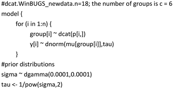
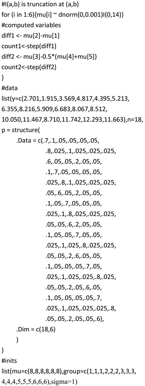
4. Applying WinBUGS for Bayesian Simulation
Another approach to generating draws from the posterior distribution is to use a MCMC software package, WinBUGS, designed specifically for Bayesian computation. WinBUGS is the MS Windows operating system version of BUGS, Bayesian Analysis Using Gibbs Sampling. There is a free download of this Bayesian software package available at the site (http://www.mrc-bsu.cam.ac.uk/bugs/overview/contents.shtml). Clear discussions of the applicability, limitations, and use of WinBUGS are given in Hahn [24] , Woodworth [25] , Lunn et al. [22] , and in many other references. The setup of this approach for the illustrative example considered here, where c = 6 and n = 18, is given in Appendix C. Note that in WinBUGS the normal distribution density is specified by dnorm(µ, τ), where µ is the mean and τ is the precision (= 1/variance). This differs from the specification in R, as given in Equation (1), where the normal distribution density at x is denoted by dnorm(x, µ, σ) with µ as the mean and σ as the standard deviation.
Output from WinBugs is given in Table 2 based on a sample of 50,000 draws from the posterior distribution following a burn-in of an initial 2000 draws (similar to that done for the RanRed and IndRed entries). A “count1” node is included to estimate P(mu[2] > mu[1]) as shown in Table 2. A similar “count2” node is included to estimate P(Y > 0) for a user specified transformation of the group means, A1 = (0, 0, 1, −0.5, −0.5, 0), in this example. To execute WinBugs, initial values are required for mu, group, and sigma. For mu, a reasonable choice for mu inits are the mode values given by Laplace. For group, a reasonable choice is to assign that group which has the largest probability for the datum. In case several groups share the largest value, choose one of those at random. For sigma, simply use a reasonable guess (e.g., use sigma = 1 as done here). The robustness of the results can easily be checked by running WinBUGS with other choices. The run time for WinBUGS as given in Appendix C is about forty seconds.
Appendix D provides a modification of the Appendix C WinBUGS program by treating sigma as an unknown value, common to all six groups, and to be estimated along with the other nodes. With this program, the mean of the 50,000 sigma draws is 0.9886 with a standard deviation of 0.3024. The output for the other nodes is very close to those given in Table 2 for WinBUGS with sigma fixed at one (i.e., the output using the Appendix C program). The P(m[2] > mu[1]) is estimated to be 0.9811, and P(Y > 0) to be 0.0689. A further extension of Appendix D can be made easily to accommodate the case where the group sigma values are not assumed known or to be equal.
5. Summary and Concluding Remarks
Table 2 shows a great deal of consistency with the entries, especially among the last five columns of the table. The results for the Laplace column also are in close agreement with those of the other columns, with perhaps the row entries corresponding to the standard deviations (i.e., sdi’s) where the Laplace values are uniformly a bit smaller than the others. The last five columns are based on statistics calculated from the random draws from the posterior distribution, whereas the Laplace column is based on a numerical fit to the data. These observations are based on the one data set given in Appendix A and may not generalize to other data sets. All the results given in this article apply to a mixture likelihood function of normal densities. Other densities could be substituted with appropriate changes in Equation (1) and appropriate modifications to the computer codes given in the Appendices.
An important question to be addressed with the methodologies used in this article is simply one of sample size. What is the tradeoff between the sample size (n) and the computing time? To partially address this issue, a sample of size n = 72 was constructed by pooling together four copies of the data given in Appendix A. The R-code in Appendix B and the WinBUGS code in Appendix C were run with exactly the same inputs used in Sections 3 and 4, with the expanded data set, generating an analogous Table 2. The laptop computer time for BayesMix was approximately forty-five minutes and for WinBUGS approximately forty seconds. The corresponding computer times with n = 18 (Appendix A) were approximately nine minutes for BayesMix and forty seconds for WinBUGS. There was no meaningful difference in computing times for WinBUGS between the two data sets. The output for the larger sample size closely matched that for the smaller sample size with the exception of the standard deviations (sdi’s) whose values with the larger data set were approximately half of the values with those obtained with the smaller set. For BayesMix, the computer time was approximately five times longer for n = 72 vs. n = 18. For much larger sample sizes, the bootstrap approach developed by McDonald and Willard [4] could be adapted to limit the required computing time.
As with all analyses, especially Bayesian, the robustness of the conclusions with respect to choices of model and prior specifications should be explored. With WinBUGS, a feature called “chains” facilitates running multiple MCMCs with different prior initializations given in the inits list. The priors used in this article were chosen to be so-called “noninformative” (e.g., distributions with very large variances). Other graphical diagnostics provided by WinBUGS are given in Appendix E for mu[1] and are very helpful in addressing the issue of stability of MCMC draws from a stationary posterior distribution. These diagnostics, along with similar ones for the other nodes, support the assessment that the MCMC draws are from a stable stationary posterior distribution. Chapter 6 of Hahn [24] and Chapter 14 of Gill [19] provide extensive discussion of assessing MCMC performance in WinBUGS along with some interfaces to R packages.
In conclusion, the Bayesian methods herein presented with appropriate computer codes provide a statistically sound basis for drawing conclusions about group disparity using race and ethnicity uncertainty data such as that arising with BISG and similarly based methodologies.
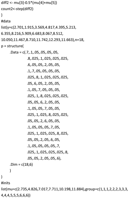
Appendix A. Excel Spreadsheet Data, TestData.xlsx
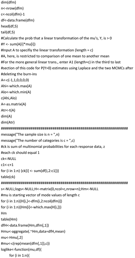
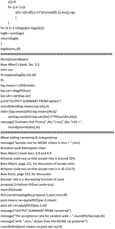
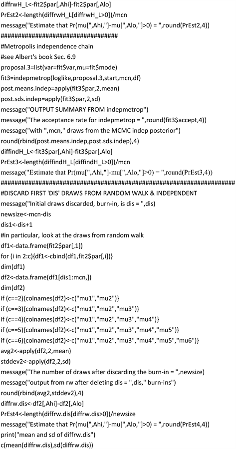
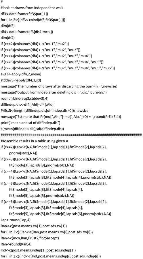
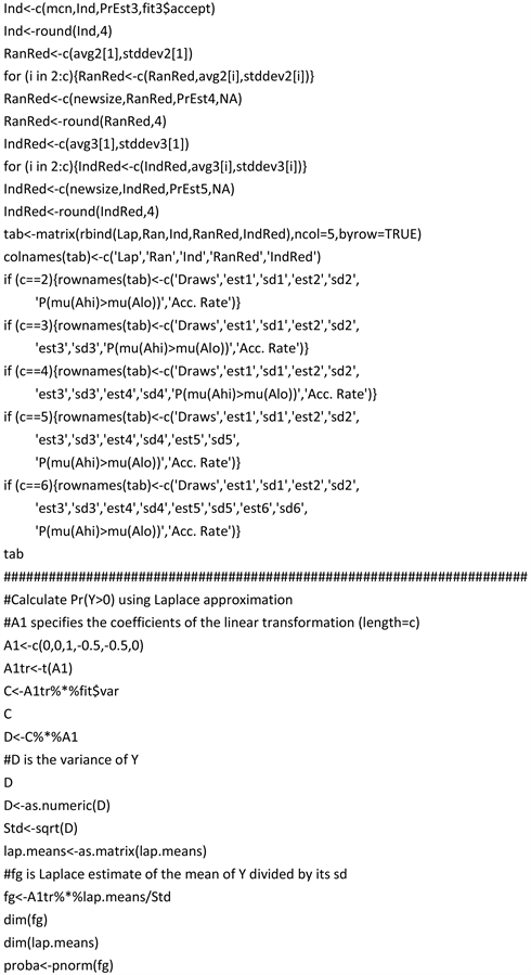
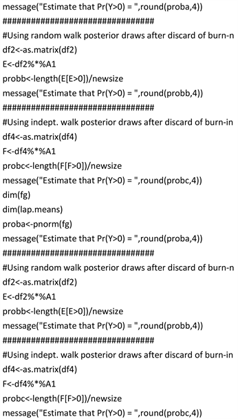
Appendix B. BayesMix Implementing Laplace, Metropolis-Hastings Algorithms

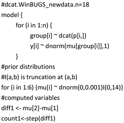
Appendix C. WinBUGS, Assuming σ = 1 for the c = 6 Groups
Appendix D. WinBUGS, Assuming a Common Unknown σ for the c = 6 Groups
Appendix E. WinBUGS Node Statistics Output and Graphical Diagnostics for mu[1] for Appendix 3 Run-From Top Left to Lower Right: Dynamic Trace, Running Quantiles, Time Series History, Kernel Density, and Autocorrelation Function