Abstract

In this research, we explore the properties and applications of the mapping cone and its variant, the pinched mapping cone. The mapping cone is a construction that arises naturally in algebraic topology and is used to study the homotopy type of spaces. It has several key properties, including its homotopy equivalence to the cofiber of a continuous map, and its ability to compute homotopy groups using the long exact sequence associated with the cofiber. We also provide an overview of the properties and applications of the mapping cone and the pinched mapping cone in algebraic topology. This work highlights the importance of these constructions in the study of homotopy theory and the calculation of homotopy groups. The study also points to the potential for further research in this area which includes the study of higher homotopy groups and the applications of these constructions to other areas of mathematics.

Keywords

Complex, Tensor Product, Pinched Tensor Product, Mapping Cone, Morphism

Share and Cite:

1. Introduction

The mapping cone is a construction used in algebraic topology and homological algebra to study maps between two topological spaces or algebraic objects. Let S, T, be two topological spaces and let $f\mathrm{<mo>\; :\; </mo>}S\to T$ be a continuous map from S to T. The mapping cone associated with f is a new space that captures information about the failure of f to be a homotopy equivalence.

Intuitively, the mapping cone is constructed by taking a cylinder $S\times \left[\mathrm{0,1}\right]$ and gluing one end to the image of S under f and the other end to a single point. The resulting space has a cone-like shape and encodes information about the twisting or winding of the map f.

In recent years, the mapping cone is used in algebraic topology to define the cone of a chain complex, which in turn is used to define the homology groups of a space. In homological algebra, the mapping cone is used to construct long exact sequences that relate the homology groups of two spaces connected by a map. Also it has been used for some discrete problems [1] and by bearing cone to estimate gazes in geological aspect of its applications [2] .

Algebraic topology was significantly advanced by the work of German mathematician Tammo tom Dieck [3] . His research had a profound impact on homotopy theory, particularly in stable homotopy theory and its applications. In [4] Dieck’s contributions encompassed work on the stable homotopy groups of spheres, surgery theory, and various other topics within algebraic topology. His research has greatly influenced the field, inspiring subsequent generations of mathematicians to explore these foundational ideas further.

Geometrically, the mapping cone of f can be visualized as the space obtained by gluing the cone over S to T via f. The chain complex $C\left(f\right)$ plays a pertinent role in algebraic topology, of note is its role in the study of spectral sequences and the long exact sequence of homology groups associated to a short exact sequence of chain complexes.

The pinched mapping cone of f has several important properties. First, it is homotopy equivalent to the suspension of the mapping cone $C\left(f\right)$ . This follows from the fact that the suspension of $C\left(f\right)$ is obtained by attaching two cones to its base, and the pinched mapping cone identifies the basepoints of these cones.

Second, the homotopy groups of the pinched mapping cone can be computed using the long exact sequence in homotopy associated with the mapping cone. This sequence relates the homotopy groups of S, T, and $C\left(f\right)$ , and can be used to compute the homotopy groups of Z.

Third, the pinched mapping cone is used in the proof of the Freudenthal suspension theorem, which relates the stable homotopy groups of spheres to the homotopy groups of suspensions of spheres. The pinched mapping cone is used to construct a sequence of maps that are used to show that the stable homotopy groups of spheres stabilize at a certain point.

For more details you may see in [5] [6] and [7] .

2. Basic Setup

It is assumed in this paper that E, F, S, and T are complexes of R-modules, with R being an associative ring. We will see most of the definitions and results of this section in [8] [9] and [10] .

Definition 2.1. A chain complex S of R-modules is a sequence of R-module homomorphisms,

$S\mathrm{<mo>\; :\; </mo>}\cdots \to S_{n+1}\stackrel{{\partial }_{n+1}^S}{\to }{S}_n\stackrel{{\partial }_n^S}{\to }{S}_{n-1}\to \cdots$

such that $Im{\partial }_{n+1}^S\subseteq \ker {\partial }_n^S$ for all n. Equivalently ${\partial }_n^S{\partial }_{n+1}^S=0$ , for all n. The maps ${\partial }_n$ are called the differentials of S.

Definition 2.2. Given a complex S of R-modules

$S\mathrm{<mo>\; :\; </mo>}\cdots \to S_{n+1}\stackrel{{\partial }_{n+1}^S}{\to }{S}_n\stackrel{{\partial }_n^S}{\to }{S}_{n-1}\to \cdots$

We say that it is exact at S_n if $Im{\partial }_{n+1}^S=\ker {\partial }_n^S$ . Moreover, we say S is an exact sequence if $Im{\partial }_{n+1}^S=\ker {\partial }_n^S$ for all n.

Definition 2.3. A morphism, or a degree zero chain map, $f\mathrm{<mo>\; :\; </mo>}S\to T$ between complexes S and T is a family of R-module homomorphisms $f_n$ , such that each square in the diagram

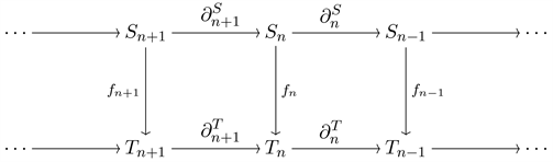
commutes. In other words, for each n we have $f_{n-1}{\partial }_n^S={\partial }_n^T{f}_n$ .

Also, if $f_n\mathrm{<mo>\; :\; </mo>}{S}_n\to T_n$ is an isomorphism for all n, then, S and T are said to be isomorphic, denoted by $\cong$ .

Definition 2.4. Let E be a complex of R-modules. Then the Shift of E, $\Sigma E$ is complex of R-modules defined by ${\left(\Sigma E\right)}_n=E_{n-1}$ , and ${\partial }_n^{\Sigma E}=-{\sigma }_{n-2}{\partial }_{n-1}^E{\sigma }_{n-1}^{-1}$ for all n. Also, the canonical map $\sigma \mathrm{<mo>\; :\; </mo>}E\to \Sigma E$ , is obtained by shifting degrees of elements, specifically, if $e\in E$ . Then, $\left|\sigma \left(e\right)\right|=\left|e\right|+1$ .

On the other hand, Lars Christensen and David Jorgensen unveiled in 2014 a variant of the tensor product of complexes in their paper [11] known as the pinched tensor product. We recall some essential definitions and recommendations.

Definition 2.5. Let S and T a complexes of R-modules. The tensor product $S{\otimes }_{R}T$ of S and T is specified by letting

${\left(S{\otimes }_{R}T\right)}_n={\displaystyle \underset{i\in \mathbb{Z}}{\coprod }{S}_i{\otimes }_R{T}_{n-i}}\mathrm{.}$

The differential is defined by,

${\partial }_n^{S{\otimes }_{R}T}\left(s\otimes t\right)={\partial }_i^S\left(s\right)\otimes t+{\left(-1\right)}^{i}s\otimes {\partial }_{n-i}^T\left(t\right)\mathrm{.}$

For $s\in S_i$ and $t\in T_{n-i}$ . The sign ${\left(-1\right)}^i$ ensures that ${\partial }_n^{S{\otimes }_{R}T}{\partial }_{n+1}^{S{\otimes }_{R}T}=0$ for all n.

Definition 2.6. Let S and T be complexes of R-modules. We define the pinched tensor product $S{\otimes }_R^{⊳⊲}T$ of S and T by:

${\left(S{\otimes }_R^{⊳⊲}T\right)}_n=(\begin{array}{ll}{\left(S_{\ge 0}{\otimes }_R{T}_{\ge 0}\right)}_n\hfill & \text{for}n\ge \text{0}\hfill \\ {\left(S_{\le -1}{\otimes }_R{\left(\Sigma T\right)}_{\le 0}\right)}_n\hfill & \text{for}n\le -\text{1}\text{.}\hfill \end{array}$

With differential ${\partial }^{S{\otimes }_R^{⊳⊲}T}$ defined by,

${\partial }_n^{S{\otimes }_R^{⊳⊲}T}=(\begin{array}{ll}{\partial }_n^{S_{\ge 0}{\otimes }_R{T}_{\ge 0}}\hfill & \text{for}n\ge \text{1}\hfill \\ {\partial }_0^S{\otimes }_R\left(\sigma {\partial }_0^T\right)\hfill & \text{for}n=\text{0}\hfill \\ {\partial }_n^{S_{\le -1}{\otimes }_R{\left(\Sigma T\right)}_{\le 0}}\hfill & \text{for}n\le -\text{1,}\hfill \end{array}$

where $\sigma$ denotes the canonical map $T\to \Sigma T$ .

For more details you may see [11] [12] and [13] .

3. Mapping Cone

Definition 3.1. Let A, B, S and T be complexes, and let $f\mathrm{<mo>\; :\; </mo>}S\to T$ and $g\mathrm{<mo>\; :\; </mo>}A\to B$ be chain maps. Then for $s\otimes a\in S_i\otimes A_{n-i}$ we have $\left(f\otimes g\right)\left(s\otimes a\right)={\left(-1\right)}^{\left|s\right|\left|g\right|}{f}_i\left(s\right)\otimes g_{n-i}\left(a\right)$ .

Definition 3.2. If $f\mathrm{<mo>\; :\; </mo>}S\to T$ is a chain map, then its mapping cone, $\text{cone}\left(f\right)$ , is a complex of R-modules whose term of degree n is $\text{cone}{\left(f\right)}_n={\left(\Sigma S\right)}_n\oplus T_n$ and whose differentials ${\partial }_n\mathrm{<mo>\; :\; </mo>}\text{cone}{\left(f\right)}_n\to \text{cone}{\left(f\right)}_{n-1}$ is given by

${\partial }_n^{\text{cone}\left(f\right)}=\left[\begin{array}{cc}{\partial }_n^{\Sigma S}& 0\\ f_{n-1}{\sigma }_{n-1}^{-1}& {\partial }_n^T\end{array}\right]\mathrm{.}$

A straightforward computation shows that ${\partial }_{n-1}^{\text{cone}\left(f\right)}{\partial }_n^{\text{cone}\left(f\right)}=0$ :

$\begin{array}{c}{\partial }_{n-1}^{\text{cone}\left(f\right)}{\partial }_n^{\text{cone}\left(f\right)}=\left[\begin{array}{cc}{\partial }_{n-1}^{\Sigma S}& 0\\ f_{n-2}{\sigma }_{n-2}^{-1}& {\partial }_{n-1}^T\end{array}\right]\left[\begin{array}{cc}{\partial }_n^{\Sigma S}& 0\\ f_{n-1}{\sigma }_{n-1}^{-1}& {\partial }_n^T\end{array}\right]\\ =\left[\begin{array}{cc}{\partial }_{n-1}^{\Sigma S}{\partial }_n^{\Sigma S}& 0\\ f_{n-2}{\sigma }_{n-2}^{-1}{\partial }_n^{\Sigma S}+{\partial }_{n-1}^T{f}_{n-1}{\sigma }_{n-1}^{-1}& {\partial }_{n-1}^T{\partial }_n^T\end{array}\right]=\left[\begin{array}{cc}0& 0\\ 0& 0\end{array}\right]\mathrm{.}\end{array}$

Since we know that f is a morphism and ${\partial }_n^{\Sigma S}=-{\sigma }_{n-2}{\partial }_{n-1}^S{\sigma }_{n-1}^{-1}$ .

Theorem 3.3. Let A be an R-complex and $f\mathrm{<mo>\; :\; </mo>}S\to T$ be a morphism of complexes of R-modules. Then,

$A{\otimes }_R\text{cone}\left(f\right)\cong \text{cone}\left(A{\otimes }_{R}f\right)\mathrm{.}$

Proof: The proof is well-known. (Proposition 4.1.12 in [14] .) □

4. Main Results

In the following section, we will present the main theorem applied in the special case of the pinched mapping cone and we provide the detailed proof of it.

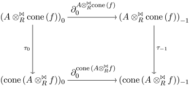
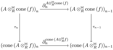
Theorem 4.1. Let A be an R-complex and $f\mathrm{<mo>\; :\; </mo>}S\to T$ be a morphism of complexes of R-modules. Then, there exist a morphism from $A{\otimes }_R^{⊳⊲}\text{cone}\left(f\right)$ to $\text{cone}\left(A{\otimes }_R^{⊳⊲}h\right)$ . Where, $h_n=f_n$ when $n\ge -1$ and $h_n=-f_n$ when $n<-1$

Proof: We consider three cases: $n=0$ , $n\ge 1$ and $n\le -1$ .

$n=0$ :

In this case the diagram is

Define ${\tau }_0\left(a\otimes \left(s\mathrm{,}t\right)\right)=\left({\sigma }_{-1}^{A{\otimes }_R^{⊳⊲}S}\left({\partial }_0^A\left(a\right)\otimes s\right)\mathrm{,}\left(a\otimes t\right)\right)$ and ${\tau }_{-1}\left(a\otimes {\sigma }_{-1}^{\text{cone}\left(f\right)}\left(s\mathrm{,}t\right)\right)=\left({\sigma }_{-2}^{A{\otimes }_R^{⊳⊲}S}\left(a\otimes t\right)\mathrm{,}\left(a\otimes {\sigma }_{-1}^T\left(t\right)\right)\right)$ . Choose an element $\left(a\otimes \left(s\mathrm{,}t\right)\right)\in A_0{\otimes }_R\left({\left(\Sigma S\right)}_0\oplus T_0\right)$ . Then,

$\begin{array}{l}{\partial }_0^{\text{cone}\left(A{\otimes }_R^{⊳⊲}f\right)}{\tau }_0\left(a\otimes \left(s\mathrm{,}t\right)\right)\\ ={\partial }_0^{\text{cone}\left(A{\otimes }_R^{⊳⊲}f\right)}\left({\sigma }_{-1}^{A{\otimes }_R^{⊳⊲}S}\left({\partial }_0^A\left(a\right)\otimes s\right)\mathrm{,}\left(a\otimes t\right)\right)\\ =[{\partial }_0^{\Sigma \left(A{\otimes }^{⊳⊲}S\right)}\left({\sigma }_{-1}^{A{\otimes }_R^{⊳⊲}S}\left({\partial }_0^A\left(a\right)\otimes s\right)\right)\mathrm{,}\\ \left(A_{-1}{\otimes }_R{\left(\Sigma f\right)}_0\right){\left({\sigma }_{-1}^{A{\otimes }_R^{⊳⊲}S}\right)}^{-1}{\sigma }_{-1}^{A{\otimes }_R^{⊳⊲}S}\left({\partial }_0^A\left(a\right)\otimes \left(s\right)\right)+{\partial }_0^{A{\otimes }^{⊳⊲}T}\left(a\otimes t\right)]\\ =[-{\sigma }_{-2}^{A{\otimes }_R^{⊳⊲}S}{\partial }_{-1}^{A{\otimes }^{⊳⊲}S}{\left({\sigma }_{-1}^{A{\otimes }_R^{⊳⊲}S}\right)}^{-1}\left({\sigma }_{-1}^{A{\otimes }_R^{⊳⊲}S}\left({\partial }_0^A\left(a\right)\otimes s\right)\right)\mathrm{,}\end{array}$

$\begin{array}{l}\stackrel{}{}\left(A_{-1}{\otimes }_R{\left(\Sigma f\right)}_0\right)\left({\partial }_0^A\left(a\right)\otimes \left(s\right)\right)+{\partial }_0^A\left(a\right)\otimes {\sigma }_{-1}^T{\partial }_0^T\left(t\right)]\\ =\left[-{\sigma }_{-2}^{A{\otimes }_R^{⊳⊲}S}{\partial }_{-1}^{A{\otimes }^{⊳⊲}S}\left({\partial }_0^A\left(a\right)\otimes s\right)\mathrm{,}\left({\partial }_0^A\left(a\right){\otimes }_R{\left(\Sigma f\right)}_0\left(s\right)\right)+{\partial }_0^A\left(a\right)\otimes {\sigma }_{-1}^T{\partial }_0^T\left(t\right)\right]\\ =[-{\sigma }_{-2}^{A{\otimes }_R^{⊳⊲}S}\left({\partial }_{-1}^A{\partial }_0^A\left(a\right)\otimes s+\left(-1\right){\partial }_0^A\left(a\right)\otimes {\partial }_{-1}^{\Sigma S}\left(s\right)\right)\mathrm{,}\\ \left({\partial }_0^A\left(a\right){\otimes }_R{\left(\Sigma f\right)}_0\left(s\right)\right)+{\partial }_0^A\left(a\right)\otimes {\sigma }_{-1}^T{\partial }_0^T\left(t\right)]\\ =\left[{\sigma }_{-2}^{A{\otimes }_R^{⊳⊲}S}\left({\partial }_0^A\left(a\right)\otimes {\partial }_{-1}^{\Sigma S}\left(s\right)\right)\mathrm{,}{\partial }_0^A\left(a\right){\otimes }_R{\left(\Sigma f\right)}_0\left(s\right)+{\partial }_0^A\left(a\right)\otimes {\sigma }_{-1}^T{\partial }_0^T\left(t\right)\right]\mathrm{.}\end{array}$

And

$\begin{array}{l}{\tau }_{-1}{\partial }_0^{A{\otimes }_R^{⊳⊲}\text{cone}\left(f\right)}\left(a\otimes \left(s\mathrm{,}t\right)\right)\\ ={\tau }_{-1}\left[{\partial }_0^A\left(a\right)\otimes {\partial }_0^{\text{Cone}\left(f\right)}\left(s\mathrm{,}t\right)\right]\\ ={\tau }_{-1}\left[{\partial }_0^A\left(a\right)\otimes \left({\partial }_{-1}^{\Sigma S}\left(s\right)\mathrm{,}{f}_{-1}{\left({\sigma }_{-1}^S\right)}^{-1}\left(s\right)+{\partial }_0^T\left(t\right)\right)\right]\\ =\left[{\sigma }_{-2}^{A{\otimes }_R^{⊳⊲}S}\left({\partial }_0^A\left(a\right)\otimes {\partial }_{-1}^{\Sigma S}\left(s\right)\right)\mathrm{,}{\partial }_0^A\left(a\right){\otimes }_R{\sigma }_{-1}^T\left(f_{-1}{\left({\sigma }_{-1}^S\right)}^{-1}\left(s\right)+{\partial }_0^T\left(t\right)\right)\right]\mathrm{.}\end{array}$

Clear that ${\left(\Sigma f\right)}_0\left(s\right)={\sigma }_{-1}^T{f}_{-1}{\left({\sigma }_{-1}^S\right)}^{-1}\left(s\right)$ since the following diagram commutes

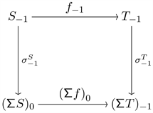
Therefore, ${\partial }_0^{\text{cone}\left(A{\otimes }_R^{⊳⊲}f\right)}{\tau }_0={\tau }_{-1}{\partial }_0^{A{\otimes }_R^{⊳⊲}\text{cone}\left(f\right)}$ , which is what we wanted to show.

$n\ge 1$ :

In this case the diagram is

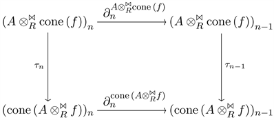
Define ${\tau }_n\left(a\otimes \left(s\mathrm{,}t\right)\right)=\left({\sigma }_{n-1}^{A{\otimes }_R^{⊳⊲}S}\left(a\otimes {\sigma }_i^{-1}\left(s\right)\right)\mathrm{,}\left(a\otimes t\right)\right)$ . We have two subcases $i=0$ and $i\ge 1$

$i=0$ :

Choose an element $\left(a\otimes \left(s\mathrm{,}t\right)\right)\in A_n{\otimes }_R\left({\left(\Sigma S\right)}_0\oplus T_0\right)$ . Then,

$\begin{array}{l}{\partial }_n^{\text{cone}\left(A{\otimes }_R^{⊳⊲}f\right)}{\tau }_n\left(a\otimes \left(s\mathrm{,}t\right)\right)\\ ={\partial }_n^{\text{cone}\left(A{\otimes }_R^{⊳⊲}f\right)}\left(\left(a\otimes t\right)\right)\\ =\left[{\partial }_n^{A{\otimes }^{⊳⊲}T}\left(a\otimes t\right)\right]\\ =\left[{\partial }_n^A\left(a\right)\otimes t+{\left(-1\right)}^{n}a\otimes {\partial }_0^T\left(t\right)\right]\mathrm{.}\end{array}$

And

$\begin{array}{l}{\tau }_{n-1}{\partial }_n^{A{\otimes }_R^{⊳⊲}\text{cone}\left(f\right)}\left(a\otimes \left(s\mathrm{,}t\right)\right)\\ ={\tau }_{n-1}\left[{\partial }_n^A\left(a\right)\otimes \left(s\mathrm{,}t\right)+{\left(-1\right)}^{n}a\otimes {\partial }_0^{\text{cone}\left(f\right)}\left(s\mathrm{,}t\right)\right]\\ ={\tau }_{n-1}\left[{\partial }_n^A\left(a\right)\otimes \left(s\mathrm{,}t\right)+{\left(-1\right)}^{n}a\otimes \left({\partial }_0^{\Sigma S}\left(s\right)\mathrm{,}{f}_{-1}{\left({\sigma }_{-1}^S\right)}^{-1}\left(s\right)+{\partial }_0^T\left(t\right)\right)\right]\\ =\left[{\partial }_n^A\left(a\right)\otimes t+{\left(-1\right)}^{n}a\otimes {\partial }_0^T\left(t\right)\right]\mathrm{.}\end{array}$

$i\ge 0$ :

Choose an element $\left(a\otimes \left(s\mathrm{,}t\right)\right)\in A_{n-i}{\otimes }_R\left({\left(\Sigma S\right)}_i\oplus T_i\right)$ . Then,

$\begin{array}{l}{\partial }_n^{\text{cone}\left(A{\otimes }_R^{⊳⊲}f\right)}{\tau }_n\left(a\otimes \left(s\mathrm{,}t\right)\right)\\ ={\partial }_n^{\text{cone}\left(A{\otimes }_R^{⊳⊲}f\right)}\left({\sigma }_{n-1}^{A{\otimes }_R^{⊳⊲}S}\left(a\otimes {\left({\sigma }_i^S\right)}^{-1}\left(s\right)\mathrm{,}\left(a\otimes t\right)\right)\right)\\ =[{\partial }_n^{\Sigma \left(A{\otimes }^{⊳⊲}S\right)}\left({\sigma }_{n-1}^{A{\otimes }_R^{⊳⊲}S}\left(a\otimes {\left({\sigma }_i^S\right)}^{-1}\left(s\right)\right)\right)\mathrm{,}\\ \left(A_{n-i}{\otimes }_R{f}_i\right){\left({\sigma }_{n-1}^{A{\otimes }_R^{⊳⊲}S}\right)}^{n-1}{\sigma }_{n-1}^{A{\otimes }_R^{⊳⊲}S}\left(a\otimes {\left({\sigma }_i^S\right)}^{-1}\left(s\right)\right)+{\partial }_n^{A{\otimes }^{⊳⊲}T}\left(a\otimes t\right)]\\ =[-{\sigma }_{n-2}^{A{\otimes }_R^{⊳⊲}S}{\partial }_{n-1}^{A{\otimes }^{⊳⊲}S}{\left({\sigma }_{n-1}^{A{\otimes }_R^{⊳⊲}S}\right)}^{-1}\left({\sigma }_{n-1}^{A{\otimes }_R^{⊳⊲}S}\left(a\otimes {\left({\sigma }_i^S\right)}^{-1}\left(s\right)\right)\right)\mathrm{,}\end{array}$

$\begin{array}{l}\left(A_{n-i}{\otimes }_R{f}_i\right)\left(a\otimes {\left({\sigma }_i^S\right)}^{-1}\left(s\right)\right)+{\partial }_{n-i}^A\left(a\right)\otimes t+{\left(-1\right)}^{n-i}a\otimes {\partial }_i^T\left(t\right)]\\ =[-{\sigma }_{n-2}^{A{\otimes }_R^{⊳⊲}S}{\partial }_{n-1}^{A{\otimes }^{⊳⊲}S}\left(a\otimes {\left({\sigma }_i^S\right)}^{-1}\left(s\right)\right)\mathrm{,}\\ \left(a{\otimes }_R{f}_i{\left({\sigma }_i^S\right)}^{-1}\left(s\right)\right)+{\partial }_{n-i}^A\left(a\right)\otimes t+{\left(-1\right)}^{n-i}a\otimes {\partial }_i^T\left(t\right)]\\ =[-{\sigma }_{n-2}^{A{\otimes }_R^{⊳⊲}S}\left({\partial }_{n-i}^A\left(a\right)\otimes {\left({\sigma }_i^S\right)}^{-1}\left(s\right)+{\left(-1\right)}^{n-i}a\otimes {\partial }_{i-1}^S{\left({\sigma }_{i-1}^S\right)}^{-1}\left(s\right)\right)\mathrm{,}\\ \left(a{\otimes }_R{f}_i{\left({\sigma }_i^S\right)}^{-1}\left(s\right)\right)+{\partial }_{n-i}^A\left(a\right)\otimes t+{\left(-1\right)}^{n-i}a\otimes {\partial }_i^T\left(t\right)]\mathrm{.}\end{array}$

And

$\begin{array}{l}{\tau }_{n-1}{\partial }_n^{A{\otimes }_R^{⊳⊲}\text{cone}\left(f\right)}\left(a\otimes \left(s\mathrm{,}t\right)\right)\\ ={\tau }_{n-1}\left[{\partial }_{n-i}^A\left(a\right)\otimes \left(s\mathrm{,}t\right)+{\left(-1\right)}^{n-i}a\otimes {\partial }_i^{\text{cone}\left(f\right)}\left(s\mathrm{,}t\right)\right]\end{array}$

$\begin{array}{l}={\tau }_{n-1}\left[{\partial }_{n-i}^A\left(a\right)\otimes \left(s\mathrm{,}t\right)+{\left(-1\right)}^{n-i}a\otimes \left({\partial }_i^{\Sigma S}\left(s\right)\mathrm{,}{f}_{i-1}{\left({\sigma }_{i-1}^S\right)}^{-1}\left(s\right)+{\partial }_i^T\left(t\right)\right)\right]\\ =[-{\sigma }_{n-2}^{A{\otimes }_R^{⊳⊲}S}\left({\partial }_{n-i}^A\left(a\right)\otimes {\left({\sigma }_i^S\right)}^{-1}\left(s\right)+{\left(-1\right)}^{n-i}a\otimes {\left({\sigma }_{i-1}^S\right)}^{-1}{\partial }_i^{\Sigma S}\left(s\right)\right)\mathrm{,}\\ a\otimes f_{i-1}{\left({\sigma }_{i-1}^S\right)}^{-1}\left(s\right)+{\partial }_{n-i}^A\left(a\right)\otimes t+{\left(-1\right)}^{n-i}a\otimes {\partial }_i^T\left(t\right)]\mathrm{.}\end{array}$

Therefore, ${\partial }_n^{\text{cone}\left(A{\otimes }_R^{⊳⊲}f\right)}{\tau }_n={\tau }_{n-1}{\partial }_n^{A{\otimes }_R^{⊳⊲}\text{cone}\left(f\right)}$ , which is what we wanted to show.

$n\le -1$ :

In this case the diagram is

Define ${\tau }_n\left(a\otimes {\sigma }_n^{\text{cone}\left(f\right)}\left(s\mathrm{,}t\right)\right)=\left({\sigma }_{n-1}^{A{\otimes }_R^{⊳⊲}S}\left(a\otimes {\sigma }_i^{-1}\left(s\right)\right)\mathrm{,}\left(a\otimes {\sigma }_i^T\left(t\right)\right)\right)$ and choose an element $\left(a\otimes \left(s\mathrm{,}t\right)\right)\in A_i{\otimes }_R\left({\left(\Sigma S\right)}_{n-i-1}\oplus T_{n-i-1}\right)$ . Then,

$\begin{array}{l}{\partial }_n^{\text{cone}\left(A{\otimes }_R^{⊳⊲}f\right)}{\tau }_n\left(a\otimes {\sigma }_n^{\text{cone}\left(f\right)}\left(s\mathrm{,}t\right)\right)\\ ={\partial }_n^{\text{cone}\left(A{\otimes }_R^{⊳⊲}f\right)}\left({\sigma }_{n-1}^{A{\otimes }_R^{⊳⊲}S}\left(a\otimes {\sigma }_i^{-1}\left(s\right)\right)\mathrm{,}\left(a\otimes {\sigma }_i^T\left(t\right)\right)\right)\\ =[{\partial }_n^{\Sigma \left(A{\otimes }^{⊳⊲}S\right)}\left({\sigma }_{n-1}^{A{\otimes }_R^{⊳⊲}S}\left(a\otimes s\right)\right)\mathrm{,}\left(A_i{\otimes }_R{\left(\Sigma f\right)}_{n-1-i}\right){\left({\sigma }_{n-1}^{A{\otimes }_R^{⊳⊲}S}\right)}^{n-1}{\sigma }_{n-1}^{A{\otimes }_R^{⊳⊲}S}\left(a\otimes s\right)\\ \stackrel{}{}+{\partial }_n^{A{\otimes }^{⊳⊲}T}\left(a\otimes {\sigma }_i^T\left(t\right)\right)]\\ =[-{\sigma }_{n-2}^{A{\otimes }_R^{⊳⊲}S}{\partial }_{n-1}^{A{\otimes }^{⊳⊲}S}{\left({\sigma }_{n-1}^{A{\otimes }_R^{⊳⊲}S}\right)}^{n-1}\left({\sigma }_{n-1}^{A{\otimes }_R^{⊳⊲}S}\left(a\otimes s\right)\right)\mathrm{,}\left(A_i{\otimes }_R{\left(\Sigma f\right)}_{n-1-i}\right)\left(a\otimes s\right)\end{array}$

$\begin{array}{l}\stackrel{}{}+{\partial }_i^A\left(a\right)\otimes {\sigma }_i^T\left(t\right)+{\left(-1\right)}^{i}a\otimes {\partial }_{n-i}^{\Sigma T}{\sigma }_i^T\left(t\right)]\\ =[-{\sigma }_{n-2}^{A{\otimes }_R^{⊳⊲}S}{\partial }_{n-1}^{A{\otimes }^{⊳⊲}S}\left(a\otimes s\right)\mathrm{,}\left(a{\otimes }_R{\left(\Sigma f\right)}_{n-1-i}\left(s\right)\right)\\ +{\partial }_i^A\left(a\right)\otimes {\sigma }_i^T\left(t\right)+{\left(-1\right)}^{i}a\otimes {\partial }_{n-i}^{\Sigma S}{\sigma }_i^T\left(t\right)]\\ =[-{\sigma }_{n-2}^{A{\otimes }_R^{⊳⊲}S}\left({\partial }_i^A\left(a\right)\otimes s+{\left(-1\right)}^{i}a\otimes {\partial }_{n-i-1}^{\Sigma S}\left(s\right)\right)\mathrm{,}\left(a{\otimes }_R{\left(\Sigma f\right)}_{n-1-i}\left(s\right)\right)\\ +{\partial }_i^A\left(a\right)\otimes {\sigma }_i^T\left(t\right)+{\left(-1\right)}^{i}a\otimes {\partial }_{n-i}^{\Sigma T}{\sigma }_i^T\left(t\right)]\mathrm{.}\end{array}$

And

$\begin{array}{l}{\tau }_{n-1}{\partial }_n^{A{\otimes }_R^{⊳⊲}\text{cone}\left(f\right)}\left(a\otimes \left(s\mathrm{,}t\right)\right)\\ ={\tau }_{n-1}\left[{\partial }_i^A\left(a\right)\otimes \left(s\mathrm{,}t\right)+{\left(-1\right)}^{i}a\otimes {\partial }_{n-i}^{\text{cone}\left(f\right)}\left(s\mathrm{,}t\right)\right]\\ ={\tau }_{n-1}\left[{\partial }_i^A\left(a\right)\otimes \left(s\mathrm{,}t\right)+{\left(-1\right)}^{i}a\otimes \left({\partial }_{n-i}^{\Sigma S}\left(s\right)\mathrm{,}{\left(\Sigma f\right)}_{n-i-1}{\left({\sigma }_{n-i-1}^S\right)}^{-1}\left(s\right)+{\partial }_{n-i}^T\left(t\right)\right)\right]\\ =[-{\sigma }_{n-2}^{A{\otimes }_R^{⊳⊲}S}\left({\partial }_i^A\left(a\right)\otimes s+{\left(-1\right)}^{i}a\otimes {\partial }_{n-i}^{\Sigma S}\left(s\right)\right)\mathrm{,}{\left(-1\right)}^{i}a\otimes {\left(\Sigma f\right)}_{n-i}{\left({\sigma }_{n-i}^S\right)}^{-1}\left(s\right)\\ +{\partial }_i^A\left(a\right)\otimes {\sigma }_i^T\left(t\right)+{\sigma }_{n-i-1}^T{\partial }_{n-i}^T\left(t\right)]\mathrm{.}\end{array}$

Therefore, ${\partial }_n^{\text{cone}\left(A{\otimes }_R^{⊳⊲}f\right)}{\tau }_n={\tau }_{n-1}{\partial }_n^{A{\otimes }_R^{⊳⊲}\text{cone}\left(f\right)}$ , which is what we wanted to show. □

Remark 4.2. In Theorem 4.1 we note that we will not have an isomorphism between $A{\otimes }_R^{⊳⊲}\text{cone}\left(f\right)$ and $\text{cone}\left(A{\otimes }_R^{⊳⊲}f\right)$ because ${\left(C{\otimes }_R^{⊳⊲}\text{cone}\left(f\right)\right)}_n$ has one more term than ${\left(\text{cone}\left(A{\otimes }_R^{⊳⊲}f\right)\right)}_n$ for $n>0$ and vice versa for $n<0$ .

Theorem 4.3. Let A be an R-complex and $f\mathrm{<mo>\; :\; </mo>}S\to T$ be a morphism of complexes of R-modules. Then there exist a morphism from $\text{cone}\left(A{\otimes }_R^{⊳⊲}f\right)$ to $A{\otimes }_R^{⊳⊲}\text{cone}\left(f\right)$ .

Proof: The proof is similar to that of Theorem 4.1. □

5. Conclusion

To conclude, the mapping cone stands as a potent instrument within algebraic topology, boasting myriad vital applications. Its inherent properties facilitate the establishment of intriguing connections among homotopy groups of spaces, playing a pivotal role in substantiating numerous key theorems. The mapping cone’s versatility extends its utility across a wide array of subjects, spanning from homotopy groups to fiber bundles. For algebraic topologists, it remains an indispensable tool, frequently employed to tackle the challenging computation of homotopy groups. Notably, the pinched mapping cone serves as a testament to the robustness and value of algebraic topology in the realm of mathematics. As referenced in the central theorem, we substantiate the existence of morphisms from one cone to another, contributing significantly to the expansion of homotopy group properties. Future research avenues may delve even deeper into the intricacies of the mapping cone, providing more extensive exploration of its applications and investigating its pertinence in other mathematical domains.

Acknowledgements

It is our pleasure to acknowledge profitable discussions with Professor Dr. David A. Jorgensen. We would also like to appreciate the referees for their helpful comments and improvements. Also, we wish to acknowledge the generous financial support from the Public Authority for Applied Education and Training for supporting this research, project No. BE-21-05.

Conflicts of Interest

The author declares no conflicts of interest regarding the publication of this paper.

References