
The Vertical Force Estimation Algorithm Based on Smart Tire Technology
by
 , ,
, ,
Tianli Gu
1 ,
,
Bo Li
1,2,*,
Zhenqiang Quan
1,
Shaoyi Bei
1,*,
Guodong Yin
3,
Jinfei Guo
1,
Xinye Zhou
1 and
Xiao Han
2 1
School of Automotive and Transportation Engineering, Jiangsu University of Technology, Changzhou 213000, China
2
Suzhou Automotive Research Institute, Tsinghua University, Suzhou 215200, China
3
School of Mechanical Engineering, Southeast University, Nanjing 211189, China
*
Authors to whom correspondence should be addressed.
World Electr. Veh. J. 2022, 13(6), 104; https://doi.org/10.3390/wevj13060104
Submission received: 14 May 2022
/
Revised: 4 June 2022
/
Accepted: 9 June 2022
/
Published: 13 June 2022
(This article belongs to the Special Issue Trends and Emerging Technologies in Electric Vehicles)
Abstract
:The real-time monitoring of the vertical force of the tire is the basis for ensuring the driving safety, handling stability, fuel economy and the riding comfort of the vehicle. An algorithm for the vertical force of the tire estimation based on the combination of intelligent tire technology and neural network theory is herein proposed. Firstly, the finite element model of the 205/55/R16 radial tire was established by ABAQUS and the validity of the finite element model was verified through static experiment and dynamic experiment. Secondly, the effects of inflation pressure, speed, load and tread wear on the tire contact patch length and the radial displacement at the virtual acceleration sensor were analyzed based on the finite element analysis method and control variable method. Finally, three kinds of the vertical force prediction algorithms based on the GA-BP neural network algorithm were established, and the network performance of each prediction model was tested. The results show that the vertical force prediction model with inflation pressure and the peak value of radial displacement as the characteristic input parameters has the highest prediction accuracy and the shortest calculation time. At the same time, the mathematical formula of the Model 3 was built.
1. Introduction
The contact between the tire and the road surface is the main source of tire force, and the online estimation of tire force is the basis for ensuring the driving safety, handling stability, fuel economy and the riding comfort of the car [1]. Tire vertical force is one of the necessary input parameters of the vehicle chassis safety control system, and it is also an important factor affecting the tire lateral force and longitudinal force [2]. Therefore, it is crucial to design a method that can monitor the vertical force of tires online.
Scholars at home and abroad have carried out much research on tire vertical force prediction. Most of the traditional tire vertical force prediction research is related to the construction of the vehicle dynamics model, tire model or observer, such as the Dugoff model [3] and the Pacejka semi-empirical tire model [4], etc. It is worth noting that some of the parameters contained in these tire models need to be calibrated from time to time through tire characteristic tests, because these parameters change as the tire ages, causing the tire model to be inaccurate. Cho et al. [5] analyzed the law of vehicle static load and longitudinal and lateral load transfer and reconstructed the expression form of tire vertical force combined with tire model. Doumiati et al. [6] proposed a tire vertical force model based on the coupling of longitudinal load transfer and lateral load transfer and combined the random walk Kalman filter to estimate the tire vertical force. Ye et al. [7] predicted the vertical force of the tire based on the real vehicle data collected by the on-board sensors, combined with the seven-degree-of-freedom vehicle model and the RKF algorithm. Antonov et al. [8] proposed a tire vertical force prediction method based on suspension, wheel and stabilizer offset signals. The traditional vertical force prediction method has two obvious shortcomings: (1) The complexity of the vehicle model or tire model is irreconcilable with the accuracy of the prediction results; (2) there are certain errors and uncertainties in the prediction of the tire force based on the signals collected by on-board sensors.
Therefore, scholars in the field of automobiles or tires have proposed a vertical force prediction method based on the combination of smart tire technology that tire information directly monitored by sensors installed inside the tire and machine learning theory [9]. Compared with the traditional vertical force prediction method, this type of vertical force prediction method has two significant advantages: (1) the tire-sensor directly collects tire dynamic information, reducing the error of on-board sensors signal collection, and (2) the relationship between characteristic parameters and tire vertical force is directly established through the machine learning theory, which reduces the computational complexity of vertical force prediction. Garcia-Pozuelo et al. [10] propose novel algorithm based on fuzzy logic to estimate the mentioned parameters by means of a single strain-based system. Huang et al. [11] used the signals collected by MEMS acceleration, inflation pressure and temperature sensors as the reference signal and extracted the eigenvalues to build a tire vertical force prediction algorithm. Zhao et al. [12] built a real vehicle test platform for intelligent tires based on embedded accelerometers, extracted typical characteristics of acceleration signals and a combined BP neural network algorithm to predict the vertical force of tires. Xu et al. [13] built a smart tire signal acquisition system based on a three-axis accelerometer and collected the eigenvalues of acceleration signals under various working conditions through tire characteristic experiments. Finally, they built a prediction of tire vertical force method based on machine learning algorithms. At present, the vertical force estimation method based on the smart tire technology is usually obtained by using the relationship between the vertical force and the longitudinal contact patch length, wherein the longitudinal contact length is obtained indirectly through the acceleration signal. However, there are many factors that affect the longitudinal contact patch length, which can lead to the high computational complexity of the prediction algorithm. Moreover, the current data collection conditions of the vertical force prediction algorithm only consider the inflation pressure, load and vehicle speed, ignoring the influence of the tire wear on the length of the longitudinal contact patch length. Therefore, this paper aims to explore one or more characteristic parameters that are highly correlated with vertical force, are more stable and not affected by tire wear and use this to build a robust and low-computational vertical force estimation algorithm. There are many types of sensors currently used in the field of intelligent tires, including strain sensors [14], optical sensors [15], magnetic sensors [16], piezoelectric sensors [17], surface acoustic wave sensors [18], acceleration sensors [19] and so on. By comparing the advantages and disadvantages of the above different sensors, this paper chooses the triaxial accelerometer as the sensor of the intelligent tire system, the main reason is that the acceleration signal is closely related to the tire force, and the triaxial accelerometer also has the advantages of small size and light weight.
Firstly, the finite element model of the 205/55R16 radial tire was established by using ABAQUS software, and the validity of the finite element model was verified through the static experiment and dynamic experiment. Secondly, the effects of inflation pressure, load, speed and tread wear on the tire contact patch and the radial displacement at the position of the virtual acceleration sensor were analyzed based on the finite element analysis method and the control variable method. Finally, according to the difference in the selection of input feature parameters, the paper built three vertical force estimation models based on the GA-BP neural network algorithm and compared and analyzed the mean absolute error, mean absolute percentage error and forecast computation time.
2. Establishment of the Tire Finite Element Model
2.1. Element Type
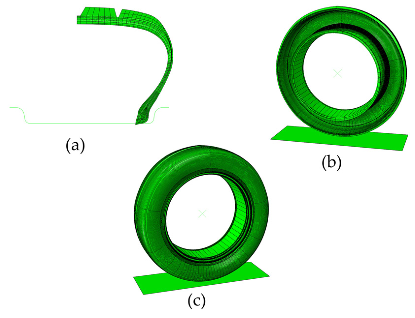
The tire is a complex structure composed of various materials, such as nylon, rubber, and steel wire. In order to reduce the complexity of finite element modeling, this paper simplifies the tire model on the basis of fully considering the purpose of the proposed research. As shown in Figure 1, carcass rubber, inner liner, bead, canopy ply, tread, carcass ply, apex, etc., is included. As shown in Figure 2, the tire modeling can be divided into three parts: (a) the establishment of the semi-2D cross-section model; (b) the semi-2D cross-section model is rotated into a semi-3D tire model; (c) the semi-3D tire model is transformed into a full 3D tire finite model though symmetrical operation. The above three steps are related by restarting analysis, and the information, such as stress and strain, is transmitted through the result transmission function, which can effectively reduce the modeling and simulation time.
2.2. Material Model and Sensor Positioning
The reinforcement layer of the tire model in this paper is composed of nylon and steel wire. Nylon and steel wire are linear materials, and the material properties can be set by defining the material’s density, Young’s modulus and Poisson’s ratio. However, rubber material is a complex nonlinear material with very complex mechanical properties. Therefore, it is not feasible to set the rubber material by the method of linear elastic material. In this paper, the rubber material is defined by the rubber constitutive model provided by ABAQUS. After fully considering the characteristics of the model and the actual deformation of the rubber, the neo-Hooke constitutive model was finally selected. This rubber constitutive model mainly has the following two advantages: (1) there is only one material parameter; (2) it has the characteristics of unconditional stability. As shown in Figure 3, the reinforcing layer of the tire includes carcass ply, cap ply and steel wire layer.
As shown in Figure 4, the triaxial accelerometer is mounted on the longitudinal centerline of the tire inner liner. It is worth noting that this paper does not model the accelerometer but uses a virtual accelerometer to collect acceleration information, that is, read the acceleration signals of the target node in the x, y and z axis directions in its local coordinate system.
3. Verification of the Tire Finite Element Model
3.1. Statics Experiment Verification
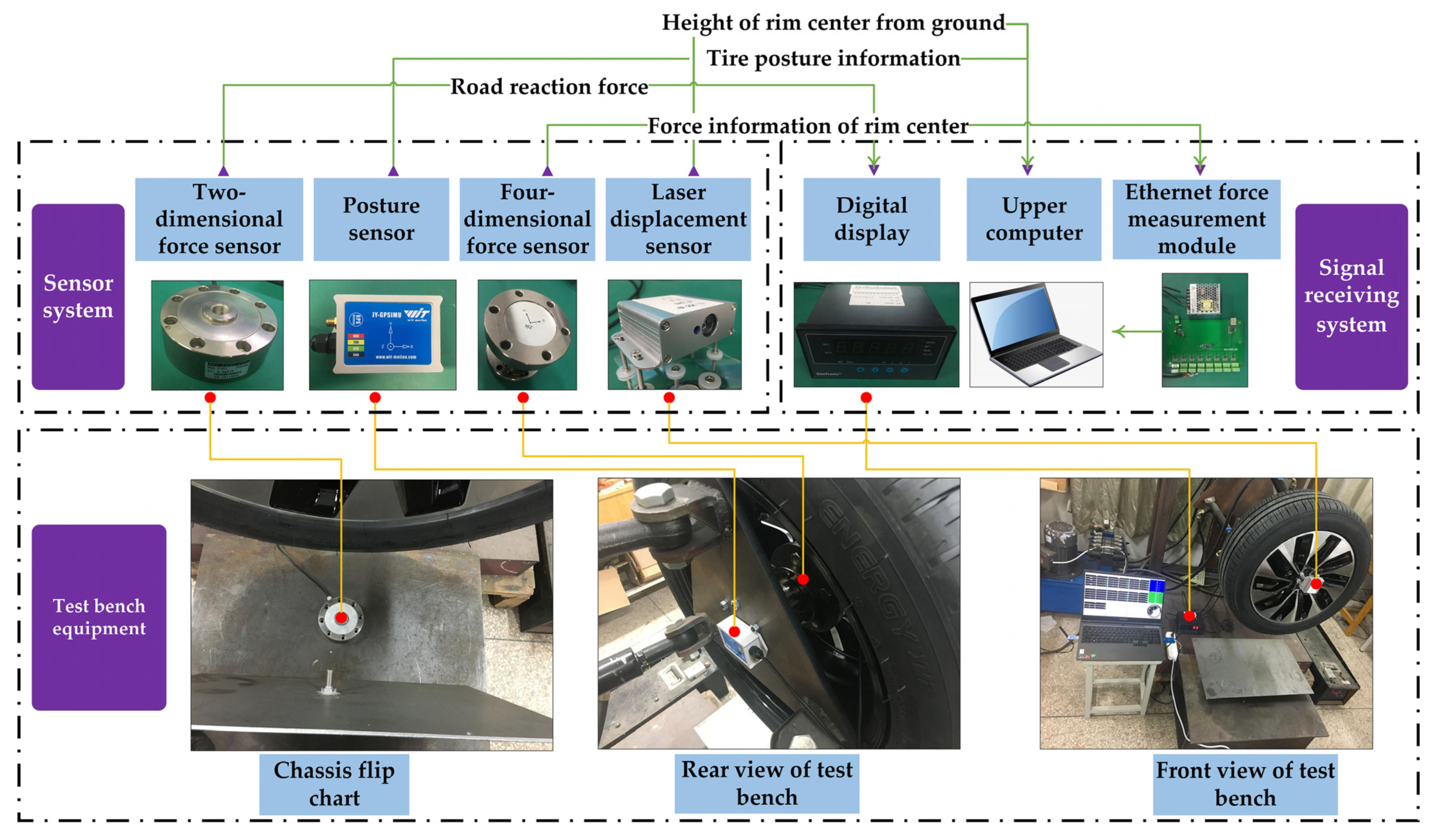
The general framework of the finite element tire model verification system built in this paper is shown in Figure 5, including test bench equipment, sensor system and signal receiving system. The test bench is composed of the main body of the bench and the test tire. The power source of the test bench is a hydraulic device. The test tire is installed on the test bench, and the camber angle of the tire and the vertical distance between the tire and the ground are adjusted through the control box. The sensor system consists of a two-dimensional force sensor, attitude sensor, four-dimensional force sensor and laser displacement sensor. The upper end face of the two-dimensional force sensor is connected to the base plate through bolts, and the lower end face is fixed on the support structure. The upper end face of the base plate is in contact with the tire surface, and the load of the tire is monitored in real time and the value is displayed through a digital display, the unit is N. The attitude sensor is installed on the tripod of the experimental bench to monitor the camber angle of the tire in real time. One end of the four-dimensional force sensor is rigidly connected to the rim, and the other end is rigidly connected to the tripod of the test bench, and the force at the center point of the rim under different vertical displacements is monitored in real time. The laser displacement sensor is installed on the center of the rim, and its laser emission point and the center of the rim are on the same horizontal line, which can realize real-time monitoring of the distance between the center of the rim and the base plate. The upper computer receives and stores the signals of the attitude sensor, the four-dimensional force sensor and the laser displacement sensor.
The radial stiffness of the tire is a very important parameter in the mechanical properties of the tire, which determines the load-bearing capacity of the tire. Therefore, the paper verifies the validity of the finite element model by comparing the radial stiffness curves of the finite element tire and the test tire. Firstly, the road surface is constrained with six degrees of freedom. Secondly, the radial loading of the rim is increased. Finally, the radial stiffness curve is obtained by extracting the radial reaction force of the four-dimensional force sensor at the center of the rim and the displacement of the center of the rim. As shown in Figure 6, the radial stiffness simulation curve of the tire is in high consistency with the test curve, which proves the validity of the tire finite element model. The specific experimental steps are as follows:
- (a)
- Set tire inflation pressure; the inflation pressure range is 0.181 MPa to 0.281 MPa.
- (b)
- Adjust camber angle to 0° through the attitude sensor and the test bench controller.
- (c)
- Control the tire to move toward the bottom plate until the tire tread lightly touches the bottom plate, at this moment the pressure exerted by the tire on the road surface is 0 N.
- (d)
- Record the distance from the center of the rim to the bottom plate at this moment.
- (e)
- Use the controller to control the tire to move down, and simultaneously record the distance between the tire and the ground and the radial reaction force of the four-dimensional force sensor at the center of the rim.
- (f)
- Draw the radial stiffness curve.
3.2. Dynamic Experiments Validation
In this paper, the accelerometer is glued to the center of the inner liner of the tire as shown in Figure 7a. The acceleration sensor is connected to the input wire of the slip ring as shown in Figure 7b through the wire running through the rim. The output end of the slip ring is connected to the signal processing and receiving equipment. The dynamic test of the finite element model designed in this paper mainly compares the acceleration signals in the tangential, lateral and longitudinal directions of the experimental and simulated tires under free rolling conditions. Both simulations and tests are executed at an inflation pressure of 0.24 MPa, a velocity of 30 km/h and a slip angle of 0°. The adhesion coefficient of the road can be regarded as 0.5, so the road friction coefficient is set to 0.5 in the simulation program.
The simulated and measured tangential graph shown in Figure 8a demonstrates that the magnitude of the tangential acceleration is almost 0 until the tire reaches the contact path. When the sensor enters and leaves the contact patch, the magnitude of the tangential acceleration increases in the opposite direction. The laws of simulation and experimental graphs are similar.
Simulated and experimental graphs as shown in Figure 8b, when the sensor enters and leaves the contact patch, the magnitude of the lateral acceleration signal increases in the same direction. It is worth noting that the maximum value of lateral acceleration is smaller than that of the radial acceleration and tangential acceleration under the same working conditions. The law of simulation curve is consistent with the experimental curve.
As shown in the simulated and experimental graphs in Figure 8c, when the sensor reaches and leaves the contact path, the rate of change of the acceleration value of the sensor is maximum. The law of the simulation curve is consistent with the experimental curve.
4. Simulation Results and Discussion
4.1. The Influence of Different Inflation Pressures on the Contact Patch
In this section, the tire load is 3000 N, the speed is 30 km/h and the tread wear is 0 mm, and the range of inflation pressure is [0.181 MPa, 0.241 MPa]. It is worth noting that the paper mainly studies the length of the longitudinal contact path of the tire, which is read by the Path function in the ABAQUS software. The red line path shown in the 0.181 MPa contact pressure (cpress) cloud diagram, as shown in Figure 9, is the path of the path node. The following also mainly studies the variation law of the contact pressure on this path. The maximum cpress is mainly distributed in the contact area center of the tire. When the inflation pressure is 0.181 MPa, the maximum cpress is 0.3156 MPa, and when the inflation pressure is 0.241 MPa, the maximum contact pressure is 0.398 MPa, as shown in Figure 9. When the inflation pressure is 0.181 MPa, the ground contact shape of the tire is similar to a rectangle, the length of the rectangle in the longitudinal and transverse directions decreases with the increase of inflation pressure, the shape of the contact area is approximately oval when the inflation pressure is 0.241 MPa as shown in Figure 9 and Figure 10. The reason is that the increase of the inflation pressure leads to the increase of the overall stiffness of the tire. It can be seen from Figure 9 and Figure 11 that the change of inflation pressure does not cause the change of cpress distribution; however, the cpress value in the central area of the contact patch increases with the increase of inflation pressure. This is due to the tire load remaining unchanged, while the ground area continues to decrease, resulting in cpress increasing. It can be seen from Figure 12 that the peak value of radial displacement decreases with the increase of inflation pressure, due to the stiffness of the tire increase with the inflation pressure. It is worth noting that the radial displacement curve is obtained by double integrating the radial acceleration curve.
4.2. The Influence of Different Loads on the Contact Patch
In this section, the inflation pressure is 0.241 MPa, the speed is 30 km/h, the tread wear is 0 mm, and the range of the load is 500 N to 3500 N. As shown in Figure 13, when the load is 500 N, the tire-ground contact area is elliptical, both the long and short axes of the ellipse increase with the load increases. When the load is 2000 N, the shape of ground area is approximately rectangular. When load is 500 N, the maximum of cpress is 0.3557 MPa, and when the load is 2000 N, the maximum is 0.4007 MPa. It can be seen from Figure 13 and Figure 14 that with the increase of the tire, the tire–ground contact area and the longitudinal length of the contact patch have a larger increase. In addition, it can be seen from Figure 14 that there is a significant linear relationship between the tire load and the longitudinal length of the ground area. It can be seen from Figure 13 and Figure 15 that with the increase of the load, the extreme value of the ground stress in the grounding area is still symmetrically distributed on both sides of the middle longitudinal groove but only increases in the longitudinal length. It is worth noting that when the load increases to 1500 N, the cpress value in the central area of the ground trace shows a decreasing trend. This is due to the stress on the tire shoulder gradually increases with the increase of the load, resulting in a “warping” phenomenon of the tread in the tire contact area, which eventually leads to a decrease in cpress. As shown in Figure 16, the maximum value of the radial displacement increases with the increase of the load.
4.3. The Effect of Different Speeds on the Contact Patch
In this section, the inflation pressure is 0.241 MPa, the load is 3000 N, tread wear is 0 mm and the range of the speed is [20 km/h, 50 km/h]. As shown in Figure 17, under the same inflation pressure and load, the free rolling speed increases from 20 km/h to 50 km/h, the maximum cpress of the tire contact area increase form 0.3986 MPa to 0.39 MPa and the cpress at the center of the ground is greater than the cpress on both sides. The longitudinal axis of the tire contact patch becomes slightly longer as the speed increases. It can be seen from Figure 17 and Figure 18 that the vehicle speed has little effect on the tire contact area and the length of the longitudinal contact patch. The values of which increased slightly with the increase of the vehicle speed, the main reason being that the increase of the vehicle speed would lead to the increase of the centrifugal force of the tire, which led to the increase of the deformation amount of the tire–ground contact surface. It can be seen from Figure 17 and Figure 19 that the change of vehicle speed does not cause the change of cpress distribution, but the cpress in the central part of the contact area decreases slightly with the increase of vehicle speed. The main reason for this is that the tire load is constant and the contact surface area increases slightly with the increase of vehicle speed, resulting in a small decrease in cpress. As shown in Figure 20, the speed of the tire has little effect on the radial displacement.
4.4. The Effects of Different Wear Amounts on the Contact Patch
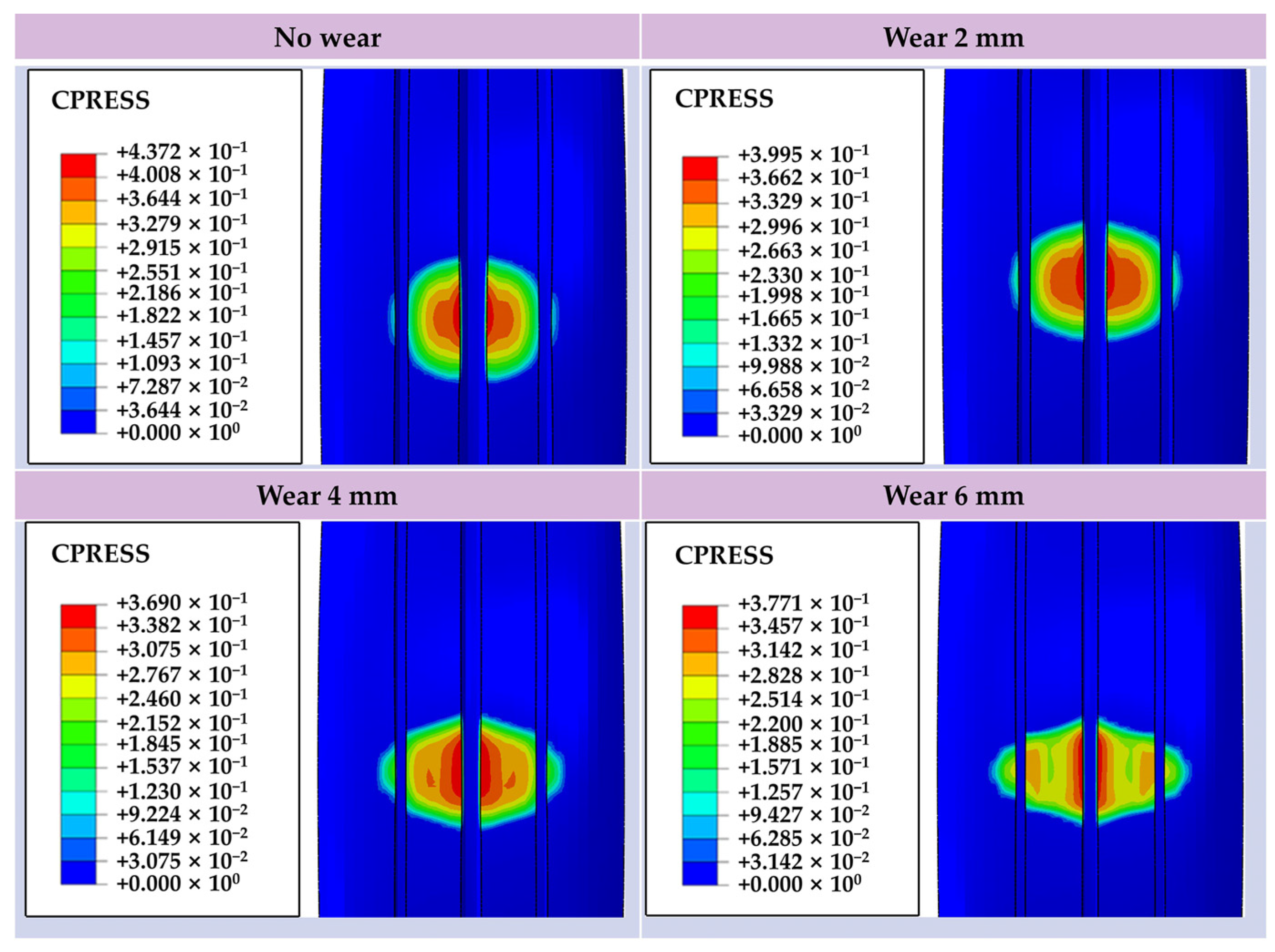
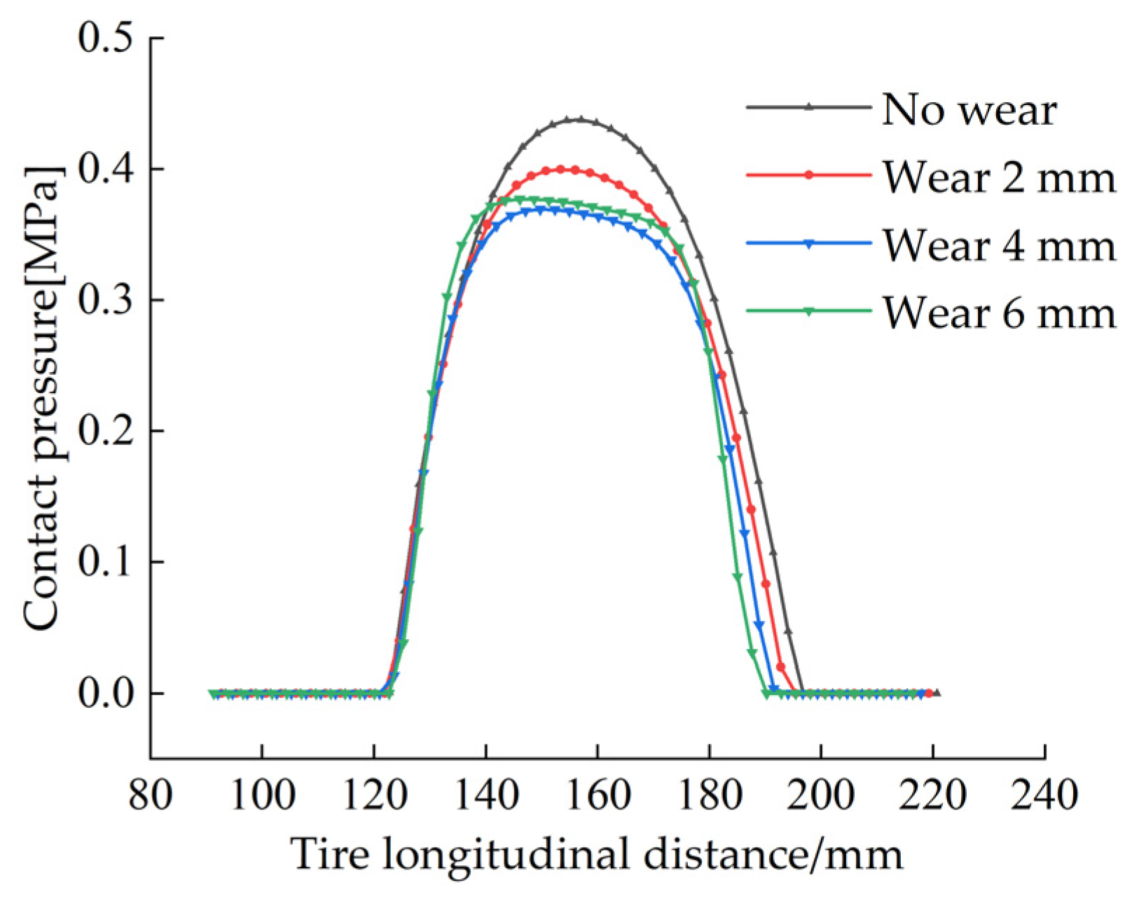
In this section, the inflation pressure is 0.241 MPa, the load is 3000 N and speed is 30 km/h. The thickness of the tire tread is total 8 mm and the paper only takes into account the change in the geometry without considering the change in the mechanical properties. Assuming that tire is uniformly worn, the range of the amount of tread wear is [0, 6 mm]. When the wear amount is 0 mm, the shape of the tire is similar to an ellipse, and the long axis of the ellipse slightly increases with the increase of wear amount and the short axis decreases slightly, as shown in Figure 21. It can be seen from Figure 21 and Figure 22 that with the increase of the tire wear amount, the ground contact area of the tire generally tends to increase. The length of the tire longitudinal contact patch decreases as the amount of tire wear increases. This is due to the tire radius decrease as the amount of tire tread wear increases, while the contact angle does not change, resulting in a decrease in the length of the longitudinal contact patch. It can be seen from Figure 20 and Figure 23 that cpress does not change regularly with the change of the wear. It may be caused by changes in the curvature of the tire as it wears. It can be seen from Figure 24 that the change of the tread wear amount has little effect on the radial displacement signal.
5. Vertical Force Prediction
5.1. Determination of Input Characteristic Parameters
From the analysis in Section 3, it can be clearly seen that the length of the longitudinal contact patch is not only affected by the inflation pressure, speed and load but also changes with the change of the amount of tread wear; however, the tire vertical force prediction algorithm in the existing literature does not consider the influence of tread wear. In addition, it can also be seen from the above analysis that the radial displacement signal at the virtual acceleration sensor is only affected by the load and inflation pressure. If the vertical force prediction algorithm is built with the radial displacement signal as the reference signal, the consideration of the influence of vehicle speed and tread wear on the prediction accuracy can be omitted, so as to simplify the input characteristic parameters and reduce the computational complexity. In order to reflect the superiority of the proposed algorithm, three estimation models, as shown in Table 2, are established in this paper. The inflation pressure and speed can be obtained directly through the vehicle sensors, the length of the longitudinal contact patch can be estimated indirectly through the acceleration signal collected by the virtual acceleration sensor, and the method for estimating the amount of tread wear has been introduced in detail in the literature [20]. The method for estimating the length of the tire longitudinal contact patch is described below.
5.2. Estimation of the Length of the Longitudinal Contact Patch Length
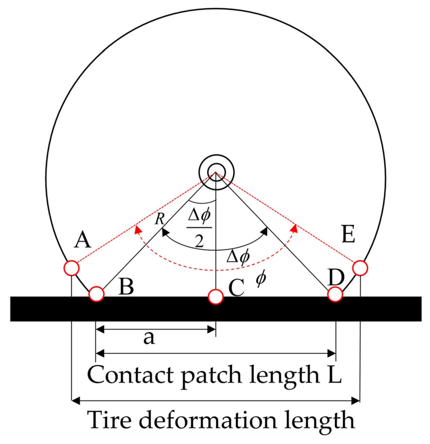
Figure 25 is the deformation diagram of the tire under the action of vertical force, is the tire contact angle, and its calculation formula can be expressed as:
In the formula, is the time required for the virtual acceleration sensor to roll through a circle, is the time required for the virtual acceleration sensor to pass through the touchdown area. At this time, the longitudinal length of the tire contact patch can be expressed as:
In the formula, is the free radius of the tire.
At this time, the problem of solving the longitudinal contact patch length of the tire is transformed into the problem of solving and . Points “B” and “D” of the ground contact pressure in Figure 26 have the same meaning as the Points “B” and “D” in Figure 25, that is, the tire longitudinal contact patch length. At the same time, it can be seen from the Figure 26 that the time interval between the first peak value and the second peak value of the radial acceleration signal is the closest to the time interval between points “B” and “D”, so the radial acceleration is selected as the reference signal for calculating . As shown in Figure 27, the time interval between the minimum values of the two radial acceleration periodic signals is selected as the total time for the tire to roll one circle. So far, the combination of formula (2) can realize the real-time calculation of the longitudinal length of the contact patch during the tire rolling process. Figure 28 shows the results of estimating the longitudinal length of the tire contact patch under different inflation pressures, loads, speeds and tread wear. The results show that the average absolute error of the longitudinal contact patch length estimation is 0.64 mm, indicating that the estimation method has high estimation accuracy and robustness is good.
5.3. Vertical Force Calculation Algorithm Based on GA-BP Neural Network Algorithm
Because the tire has a dual nonlinear structure of material nonlinearity and contact nonlinearity, it is difficult to establish an expression of the relationship between the eigen-value and the predicted value through a general mathematical formula. The neural net-work, especially the BP neural network, has a strong ability to deal with nonlinear problems. Therefore, the BP neural network is selected to establish the vertical force prediction algorithm.
- (1)
- BP neural network
The BP (back propagation) neural network is a multi-layer feedforward neural network trained according to the error back propagation algorithm, which includes input layer, hidden layer and output layer [21]. The BP neural network uses the gradient descent method for correction to achieve the accurate fitting of the data, so the BP neural network is a tutor-type learning algorithm [22]. The operation process of BP neural network is divided into two stages:
- (a)
- The forward propagation of the data flow, from the input layer through the hidden layer, finally reaches the output layer;
- (b)
- The back-propagation of the error, from the output layer to the hidden layer and finally to the input layer, constantly adjusts the weights and thresholds of each layer, when the error of the network output is reduced to the accuracy set according to a certain rule or reaches the set number of learning times stop.
The BP neural network is a commonly used back-propagation neural network model, and its structural model and the number of neurons need to be determined according to the actual situation. The predicted parameter in this paper is the vertical force, so the number of output nodes is 1. As mentioned above, the tire is a typical nonlinear system, and a three-layer BP neural network has the ability to approximate any nonlinear function [23] in theory. So, the number of hidden layers of all prediction models based on BP neural network is set to 1. The range of hidden layer nodes can be obtained by empirical formula (3).
where is the number of input nodes, is the number of output nodes, and is constant from 1 to 10. The value range of model 1~3 is [3, 12], [3, 13] and [2, 11], respectively. Finally, the number of nodes in the hidden layer of each model is determined by the traversal algorithm with the mean square error (MSE) as the selection criterion. The smaller the MSE value, the better the BP neural network fits. Figure 29 shows the relationship between the MSE value and the number of hidden layer points. It can be seen from the figure that when the number of hidden layer nodes in Prediction Models 1 to 3 is 5, 4 and 9, respectively, the corresponding MSE values are the smallest. The neural network model of the completed tire vertical force estimation is shown in Figure 30. In this paper, the sigmoid tangent function is selected as the activation function of the hidden layer, the input layer selects the function and the training function is . The neural network formula is as follows:
where is the excitation unit of the hidden layer; is the number of neurons in the hidden layer; is the transfer function of the hidden layer, its mathematical expression is ; is the weight of the neuron from the output layer to the hidden layer; is the input parameters; is the neuron threshold of the hidden layer; is the output unit, namely the vertical force; input layer activation function is , its mathematical expression is ; is the weight of the neuron from the hidden layer to the output layer. It is worth noting that when , is the threshold of the output neuron.
The value of the weight matrix between neurons is finally determined by the learning and training of the network, and it is distributed in the interval (−1, 1). The random number generation method is adopted to assign the initial value to the weight matrix. The target error of the neural network is set to 4 × 10⁻⁵. In order to avoid the outcome where the result cannot be obtained due to the long-term calculation failure during the training process, the upper limit of the number of model iterations is set to 10,000 times. At the same time, in order to prevent overfitting by affecting the accuracy of the predicted data, the maximum number of verifications of the neural network is set to 6. The training result is easily affected by the learning rate of the neural network. If the learning rate is too large or too small, it will cause the neural network to “oscillate” or reduce the convergence speed, its value is usually between 0.01 and 0.2. So, the learning rate is set to 0.1 in this paper. Finally, the parameters of the BP neural network model are shown in Table 3.
- (2)
- Genetic Algorithm (GA)
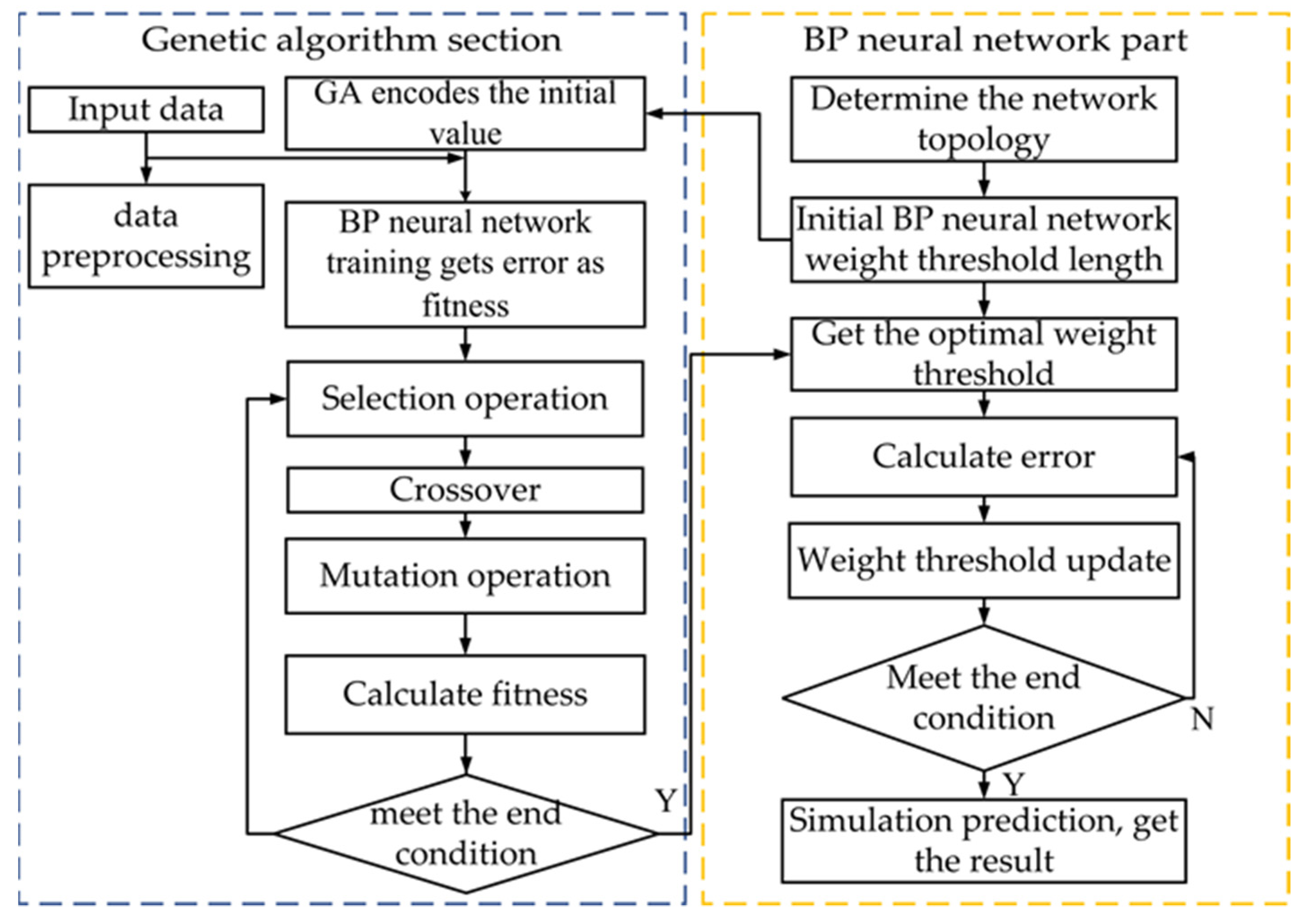
The genetic algorithm was proposed by John Holland in the United States in the 1970s. The genetic algorithm is modeled on the theory of biological evolution, which has the biological characteristics of the survival of the fittest and the survival of the fittest in the natural environment [24]. It simulates the phenomenon of biological selection, mating and mutation, can adaptively learn the optimal solution, has good global search ability and robustness and is suitable for complex nonlinear solving problems [25]. The initial weights and thresholds of the traditional BP neural network are assigned by the random assignment method, so the network falls into a local minimum during the training process and a local optimal solution will appear, so that the global optimal cannot be achieved. Therefore, this paper uses the Genetic Algorithm to optimize the BP neural network and uses the powerful global optimal search ability of the genetic algorithm to make up for the defect that the BP neural network is easy to fall into local minima. The basic algorithm flow of GA-BP neural network is shown in Figure 31.
The BP neural network method of genetic algorithm optimization is mainly composed of three parts: the establishment of BP neural network, the optimization of genetic algorithm and the prediction of BP neural network. The steps for GA to optimize BP are as follows:
- (1)
- Calculation of fitness function
The weights and thresholds of the population are obtained through the BP neural network, the expected output is denoted as , and the predicted output is denoted as , then the individual fitness is:
In the formula, is the number of output nodes; is the expected value of the node; is the predicted output of the node; is the selection coefficient.
- (2)
- Select operation
Based on the characteristics of the research object, the operation method selected in this paper is the roulette method and its formula is as follows:
In the formula, is the fitness of the individual ; is the fitness function of the individual ; is the selection coefficient; is the total number of individuals in the population.
- (3)
- Crossover operation
The encoding method used by the GA algorithm in the calculation process is real number encoding, so this paper adopts the real number crossover method, and its formula is as follows:
In the formula, is the maximum fitness in the current population; is the fitness value of the individual to be crossed; is the average fitness value of the current population; the fitness value of the individual to be mutated is recorded as . Of these, , . The final parameters of the genetic algorithm used in this paper are shown in Table 4.
5.4. Analysis of the Estimation of Tire Vertical Force Results
In this paper, the total number of data samples is 200 groups, and the proportions of the training set, validation set and test set are 70%, 20% and 10%. The mean absolute error () and the mean absolute percentage error () are used to evaluate the vertical force prediction methods of the three models. The formulas are as follows:
In the formula, is data sample; the predicted value of the network model is recorded as ; the actual value of the test data is recorded as ; the total number of samples is .
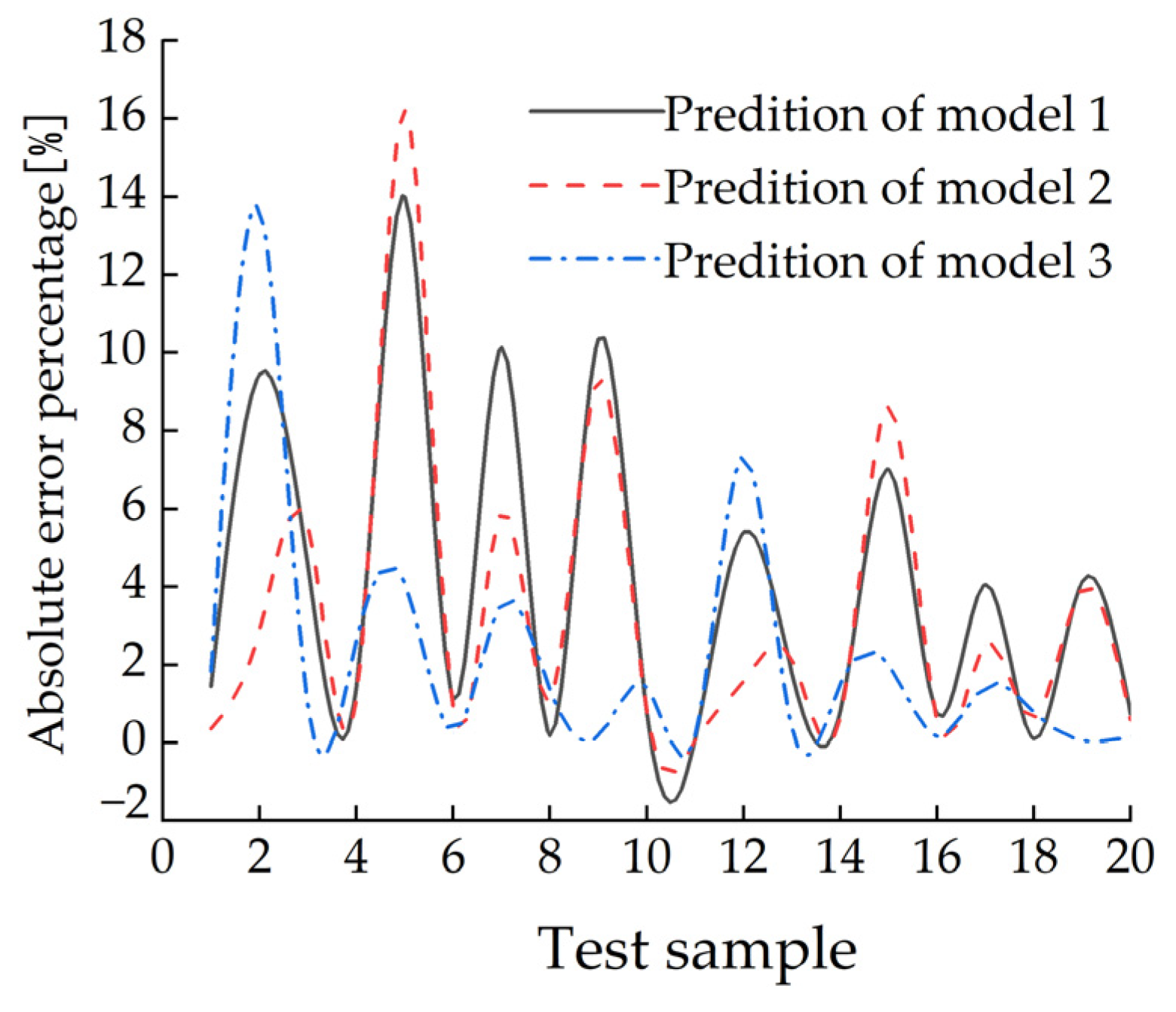
It can be seen from Figure 32 and Figure 33 and Table 5 that the prediction effect of Prediction Model 1 is the worst, due to it ignores the effect of wear on the contact path length. Prediction Model 2 takes into account the effect of wear on the length of the contact patch on the basis of Prediction Model 1, so the accuracy of Prediction Model 2 is higher than that of Prediction Model 1. Prediction Model 3 replaces the tread wear and contact path length of the input parameters with the peak value of radial displacement that is not affected by wear, which makes the structure of the prediction model simpler, improves the prediction accuracy and reduces the calculation time.
In summary, the prediction accuracy of Prediction Model 3 is the highest and the calculation time of Prediction Model 3 for the test set is also the shortest, indicating that its computational complexity is the lowest, and it is more suitable for practical engineering applications.
Next, the paper studies the formulation process of the tire vertical estimation Model 3. It can be seen from Figure 28 that the tire vertical force prediction algorithm built in this paper is a three-layer network structure, so the general formula of the tire vertical force prediction model in this section can be written as:
where and represent the thresholds from the input layer to the hidden layer and the hidden layer to the output layer, respectively; and represent the weights from the input layer to the hidden layer and from the hidden layer to the output layer; represents the transfer function; represents the input parameter. If the effects of normalization and denormalization are considered, the general formula of the tire longitudinal force prediction model in this section can be further written as:
where represents inflation pressure, represents the peak of the radial displace-ment.
6. Conclusions
- (1)
- The effects of different inflation pressure, speed, load and wear amount on the length of the longitudinal contact patch and the radial displacement at the virtual acceleration sensor are analyzed. The simulation results show that the length of the longitudinal contact patch decreases with the increase of inflation pressure and wear amount and increases with the increase of speed and load. The peak value of the radial displacement wave decreases with the increase of tire pressure and increases with the increase of load, but it is independent of the amount of tread wear and speed.
- (2)
- It was found that the radial acceleration signal of the virtual triaxial acceleration sensor has the highest correlation with the longitudinal length of the tire contact patch. The calculation method of the longitudinal contact patch length built with this signal has high prediction accuracy and good robustness. The mean absolute error is 0.64 mm.
- (3)
- According to the different input characteristic parameters, three vertical force prediction models based on GA-BP neural network algorithm are established. The inputs of Model 1 are inflation pressure, speed and length of longitudinal contact patch; Model 2 considers the influence of tread wear on the basis of Model 1, and its input features are inflation pressure, speed, length of longitudinal contact patch and tread wear. The input quantities of Model 3 are the peak value of radial displacement and inflation pressure. The mean absolute error, mean absolute error percentage and computation time of the three forecasting models were compared. The prediction results show that the three evaluation indicators of the Prediction Model 3 are all optimal, which are more suitable for practical engineering applications, and can further improve vehicle safety, handling stability, fuel economy and ride comfort.
Author Contributions
Conceptualization, T.G.; methodology, T.G.; software, T.G.; validation, T.G., B.L. and Z.Q.; re-sources, B.L. and G.Y.; data curation, T.G. and J.G.; writing—original draft preparation, B.L.; writing—review and editing, X.H. and G.Y.; supervision, S.B. and X.Z.; funding acquisition, B.L. and S.B. All authors have read and agreed to the published version of the manuscript.
Funding
This research was funded by the National Natural Science Foundation of China Youth Program 51705220; the National Natural Science Foundation of China, grant number 52172367; the Natural Science Foundation of the Jiangsu Higher Education of China, grant number 21KJA580001; and the Postgraduate Research & Practice Innovation Program of Jiangsu Province grant number XSJCX21_17.
Institutional Review Board Statement
Not applicable.
Informed Consent Statement
Not applicable.
Data Availability Statement
Not applicable.
Conflicts of Interest
The authors declare no conflict of interest.
References
- Wang, G.L.; Han, T.; Zhou, H.C.; Ding, J.J. Vertical Force Estimation Algorithm of Intelligent Tires Based on Physical Model. Automot. Eng. 2021, 43, 1865–1870. [Google Scholar]
- Rajendran, S.; Spurgeon, K.S.; Tsampardoukas, G.; Hampson, R. Estimation of road Frictional Force and Wheel Slip for Effective Antilock Braking System (ABS) Control. Int. J. Robust 2019, 29, 736–765. [Google Scholar] [CrossRef] [Green Version]
- Khaleghian, S.; Emami, A.; Taheri, S. A Technical Survey on Tire-Road Friction Estimation. Friction 2017, 5, 123–146. [Google Scholar] [CrossRef] [Green Version]
- Rezaeian, A.; Zarringhalam, R.; Fallah, S.R.; Melek, W.; Khajepour, A.; Chen, S.K.; Moshchuck, N.; Litkouhi, B. Novel Tire Force Estimation Strategy for Real-time Implementation on Vehicle Applications. IEEE Trans. Veh. Technol. 2014, 64, 2231–2241. [Google Scholar] [CrossRef]
- Cho, W.; Yoon, J.; Yim, S.; Koo, B.; Yi, K. Estimation of Tire Forces for Application to Vehicle Stability Control. IEEE Trans. Veh. Technol. 2009, 59, 638–649. [Google Scholar]
- Doumiati, M.; Victorino, A.; Lechner, D.; Baffet, G.; Charara, A. Observers for vehicle tyre/road forces estimation: Experimental validation. Veh. Syst. Dyn. 2010, 48, 1345–1378. [Google Scholar] [CrossRef]
- Ye, H.; Liu, G.H.; Zhang, D.; Wang, Y. Estimating Longitudinal Velocity of Four-Wheel-Independent-Driving Electric Vehicle based on RKF Tire Force Estimator. Mech. Sci. Technol. Aerosp. Eng. 2017, 36, 637–642. [Google Scholar]
- Antonov, S.; Fehn, A.; Kugi, A. Unscented Kalman Filter for Vehicle State Estimation. Veh. Syst. Dyn. 2011, 49, 1497–1520. [Google Scholar] [CrossRef]
- Zhang, X.W.; Wang, F.Y. Opportunities and Challenges for Tires Intelligent Manufacturing from Smart tires. Sci. Technol. 2018, 36, 38–47. [Google Scholar]
- Garcia-Pozuelo, D.; Olatunbosun, O.; Yunta, J.; Yang, X.G.; Diaz, V. A Novel Strain-Based Method to Estimate Tire Conditions Using Fuzzy Logic for Intelligent tires. Sensors 2017, 17, 350. [Google Scholar] [CrossRef] [Green Version]
- Huang, X.J.; Zhang, F.; Zhang, S.W.; Wu, Z.Q.; We, S.; Wang, F. Vertical Load Measurement of Automotive Intelligent Tire. Automot. Eng. 2020, 42, 1270–1276. [Google Scholar]
- Zhao, J.; Lu, Y.H.; Zhu, B.; Liu, S.L. Estimation Algorithm for Longitudinal and Vertical Forces of Smart Tire with Accelerometer Embedded. Automot. Eng. 2018, 40, 137–142. [Google Scholar]
- Xu, N.; Askari, H.; Huang, Y.J.; Zhou, J.F.; Khajepour, A. Tire Force Estimation in Intelligent Tires Using Machine Learning. IEEE Trans. Intell. Transp. 2020, 23, 3565–3574. [Google Scholar] [CrossRef]
- Garcia-Pozuelo, D.; Yunta, J.; Olatunbosun, O.; Yang, X.G.; Diaz, V. A Strain-Based Method to Estimate Slip Angle and Tire Working Conditions for Intelligent tires Using Fuzzy Logic. Sensors 2017, 17, 874. [Google Scholar] [CrossRef] [PubMed]
- Tuononen, A.J.; Matilainen, M.J. Real-time Estimation of Aquaplaning with an Optical Tyre Sensor. Proc. Inst. Mech. Eng. Part D J. Automob. Eng. 2009, 223, 1263–1272. [Google Scholar] [CrossRef]
- Yilmazoglu, O.; Brandt, M.; Sigmund, J.; Genc, E.; Hartnagel, H.L. Integrated InAs/GaSb 3D magnetic field sensors for “the intelligent Tire”. Sens. Actuators A 2001, 94, 59–63. [Google Scholar] [CrossRef]
- Erdogan, G.; Alexander, L.; Rajamani, R. Estimation of Tire-road Friction Coefficient Using a Novel Wireless Piezoelectric Tire Sensor. IEEE Sens. J. 2011, 11, 267–279. [Google Scholar] [CrossRef]
- Pohl, A.; Steindl, R.; Reindl, L. The “intelligent tire” utilizing passive SAW sensors measurement of tire friction. IEEE Trans. Instrum. Meas. 1999, 48, 1041–1046. [Google Scholar] [CrossRef]
- Xu, N.; Huang, Y.J.; Askari, H.; Tang, Z.P. Tire Slip Angle Estimation Based on the Intelligent Tire Technology. IEEE Trans. Veh. Technol. 2021, 70, 2239–2249. [Google Scholar] [CrossRef]
- Li, B.; Quan, Z.Q.; Bei, S.Y.; Zhang, L.C.; Mao, H.J. An Estimation Algorithm for Tire Wear Using Intelligent Tire Concept. Proc. Inst. Mech. Eng. Part D J. Automob. Eng. 2021, 235, 2712–2725. [Google Scholar] [CrossRef]
- Yang, Y.; Gao, J.; Gu, Z.Q.; Liu, Z.Z.; Zheng, L.D. Research on Sound Quality Prediction Model of Automobile Wind Buffeting Noise Based on GA-BP. Chin. J. Mech. Eng. 2021, 57, 241–249. [Google Scholar]
- Singh, K.B.; Taheri, S. Accelerometer based Method for Tire Load and Slip angle Estimation. Vibration 2019, 2, 174–186. [Google Scholar] [CrossRef] [Green Version]
- Zhou, M.; Lü, Z.G.; Di, R.H.; Li, Y. BP Neural Network Modeling Based on Small Sample Data. Sci. Technol. Eng. 2022, 22, 2754–2760. [Google Scholar]
- Zheng, D.; Qian, Z.D.; Liu, Y.; Liu, C.B. Prediction and Sensitivity Analysis of Long-Term Skid Resistance of Epoxy Asphalt Mixture Based on GA-BP Neural Network. Constr. Build. Mater. 2018, 158, 614–623. [Google Scholar] [CrossRef]
- Che, Y.; Xiao, W.X.; Chen, L.J.; Huang, Z.C. GA-BP Neural Network Based Tire Noise Prediction. Adv. Mater. Res. 2012, 443–444, 65–70. [Google Scholar] [CrossRef]
Figure 1.
Schematic diagram of tire model structure.

Figure 2.
205/55/R16 finite element model: (a) semi-2D tire section finite element model; (b) semi-3D tire finite element model; (c) full 3D tire finite element model.
Figure 2.
205/55/R16 finite element model: (a) semi-2D tire section finite element model; (b) semi-3D tire finite element model; (c) full 3D tire finite element model.

Figure 3.
Reinforcing layer structure of tires.

Figure 4.
Schematic diagram of the position of the three-axis accelerometer.

Figure 5.
General frame diagram of the finite element tire model verification system.

Figure 6.
Radial stiffness curve.

Figure 7.
Installation diagram of the sensor, (a) sensor location (b) experimental tire equipment.

Figure 8.
Comparison of experimental and simulation results.

Figure 9.
Contour map of tire contact pressure under different inflation pressures.

Figure 10.
Curves of tire contact area and longitudinal contact length under different inflation pressures.
Figure 10.
Curves of tire contact area and longitudinal contact length under different inflation pressures.

Figure 11.
Contact pressure distribution of tire longitudinal contact patch under different inflation pressures.
Figure 11.
Contact pressure distribution of tire longitudinal contact patch under different inflation pressures.

Figure 12.
Variation curve of radial displacement under different inflation pressures.

Figure 13.
Contour map of tire contact pressure under different loads.

Figure 14.
Curves of tire contact area and longitudinal contact length under different loads.

Figure 15.
Contact pressure distribution of tire longitudinal contact patch under different loads.

Figure 16.
Variation curve of radial displacement under different loads.

Figure 17.
Contour map of tire contact pressure at different speeds.

Figure 18.
Curves of tire contact area and longitudinal contact length at different speeds.

Figure 19.
Contact pressure distribution of tire longitudinal contact patch at different speeds.

Figure 20.
Radial displacement curves at different speeds.

Figure 21.
Contact pressure distribution of tire longitudinal contact patch under different wear amounts.
Figure 21.
Contact pressure distribution of tire longitudinal contact patch under different wear amounts.

Figure 22.
Curves of tire contact area and longitudinal contact length under different wear amounts.
Figure 22.
Curves of tire contact area and longitudinal contact length under different wear amounts.

Figure 23.
Contact pressure distribution of tire longitudinal contact patch under different wear.

Figure 24.
Radial displacement curves under different wear amounts.

Figure 25.
Deformation diagram of tire contact patch.

Figure 26.
Comparison of acceleration signal and tire contact pressure in a single cycle.

Figure 27.
Lateral acceleration signal diagram of multiple periods.

Figure 28.
Verification results of the longitudinal estimation of the tire contact patch length.

Figure 29.
The relationship between the MSE value and the number of hidden nodes.

Figure 30.
Neural network model diagram of tire vertical force estimation.

Figure 31.
Flowchart of the basic algorithm of GA-BP neural network.

Figure 32.
The vertical force prediction results of the three models.

Figure 33.
Prediction absolute error percentage of three models.


Table 1.
Experimental and simulation results of tire radial stiffness.
| Inflation Pressure (MPa) | Simulation Value (N) | Test Value (N) | Absolute Error Percentage (%) |
|---|---|---|---|
| 0.18 | 1006 | 993.3 | 1.27 |
| 0.20 | 1087 | 1091.7 | 0.43 |
| 0.22 | 1186 | 1182.3 | 0.31 |
| 0.24 | 1246 | 1224.8 | 1.73 |
| 0.26 | 1324 | 1280.5 | 3.4 |
| 0.28 | 1402 | 1353.3 | 3.6 |
Table 2.
Input characteristic parameters of each vertical force prediction model.
| Predictive Model | Input | Output |
|---|---|---|
| Predictive model 1 | Inflation pressure, speed, longitudinal contact patch length | Vertical force |
| Predictive mode 2 | Inflation pressure, speed, longitudinal contact patch length, wear amount | |
| Predictive mode 3 | Inflation pressure, radial displacement peak value |
Table 3.
BP neural network model parameters.
| Method | Parameter | The Number of Neurons in the Hidden Layer | Hidden Layer Activation Function | Output Layer Activation Function | Target Error | Iteration Upper Limit | Learning Rate |
|---|---|---|---|---|---|---|---|
| Model 1 | Value | 5 | 4 × 10⁻⁵ | 10,000 | 0.1 | ||
| Model 2 | 4 | ||||||
| Model 3 | 9 |
Table 4.
GA-BP neural network model parameters.
| Parameter Name | Parameter Value |
|---|---|
| Number of iterations | 200 |
| Population size | 60 |
| Crossover probability | 0.5 |
| Mutation probability | 0.05 |
Table 5.
Summary of the prediction results of the three prediction models on the test set.
| Predictive Model | Input | MAE(N) | MPAE (%) | Calculation Time |
|---|---|---|---|---|
| Model 1 | Inflation pressure, speed, longitudinal contact patch length | 75.73 | 3.9% | 0.031 |
| Model 2 | Inflation pressure, speed, longitudinal contact patch length, wear amount | 64.60 | 3.3% | 0.033 |
| Model 3 | Inflation pressure, radial displacement peak value | 47.55 | 2.2% | 0.021 |
Publisher’s Note: MDPI stays neutral with regard to jurisdictional claims in published maps and institutional affiliations. |
© 2022 by the authors. Licensee MDPI, Basel, Switzerland. This article is an open access article distributed under the terms and conditions of the Creative Commons Attribution (CC BY) license (https://creativecommons.org/licenses/by/4.0/).
Share and Cite
MDPI and ACS Style
Gu, T.; Li, B.; Quan, Z.; Bei, S.; Yin, G.; Guo, J.; Zhou, X.; Han, X. The Vertical Force Estimation Algorithm Based on Smart Tire Technology. World Electr. Veh. J. 2022, 13, 104. https://doi.org/10.3390/wevj13060104
AMA Style
Gu T, Li B, Quan Z, Bei S, Yin G, Guo J, Zhou X, Han X. The Vertical Force Estimation Algorithm Based on Smart Tire Technology. World Electric Vehicle Journal. 2022; 13(6):104. https://doi.org/10.3390/wevj13060104
Chicago/Turabian StyleGu, Tianli, Bo Li, Zhenqiang Quan, Shaoyi Bei, Guodong Yin, Jinfei Guo, Xinye Zhou, and Xiao Han. 2022. "The Vertical Force Estimation Algorithm Based on Smart Tire Technology" World Electric Vehicle Journal 13, no. 6: 104. https://doi.org/10.3390/wevj13060104