Article

Spatio-Temporal Dynamics of crAssphage and Bacterial Communities in an Algerian Watershed Impacted by Fecal Pollution

by
Dalal Boulainine
1,2,
Aziz Benhamrouche
3,†,
Elisenda Ballesté
2,4,
Samia Mezaache-Aichour
1 and
Cristina García-Aljaro
2,4,*
1
Laboratory of Applied Microbiology, Faculty of Natural and Life Sciences, University Ferhat Abbas, Sétif 1, Sétif 19137, Algeria
2
Departament de Genètica, Microbiologia i Estadística, Secció Microbiologia, Virologia I Biotecnologia, Facultat de Biologia, Universitat de Barcelona (UB), Av. Diagonal 643, 08028 Barcelona, Spain
3
Department of Earth Sciences, University Ferhat Abbas, Sétif 1, Sétif 19137, Algeria
4
Institut de Recerca de l’Aigua (IDRA), Universitat de Barcelona (UB), C. Montalegre, 6, 08001 Barcelona, Spain
*
Author to whom correspondence should be addressed.
Current Address: Department of Territory Planning, University Constantine 1, Frères Mentouri, Campus Zouaghi Slimane, Route de Ain el Bey, Constantine 25000, Algeria.
Water 2024, 16(8), 1123; https://doi.org/10.3390/w16081123
Submission received: 12 March 2024 / Revised: 8 April 2024 / Accepted: 9 April 2024 / Published: 15 April 2024
(This article belongs to the Section Water Quality and Contamination)

Abstract

:
This study investigates the influence of urban pollution and climate dynamics on water quality and the bacterial communities in an Argelian watershed. Twenty-one sampling campaigns were conducted over two years at six sites along the Oued Boussellam, a river impacted by the effluent of a sewage treatment plant, from a low-polluted site to a water reservoir within a 50 km distance. Fecal indicators and the human fecal marker crAssphage were monitored. Illumina 16S rRNA amplicon sequencing was used to assess water microbial populations’ changes. Urban sewage discharge had an impact on the river quality and microbial ecosystem, which was attenuated along the river course. Significant reductions (>4 log10 for E. coli and somatic coliphages, >3 log10 for crAssphage) occurred, particularly during high-temperature periods. crAssphage correlated strongly with somatic coliphages downstream the river. Seasonal differences were observed in the diversity of the bacterial communities, with higher values during the high-temperature period. The genus-level community structure was similar at highly polluted river sites, also displaying seasonal differences. Despite high pollution levels, natural processes reduced fecal indicators to acceptable levels in the reservoir as well as shaped the bacterial communities along the river, highlighting the importance of understanding indicator persistence and microbial community resilience for effective water quality management within the context of the global warming scenario.

1. Introduction

Global warming is expected to significantly impact water quality, particularly in the Mediterranean region, which is considered highly vulnerable, with expected changes in the precipitation pattern throughout the year leading to shifts in rainfall distribution [1,2]. These changes can have a significant impact on the quality and availability of water during specific seasonal periods.
Water scarcity is particularly severe in regions of the world characterized by low rainfall and high evaporation rates, such as Northern Africa, including Algeria. Algeria is currently facing the challenge of rising temperatures, decreasing water availability, and deteriorating water quality, all of which have adverse effects on water production [3]. Consequently, water monitoring is essential to ensuring human access to water while minimizing the health risks associated with fecal contamination. Moreover, improvements in water management strategies are crucial for prioritizing sustainable water management practices.
Water management varies from one country to another, depending on the water resources available and regulations. The design of the sewerage system greatly affects the composition of wastewater. In many countries, especially in older urban areas, combined sewer systems are still in use. In combined sewer systems, both domestic sewage and stormwater runoff are collected in the same pipes, and during heavy rainfall events, the volume of wastewater can exceed the capacity of the treatment plants. As a result, in such cases, a portion of the combined wastewater may be discharged directly into local water bodies without undergoing treatment. This can lead to environmental pollution and poses risks to public health if not managed properly. Furthermore, the improper disposal of wastewater can often lead to irreversible losses in ecosystem productivity, such as soil salinization, and the pollution of groundwater resources [4].
Traditionally, fecal bacterial indicators (FBIs), mainly Escherichia coli or fecal coliforms and enterococci, have been used to assess the microbiological quality of water and determine the presence of fecal contamination [5,6]. Bacteriophages have been incorporated into recently developed guidelines for water quality monitoring [7,8,9]. Somatic coliphages and F-RNA phages have proved to be reliable indicators of fecal viral pollution and suitable for use in water treatment processes [10,11]. Besides FBIs, microbial source tracking (MST) markers have emerged in recent decades as important tools for water quality monitoring and management [12,13]. They allow the identification of specific sources of fecal contamination and enable the implementation of targeted management strategies to mitigate risks. They are also used to help assess potential health risks and to evaluate the effectiveness of implemented management strategies [12]. Various MST markers have been defined, including Bacteroidales-based markers like the human-associated HF183 marker and the ruminant marker Rum2Bac [14]. F-specific RNA phages have been used as indicators of the origin of fecal contamination, with GII and GIII being more frequently detected in human excreta [14,15,16,17]. These markers appear to be host specific, but they are not universal markers for application worldwide and make it necessary to test their specificity in the different locations to be implemented [18]. A recent MST marker derived from a metagenomic study identified crAssphage (crAssPH) (p-crAssphage, prototype crAssphage) as the most abundant bacteriophage in sewage that seemed to be present worldwide [19,20]. This bacteriophage is affiliated with the Intestiviridae family, species Carjivirus communis, with Bacteroides as the putative host [19,21]. Since then, other phages (crAss-like phages), similar in their genomic architecture and sharing the same ancestor with p-crAssphage, have been detected, and some of them have been isolated [22]. The potential of p-crAssphage as a human-associated MST molecular marker has been evaluated using different qPCR methods in different countries [23,24]. These assays have been successfully applied to quantify feces, wastewater, and surface water in many regions, including Europe [23,25,26], Asia [27,28], North America [29,30], South America [31], and Australia [32], among others.
In recent decades, the One Health concept has emerged as a comprehensive and integrated approach that seeks to harmonize and optimize efforts, fostering cooperation in the domains of public health, animal welfare, and environmental conservation, involving collaboration between public health authorities, veterinarians, environmental scientists, policymakers, and other stakeholders [33]. While much of the ongoing work has focused on understanding the transmission pathways of pathogens between humans and animals, in recent years, the study of water-related exposure pathways has gained interest because of its pivotal role not only in the transmission of diseases between humans and animals, but also in shaping ecosystem functions and dynamics, particularly in the context of anthropogenic pollution. Water-related exposure pathways have significant implications for human, animal, and environmental health. Understanding these pathways is essential for identifying potential sources of contamination, assessing associated risks, and implementing effective mitigation strategies. Moreover, monitoring water and wastewater systems can serve as an invaluable tool for the early detection and management of endemic diseases and potential outbreaks at the population level [34].
Different methods can be employed to study microbial populations in ecosystems to elucidate the diversity, composition, and function of microbial communities in order to understand their perturbation from an ecological point of view [35]. One common method used to study microbial diversity is 16S rRNA amplicon sequencing, which targets the hypervariable regions of the 16S rRNA gene to identify and characterize bacterial and archaeal taxa present in environmental samples. This technique allows us to identify key microbial taxa and investigate how environmental factors influence microbial composition and diversity, advancing our understanding of ecosystem processes [36].
The aim of this study was to assess the anthropogenic impact (mainly point source fecal pollution) on the microbiological water quality indicators in a watershed in Sétif (Algeria) from a One Health perspective. This region, characterized by a dry Mediterranean climate, has faced challenges in recent years, including water scarcity, rapid population growth, and an increasing number of flooding events. The sewage of this locality flows into Oued Boussellam, a stream that feeds into a dam used for drinking water production. Over a two-year period, we assessed the levels and dynamics of two FBIs (E. coli, spores of sulfite-reducing clostridia (SSRC)), a fecal viral indicator (somatic coliphages), and the human MST marker (crAssphage). Furthermore, we investigated the effect of anthropogenic pollution in the bacterial diversity and communities within the watershed to gain knowledge on the resilience of these communities in the ecosystem under different climate conditions.

2. Materials and Methods

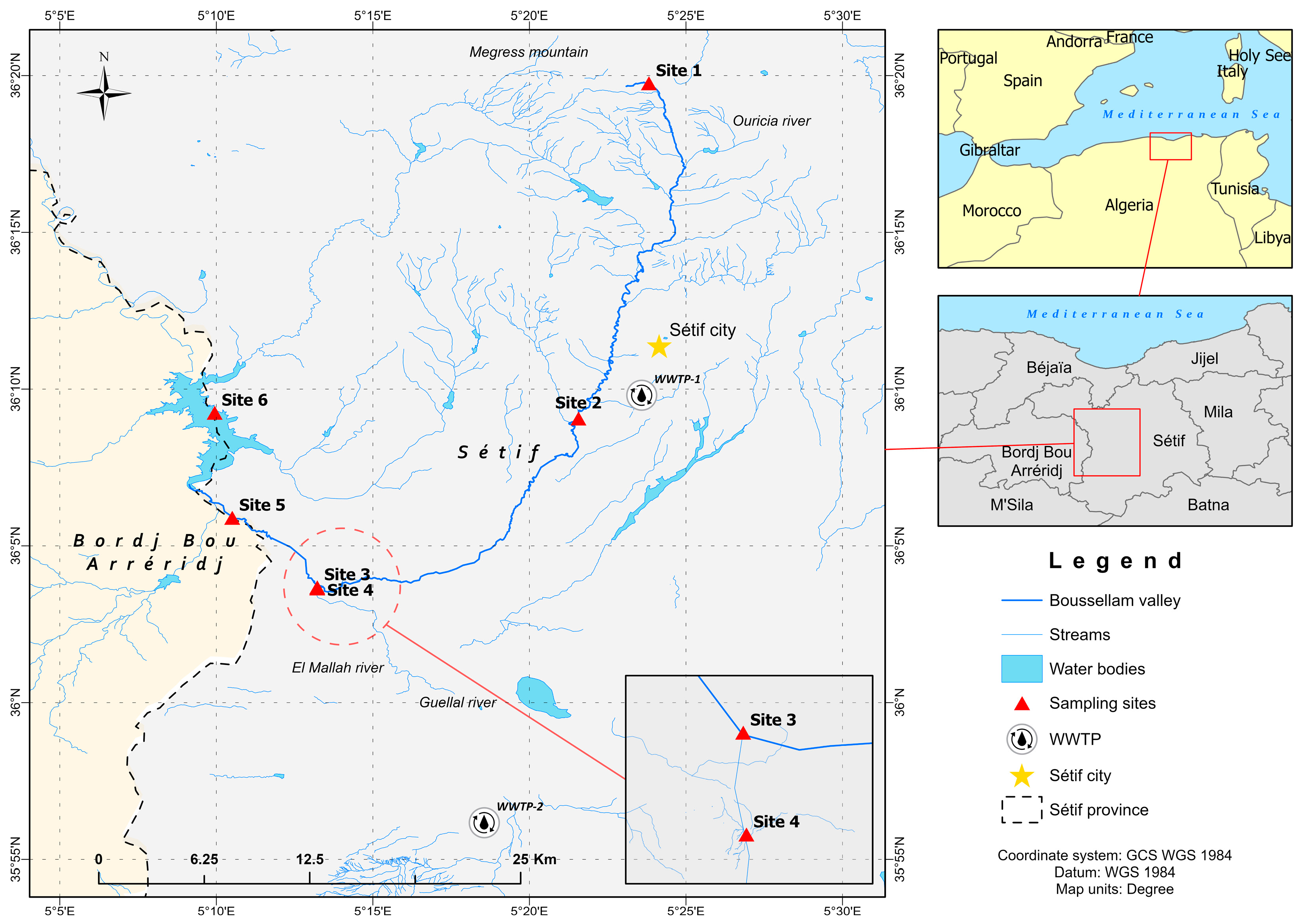
2.1. Study Area and Sample Collection

Sampling was carried out along the Oued Boussellam catchment, the main hydrographic axis of Sétif. It originates in Ras Ain Boussellam at an altitude of about 1100 m, five kilometers northwest of the town of Sétif, and flows into Oued Soummam (Figure 1). Oued Boussellam has a length of 159 km and a regulatable annual volume of nearly 38 Hm3. The catchment area is 4300 km2, and it is constituted by the confluence of the Wadi Gassar and Wadi Ouricia.
Six sampling sites along the river course were selected for the study. In the upstream–downstream direction, the first site (S1) was located upstream of Ouricia town, which has more than 25,000 inhabitants, and it is characterized by an irregular flow, drying up from late spring to early autumn, and being aligned with high temperatures. The second site (S2) was located after the town of Sétif, where sewage effluent from a wastewater treatment plant (WWTP) is discharged. The WWTP provides biological treatment using medium-load activated sludge, with aerobic stabilization. Its nominal capacity (inhabitant equivalents) is 450,000 with an average daily flow of 99,000 (m3/d) and an hourly flow rate (m3/h) of 4125, while the maximum flow capacity in dry weather is estimated at 6600 m3/h. The water treatment sector includes pre-treatment stages (rough screening, mechanical screening, sand removal/oil removal), biological treatment (two aeration basins), and secondary lamination treatment (filters). Furthermore, sludge treatment goes through stabilization, thickening, and drying stages. After these operations, the water is discharged into the Boussellam River. The third site (S3) was located downstream of Mezloug town, which has around 20,000 inhabitants. The fourth site (S4) was located at the confluence of Oued Guellal with Oued El Mallah and receives water from mostly an industrial area. The fifth site (S5) was situated 3 km before the Ain Zada reservoir, and the sixth site (S6) was at the Ain Zada Dam, a reservoir used for the production of drinking water (Figure 1). The Boussellam River and Geudjel River are the main water inflows of the Ain Zada reservoir. The catchments of these rivers are mostly covered by agricultural and residential land, which are heavily impacted by human activities.
Water samples were collected over a period of two years from November 2019 to September 2021 (n = 122). A total of 21 sampling campaigns were conducted. Samples collected at each site, as well as data on the sampling day, rainfall before the sampling day, and humidity, are summarized in Appendix A (Table A1).

2.2. Chemical Characterization of the Water

Different physical and chemical parameters describing the overall quality of surface water were recorded. These parameters included temperature, pH, electrical conductivit, measured using BIOBLOCK WTW LF 320 (Bioblock, Burladingen, Germany), turbidity measured using HACH 2100N (Hach, Dubai, United Arab Emirates), NO2 (determined using a reaction with 4-aminobenzene sulfonamide in the presence of ortho phosphoric acid to form a diazo salt that forms a pink coloring complex with the dihydrochloride amoni-4benzene sulfonamide, which is measured at 540 nm), NH4+ (determined by measuring the blue compound formed by the reaction of ammonium with salicylate and hydrochlorite ions in the presence of sodium nitropentacyanoferrate, at 650 nm), PO43− (determined by a formation in an acidic medium of a complex with ammonium molybdate and antimony and potassium double tartrate, reduction through ascorbic acid into a blue-colored complex that has two maximum absorption values, one around 700 nm and the other, more important, one at 880 nm), and total organic matter (OM), determined according to ISO 8467:1993 [37]. Water samples were collected in 1 L bottles and transported to the laboratory at 4 °C. All parameters were analyzed in the laboratory of the Algerian Water Unit (ADE) in Skikda within 24 h, using standard methods [38,39] except for temperature and pH, which were measured with a thermometer and pH meter (WTW pH 330i/SET, Weilheim, Germany) onsite. This information is shown in Appendix A (Table A2).

2.3. Enumeration of Fecal Microbial Indicators Using Culture Methods

For E. coli enumeration, different volumes of the water samples (0.001 to 100 mL) were filtered through 0.45 µm pore size cellulose ester filters (Sartorius, Goettingen, Germany). When necessary, samples were ten-fold serially diluted in phosphate-buffered saline (PBS) (pH 7.4); in this case, ten mL of the corresponding dilution were filtered. The filters were incubated upside down in Chromocult® Coliform Agar (Merck, Darmstadt, Germany). Incubation was first performed for 2 h at 37 °C to adapt potentially damaged microorganisms and then at 44 ± 0.5 °C for 20 to 22 h [40]. The results were expressed as CFU 100 mL−1.
To enumerate spores of sulfite-reducing clostridia (SSRC), volumes ranging between 0.1 mL and 7.5 mL, depending on the sample, were subjected to a thermal shock at 80 °C for 10 min. They were then anaerobically cultured through mass inoculation in Clostridium perfringens selective agar (Scharlab, Barcelona, Spain) and incubated overnight at 37 °C, as previously described [41]. The results were expressed as CFU 100 mL−1.
Somatic coliphages (SOMCPHs) were quantified by enumerating plaque-forming units (PFUs) using the host strain WG5 of E. coli in accordance with ISO 10705-2 [42] using Modified Scholten’s Agar (MSA) with the double agar layer method for the samples with high fecal pollution. Briefly, the samples were ten-fold diluted, and one mL of the corresponding decimal dilution of the sample was analyzed in duplicate with the corresponding host strain. For those samples with low fecal pollution, the single-layer agar method was used instead. For this, 100 mL of the sample was thoroughly mixed with 100 mL of double-strength semi-solid MSA and poured into 5 plates (14 cm diameter). The results were expressed as PFU 100 mL−1.

2.4. DNA Extraction

One hundred mL of each sample were concentrated using a 0.22 μm pore size cellulose ester membrane (SO-PAK, Millipore, Darmstadt, Germany), from which DNA was extracted. Membranes were placed in 0.5 mL of GITC buffer (5 M guanidine thiocyanate, 100 mM EDTA [pH 8.0], 0.5% sarkosyl) and frozen at −20 °C in lysis buffer until DNA extraction. The DNA was extracted using the QIAamp DNA Blood Mini Kit (Qiagen GmbH, Hilden, Germany) with some modifications, as previously reported [43]. Filtration and DNA extraction controls were run together with the samples. The DNA was suspended in a final volume of 100 µL of buffer AE.

2.5. Quantification of crAssphage via qPCR

Quantitative PCR amplifications were performed in 20 μL reaction mixtures using TaqMan Environmental Master Mix 2.0 (Applied Biosystems, Barcelona, Spain) in a StepOne Real-Time PCR System (Applied Biosystems). The crAssphage qPCR mixtures contained 10 μL of TaqMan Master Mix 2X, 1 μM of each primer, 250 nM of probe, and 2 μL of the DNA sample, as previously described [23]. The qPCR cycling parameters consisted of 10 min at 95 °C, followed by 40 cycles of 15 s of denaturation at 95 °C, and 60 s of annealing and extension at 60 °C. All qPCR reactions were performed in duplicate. For each qPCR run, a set of decimal dilutions of a gblock standard and a non-template control were included.

2.6. Bacterial Community Characterization

The V4 region was amplified from DNA sample extracts using the primers from the Earth Microbiome Project [515F [44] (5′-GTGYCAGCMGCCGCGGTAA-3′) and 806R [45] (5′-GGACTACNVGGGTWTCTAAT-3′)]. The PCR was performed in 25 μL of volume with a 0.2 μM primer concentration and KAPA HiFi HotStart ReadyMix (Roche Diagnostics, Barcelona, Spain). The cycling conditions were an initial denaturation of 3 min at 95 °C followed by 25 cycles of 95 °C for 30 s, 55 °C for 30 s, and 72 °C for 30 s, ending with a final elongation step of 5 min at 72 °C. After this first PCR step, water was added to a total volume of 50 μL, and reactions were purified using AgenCourt AMPure XP beads (Beckman Coulter, L’Hospitalet de Llobregat, Spain). The first PCR primers contain overhangs allowing the addition of full-length Nextera adapters with barcodes for multiplex sequencing in a second PCR step, resulting in sequencing-ready libraries with approximately 450 bp insert sizes. To do so, five μL of the first amplification was used as a template for the second PCR with Nextera XT v2 adaptor primers in a final volume of 50 μL using the same PCR mix and thermal profile as for the first PCR but only 8 cycles. After the second PCR, 25 μL of the final product was used for purification and normalization with a SequalPrep normalization kit (ThermoFisher Scientific, Barcelona, Spain), according to the manufacturer’s protocol. Libraries were eluted and pooled for sequencing. Final pool libraries were analyzed using an Agilent Bioanalyzer (Agilent Technologies, Madrid, Spain) or Fragment analyzer High Sensitivity assay (Agilent Technologies) to estimate the quantity and check the size distribution and were then quantified via qPCR using the KAPA Library Quantification Kit from KapaBiosystems (Merck, Darmstad, Germany) prior to sequencing with Illumina’s Miseq 2 × 300 bp (Illumina, San Diago, CA, USA).
Negative controls (blanks from the DNA extraction process, as well as from the DNA amplification), as well as a positive control (ZymoBIOMICS Microbial Community DNA Standard D6306, Zymo Research-Ecogen, Barcelona, Spain), were included. Sample sequencing was performed in a single run using the Illumina MiSeq platform at the Genomics Unit of Centre for Genomic Regulation Core Facilities (CRG, Barcelona, Spain).

2.7. Statistical Analyses

Colony-forming units (CFUs) and gene copy numbers were log-transformed before statistical analyses. To assess seasonal variations, samples were categorized into high- and low-temperature groups, with ‘high’ defined as minimal and maximum temperatures above 12 °C and 22 °C, respectively, corresponding mainly to the summer samples, and ‘low’ defined as below these values. Data were analyzed and visualized using the statistical software R version 4.2.2 using RStudio interface. Differences between the groups were assessed using the Mann–Whitney U test. Correlation analyses were conducted using Spearman linear correlation statistics. Spearman’s rho rank correlation coefficients ranging between 0.2 and 0.39 were classified as weak correlations; 0.4–0.59, as moderate correlations; 0.6–0.79, as strong correlations; and 0.8–1, as very strong correlations. Statistical significance was set to a p value of 0.05 for all the statistical analyses.

3. Results and Discussion

3.1. Physicochemical Parameters

The nutrient content, particularly PO43− and NH4+, were low in the less polluted water samples before the discharge of the effluent of the WWTP, with mean concentrations of 1.6 ± 1.6 mg/mL and 2.3 ± 3.6 mg/mL, respectively. However, these concentrations were increased in water samples located downstream the WWTP (S2 and S3) (4.1 ± 2.3 mg/mL, 6.9 ± 3.7 mg/mL at S2, and 4.3 ± 1.8 mg/mL, 6.7 ± 2.5 mg/mL at S3, respectively) in accordance to what has been generally reported in other rivers impacted by the effluent of WWTPs, because the effluents can still contain a high concentration of nutrients [46]. Subsequently, the concentrations decreased again, recovering to levels observed in the less impacted water samples at S5 for PO43− and S6 for NH4+, which may relate to processes such as sedimentation and/or microbial degradation. No other significant changes were observed for the other monitored parameters. The physicochemical parameters of the water samples from the different sampling sites are presented in Appendix A (Table A2).

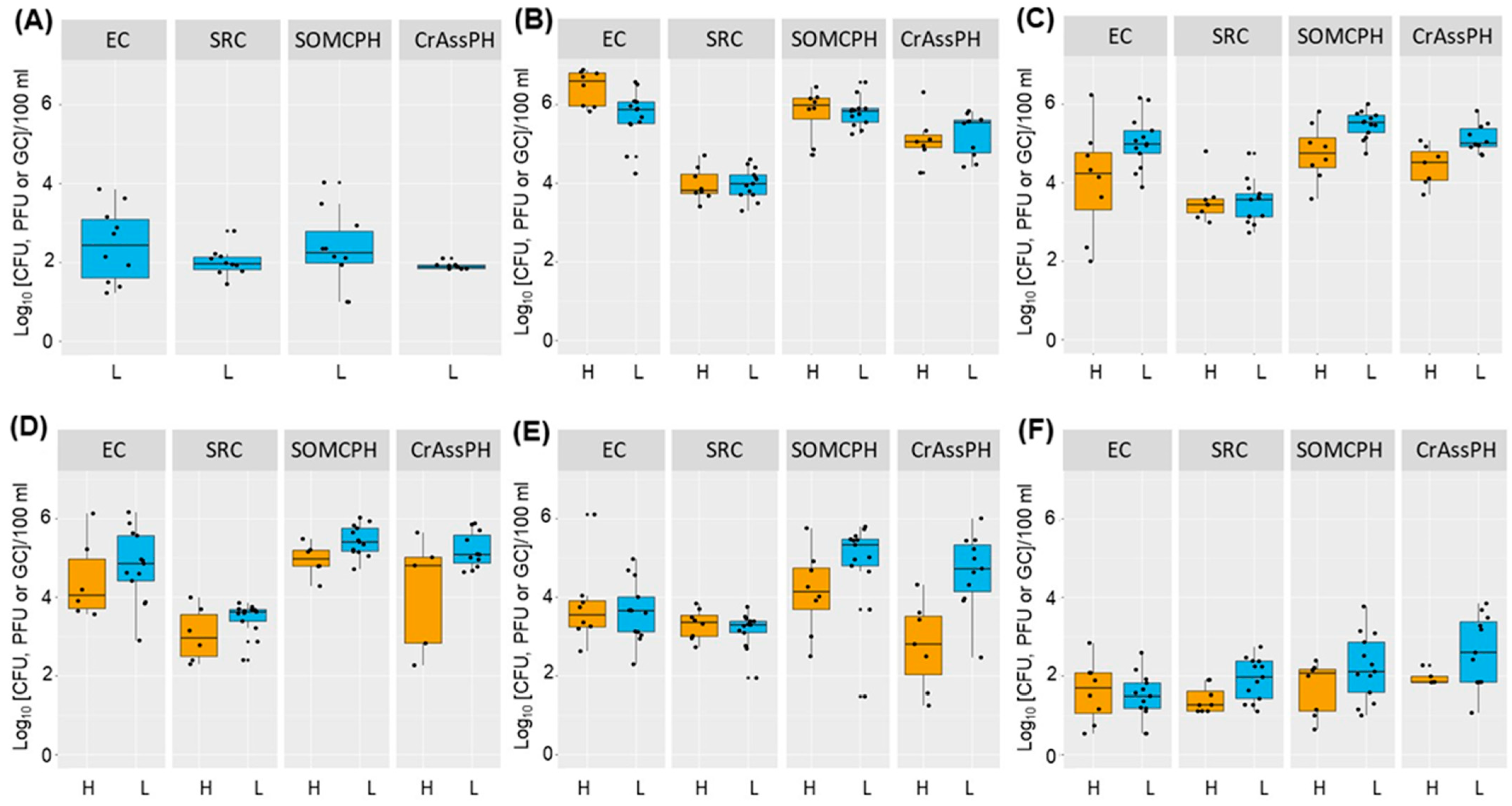
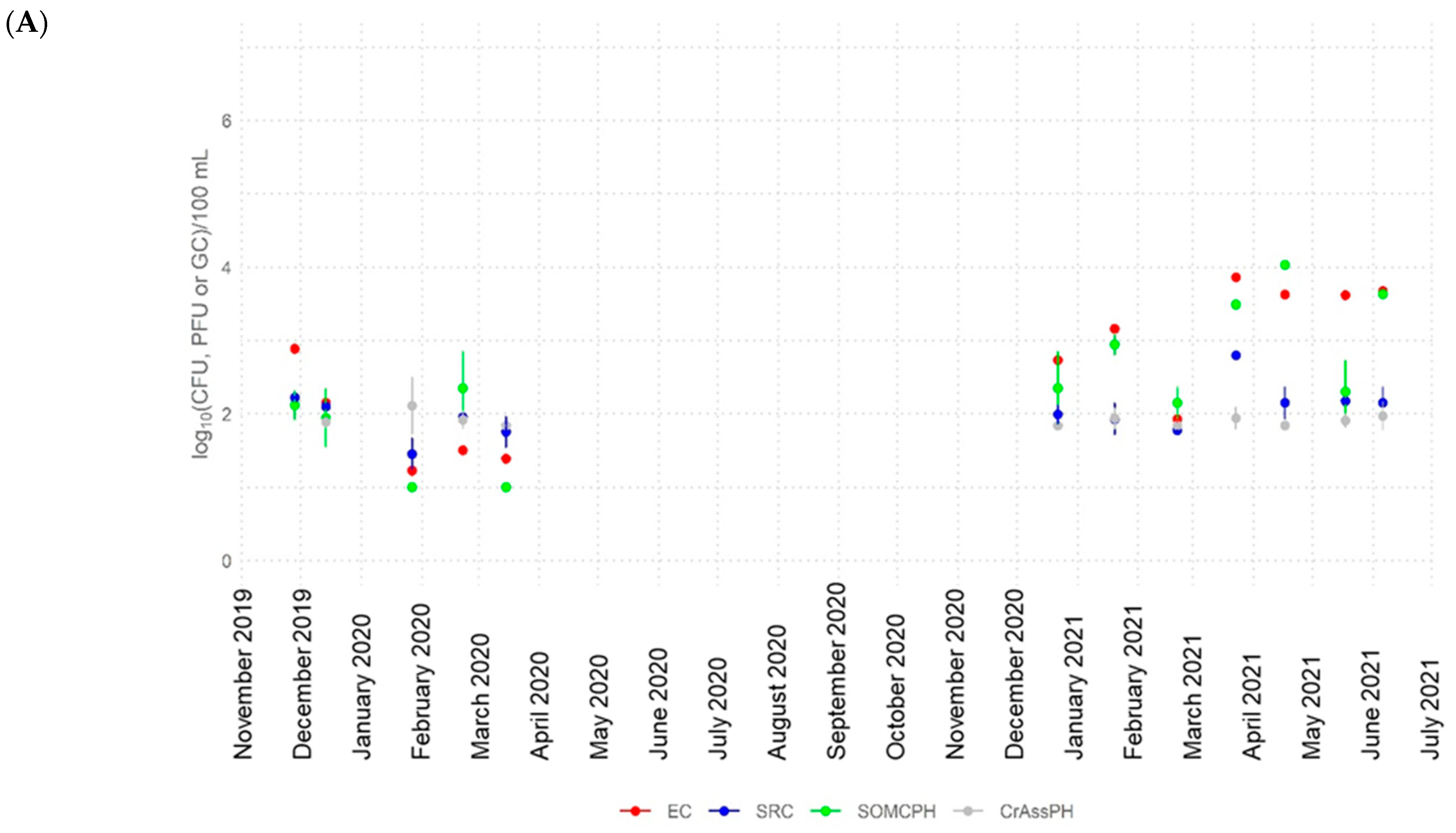
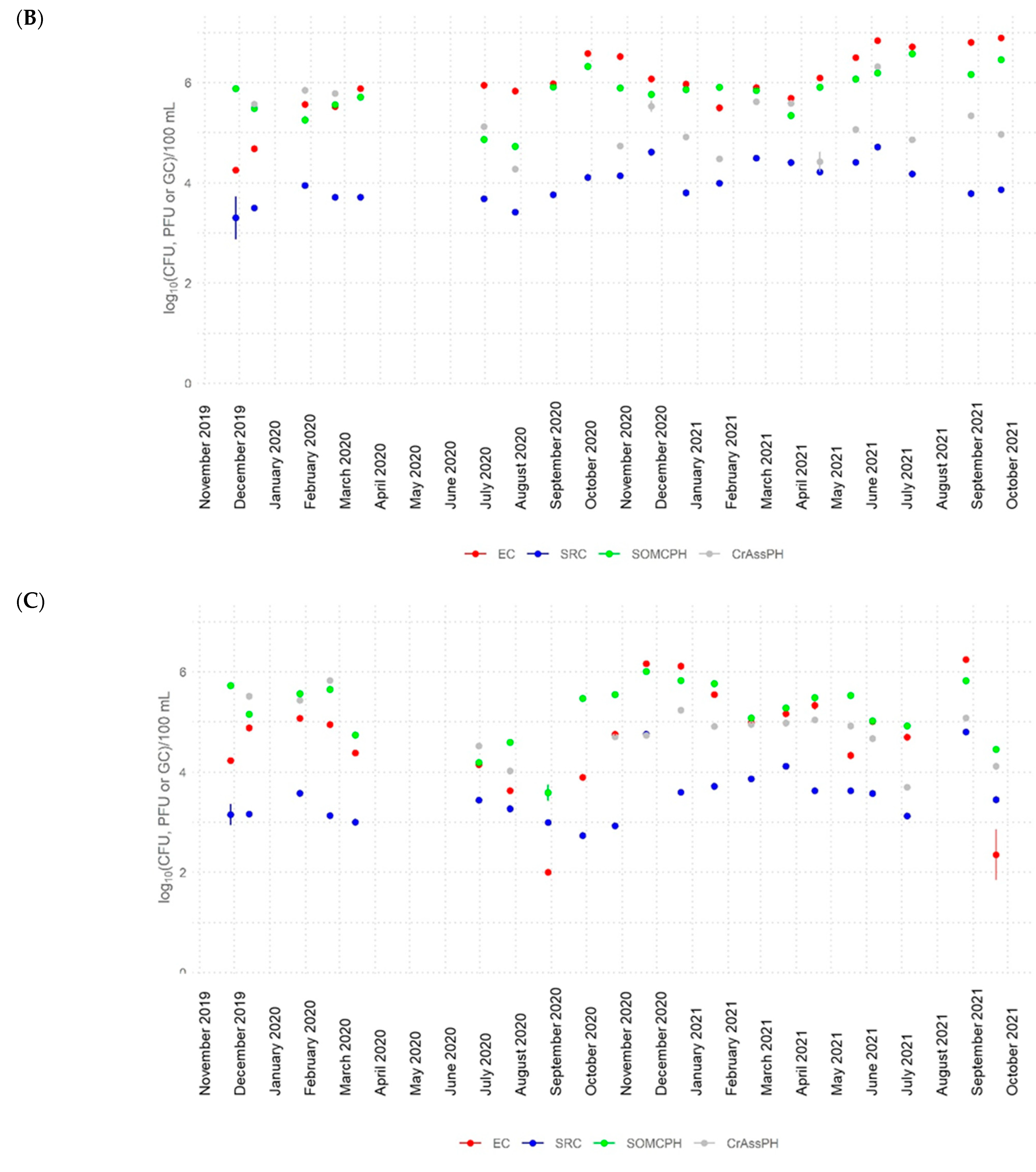
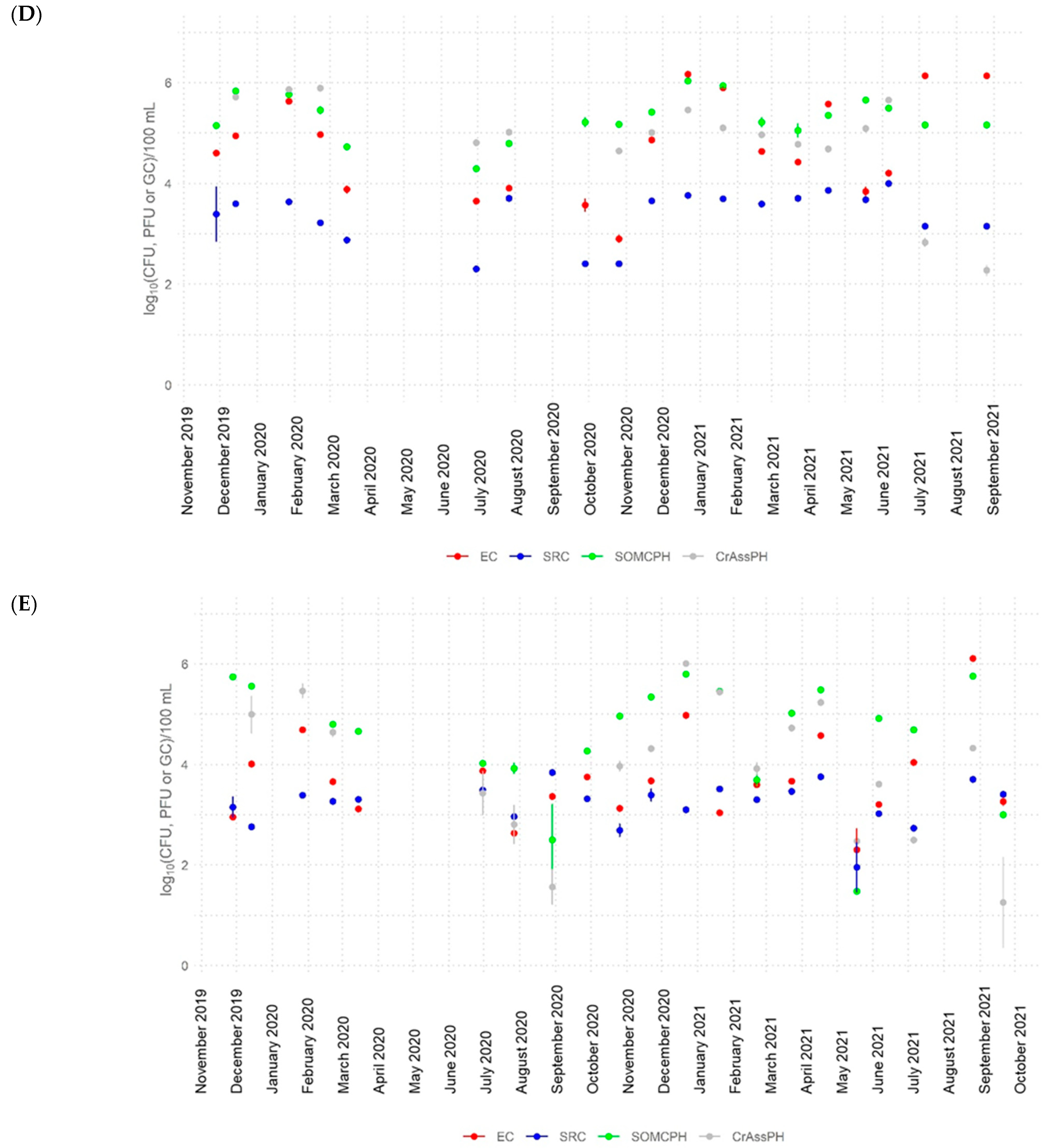
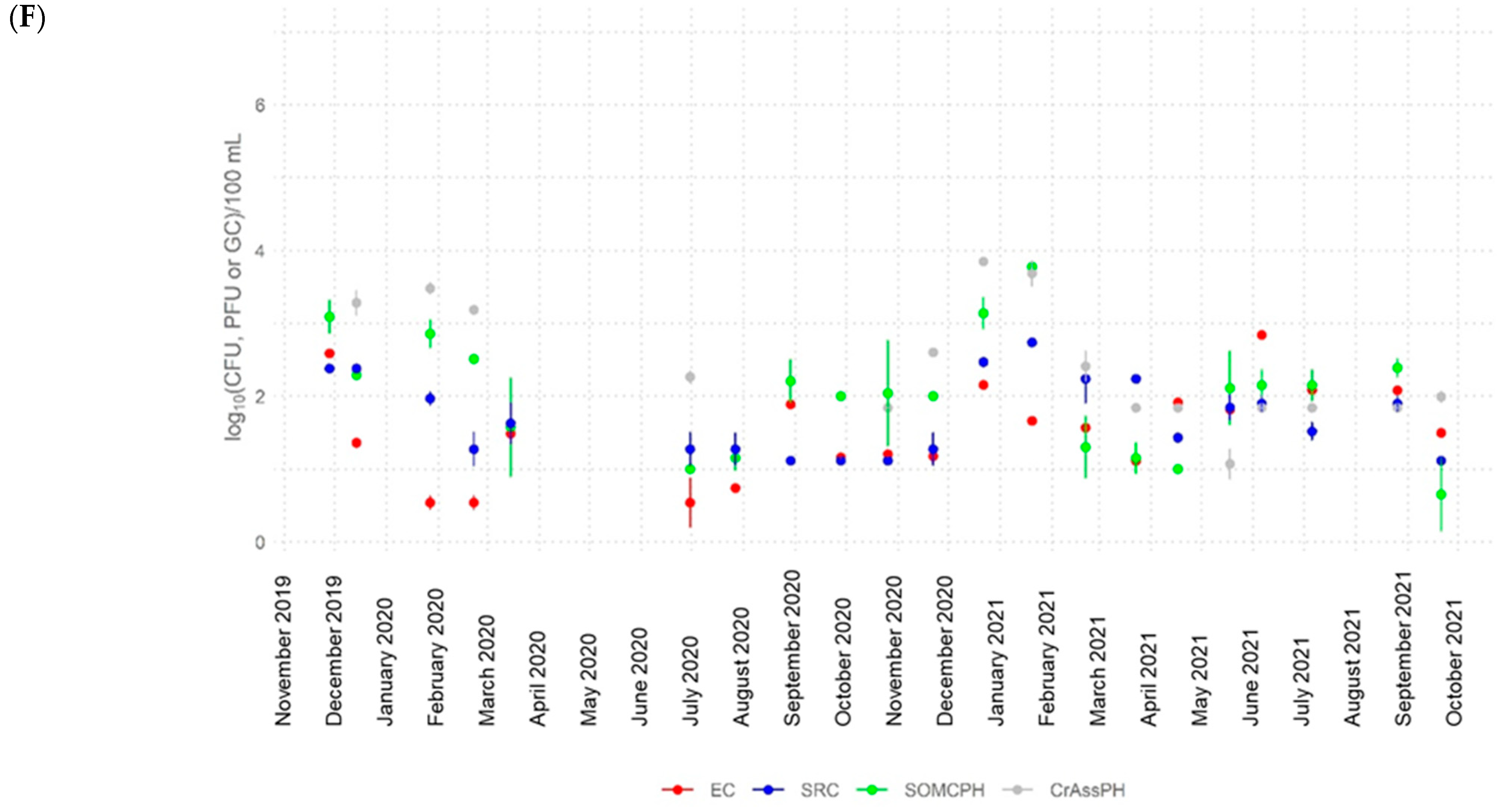
3.2. Dynamics of Fecal Indicators along the River

In general, no differences were observed between the first and second year of study for the different indicators, in the different sites, with the exception of S1, as described below. Nonetheless, seasonal differences were observed for certain indicators in diverse sites. A temporal graph of the microbial indicators across the different sites is shown in Appendix A (Figure A1).
During the first year of the study, samples at S1 exhibited low concentrations of fecal indicators, with mean concentrations of 2.1 ± 0.7 log10 CFU 100 mL−1 for EC, 2.0 ± 0.7 log10 PFU 100 mL−1 for SSRC, 1.9 ± 0.2 log10 CFU 100 mL−1 for SOMCPH, and 1.9 ± 0.1 log10 for CrAssPH (Figure 2A). However, during the second year of the study, there was a statistically significant increase of up to 1.5 log10 units in the concentrations of EC and SOMCPH and 0.4 log10 units for SSRC compared to the same period in the previous year (p < 0.05). At the end of the second year, there was a settlement of a small rural community near this sampling site, around 2000 inhabitants, and therefore, an additional fecal pollution input, resulting from the building of many farms to raise cows, sheep, and especially poultry, could explain this increase. In the case of CrAssPH, no significant increase was observed, which could be attributed to the fact that four of the samples were below the limit of detection for this marker before the construction of the community, which may have biased the comparison (Appendix A, Figure A2). At this site, no seasonal differences were observed since the water flow was null during the summer months.
The low levels of Indicators detected at this site are consistent with low levels of fecal pollution in the river. This site is formed by the convergence of two valleys: Wadi Gassar, which runs along the southern flank of Jebel Megress (altitude, 1737 m) and Wadi Ouricia, situated in the southern part of this mountain range. This fecal pollution could originate from human diffuse pollution as well as wildlife and farming activities, which may account for the higher levels of EC and SOMCPH with respect to CrAssPH, which has been reported as a potential human source tracking marker [47]. The concentrations of these indicators are similar to those reported in previous works for similar streams [48,49,50].
At S2, following the discharge of effluent from the Sétif WWTP, fecal indicators reached their highest concentrations, increasing by up to 4 log10 units. The mean concentration was 6.0 ± 0.7 log10 (CFU or PFU) 100 mL−1 for EC and SOMCPH, respectively. CrAssPH was detected at a mean concentration of 5.2 ± 0.6 log10 GC 100 mL−1, while SSRC levels were 4 ± 0.4 log10 CFU 100 mL−1 (Figure 2B). A statistically significant difference was observed between the high-temperature vs. low-temperature samples for EC, with mean concentrations of 6.6 and 5.6 log10 CFU 100 mL−1, respectively (p < 0.05), while no significant differences were observed for the other indicators.
We did not have access to the Sétif WWTP to know the efficiency of the treatment plant, but raw sewage levels of fecal indicators in another WWTP in a close area showed the following levels of fecal indicators: 7.1 log10 100 mL−1 for EC, 6.8 log10 100 mL−1 for SOMCPH, 7.5 log10 100 mL−1 for CrAssPH, and 4.9 log10 100 mL−1 for SSRC (personal data), which are highly similar to those observed at S2, indicating that the WWTP was not working efficiently. The observed levels of EC and SSRC in sewage were similar to those reported previously in other countries such as South Africa [51], India [52,53,54], or Algeria [55]. In the case of SOMCPH, the values were similar to those reported in other countries such as South Africa [56], Tunisia [57], and several European countries [58]. For CrAssPH, the sewage values were around one and two log10 lower than those reported in UK [59] or in Tampa, Florida [29], but in the same range as those reported in Spain [23]. Differences among the different countries can be attributed to different CrAssPH targets and used methods as well as different abundances of crAss-like phages in the different human populations [60].
At S3, there was a decrease in the levels of fecal indicators (approximately 20 km downstream of S2). This decrease was much higher at high temperatures, with the exception of SSRC, for which no seasonal differences were observed. Specifically, a reduction of 2.4 log10 was observed for EC, of 1.0 log10 for SOMCPH, of 0.4 log10 for SSRC, and of 0.7 log10 for CrAssPH when the temperature was high (p < 0.05). In the low-temperature group, there was a decrease of 0.7 log10 for EC, of 0.3 log10 for SOMCPH, and of 0.5 log10 for SSRC (p < 0.05). No differences were observed for CrAssPH at low temperatures between S2 and S3 although statistically significant seasonal differences were observed at this site.
In the tributary river (S4), the concentrations of fecal indicators were similar to the concentrations found in S3 (Figure 2D), indicating that the tributary river also contained high levels of urban fecal pollution, since crAssphage was also present at high levels.
The levels of fecal indicators at S5 (six km downstream of S3) were lower compared to those at S3 and S4. At this site, the mean concentrations were 3.7 ± 0.9 log10 CFU 100 mL−1 for EC, 4.6 ± 1.2 log10 PFU 100 mL−1 for SOMCPH, and 3.2 ± 0.4 log10 CFU 100 mL−1 for SSRC. The concentration of CrAssPH was 3.9 ± 1.4 log10 GC 100 mL−1 (Figure 2E). Seasonal differences in the concentrations were detected again for SOMCPH and CrAssPH between the high- and low-temperature groups (p < 0.05). If we take a look at the reductions from S3 to S5, different trends are observed depending on the indicators. Specifically, there was a higher decrease of EC at low temperatures, while in the cases of SOMCPH and CrAssPH, the opposite was observed.
Finally, there was a decrease in all the fecal indicators at S6, the water reservoir that was used for water production by a drinking water treatment plant. The mean concentration of the fecal indicators ranged between 1.5 log10 CFU 100 mL−1 for EC and 2.0 log10 PFU 100 mL−1 for SOMCPH, with SSRC levels at 1.7 log10 CFU 100 mL−1. The concentration of CrAssPH was slightly higher, 2.4 log10 GC 100 mL−1, although 13 out of 21 samples were below the limit of detection (Figure 2F). Once again, the concentrations of the different indicators were lower at high temperatures, although this was statistically significant only for SSRC. Compared to S5 (~9.5 km upstream), there were global reductions of 2.2 log10 units for EC, 2.6 log10 units for SOMCPH, and 1.5 log10 units for both SSRC and CrAssPH. Overall, there were reductions of more than 4 log10 for EC and SOMCPH, more than 3 log10 for CrAssPH, and more than 2 log10 for SSRC throughout a water flow distance of more than 30 km from the WWTP effluent discharge to the water reservoir.
The fecal pollution was subjected to natural inactivation downstream, as well as a removal of the water column through sedimentation processes and dilution from other tributaries such as the River El Mellah, until reaching the water reservoir, where it was highly diluted. The River Boussellam has an average annual flow rate of 0.48 (m3/s). The reservoir currently stores a volume of water of 121.40 million m3, regulating a volume of 50 million m3/year, in order to ensure the needs of drinking and industrial water for the populations of the towns of Sétif, Bordj Bou Arreridj, El Eulma, and other municipalities.
The different indicators underwent different reductions, with EC being the one that was inactivated at a higher rate with a 1 log10 reduction for EC in a transect of 6 km (from S3 to S5), followed by 0.9 log10 for CrAssPH and 0.6 log10 for SOMCPH. Finally, the most resistant was SSRC, which was reduced only by 0.3 log10 within this transect. This is consistent with the fact that EC has been reported as a non-conservative indicator, whereas SOMCPH has been reported as a semiconservative parameter, and SSRC as a conservative parameter [61]. In the case of the molecular marker CrassPH, the decay rate seems to be similar to that of SOMCPH [25]. Quantitative PCR is a rapid molecular technique that provides reliable results in less than one hour. Different qPCR methods have been approved by the EPA, such as US EPA Method 1609 for Enterococci and the EPA Method 1696 for the human microbial source tracking marker HF183 [62,63], and used for water remediation monitoring, but none have been approved to date for crAssphage.
Seasonal differences were observed in the concentrations and persistence of the different indicators and CrAssPH at some of the sites and along the distance. While it was not possible to assess the effect of temperature at S1, since it was dry during the summer period, the higher and statistically significant decrease observed for SOMCPH and CrAssPH between S3 and S5 in the high-temperature period vs. the low-temperature period is consistent with previous studies [50]. Nevertheless, in the case of EC, the lower amount of decrease observed during the high-temperature period between both sites could be attributed to a possible regrowth of EC during the high-temperature period at this site or a diffuse of animal pollution or a combination of both. At S5, agricultural activities, such as the use of animal feces as fertilizer during this season may have led to an increase in EC levels in the water. The river is an important water source for grazing sheep and cows on the banks, especially in the summer and in a semi-arid region such as Sétif. Previous reports have indicated EC regrowth in certain regions where warm climate and organic material are present [64]. In general, EC survive for 4 to 12 weeks in water at a temperature of 15–18 °C [65], and according to the research conducted by Ishii, the frequency of EC is higher from July to September due to more favorable temperatures [66]. SOMCPH is very unlikely to replicate in the environment [67]. In the same line, CrassPH is not expected to replicate in the environment since its host, Bacteroides, is anaerobic [19].

3.3. Correlation between the Fecal Indicators and CrAssPH

The co-occurrence of CrAssPH with the presence of fecal indicators was assessed by a study on pairwise correlations between the culturable indicators and CrAssPH. The culturable indicators EC, SOMCPH, and SSRC exhibited the highest correlations among them, moderate to very strong correlations at S1, S2 and S3 (Table 1), whereas in more aged, polluted waters, their correlation was less evident. On the other hand, the CrAssPH marker showed the highest correlation coefficients, with SOMCPH ranging from 0.50 to 0.88 at S3, S4, S5, and S6 (Table 1). The correlation of different crAssphage targets and fecal indicators has been previously reported in different water environments showing different correlation coefficients with SOMCPH as well as with human enteric viruses in wastewaters [26,27,59,68], sludge [69], and other fecal polluted waters [25,30,31,69,70].
Correlation is greatly affected by the methodology used [71]. In this case, we were correlating a molecular marker quantified via qPCR against a culturable marker, or different culturable indicators analyzed using different methodology. This effect may be magnified in samples with low targets or samples with little variation such as the highly polluted waters of S2 in the case of CrAssPH. Previous studies have reported higher correlations between the concentrations of some indicators in river water near the wastewater treatment plant than further downstream or upstream [68,72,73,74,75,76,77,78,79] Our results, show a high correlation at a longer distance between SOMCPH and CrAssPH, suggesting that they are decaying at a similar rate, which is in accordance with previous results conducted in mesocosms with both indicators [25]. Nevertheless, the various correlations observed in the literature with the different CrAssPH targets highlight the need of performing more studies to understand their usefulness in different geographic regions.

3.4. Dynamics of Bacterial Communities along the River

The assessment of the spatio-temporal dynamics of bacterial communities is very important for understanding the diversity, structure, and function of the river ecosystem that drains into the reservoir. One of the major advantages of using targeted metagenomic techniques, such as 16S rRNA gene sequencing, is that they are culture independent and can theoretically recover almost all bacterial taxa in any habitat.

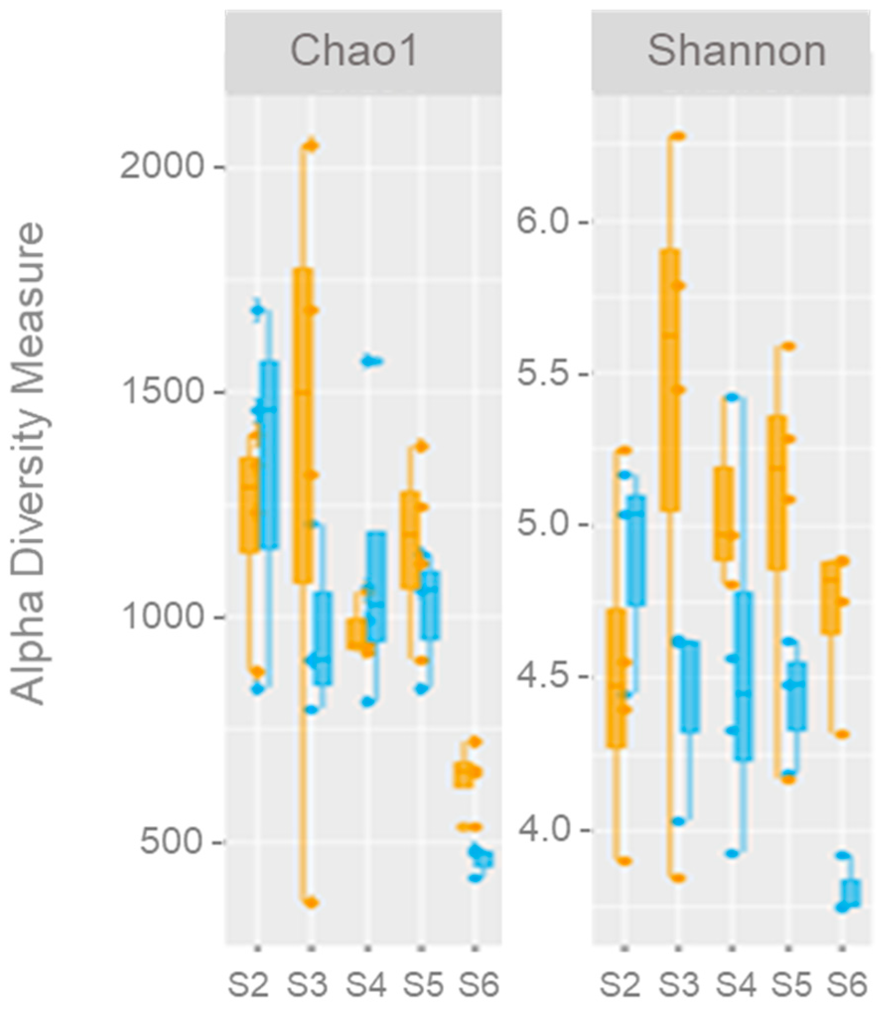
3.4.1. General Microbial Diversity

A total of 6,800,310 reads were obtained from the 33 sequenced samples. Samples from S1 exhibited a low number of reads (<3000 reads per sample). Despite the insufficient depth for a comprehensive description of the S1 communities, two samples with the highest number of non-chimeric filtered reads (801 and 601) were retained for a partial description of the community. The number of reads in all the negative controls (n = 3) ranged from 0 to 7. A summary of the data is provided in Appendix A (Table A3). The mean number of reads for the remaining samples generally exceeded 100,000 reads (185,830 ± 35,463 for site 2, 143,315 ± 55,606 for site 3, 165,947 ± 59,010 for site 4, 121,273 ± 54,455 for site 5, and 184,784 ± 39,768 for site 6). Rarefaction curves are shown in Appendix A (Figure A3). The majority of the reads were affiliated with Bacteria, with a minor proportion (<0.05%) being identified as Archaea. Subsequent analyses were performed only with Bacteria reads. The number of ASVs in each sampling site is shown in Table 2.

3.4.2. Bacterial Diversity

The diversity of bacterial communities was investigated in all sites, except for S1 due to the low coverage, following the rarefaction of the reads to the minimum value (43,009). The alpha diversity of the samples was characterized by analyzing species richness with Chao1, as well as the Shannon diversity index. The results obtained are shown in Table 2. No statistically significant differences were observed between the different sampling sites, except for S6, which showed the lowest mean value for both indexes (563 and 4.3 for Chao1 and Shannon, respectively), compared to the higher values observed in the other sites (>1000 and >4.8, respectively). Seasonal differences were observed in the Shannon index, with varying trends depending on the sampling site (see Figure 3). While the index was lower at high temperatures for S2, the opposite trend was observed in the other sites, although the difference was statistically significant only for S6 (p < 0.05). Different trends have been observed in the literature with respect to the relationship between diversity and temperature. While a higher diversity was observed during the low-temperature period in a temporary Mediterranean stream [35], in the work of Besemer et al. [80], the opposite was observed, similarly to our results. Decreases in diversity indices downstream in impacted rivers have also been previously reported [81], which aligns with the trend observed in our results, although it did not reach statistical significance due to the limited number of samples. In any case, the high bacterial diversity values suggest a capacity for adaptation and resilience among microbial populations to the perturbance, which is important to take into account when dealing with anthropogenic impacts within the global warming scenario.
The Bray–Curtis beta diversity index was used to assess the similarity of the bacterial populations present in the different sampling sites. The clustering of the samples based on this index showed two main clusters separating samples from S6 from the remaining samples and subclusters according to the sampling occasion and the temperature (Figure 4).
A non-linear multidimensional scaling (NMDS) representation of the Bray–Curtis index is shown in Figure 5. The NMDS1 component allowed the differentiation of samples from S6 from the remaining samples, while NMDS2 allowed the separation of the samples of high temperatures (upper part of the graph) and samples from the wet period with water flow in S1 (lower part of the graph). This differentiation was statistically supported through PERMANOVA (p < 0.05). Statistically significant SVs (p < 0.05) included, among others, SV3, which enabled the separation of S6 samples. This SV, affiliated to the Cyanobacteria genus Planktothrix NIVA-CYA 15, contributed approximately 10% of the observed differences.

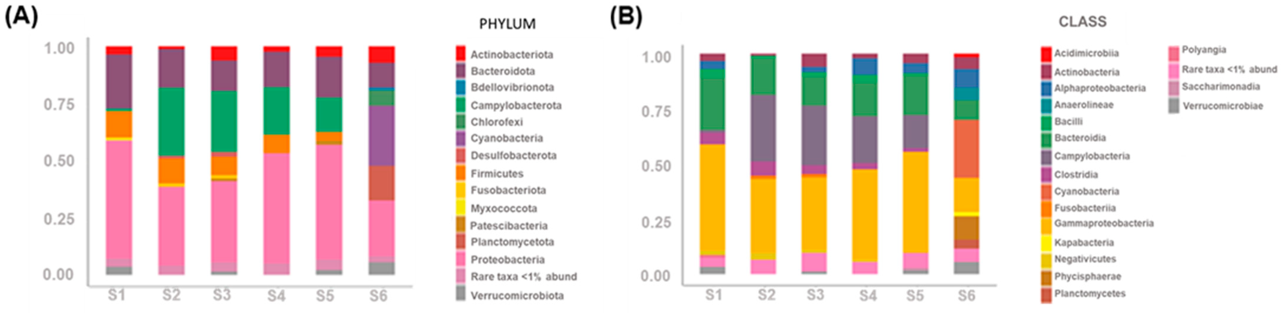
3.4.3. Bacterial Communities’ Taxonomy

For taxonomy, the identification of sequence variants (SVs) was conducted using the SILVA v138 database. It should be noted that certain taxa have been updated, such as Proteobacteria phylum, which has been reassigned under the Pseudomonadota phylum according to [82]. Nevertheless, we maintained the nomenclature of the database to facilitate comparison with previous studies.
The dominant phylum varied across sampling sites (Figure 6A). In S1, Proteobacteria (55.6 ± 17.7%) and Bacteroidota (23.0 ± 4.2%) were predominant, while in S2, Proteobacteria (34.6 ± 12.8%) and Campylobacterota (31.0 ± 15.8%) dominated. The third most dominant phylum was Bacteroidota (16.1 ± 5%). Proteobacteria continued to be the dominant phylum in subsequent sampling sites along the river, with mean relative abundances of 37.7%, 49.4%, and 52.6%, at S3, S4, and S5, respectively, while Campylobacterota decreased to around 20% in S3 and S4 and 10% in S5. Bacteroidota remained the third most abundant phylum in these sites. In the water reservoir (S6), the dominant phyla were Cyanobacteria (26.9 ± 15.3%), Proteobacteria (24.6 ± 10.6%), Planctomycetota (14.1 ± 6.2)%, Bacteroidota (12.8 ± 3.0%), and Chloroflexi (6.9 ± 3.6%). Cyanobacteria, Planctomycetota, and Chloroflexi accounted for approximately 50% of all the SVs in all reservoir samples. These findings are consistent with other studies, suggesting the dominance of the first two phyla in rivers and reservoirs [83,84] and suggesting a high versatility and capability of persisting in different environmental conditions.
Class Gammaproteobacteria (52.9 ± 21.7%) and Bacteroidia (22.6 ± 0.0%) were the most abundant in S1. In S2–S4, the top three classes were Gammaproteobacteria, Campylobacteria, and Bacteroidia, representing ~75% of the SVs, although changing in proportions along the river transect. Campylobacteria decreased, whereas Gammaproteobacteria increased, and Bacteroidia remained in the same range. In S6, class Cyanobacteria was dominant (26 ± 15%), followed by Gammaproteobacteria (15.8 ± 5.9%) and Phycisphaerae (9.8 ± 6.4%) (Figure 6B). This structure was maintained throughout the year independently of the season.
As expected from beta diversity results, the community structure at the genus level was similar among all the sites in the river sites with high levels of pollution. In taking all the samples together, the most prevalent genera were as follows: S1 was dominated by Sphaerotilus (47%) in one sample, followed by Prevotella (11 ± 5.6%), Massilia (9 ± 0.0%), and Rhodoferax (8.5 ± 2.1%), and Flavobacterium at a relative abundance of 9% was present in only one sample; S2, Arcobacter (23.6 ± 14.9%), Acinetobacter (8.5 ± 0.7%), Prevotella (6.2 ± 4.1%), and Pseudoarcobacter (4.6 ± 2.2%); S3, Arcobacter (16.4 ± 13.7%), Pseudoarcobacter (3.7 ± 4.0%), Aeromonas (3.4 ± 5.7%), and Polynucleobacter (2.9 ± 5.2%); S4, Arcobacter (13.4 ± 16.3%), Flavobacterium (6.5 ± 5.0%), and Hydrogenophaga (6.2 ± 7.0%); S5, Arcobacter (8.5 ± 12%), unassigned genus from Family Neisseriaceae (5.3 ± 11%), and Flavobacterium (5.1 ± 5.7%); and S6 was dominated by Planktothrix NIVA-CYA 15 (23.6 ± 14.3%), followed by genus CL500-3 from the family Phycisphaeraceae (7.8 ± 4.4%), an unassigned genus from family Caldilineaceae (5.7 ± 2.9%), and an unassigned genus from the SAR11 Clade III (3.7 ± 5.5%). More detailed information can be found in Supplementary Materials (krona html file).
The dominant genera observed in our work are in agreement with those in previous works, including the detection of genera Sphaerotilus, Prevotella, Massilia, or Rhodoferax in water environments with low levels of pollution, and Flavobacterium, Arcobacter, and Polynucleobacter in water samples containing high levels of fecal pollution [35]. Cianobacterial genus Planktothrix and members of the Phycisphaeraceae and Caldilineaceae families as well as members of SAR11 Clade III have been previously identified in freshwater systems [85].
When examining the shared SVs among samples from the same sampling sites, notable differences were observed. The sampling site with the highest number of shared SVs was S2, accounting for approximately 8% of shared SVs, followed by S6 with 5%. In contrast, S3, S4, and S5 exhibited much lower levels of shared sequences, ranging from 0.5% to 1% (Table 2, core SVs), indicating greater variability in these sites.
Some of this variability may be attributed to differences in SV distribution among samples based on the period of the year during which sampling occurred. This variability is evident in the heatmap representation of the 50 most abundant core SVs for each sampling site (see Figure 7). For instance, SV29, SV65, and SV78, affiliated with an unassigned genus of the family Neisseriaceae, genus Simplicispira, and genus Poseidonibacter, respectively, were not detected during the high-temperature period. SV124, affiliated with Rhodoferax, was not detected during the high-temperature period in S2 and S6 and detected in only one sample each from S3, S4, and S5 during the same period. SV151, affiliated to genus Hydrogenofaga, and SV11, affiliated to Aeromonas, were detected only during the high-temperature period in S6. These findings are consistent with the existence of representatives of these genera that are thermophilic phototrophs, especially in hot spring conditions [86,87,88]. SV1, affiliated to genus Arcobacter, was not detected during the high-temperature period in S6.
Bacteria play indispensable roles in various biogeochemical processes and pollutant degradation, and they can be useful in assessing the health of the aquatic ecological environment [89,90]. We did not analyze the impact of nutrient pollution on the bacterial communities, but there was a gradient in the nutrient content (PO43− and NH4+) from the most polluted sites to the less polluted sites. This gradient may have impacted the observed shifts in the bacterial communities, but the low numbers of sequenced samples were not sufficient to draw conclusions.

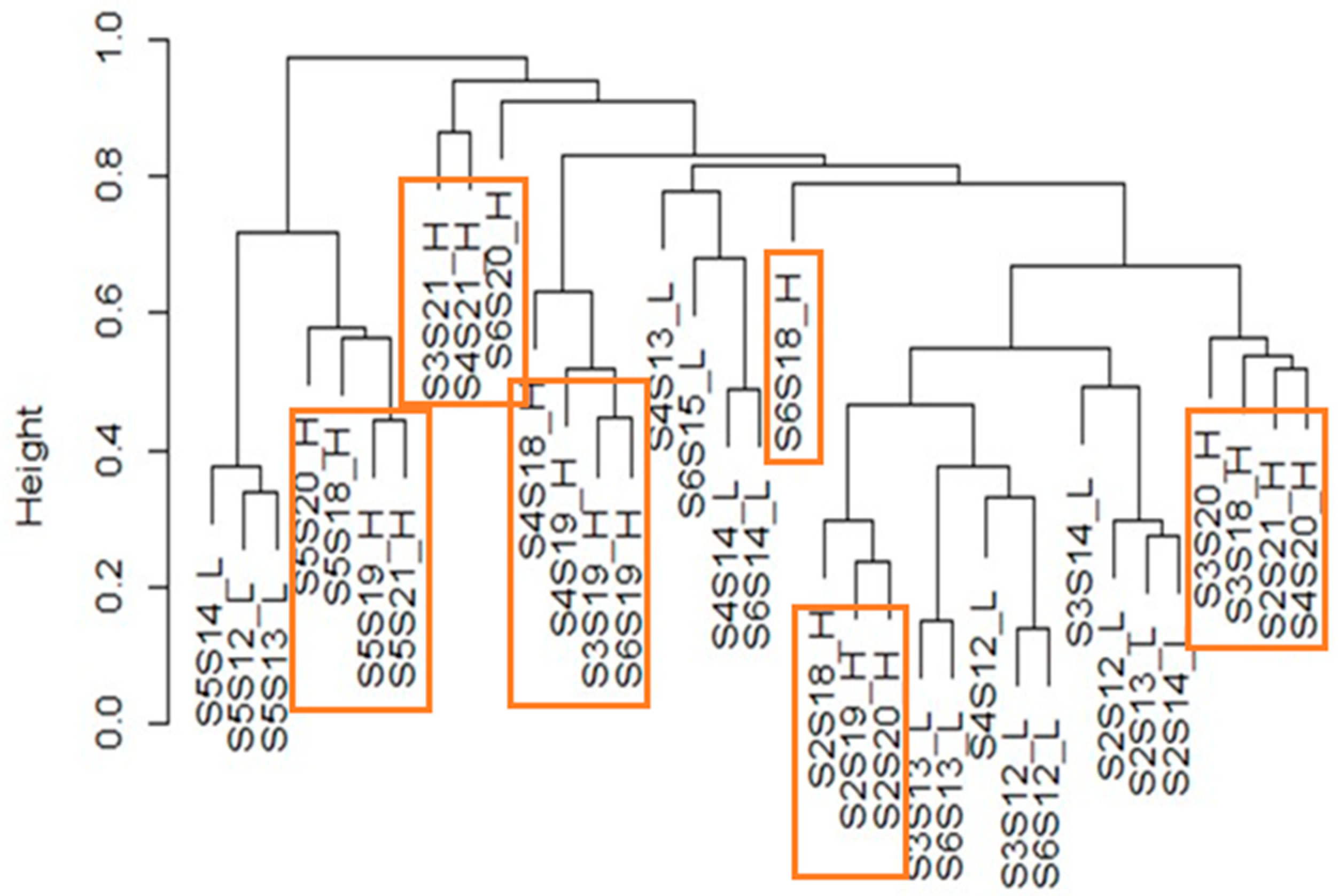
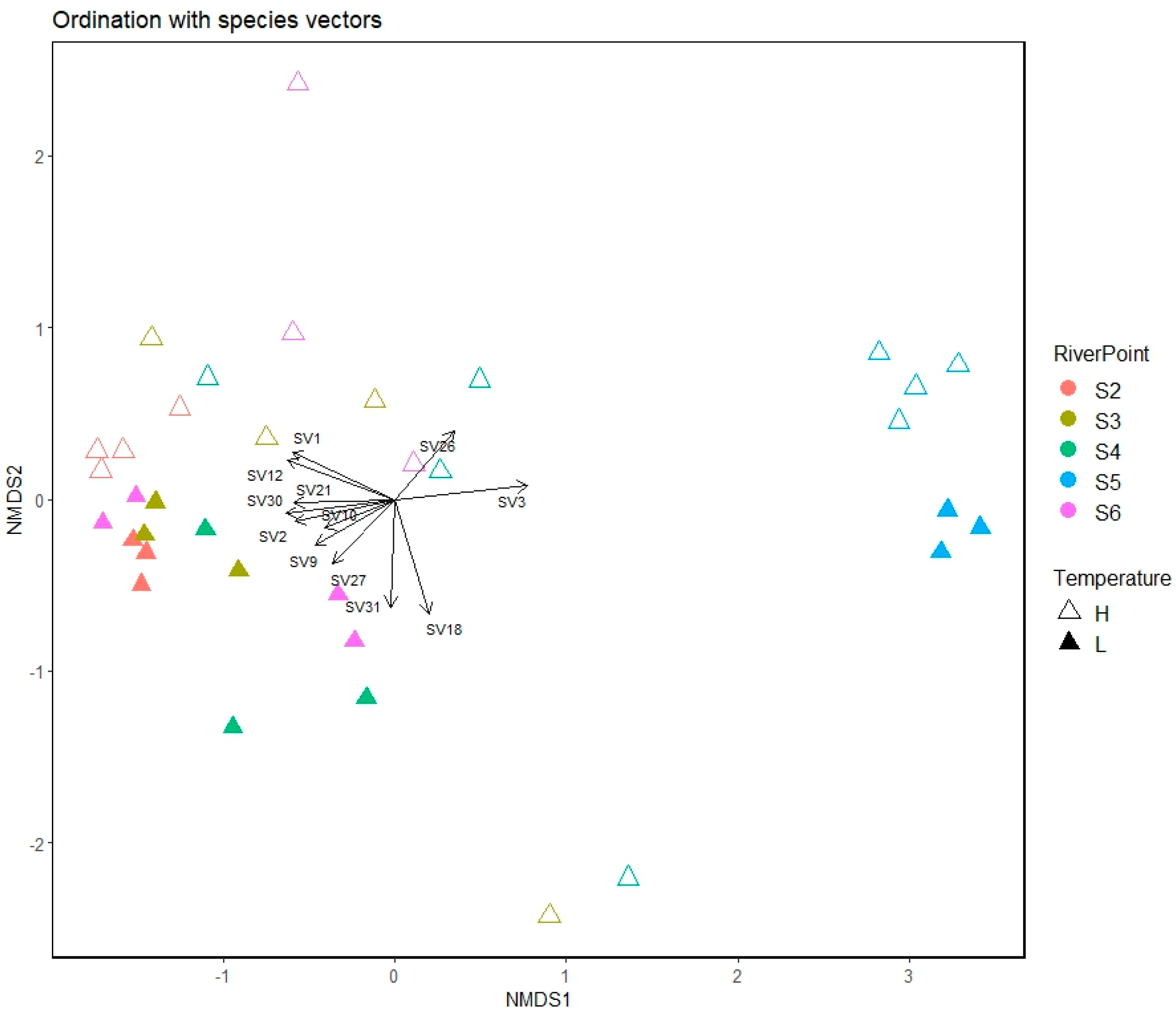
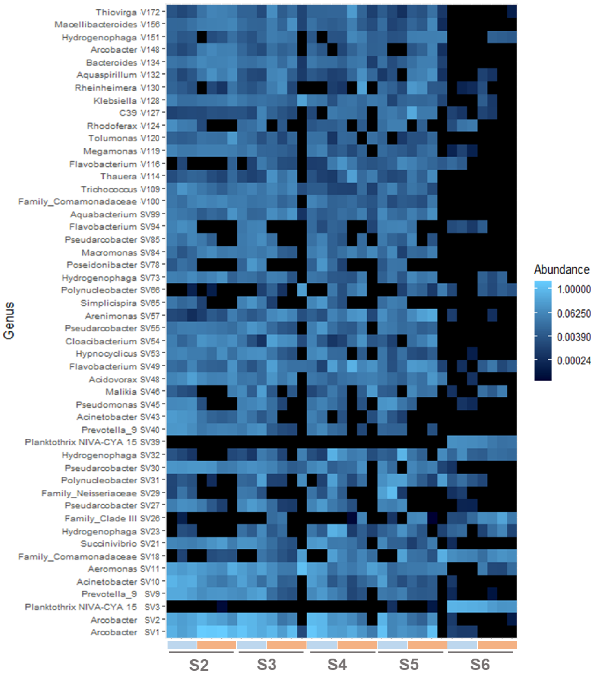
3.4.4. Tracking the ASVs along the Water Course

The Source Tracker algorithm was applied to elucidate the environmental influences on communities downstream of the river. When considering S3 as a sink, the reads tracked to originate from S2 or S4 were higher during the low-temperature period compared to the high-temperature period (p < 0.05), with a notable proportion of reads classified as of “unknown” origin (Table 3). When the S6 was used as a sink, more than 90% of the reads were classified as of “unknown” origin (Appendix A, Table A5). These results corroborate the spatial and temporal shift in the bacterial populations.
The high number of sequences assigned to “unknown origin” using the source tracker algorithm during the high-temperature period could be related to the fact that warm environmental conditions may facilitate microbial growth, which could also explain the greater diversity of microbial taxa during the analyzed period. For example, soil microbiomes may vary seasonally due to changes in temperature, leading to differences in the microbial communities. Therefore, the microbial communities in the samples during the dry period may be more diverse or influenced by other factors. Further investigation into the specific sources contributing to these “unknown” sequences may help elucidate the underlying reasons for these seasonal differences. On the other hand, at S6, the fact that less than 10% of the sequences could be tracked to a known origin is not strange since S6 is the most distant sampling site and was also the most distant in terms of community structure composition as revealed by NMDs. This may be the result of complex interactions between environmental factors and the water ecosystem along the water course, and completely different dynamics in the reservoir such as stratification and non-flowing waters. Understanding these factors is essential for managing and preserving water quality in freshwater ecosystems.

4. Conclusions

This study contributes the following:
  • This study presented data on the prevalence and abundance of crAssphage in environmental waters in Algeria for the first time.
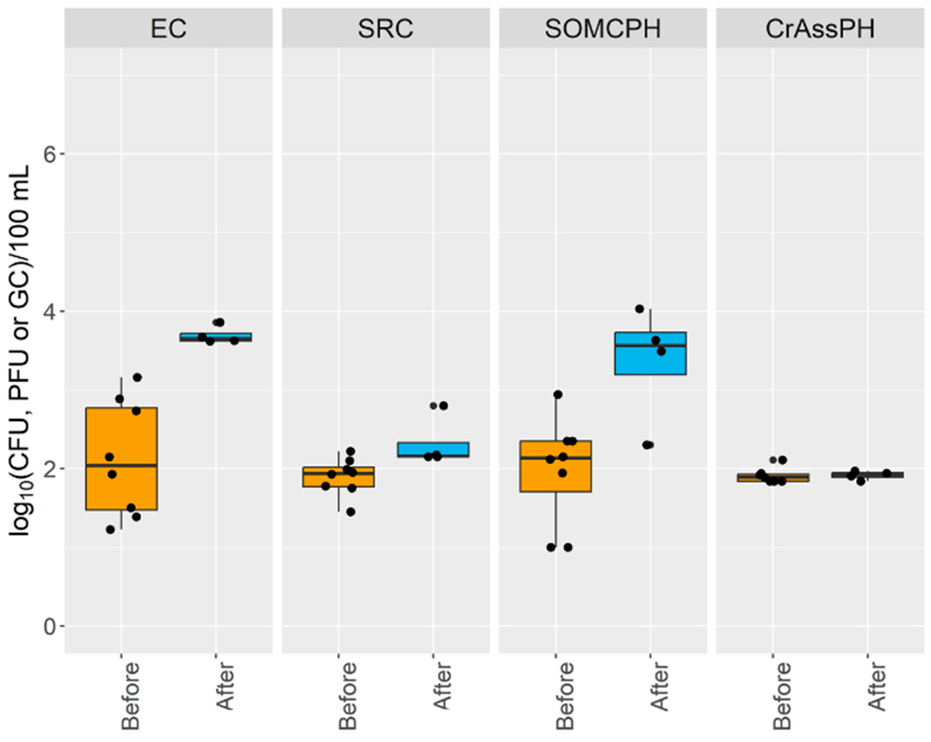
  • CrAssphage was frequently detected in river water at all sites (>5 log10 GC/100 mL at the most polluted site) and in the water reservoir at similar abundance values to other fecal indicators, showing strong correlations with somatic coliphages in the river (rho up to 0.88), with the signal fluctuating to lower levels along the river. These findings support the application of crAssphage as a human fecal pollution indicator for aged pollution in Algeria because of its high concentrations and persistence in the environment.
  • The high-temperature season produced a higher decrease in the numbers of the fecal indicators (>4 log10 for E. coli and somatic coliphages and >3 log10 for crAssphage). During this season, the bacterial communities in the river also varied, becoming more diverse.
  • The self-depuration capacity of the river reduced the impact of municipal wastewater from a microbiological point of view along its water course, as evidenced by the decrease in the number of fecal indicators, as well as crAssphage levels, to almost undetectable levels in the water reservoir. This self-purification was more pronounced during the high-temperature season, except for E. coli at site 5, where possible regrowth or contamination with animal fecal matter was detected.
  • The high bacterial diversity values during the high-temperature period suggest a capacity for adaptation and resilience among microbial populations to disturbances, which should be considered when addressing anthropogenic impacts within the context of global warming.
  • In summary, this study provides valuable insights into the complex interplay between anthropogenic activities, wastewater discharge, and microbial pollution in a highly urban-impacted watershed in Algeria, where limited information is available. The irrigation of crops with the river water, especially in the near highly populated areas, as a common practice in the region, poses a risk for the transmission of fecal-oral pathogens to the population. The continued monitoring and implementation of appropriate management measures are essential to safeguard water quality and public health in these vulnerable environments.

Supplementary Materials

The following supporting information can be downloaded at: https://www.mdpi.com/article/10.3390/w16081123/s1, krona html file.

Author Contributions

Conceptualization, S.M.-A. and C.G.-A.; resources, all authors (D.B., A.B., E.B., S.M.-A. and C.G.-A.); writing—original draft preparation, D.B. and C.G.-A.; writing—review and editing, all authors (D.B., A.B., E.B., S.M.-A. and C.G.-A.); supervision, S.M.-A. and C.G.-A. All authors have read and agreed to the published version of the manuscript.

Funding

This research was funded by the EU, PRIMA, BENEFIT-Med, grant number: 1726; the Ministerio de Ciencia, Innovación y Universidades (MICIU), EPIC grant number: PID2020-113355GB-100; and BACTPLAST, grant number: PID2019-108957GA-I00; the AGAUR, 2021SGR01081; and the Institut de Recerca de l’Aigua de la Universitat de Barcelona.

Data Availability Statement

Data are available upon request. Sequencing data are available from the Mendely Data public repository (https://data.mendeley.com/drafts/5knb8bsk28, accessed on 30 March 2024).

Acknowledgments

We would like to thank Joan Jofre for his helpful comments and review of the whole manuscript, and the Bacteriological laboratory and the Molecular biology laboratory of the Anti-Cancer Center (CAC) of Sétif.

Conflicts of Interest

The authors declare no conflicts of interest. The funders had no role in the design of the study; in the collection, analyses, or interpretation of data; in the writing of the manuscript; or in the decision to publish the results.

Appendix A

Table A1. Meteorological data obtained from an automatic station close to the river during the sampling campaigns.
Sampling CampaignsSampling DatesSeasonRainRain B1T MinT MaxHumidityHumidity B1
1 28 November 2019A 0 0 6 15 81 74
2 14 December 2019W 0 0 6.1 15 75 73
3 27 January 2020W 2 0.3 1 10.2 73 82
4 22 February 2020W 0 0 −0.4 16 39 29
5 15 March 2020SP 0 0 5.3 19 67 67
6 30 June 2020S 0 0 19.7 36.2 19 22
7 27 July 2020S 0 0 24 38.2 24 19
8 29 August 2020S 0 0 22.4 33.2 21 30
9 28 September 2020A 0 0 5.9 22 33 35
10 26 October 2020A 0 0 5.3 19 52 49
11 22 November 2020A 3 9.9 5 9 91 85
12 22 December 2020W 5.3 15.6 2 12 86 88
13 20 January 2021W 0 0 −1.4 12 60 43
14 21 February 2021W 0 0 4.1 17.8 38 34
15 23 March 2021SP 5.1 4.1 1 8.5 85 78
16 17 April 2021SP 3.1 1 4.6 10 81 70
17 18 May 2021SP 0 0 13.9 28.3 36 43
18 06 June 2021S 1 0 15 23 46 61
19 06 July 2021S 0 0 23.5 40 15 17
20 26 August 2021S 3.1 7.1 17 31 42 48
21 21 September 2021A 1 28.1 15 25 59 69
Note: Rain: Rainfall on the sampling day (mm). Rain B1: Rainfall 1 day before the sampling day (mm). Season: winter (W), summer (S), Autumn (A), Spring (SP). T max: Maximum air temperature (°C). T min: Minimum air temperature (°C). Humidity: Humidity of the sampling day. Humidity B1: Humidity 1 day before the sampling day.
Table A2. Physico-chemical parameters of the water.
pH C
(µS/CM)
T
(NTU)
PO43− (mg/mL) NH4+ (mg/mL) NO2
(mg/mL)
OM
(mg/L)
Site 1 8.1 ± 0.3 953 ± 119 8.3 ± 10.5 1.6 ± 1.6 2.3 ± 3.6 0.2 ± 0.1 12.2 ± 6.1
Site 2 7.7 ± 0.3 1398 ± 224 38.0 ± 16.5 4.1 ± 2.3 6.9 ± 3.7 0.3 ± 0.2 19.7 ± 10.3
Site 3 7.9 ± 0.3 2275 ± 769 37.2 ± 9.5 4.3 ± 1.8 6.7 ± 2.5 1.1 ± 1.3 26.0 ± 21.1
Site 4 8.1 ± 0.5 3284 ± 1208 31.9 ± 20.7 5.3 ± 2.1 5.3 ± 2.1 1.1 ± 1.8 23.3 ± 19.4
Site 5 7.5 ± 0.6 3165 ± 1691 41.0 ± 46.8 2.0 ± 1.4 4.1 ± 3.4 0.6 ± 1.4 16.0 ± 10.7
Site 6 7.5 ± 0.6 1621 ± 73 32.2 ± 13.1 1.2 ± 1.2 2.4 ± 1.0 0.6 ± 0.5 21.2 ± 16.9
Note: Results are expressed as mean ± SD. T, turbidimetry; C, conductimetry; OM, organic matter.
Table A3. Summary of the sequencing results.
SampleNInputFiltereddenoisedFdenoisedRMergedNonchimeric
Site 12417832471938193214021402
Site 271,567,8371,431,8661,400,9221,404,5681,328,4411,300,807
Site 371,225,7851,117,8511,089,0821,091,0911,024,1331,003,202
Site 471,403,6531,273,2391,245,5681,249,1131,184,8751,161,627
Site 571,056,645954,990922,552924,741862,151848,908
Site 671,539,2801,381,8301,366,5071,367,4131,316,7901,293,487
Negative DNA ext #116954816866
Negative DNA ext #21824285100
Negative sequencing1427247777
Positive control1114,168103,850103,432103,651101,73598,655
Note: N, number of samples.
Table A4. Statistically significant SVs from the top 20 SVs that explained the ordination of the samples (p < 0.05).
SVPhylumClassOrderFamilyGenus
1CampylobacterotaCampylobacteriaCampylobacteralesArcobacteraceaeArcobacter
2CampylobacterotaCampylobacteriaCampylobacteralesArcobacteraceaeArcobacter
3CyanobacteriaCyanobacteriiaCyanobacterialesPhormidiaceaePlanktothrix
NIVA-CYA 15
9BacteroidotaBacteroidiaBacteroidalesPrevotellaceaePrevotella
10ProteobacteriaGammaproteobacteriaPseudomonadalesMoraxellaceaeAcinetobacter
11ProteobacteriaGammaproteobacteriaEnterobacteralesAeromonadaceaeAeromonas
12ProteobacteriaGammaproteobacteriaEnterobacteralesEnterobacteriaceaeEscherichia-Shigella
18ProteobacteriaGammaproteobacteriaBurkholderialesComamonadaceaeFamily_
Comamonadaceae
21ProteobacteriaGammaproteobacteriaEnterobacteralesSuccinivibrionaceaeSuccinivibrio
26ProteobacteriaAlphaproteobacteriaSAR11 cladeClade IIIFamily_Clade III
27CampylobacterotaCampylobacteriaCampylobacteralesArcobacteraceaePseudarcobacter
30CampylobacterotaCampylobacteriaCampylobacteralesArcobacteraceaePseudarcobacter
31ProteobacteriaGammaproteobacteriaBurkholderialesBurkholderiaceaePolynucleobacter
Table A5. Identification of source of reads using S6 as sink.
Sample Conditions S2 S3 S4S5Unknown
S6S12 L 0.00 ± 0.000.32 ± 0.320.76 ± 0.291.71 ± 0.5997.21 ± 0.46
S6S14 L 0.15 ± 0.100.20 ± 0.121.03 ± 0.212.14 ± 0.4296.50 ± 0.35
S6S13 L 0.07 ± 0.070.24 ± 0.170.27 ± 0.121.35 ± 0.4298.00 ± 0.50
S6S18 L 0.18 ± 0.151.15 ± 0.320.67 ± 0.321.89 ± 0.4196.11 ± 0.40
S6S19 H 0.21 ± 0.050.65 ± 0.311.55 ± 0.255.67 ± 0.5491.92 ± 0.54
S6S20 H 0.04 ± 0.160.6 ± 0.321.25 ± 0.342.9 ± 0.6695.22 ± 0.62
S6S21 H 0.01 ± 0.030.44 ± 0.140.49 ± 0.222.62 ± 0.2596.44 ± 0.41
Note: L, low temperature; H, high temperature. Mean values ± standard deviation. Possible origins: S2, S3, S4, and S5.
Figure A1. Dynamics of the culturable indicators and CrAssPH over the two years of study at Site 1 (A), Site 2 (B), Site 3 (C), Site 4 (D), Site 5 (E), and Site 6 (F). EC (E. coli), SRC (spores of sulfite-reducing clostridia), SOMCPH (somatic coliphages), CrAssPH (crAssphage).
Water 16 01123 g0a1aWater 16 01123 g0a1bWater 16 01123 g0a1cWater 16 01123 g0a1d
Figure A2. Impact of the construction of an urban community near sampling site 1 on the concentration of the fecal indicators. Their concentrations ‘before’ and ‘after’ the construction are shown. EC (E. coli), SRC (spores of sulfite-reducing clostridia), SOMCPH (somatic coliphages), CrAssPH (crAssphage).
Water 16 01123 g0a2
Figure A3. Rarefaction curves of the obtained reads for the different sampling sites.
Water 16 01123 g0a3

References

  1. Zittis, G.; Hadjinicolaou, P.; Klangidou, M.; Proestos, Y.; Lelieveld, J. A Multi-Model, Multi-Scenario, and Multi-Domain Analysis of Regional Climate Projections for the Mediterranean. Reg. Environ. Chang. 2019, 19, 2621–2635. [Google Scholar] [CrossRef]
  2. IPCC. Climate Change 2022: Impacts, Adaptation and Vulnerability; Pörtner, H.-O.D.C., Roberts, M., Tignor, E.S., Poloczanska, K., Mintenbeck, A., Alegría, M., Craig, S., Langsdorf, S., Löschke, V., Möller, A., et al., Eds.; Cambridge University Press: Cambridge, UK, 2022; ISBN 9789291691623. [Google Scholar]
  3. Mohammed, T.; Al-Amin, A.Q. Climate Change and Water Resources in Algeria: Vulnerability, Impact and Adaptation Strategy. Econ. Environ. Stud. 2018, 18, 411–429. [Google Scholar] [CrossRef]
  4. Khalid, S.; Shahid, M.; Natasha; Bibi, I.; Sarwar, T.; Shah, A.H.; Niazi, N.K. A Review of Environmental Contamination and Health Risk Assessment of Wastewater Use for Crop Irrigation with a Focus on Low and High-Income Countries. Int. J. Environ. Res. Public Health 2018, 15, 895. [Google Scholar] [CrossRef] [PubMed]
  5. Edberg, S.C.; Rice, E.W.; Karlin, R.J.; Allen, M.J. Escherichia Coli: The Best Biological Drinking Water Indicator for Public Health Protection. J. Appl. Microbiol. 2000, 88, 106S–116S. [Google Scholar] [CrossRef]
  6. Saingam, P.; Li, B.; Yan, T. Fecal Indicator Bacteria, Direct Pathogen Detection, and Microbial Community Analysis Provide Different Microbiological Water Quality Assessment of a Tropical Urban Marine Estuary. Water Res. 2020, 185, 116280. [Google Scholar] [CrossRef] [PubMed]
  7. NHMRC. Australian Drinking Water Guidelines Paper 6: National Water Quality Management Strategy, Version 3.4 Updated October 2017; NHMRC: Canberra, Australia, 2011; ISBN 1864965118. [Google Scholar]
  8. European Commission. Directive of The European Parliament and of The Council on the Quality of Water Intended for Human. J. Chem. Inf. Model. 2018, 53, 1689–1699. [Google Scholar]
  9. Health Canada. Guidelines for Canadian Drinking Water Quality. Guideline Technical Document. Enteric Protozoa: Giardia and Cryptosporidium; Health Canada: Vancouver, BC, Canada, 2019; ISBN 6139572991. [Google Scholar]
  10. Jofre, J.; Lucena, F.; Blanch, A.R.; Muniesa, M. Coliphages as Model Organisms in the Characterization and Management of Water Resources. Water 2016, 8, 199. [Google Scholar] [CrossRef]
  11. Jebri, S.; Muniesa, M.; Jofre, J. Part Two. Indicators and Microbial Source Tracking Markers General and Indicators of Fecal Pollution. In Global Water Pathogen Project; Rose, J.B., Jiménez-Cisneros, B., Eds.; UNESCO: Paris, France, 2017; Volume 7, pp. 1–43. [Google Scholar]
  12. Harwood, V.J.; Staley, C.; Badgley, B.D.; Borges, K.; Korajkic, A. Microbial Source Tracking Markers for Detection of Fecal Contamination in Environmental Waters: Relationships between Pathogens and Human Health Outcomes. FEMS Microbiol. Rev. 2014, 38, 1–40. [Google Scholar] [CrossRef] [PubMed]
  13. Paruch, L.; Paruch, A.M. An Overview of Microbial Source Tracking Using Host-Specific Genetic Markers to Identify Origins of Fecal Contamination in Different Water Environments. Water 2022, 14, 1809. [Google Scholar] [CrossRef]
  14. Mauffret, A.; Caprais, M.P.; Gourmelon, M. Relevance of Bacteroidales and F-Specific RNA Bacteriophages for Efficient Fecal Contamination Tracking at the Level of a Catchment in France. Appl. Environ. Microbiol. 2012, 78, 5143–5152. [Google Scholar] [CrossRef] [PubMed]
  15. Hsu, F.C.; Shieh, Y.S.C.; Van Duin, J.; Beekwilder, M.J.; Sobsey, M.D. Genotyping Male-Specific RNA Coliphages by Hybridization with Oligonucleotide Probes. Appl. Environ. Microbiol. 1995, 61, 3960–3966. [Google Scholar] [CrossRef] [PubMed]
  16. Schaper, M.; Durán, A.E.; Jofre, J. Comparative Resistance of Phage Isolates of Four Genotypes of F-Specific RNA Bacteriophages to Various Inactivation Processes. Appl. Environ. Microbiol. 2002, 68, 3702–3707. [Google Scholar] [CrossRef] [PubMed]
  17. Mieszkin, S.; Caprais, M.P.; Le Mennec, C.; Le Goff, M.; Edge, T.A.; Gourmelon, M. Identification of the Origin of Faecal Contamination in Estuarine Oysters Using Bacteroidales and F-Specific RNA Bacteriophage Markers. J. Appl. Microbiol. 2013, 115, 897–907. [Google Scholar] [CrossRef] [PubMed]
  18. Yahya, M.; Blanch, A.R.; Meijer, W.G.; Antoniou, K.; Hmaied, F.; Ballesté, E. Comparison of the Performance of Different Microbial Source Tracking Markers among European and North African Regions. J. Environ. Qual. 2017, 46, 760–766. [Google Scholar] [CrossRef] [PubMed]
  19. Dutilh, B.E.; Cassman, N.; McNair, K.; Sanchez, S.E.; Silva, G.G.Z.; Boling, L.; Barr, J.J.; Speth, D.R.; Seguritan, V.; Aziz, R.K.; et al. A Highly Abundant Bacteriophage Discovered in the Unknown Sequences of Human Faecal Metagenomes. Nat. Commun. 2014, 5, 4498. [Google Scholar] [CrossRef]
  20. Edwards, R.A.; Vega, A.A.; Norman, H.M.; Ohaeri, M.; Levi, K.; Dinsdale, E.A.; Cinek, O.; Aziz, R.K.; McNair, K.; Barr, J.J.; et al. Global Phylogeography and Ancient Evolution of the Widespread Human Gut Virus CrAssphage. Nat. Microbiol. 2019, 4, 1727–1736. [Google Scholar] [CrossRef]
  21. Shkoporov, A.N.; Khokhlova, E.V.; Fitzgerald, C.B.; Stockdale, S.R.; Draper, L.A.; Ross, R.P.; Hill, C. ΦCrAss001 Represents the Most Abundant Bacteriophage Family in the Human Gut and Infects Bacteroides Intestinalis. Nat. Commun. 2018, 9, 4781. [Google Scholar] [CrossRef] [PubMed]
  22. Ramos-Barbero, M.D.; Gómez-Gómez, C.; Sala-Comorera, L.; Rodríguez-Rubio, L.; Morales-Cortes, S.; Mendoza-Barberá, E.; Vique, G.; Toribio-Avedillo, D.; Blanch, A.R.; Ballesté, E.; et al. Characterization of CrAss-like Phage Isolates Highlights Crassvirales Genetic Heterogeneity and Worldwide Distribution. Nat. Commun. 2023, 14, 4295. [Google Scholar] [CrossRef] [PubMed]
  23. García-Aljaro, C.; Martín-Díaz, J.; Viñas-Balada, E.; Calero-Cáceres, W.; Lucena, F.; Blanch, A.R. Mobilisation of Microbial Indicators, Microbial Source Tracking Markers and Pathogens after Rainfall Events. Water Res. 2017, 112, 248–253. [Google Scholar] [CrossRef]
  24. Stachler, E.; Kelty, C.; Sivaganesan, M.; Li, X.; Bibby, K.; Shanks, O.C. Quantitative CrAssphage PCR Assays for Human Fecal Pollution Measurement. Environ. Sci. Technol. 2017, 51, 9146–9154. [Google Scholar] [CrossRef]
  25. Ballesté, E.; Pascual-Benito, M.; Martín-Díaz, J.; Blanch, A.R.; Lucena, F.; Muniesa, M.; Jofre, J.; García-Aljaro, C. Dynamics of CrAssphage as a Human Source Tracking Marker in Potentially Faecally Polluted Environments. Water Res. 2019, 155, 233–244. [Google Scholar] [CrossRef] [PubMed]
  26. Crank, K.; Li, X.; North, D.; Ferraro, G.B.; Iaconelli, M.; Mancini, P.; La Rosa, G.; Bibby, K. CrAssphage Abundance and Correlation with Molecular Viral Markers in Italian Wastewater. Water Res. 2020, 184, 116161. [Google Scholar] [CrossRef] [PubMed]
  27. Malla, B.; Ghaju Shrestha, R.; Tandukar, S.; Sherchand, J.B.; Haramoto, E. Performance Evaluation of Human-Specific Viral Markers and Application of Pepper Mild Mottle Virus and CrAssphage to Environmental Water Samples as Fecal Pollution Markers in the Kathmandu Valley, Nepal. Food Environ. Virol. 2019, 11, 274–287. [Google Scholar] [CrossRef]
  28. Kongprajug, A.; Mongkolsuk, S.; Sirikanchana, K. CrAssphage as a Potential Human Sewage Marker for Microbial Source Tracking in Southeast Asia. Environ. Sci. Technol. Lett. 2019, 6, 113859. [Google Scholar] [CrossRef]
  29. Ahmed, W.; Lobos, A.; Senkbeil, J.; Peraud, J.; Gallard, J.; Harwood, V.J. Evaluation of the Novel CrAssphage Marker for Sewage Pollution Tracking in Storm Drain Outfalls in Tampa, Florida. Water Res. 2018, 131, 142–150. [Google Scholar] [CrossRef]
  30. Stachler, E.; Akyon, B.; De Carvalho, N.A.; Ference, C.; Bibby, K. Correlation of CrAssphage QPCR Markers with Culturable and Molecular Indicators of Human Fecal Pollution in an Impacted Urban Watershed. Environ. Sci. Technol. 2018, 52, 7505–7512. [Google Scholar] [CrossRef] [PubMed]
  31. Jennings, W.C.; Gálvez-Arango, E.; Prieto, A.L.; Boehm, A.B. CrAssphage for Fecal Source Tracking in Chile: Covariation with Norovirus, HF183, and Bacterial Indicators. Water Res. X 2020, 9, 100071. [Google Scholar] [CrossRef] [PubMed]
  32. Ahmed, W.; Zhang, Q.; Lobos, A.; Senkbeil, J.; Sadowsky, M.J.; Harwood, V.J.; Saeidi, N.; Marinoni, O.; Ishii, S. Precipitation Influences Pathogenic Bacteria and Antibiotic Resistance Gene Abundance in Storm Drain Outfalls in Coastal Sub-Tropical Waters. Environ. Int. 2018, 116, 308–318. [Google Scholar] [CrossRef] [PubMed]
  33. Destoumieux-Garzón, D.; Mavingui, P.; Boetsch, G.; Boissier, J.; Darriet, F.; Duboz, P.; Fritsch, C.; Giraudoux, P.; Roux, F.L.; Morand, S.; et al. The One Health Concept: 10 Years Old and a Long Road Ahead. Front. Vet. Sci. 2018, 5, 14. [Google Scholar] [CrossRef] [PubMed]
  34. Webster, J.P.; Gower, C.M.; Knowles, S.C.L.; Molyneux, D.H.; Fenton, A. One Health—An Ecological and Evolutionary Framework for Tackling Neglected Zoonotic Diseases. Evol. Appl. 2016, 9, 313–333. [Google Scholar] [CrossRef]
  35. Pascual-Benito, M.; Ballesté, E.; Monleón-Getino, T.; Urmeneta, J.; Blanch, A.R.; García-Aljaro, C.; Lucena, F. Impact of Treated Sewage Effluent on the Bacterial Community Composition in an Intermittent Mediterranean Stream. Environ. Pollut. 2020, 266, 115254. [Google Scholar] [CrossRef] [PubMed]
  36. Azaroual, S.E.; Kasmi, Y.; Aasfar, A.; El Arroussi, H.; Zeroual, Y.; El Kadiri, Y.; Zrhidri, A.; Elfahime, E.; Sefiani, A.; Meftah Kadmiri, I. Investigation of Bacterial Diversity Using 16S RRNA Sequencing and Prediction of Its Functionalities in Moroccan Phosphate Mine Ecosystem. Sci. Rep. 2022, 12, 3741. [Google Scholar] [CrossRef] [PubMed]
  37. ISO 8467:1993; Water Quality—Determination of Permanganate Index. ISO: Geneve, Switzerland, 1993.
  38. ISO 6878:2004; Water Quality—Determination of Phosphorus—Ammonium Molybdate Spectrometric Method. International Organization for Standardization: Geneva, Switzerland, 2004.
  39. ISO 5171/1; Water Quality—Determination of Ammonium—Part 1: Manual Spectrometric of Ammonium Method. International Organization for Standardization: Geneva, Switzerland, 1984.
  40. ISO 10406-1; Water Quality—Detection and Enumeration of Escherichia coli and Coliform Bacteria—Part 1: Membrane Filtration Method. International Organization for Standardization: Geneva, Switzerland, 2000.
  41. Ruiz-Hernando, M.; Martín-Díaz, J.; Labanda, J.; Mata-Alvarez, J.; Llorens, J.; Lucena, F.; Astals, S. Effect of Ultrasound, Low-Temperature Thermal and Alkali Pre-Treatments on Waste Activated Sludge Rheology, Hygienization and Methane Potential. Water Res. 2014, 61, 119–129. [Google Scholar] [CrossRef] [PubMed]
  42. ISO 10705-2; ISO Water Quality—Detection and Enumeration of Bacteriophages—Part 2: Enumeration of Somatic Coliphages. International Organization for Standardization: Geneva, Switzerland, 2000.
  43. Gourmelon, M.; Caprais, M.P.; Ségura, R.; Le Mennec, C.; Lozach, S.; Piriou, J.Y.; Rincé, A. Evaluation of Two Library-Independent Microbial Source Tracking Methods to Identify Sources of Fecal Contamination in French Estuaries. Appl. Environ. Microbiol. 2007, 73, 4857–4866. [Google Scholar] [CrossRef] [PubMed]
  44. Parada, A.E.; Needham, D.M.; Fuhrman, J.A. Every Base Matters: Assessing Small Subunit rRNA Primers for Marine Microbiomes with Mock Communities, Time Series and Global Field Samples. Environ. Microbiol. 2016, 18, 1403–1414. [Google Scholar] [CrossRef] [PubMed]
  45. Apprill, A.; Mcnally, S.; Parsons, R.; Weber, L. Minor Revision to V4 Region SSU RRNA 806R Gene Primer Greatly Increases Detection of SAR11 Bacterioplankton. Aquat. Microb. Ecol. 2015, 75, 129–137. [Google Scholar] [CrossRef]
  46. Dębska, K.; Rutkowska, B.; Szulc, W.; Gozdowski, D. Changes in Selected Water Quality Parameters in the Utrata River as a Function of Catchment Area Land Use. Water 2021, 13, 2989. [Google Scholar] [CrossRef]
  47. Kongprajug, A.; Denpetkul, T.; Chyerochana, N.; Mongkolsuk, S.; Sirikanchana, K. Human Fecal Pollution Monitoring and Microbial Risk Assessment for Water Reuse Potential in a Coastal Industrial–Residential Mixed-Use Watershed. Front. Microbiol. 2021, 12, 647602. [Google Scholar] [CrossRef] [PubMed]
  48. Ishii, S.; Sadowsky, M.J. Escherichia Coli in the Environment: Implications for Water Quality and Human Health. Microbes Environ. 2008, 23, 101–108. [Google Scholar] [CrossRef] [PubMed]
  49. Nguyen, K.H.; Smith, S.; Roundtree, A.; Feistel, D.J.; Kirby, A.E.; Levy, K.; Mattioli, M.C. Fecal Indicators and Antibiotic Resistance Genes Exhibit Diurnal Trends in the Chattahoochee River: Implications for Water Quality Monitoring. Front. Microbiol. 2022, 13, 1029176. [Google Scholar] [CrossRef] [PubMed]
  50. Pascual-Benito, M.; Nadal-Sala, D.; Tobella, M.; Ballesté, E.; García-Aljaro, C.; Sabaté, S.; Sabater, F.; Martí, E.; Gracia, C.A.; Blanch, A.R.; et al. Modelling the Seasonal Impacts of a Wastewater Treatment Plant on Water Quality in a Mediterranean Stream Using Microbial Indicators. J. Environ. Manag. 2020, 261, 110220. [Google Scholar] [CrossRef] [PubMed]
  51. Omar, K.B.; Barnard, T.G. The Occurrence of Pathogenic Escherichia Coli in South African Wastewater Treatment Plants as Detected by Multiplex PCR. Water SA 2010, 36, 172–176. [Google Scholar] [CrossRef]
  52. Akiba, M.; Senba, H.; Otagiri, H.; Prabhasankar, V.P.; Taniyasu, S.; Yamashita, N.; Lee, K.; Yamamoto, T.; Tsutsui, T.; Ian Joshua, D.; et al. Impact of Wastewater from Different Sources on the Prevalence of Antimicrobial-Resistant Escherichia Coli in Sewage Treatment Plants in South India. Ecotoxicol. Environ. Saf. 2015, 115, 203–208. [Google Scholar] [CrossRef] [PubMed]
  53. WHO. Indicators of Microbial Water Quality. In Water Quality: Guidelines, Standards and Health: Assessment of Risk and Risk Management for Water-Related Infectious Diseases; Chapter13; Lorna, F., Jamie, B., World Health Organization, Eds.; IWA Publishing: London, UK, 2001; pp. 1–431. [Google Scholar]
  54. Rose, J.B.; Farrah, S.R.; Harwood, V.J.; Levine, A.; Lukasik, J.; McLaughlin, M.R.; Chivukula, V.; Gennaccaro, A.; Scott, T.M. Reduction of Pathogens, Indicator Bacteria, and Alternative Indicators by Wastewater Treatment and Reclamation Processes. Water Supply 2004, 3, 247–252. [Google Scholar] [CrossRef]
  55. Hamaidi, M.S.; Hamaidi-chergui, F.; Errahmani, M.B. Efficiency of Indicator Bacteria Removal in a Wastewater Treatment Plant (Algiers, Algeria). In Proceedings of the 2nd International Conference—Water Resources and Wetlands, Tulcea, Romania, 11–13 September 2014; pp. 503–509. [Google Scholar]
  56. Grabow, W.; Holtzhausen, C.; Villiers, J. De Research on Bacteriophages as Indicators of Water Quality; Water Research Commission: Pretoria, South Africa, 1993; p. 148. [Google Scholar]
  57. Yahya, M.; Hmaied, F.; Jebri, S.; Jofre, J.; Hamdi, M. Bacteriophages as Indicators of Human and Animal Faecal Contamination in Raw and Treated Wastewaters from Tunisia. J. Appl. Microbiol. 2015, 118, 1217–1225. [Google Scholar] [CrossRef] [PubMed]
  58. Blanch, A.R.; Belanche-Muñoz, L.; Bonjoch, X.; Ebdon, J.; Gantzer, C.; Lucena, F.; Ottoson, J.; Kourtis, C.; Iversen, A.; Kühn, I.; et al. Integrated Analysis of Established and Novel Microbial and Chemical Methods for Microbial Source Tracking. Appl. Environ. Microbiol. 2006, 72, 5915–5926. [Google Scholar] [CrossRef] [PubMed]
  59. Farkas, K.; Adriaenssens, E.M.; Walker, D.I.; McDonald, J.E.; Malham, S.K.; Jones, D.L. Critical Evaluation of CrAssphage as a Molecular Marker for Human-Derived Wastewater Contamination in the Aquatic Environment. Food Environ. Virol. 2019, 11, 113–119. [Google Scholar] [CrossRef] [PubMed]
  60. Sabar, M.A.; Honda, R.; Haramoto, E. CrAssphage as an Indicator of Human-Fecal Contamination in Water Environment and Virus Reduction in Wastewater Treatment. Water Res. 2022, 221, 118827. [Google Scholar] [CrossRef] [PubMed]
  61. Martín-Díaz, J.; García-Aljaro, C.; Pascual-Benito, M.; Galofré, B.; Blanch, A.R.; Lucena, F. Microcosms for Evaluating Microbial Indicator Persistence and Mobilization in Fluvial Sediments during Rainfall Events. Water Res. 2017, 123, 623–631. [Google Scholar] [CrossRef] [PubMed]
  62. U.S. Environmental Protection Agency Office of Water. EPA Method 1611: Enterococci in Water by TaqMan® Quantitative Polymerase Chain Reaction (QPCR) Assay; EPA-821-R-12-008; U.S. Environmental Protection Agency Office of Water: Washington, DC, USA, 2012. [Google Scholar]
  63. U.S. Environmental Protection Agency Office of Water. EPA Office of Water Method 1697: Characterization of Human Fecal Pollution in Water by HF183/BacR287 TaqMan® Quantitative Polymerase Chain Reaction (QPCR) Assay I; U.S. Environmental Protection Agency Office of Water: Washington, DC, USA, 2019. [Google Scholar]
  64. Ishii, S.; Ksoll, W.B.; Hicks, R.E.; Sadowsky, M.J. Presence and Growth of Naturalized Escherichia Coli in Temperate Soils from Lake Superior Watersheds. Appl. Environ. Microbiol. 2006, 72, 612–621. [Google Scholar] [CrossRef] [PubMed]
  65. Bumadian, M.; Almansury, H.H.; Bozakouk, I.H.; Lawgali, Y.F.; Bleiblo, F.A. Detection and Enumeration of Coliform Bacteria in Drinking Water at Hospital of Benghazi/Libya. J. Exp. Biol. Agric. Sci. 2013, 1, 436–440. [Google Scholar]
  66. Ishii, S.; Hansen, D.L.; Hicks, R.E.; Sadowsky, M.J. Beach Sand and Sediments Are Temporal Sinks and Sources of Escherichia coli in Lake Superior. Environ. Sci. Technol. 2007, 41, 2203–2209. [Google Scholar] [CrossRef] [PubMed]
  67. Jofre, J. Is the Replication of Somatic Coliphages in Water Environments Significant? J. Appl. Microbiol. 2009, 106, 1059–1069. [Google Scholar] [CrossRef] [PubMed]
  68. Tandukar, S.; Sherchand, J.; Bhandari, D.; Sherchan, S.; Malla, B.; Ghaju Shrestha, R.; Haramoto, E. Presence of Human Enteric Viruses, Protozoa, and Indicators of Pathogens in the Bagmati River, Nepal. Pathogens 2018, 7, 38. [Google Scholar] [CrossRef] [PubMed]
  69. Wu, Z.; Greaves, J.; Arp, L.; Stone, D.; Bibby, K. Comparative Fate of CrAssphage with Culturable and Molecular Fecal Pollution Indicators during Activated Sludge Wastewater Treatment. Environ. Int. 2020, 136, 105452. [Google Scholar] [CrossRef] [PubMed]
  70. Ahmed, W.; Gyawali, P.; Feng, S.; McLellan, S.L. Host Specificity and Sensitivity of Established and Novel. Appl. Environ. Microbiol. 2019, 85, e00641-19. [Google Scholar] [CrossRef] [PubMed]
  71. Stachler, E.; Crank, K.; Bibby, K. Co-Occurrence of CrAssphage with Antibiotic Resistance Genes in an Impacted Urban Watershed. Environ. Sci. Technol. Lett. 2019, 6, 216–221. [Google Scholar] [CrossRef]
  72. Ebdon, J.; Muniesa, M.; Taylor, H. The Application of a Recently Isolated Strain of Bacteroides (GB-124) to Identify Human Sources of Faecal Pollution in a Temperate River Catchment. Water Res. 2007, 41, 3683–3690. [Google Scholar] [CrossRef] [PubMed]
  73. Farkas, K.; Cooper, D.M.; McDonald, J.E.; Malham, S.K.; de Rougemont, A.; Jones, D.L. Seasonal and Spatial Dynamics of Enteric Viruses in Wastewater and in Riverine and Estuarine Receiving Waters. Sci. Total Environ. 2018, 634, 1174–1183. [Google Scholar] [CrossRef] [PubMed]
  74. Prevost, B.; Lucas, F.S.; Goncalves, A.; Richard, F.; Moulin, L.; Wurtzer, S. Large Scale Survey of Enteric Viruses in River and Waste Water Underlines the Health Status of the Local Population. Environ. Int. 2015, 79, 42–50. [Google Scholar] [CrossRef] [PubMed]
  75. Rusiñol, M.; Fernandez-Cassi, X.; Timoneda, N.; Carratalà, A.; Abril, J.F.; Silvera, C.; Figueras, M.J.; Gelati, E.; Rodó, X.; Kay, D.; et al. Evidence of Viral Dissemination and Seasonality in a Mediterranean River Catchment: Implications for Water Pollution Management. J. Environ. Manag. 2015, 159, 58–67. [Google Scholar] [CrossRef] [PubMed]
  76. Sassi, H.P.; Tuttle, K.D.; Betancourt, W.Q.; Kitajima, M.; Gerba, C.P. Persistence of Viruses by QPCR Downstream of Three Effluent-Dominated Rivers in the Western United States. Food Environ. Virol. 2018, 10, 297–304. [Google Scholar] [CrossRef] [PubMed]
  77. Sibanda, T.; Okoh, A.I. Assessment of the Incidence of Enteric Adenovirus Species and Serotypes in Surface Waters in the Eastern Cape Province of South Africa: Tyume River as a Case Study. Sci. World J. 2012, 2012, 949216. [Google Scholar] [CrossRef] [PubMed]
  78. Venegas, C.; Diez, H.; Blanch, A.R.; Jofre, J.; Campos, C. Microbial Source Markers Assessment in the Bogotá River Basin (Colombia). J. Water Health 2015, 13, 801–810. [Google Scholar] [CrossRef] [PubMed]
  79. Wangkahad, B.; Mongkolsuk, S.; Sirikanchana, K. Integrated Multivariate Analysis with Nondetects for the Development of Human Sewage Source-Tracking Tools Using Bacteriophages of Enterococcus Faecalis. Environ. Sci. Technol. 2017, 51, 2235–2245. [Google Scholar] [CrossRef] [PubMed]
  80. Besemer, K.; Peter, H.; Logue, J.B.; Langenheder, S.; Lindström, E.S.; Tranvik, L.J.; Battin, T.J. Unraveling Assembly of Stream Biofilm Communities. ISME J. 2012, 6, 1459–1468. [Google Scholar] [CrossRef] [PubMed]
  81. Yang, Y.; Gao, Y.; Huang, X.; Ni, P.; Wu, Y.; Deng, Y.; Zhan, A. Adaptive Shifts of Bacterioplankton Communities in Response to Nitrogen Enrichment in a Highly Polluted River. Environ. Pollut. 2019, 245, 290–299. [Google Scholar] [CrossRef] [PubMed]
  82. Oren, A.; Garrity, G.M. Valid Publication of the Names of Forty-Two Phyla of Prokaryotes. Int. J. Syst. Evol. Microbiol. 2021, 71, 005056. [Google Scholar] [CrossRef] [PubMed]
  83. Newton, R.J.; Jones, S.E.; Eiler, A.; McMahon, K.D.; Bertilsson, S. A Guide to the Natural History of Freshwater Lake Bacteria. Microbiol. Mol. Biol. Rev. 2011, 75, 14–49. [Google Scholar] [CrossRef]
  84. Mou, X.; Lu, X.; Jacob, J.; Sun, S.; Heath, R. Metagenomic Identification of Bacterioplankton Taxa and Pathways Involved in Microcystin Degradation in Lake Erie. PLoS ONE 2013, 8, e61890. [Google Scholar] [CrossRef]
  85. Salcher, M.M.; Pernthaler, J.; Posch, T. Seasonal Bloom Dynamics and Ecophysiology of the Freshwater Sister Clade of SAR11 Bacteria ‘That Rule the Waves’ (LD12). ISME J. 2011, 5, 1242–1252. [Google Scholar] [CrossRef] [PubMed]
  86. Staff, T.P.O. Correction: Control of Temperature on Microbial Community Structure in Hot Springs of the Tibetan Plateau. PLoS ONE 2014, 9, e99751. [Google Scholar] [CrossRef]
  87. Weltzer, M.L.; Miller, S.R. Ecological Divergence of a Novel Group of Chloroflexus Strains along a Geothermal Gradient. Appl. Environ. Microbiol. 2013, 79, 1353–1358. [Google Scholar] [CrossRef] [PubMed]
  88. Ward, D.M.; Castenholz, R.W.; Miller, S.R. Ecology of Cyanobacteria II; Whitton, B.A., Ed.; Springer: Dordrecht, The Netherlands, 2012; Volume 9789400738, ISBN 978-94-007-3854-6. [Google Scholar]
  89. Milan, M.; Carraro, L.; Fariselli, P.; Martino, M.E.; Cavalieri, D.; Vitali, F.; Boffo, L.; Patarnello, T.; Bargelloni, L.; Cardazzo, B. Microbiota and Environmental Stress: How Pollution Affects Microbial Communities in Manila Clams. Aquat. Toxicol. 2018, 194, 195–207. [Google Scholar] [CrossRef] [PubMed]
  90. Pascual-Benito, M.; Emiliano, P.; Casas-Mangas, R.; Dacal-Rodríguez, C.; Gracenea, M.; Araujo, R.; Valero, F.; García-Aljaro, C.; Lucena, F. Assessment of Dead-End Ultrafiltration for the Detection and Quantification of Microbial Indicators and Pathogens in the Drinking Water Treatment Processes. Int. J. Hyg. Environ. Health 2020, 230, 113628. [Google Scholar] [CrossRef] [PubMed]
Figure 1. Study area and location of the six sampling sites within the watershed. The map was created using ArcGIS 10.x software. WWTP, wastewater treatment plant.
Water 16 01123 g001
Figure 2. Boxplot representations of fecal indicator concentrations along the studied river transect: (A) sampling site 1, upstream of the WWTP; (B) sampling site 2, after the discharge of the WWTP; (C) sampling site 3, ~20 km downstream from the WWTP; (D) sampling site 4, tributary stream to the main water flow; (E) sampling site 5, ~6 km downstream from site 3; and (F) sampling site 6, water reservoir, ~9.5 km downstream from sampling site 5. EC, E. coli; SRC, spores of sulfite-reducing clostridia; SOMCPH, somatic coliphages; CrAssPH, crAssphage. Blue boxplots represent samplings during low temperatures and orange boxplots, during high temperatures.
Water 16 01123 g002
Figure 3. Seasonal variation in alpha diversity indices at the different sampling sites: blue, samples at low temperatures; orange, samples at high temperatures.
Water 16 01123 g003
Figure 4. Dendrogram clustering of the samples according to the Bray–Curtis index. Each sample is labeled with the sampling site followed by the sampling campaign number. ‘L’ denotes samples taken during the low-temperature period, and ‘H’ denotes samples taken during the high-temperature period. Orange boxes represent samples taken during high-temperature period.
Water 16 01123 g004
Figure 5. Ordination of the samples according to the Bray–Curtis index. Sampling sites are represented as follows: S2, orange; S3, olive green; S4, pink; S5, green; and S6, blue. The high-temperature samples are indicated with empty symbols, while low-temperature samples are indicated with filled symbols. Statistically significant SV vectors from the top20 SVs are indicated with arrows with corresponding numbering (p < 0.05). The corresponding genera are listed in Appendix A (Table A4).
Water 16 01123 g005
Figure 6. Taxonomic compositions of bacterial communities at different sampling sites at phylum (A) and class (B) levels.
Water 16 01123 g006
Figure 7. Heatmap representation of the top 50 core SVs across different sampling sites. Blue indicates sampling conducted during the low-temperature period, while orange indicates the high-temperature period.
Water 16 01123 g007
Table 1. Spearman correlation coefficient (ρ) between fecal indicators and CrAssPH.
ECSSRCSOMCPHCrAssPH ECSSRCSOMCPHCrAssPH
EC*0.820.810.15 EC*0.310.50.52
Site 1 SSRC0.00*0.500.13Site 4SSRC0.17*0.090.16
SOMCPH0.000.10*0.09 SOMCPH0.020.71*0.88
CrAssPH0.650.790.71* CrAssPH0.030.530.00*
EC*0.500.73−0.16 EC*0.360.32−0.31
Site 2SSRC0.00*0.390.25Site 5SSRC0.11*0.540.43
SOMCPH0.000.08*−0.18 SOMCPH0.150.01*0.50
CrAssPH0.550.340.50* CrAssPH0.250.090.05*
EC*0.720.730.46 EC*0.340.460.06
Site 3SSRC0.00*0.430.27Site 6SSRC0.15*0.480.33
SOMCPH0.000.05*0.61 SOMCPH0.040.04*0.70
CrAssPH0.060.290.01* CrAssPH0.820.220.002*
Notes: EC, E. coli; SSRC, spores of sulfite-reducing clostridia; SOMCPH, somatic coliphages; CrAssPH, crAssphage. Spearman correlation coefficients are shown in the upper half of the diagonal, while p-values are shown in the lower half. Coefficients between 0.2 and 0.39 are classified as week correlations; 0.4–0.59, as moderate correlations; 0.6–0.79, as strong correlations; and 0.8–1, as very strong correlations. * indicates the diagonal.
Table 2. Summary of the dataset characteristics, including the number of amplicon sequence variants (ASVs), the number of core ASVs, and the mean and standard deviation values (mean ± SD) of the alpha diversity for richness (Chao1) and diversity (Shannon) indexes for each sampling site.
Sampling SitenTotal ASVsCore ASVsChao1Shannon
1262NANANA
2738363001262 ± 3084.7 ± 0.5
374636341189 ± 5654.9 ± 0.9
474479441049 ± 2454.8 ± 0.6
574835271098 ± 1874.8 ± 0.5
67175791563 ± 1144.3 ± 0.5
Note: n, number of samples. NA, not applicable.
Table 3. Identification of the source of reads.
Sample Conditions S2 S4 Unknown
S3S12 L 66.23 ± 2.4 5.36 ± 2.3 8.41 ± 0.3
S3S14 L 32.44 ± 2.4 56.67 ± 2.3 10.89 ± 0.4
S3S13 L 67.96 ± 2.0 18.91 ± 2.0 13.13 ± 0.3
S3S18 L 35.85 ± 0.9 37.95 ± 1.0 26.2 ± 0.5
S3S19 H 14.7 ± 1.2 11.86 ± 1.6 73.44 ± 1.9
S3S20 H 37.5 ± 0.9 8.69 ± 0.6 53.81 ± 0.5
S3S21 H 0.75 ± 0.3 19.03 ± 0.8 80.22 ± 0.8
Note: L, low-temperature period; H, high-temperature period.
Disclaimer/Publisher’s Note: The statements, opinions and data contained in all publications are solely those of the individual author(s) and contributor(s) and not of MDPI and/or the editor(s). MDPI and/or the editor(s) disclaim responsibility for any injury to people or property resulting from any ideas, methods, instructions or products referred to in the content.

