Groundwaters in the Auvergne-Rhône-Alpes Region, France: Grouping Homogeneous Groundwater Bodies for Optimized Monitoring and Protection

Abstract

The number and diversity of groundwater bodies (GWBs) in large French administrative regions pose challenges to their monitoring and protection by regional health agencies. To overcome this obstacle, we propose, for the Auvergne-Rhône-Alpes region (about 70,000 km²), a grouping of GWBs into homogeneous groups based on the sources of variability within a large dataset of groundwater physico-chemical and bacteriological characteristics (8078 observations and 13 parameters). This grouping involved a dimensional reduction in the data hyperspace by principal component analysis (PCA) and a clustering based on the mean values of each GWB on the factorial axes. The information lost when clustering from the sample point scale to the GWB scale and then to that of the GWB group was quantified by analysis of variance and showed that grouping GWBs is accompanied by a small loss of information. A discriminant analysis confirmed the high spatial and temporal variability within the dataset, as well as the effectiveness of the proposed method for establishing homogeneous sets. Some roadmaps for more targeted monitoring of water resources were briefly proposed.

1. Introduction

The characteristics of groundwater serve as indicators of what is happening on the surface (livestock farming, agricultural, or urban pollution), in the soil (filtration or lack thereof, changes in CO₂ partial pressure and organic carbon, impact of soil bacteria, denitrification), and during deep circulation (water–rock interaction) [1]. Databases related to groundwater quality are therefore valuable sources of information that encompass everything occurring upstream of the extraction point throughout the entire recharge area [2,3]. Analyzing such databases is recommended to define and optimize a targeted, adapted, and relevant water resource monitoring and protection policy [4]. However, there are several obstacles to understanding the information conveyed by these databases. The first obstacle is the number of available parameters, with each parameter potentially being influenced by multiple mechanisms for acquiring water characteristics and each mechanism potentially affecting several parameters in varying proportions. A second obstacle is the size of the considered area, with large regions generally comprising a multitude of different environments and, consequently, a large number of mechanisms influencing water quality, resulting in significant variability within the databases. In addition to this spatial variability, databases also incorporate temporal variability linked to rainfall events, seasonal dynamics, or multi-year trends. Therefore, it is necessary to identify coherent spatial units so that organizations responsible for resource monitoring can implement an optimized, effective, and cost-efficient monitoring and protection policy [5,6,7].

In recent years, our research group has focused on identifying monitoring units for water quality that combine a limited number of units while retaining a significant proportion of the information contained in the databases. The parameters selected for these studies include major ions (Ca²⁺, Mg²⁺, Na⁺, K⁺, Cl⁻, HCO₃⁻, and SO₄²⁻), nitrates, standard physico-chemical parameters (pH and E.C.), trace elements (Fe, As, and Mn), and bacteriological parameters indicating fecal contamination (Escherichia coli and Enterococcus). Initial work conducted in the Provence-Alpes-Côte d’Azur region in southeastern France highlighted that the heterogeneity of natural environments at the regional scale masks some of the major processes involved in acquiring water quality [8,9]. The grouping of homogeneous groundwater bodies (i.e., waterbodies with similar compositions and similar mechanisms leading to this composition) after reducing the data hyperspace dimensionality significantly improved this issue. The presence of extreme values in the dataset exaggerated the impact of certain parameters, which was addressed by logarithmic data conditioning [10,11]. Discriminating spatial and temporal variance helped identify seasonal mechanisms or long-term trends [12,13]. A study conducted in the vast Auvergne-Rhône-Alpes region established a typology of quality parameters based on structures or associations between these parameters, differing in terms of spatial extent, seasonality, or long-term behavior [14]. Finally, quantifying the information initially contained in the datasets and lost during the grouping into homogeneous water bodies validated the proposed analysis method [13,15] on scales ranging from small to large regions (8000 to 80,000 km²). This method works across regions of variable size, ranging from moderately contrasting (Provence-Alpes-Côte d’Azur) to larger but moderately contrasting in lithological, altitudinal, environmental, or land use aspects. Its application to the Occitanie region, situated between two watersheds facing the Atlantic (Adour-Garonne) and the Mediterranean (Rhône-Mediterranée), emphasized the need to split this region into two sub-units corresponding to the two major basins to limit information loss during the grouping of homogeneous groundwater bodies [12]. In this context, the objective of this work is twofold. Firstly, to test this grouping method on the Auvergne-Rhône-Alpes (ARA) region, contributing to three major watersheds, namely the Rhône, Loire, and Garonne, characterized by geological and altitudinal contrasts, and presenting a climate with a clear continental tendency. Secondly, to present an analysis of groundwater diversity to establish a roadmap for quality monitoring, with the ultimate goal of facilitating surveillance by Regional Health Agencies.

2. Materials and Methods

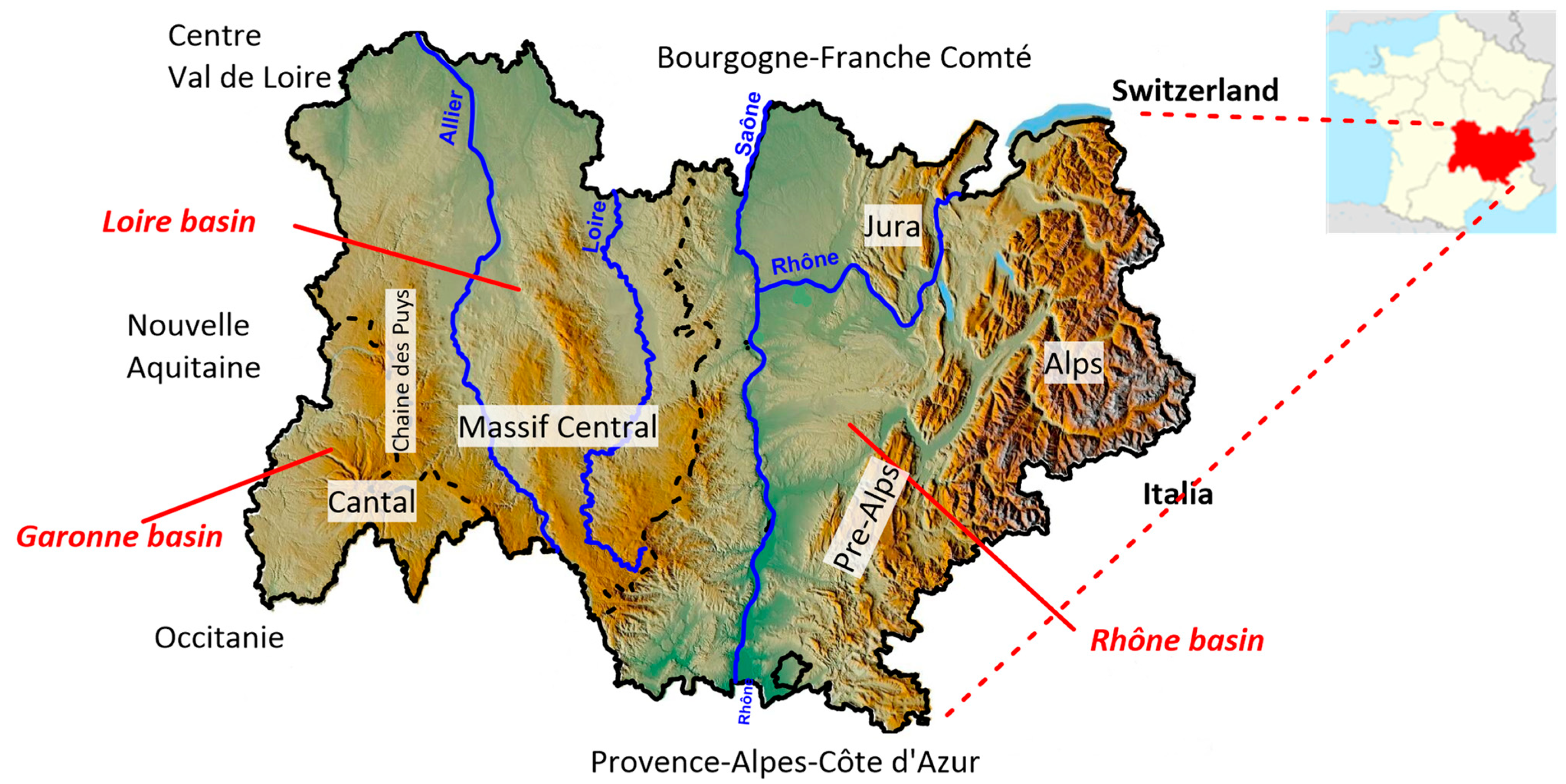
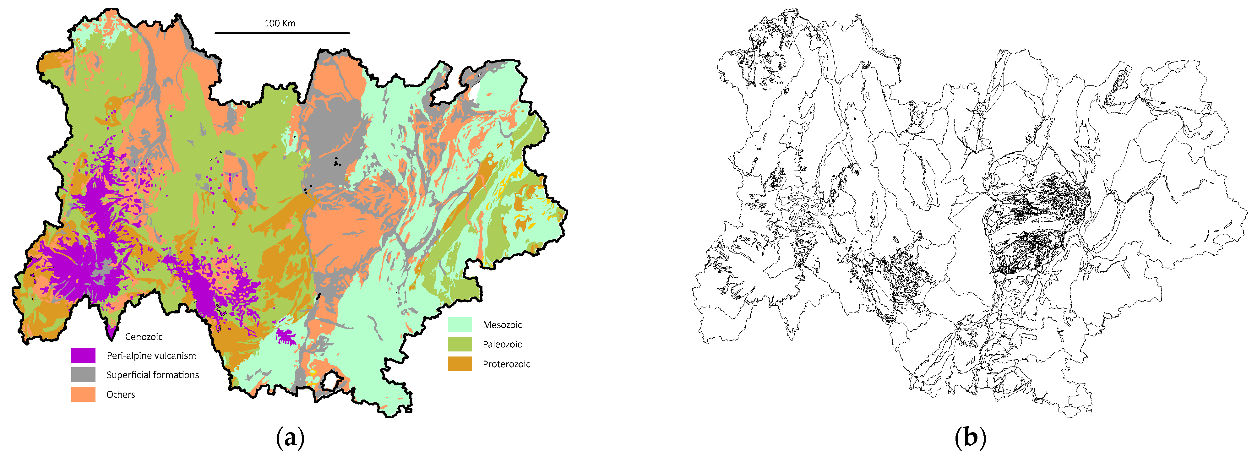
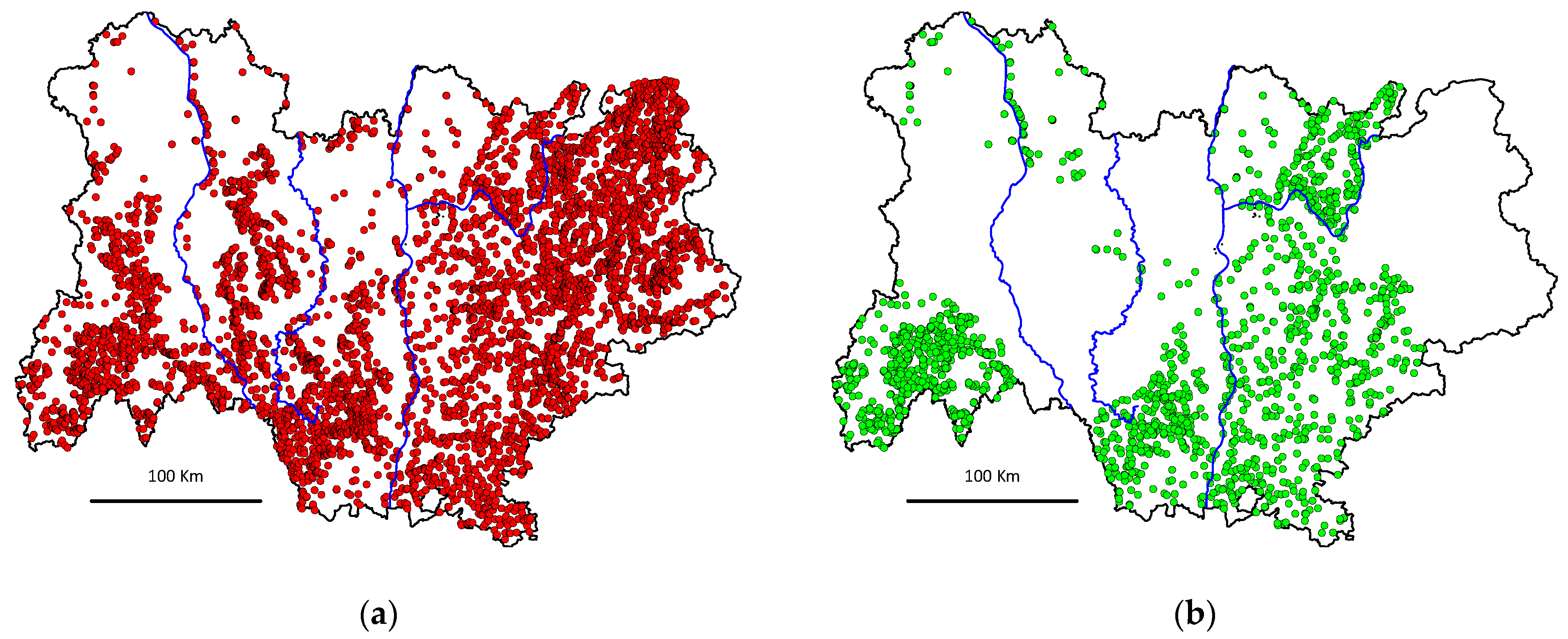
2.1. Auvergne-Rhône-Alpes Region

The Auvergne-Rhône-Alpes region (Figure 1) is located in the southeastern quarter of France, covering an area of 69,711 km² with a population of around 8 million inhabitants [16]. For more details on the geographical aspects of the study area, readers can refer to previous works [14]. The region features complex geology, as it is situated on three major structural units: the Massif Central, the Alps, and the Rhone corridor. To the east, the Alps, with several peaks exceeding 4000 m, are traversed by deep valleys and bordered by limestone Prealps. Further west, the eastern edge of the Massif Central consists of primary rocks in a horst position dominating the grabens of the Rhône and Saône valleys, the Forez plain (Loire Valley), and the Limagne plain (Allier Valley), filled with tertiary and quaternary sediments. The extreme southwest of the region is marked by the volcanic reliefs of Cantal and the Chaîne des Puys (Figure 2a). The region straddles three major watersheds, namely the Rhône basin in its eastern half flowing towards the Mediterranean, the Loire basin to the west, and the Garonne basin in the far southwest, with the latter two flowing towards the Atlantic (Figure 1).

2.2. The French Groundwater Reference System

The European Community’s framework directive of 12 December 2006 (2006/118/EC) encouraged member countries to map not only surface waters but also groundwater bodies (GWB) for monitoring and protection purposes [17,18,19]. This initiative subsequently prompted significant research efforts in EU member states [20,21,22,23,24]. It was referenced according to the major European river basins (Rhône, Rhine, Danube, Loire, Seine, etc.). In France, this inventory was conducted by the French Geological Survey (BRGM), resulting in a French reference system for groundwater bodies (https://services.sandre.eaufrance.fr/geo/sandre, accessed on 7 February 2022). Groundwater bodies are identified by a unique code such as FRXGxxx, where FR refers to France, X designates the major river basin (here, D for the Rhône basin, F for the Garonne basin, and G for the Loire basin), G refers to groundwater, and xxx is a reference number between 001 and 999. In the context of this study, the Auvergne-Rhône-Alpes region encompasses 89 groundwater bodies (Figure 2b), with 60 in the Rhône basin, 21 in the Loire basin, and 8 in the Garonne basin. The number of sample collection points for each basin is provided in

Table 1. Distribution of the number of sampling points (full matrix) and groundwater bodies in the major basins within the Auvergne-Rhône-Alpes region.

	Rhone Basin	Loire Basin	Garonne Basin
Number of sampling points (Full matrix)	1204	481	264
Number of groundwater bodies (GWBs)	60	21	8

and illustrated in Figure 3a,b.

2.3. Sise-Eaux Database

The data used in this study were extracted from the Sise-Eaux database (https://data.eaufrance.fr/concept/sise-eaux, accessed in 15 March 2021). For further details regarding this national database, previous works by our research group [8,9,10,11,12,13,14,15], as well as the basic references [25,26], can be consulted. The extraction conducted for a 30-year period from July 1990 to September 2020 for our study area resulted in a sparse matrix of 114,033 observations (water samples) distributed across 3146 sampling points (Figure 3a), with 21 measured parameters. As calculations in this study cannot be conducted on a sparse matrix, a full matrix was generated by eliminating infrequently analyzed parameters while maximizing the number of observations. The obtained full matrix (Figure 3b) comprises 8078 observations and 13 parameters (major ions, electrical conductivity at 25 °C (E.C.), NO₃, Enterococcus (Ent.), Escherichia coli (E. coli), pH at the sample temperature, Fe). This matrix includes 1949 georeferenced sampling points, averaging 4.15 water samples analyzed per sampling point. In the following, a distinction will be made between values obtained during sample analysis and the variable representing these values; for example, NO₃ is the parameter representing nitrate ion (NO₃⁻) levels.

2.4. Analytical Procedure

The chosen methodology involves 9 steps.

• Consistent with previous studies [10], the data underwent a logarithmic transformation (decimal logarithm) using the formula y = log10(x + DL), where x and DL, respectively, represent the measurement of the physico-chemical or bacteriological parameter X and its detection limit [15]. Only the pH, which already corresponds to the logarithmic transformation of the chemical activity of H₃O⁺, was retained without conditioning. The goal was to align the distributions of each parameter with a normal distribution, but more importantly, to limit the influence of extreme values that could mask certain processes responsible for the variability in water quality within the dataset [11,12].
• Each water sample was then assigned to a groundwater body (GWB) based on its geographical coordinates and depth. At this stage, GWBs with too few analyses (less than 10 water samples collected) were excluded from the analysis.
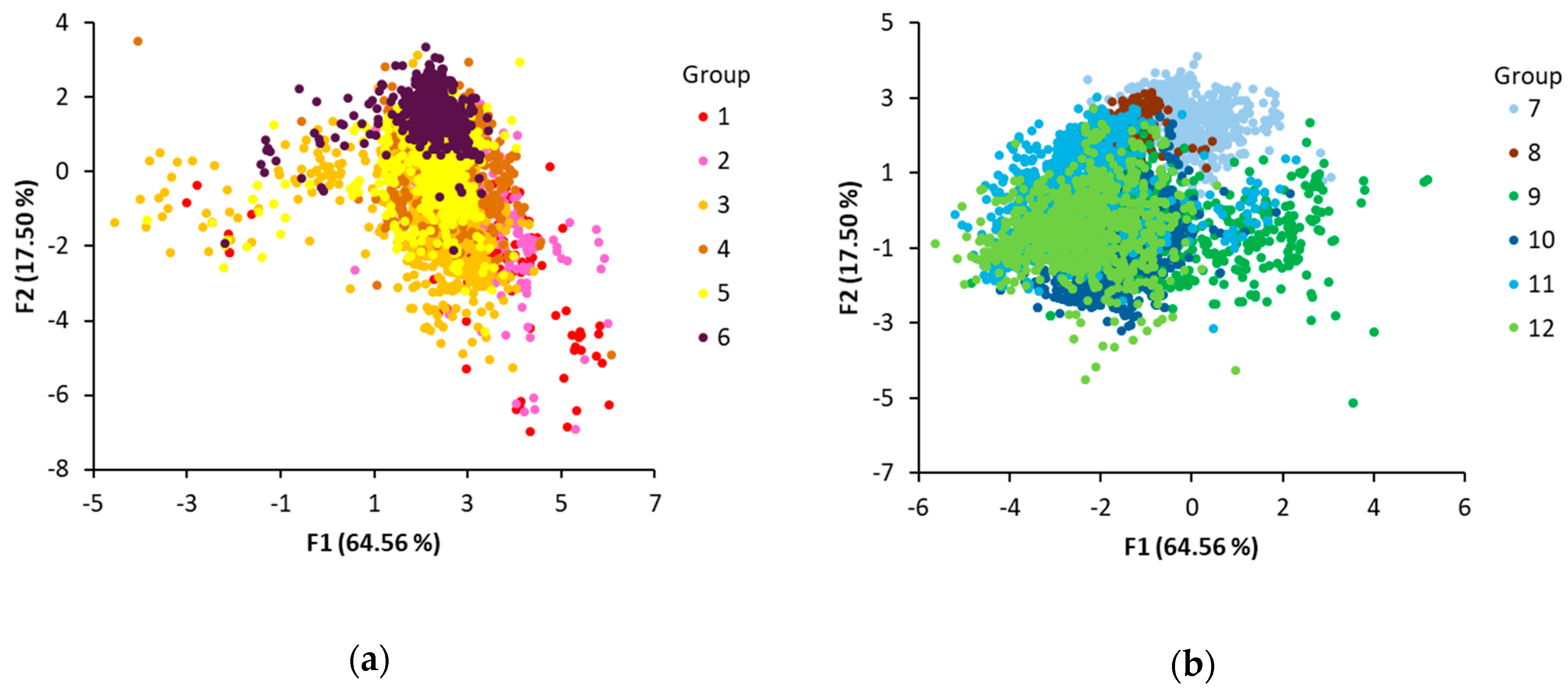
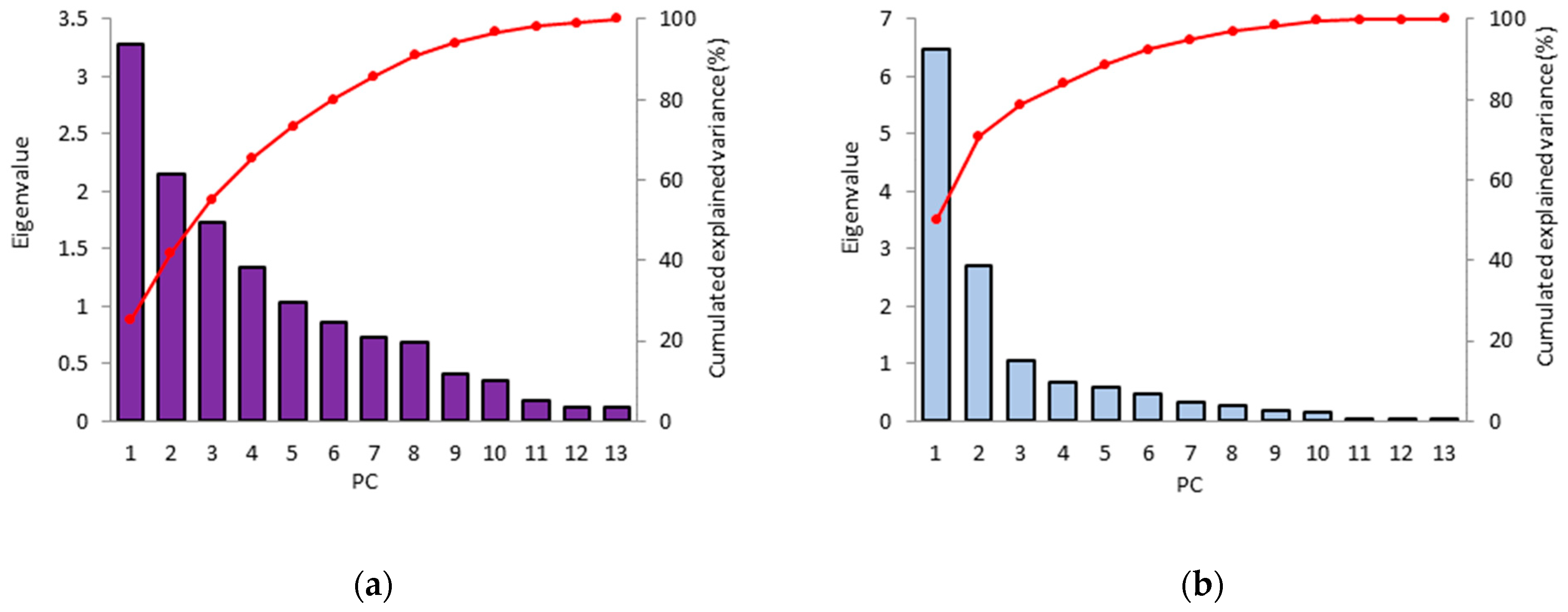
• Principal component analysis (PCA) was subsequently performed on the log-transformed data to reduce the dimensionality of the data space and identify and classify sources of variability within the dataset [27]. PCA is based on the correlation matrix and thus considers standardized variables, allowing the integration of parameters of diverse nature and units (bacteriology, chemistry, etc.). Moreover, it was conducted by diagonalizing the correlation matrix. Under these conditions, the obtained factorial axes are orthogonal to each other in the hyperspace of the data, thus associated with independent processes responsible for water quality variability. The results of this principal component analysis were presented in a previous study [14]. The first six factorial axes, representing 85% of the total variance, were retained for further analysis. The last factorial axes, explaining a small percentage of the variance, were eliminated, considering them to represent background geochemical noise in the dataset [28].
• For each of the selected factorial axes, the average value of the groundwater body (GWB) on the factorial axis was calculated. At this stage, each GWB is characterized by a 6-dimensional vector, with 6 factorial axes being retained.
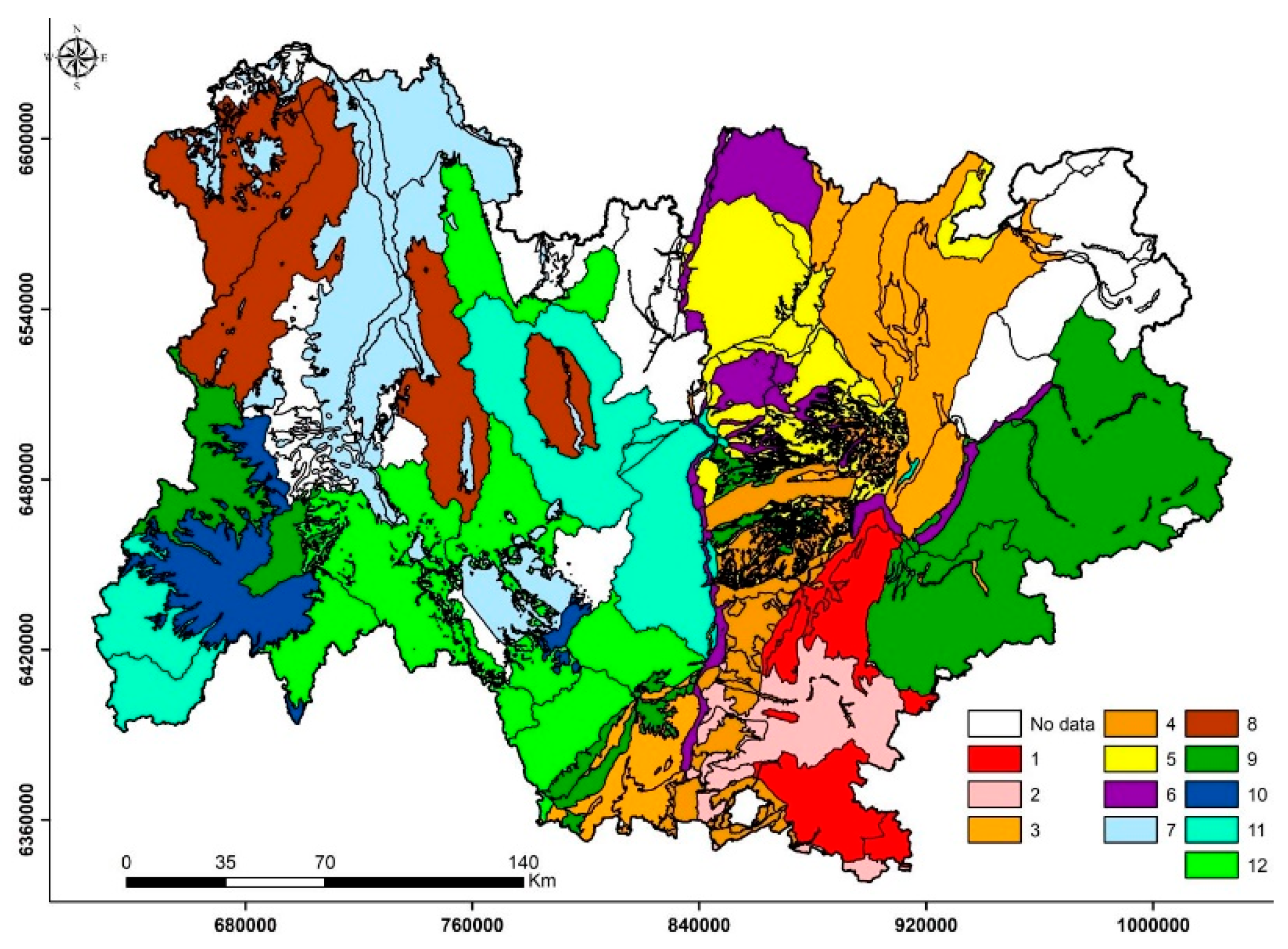
• Unsupervised hierarchical agglomerative clustering (HAC) was performed on all remaining GWBs, assigning equal weight to each of the 6 factorial axes [29,30]. The aim of this clustering was to group GWBs based on a similarity criterion, considering all parameters. The number of groups chosen was guided by the presence of a break in slope in the relationship between the percentage of explained variance and the number of groups, thus maximizing intra-group homogeneity and inter-group heterogeneity. The results were iteratively compiled to produce a dendrogram and presented in map form [31]. For each group, the mean of the parameters was calculated for group comparisons.
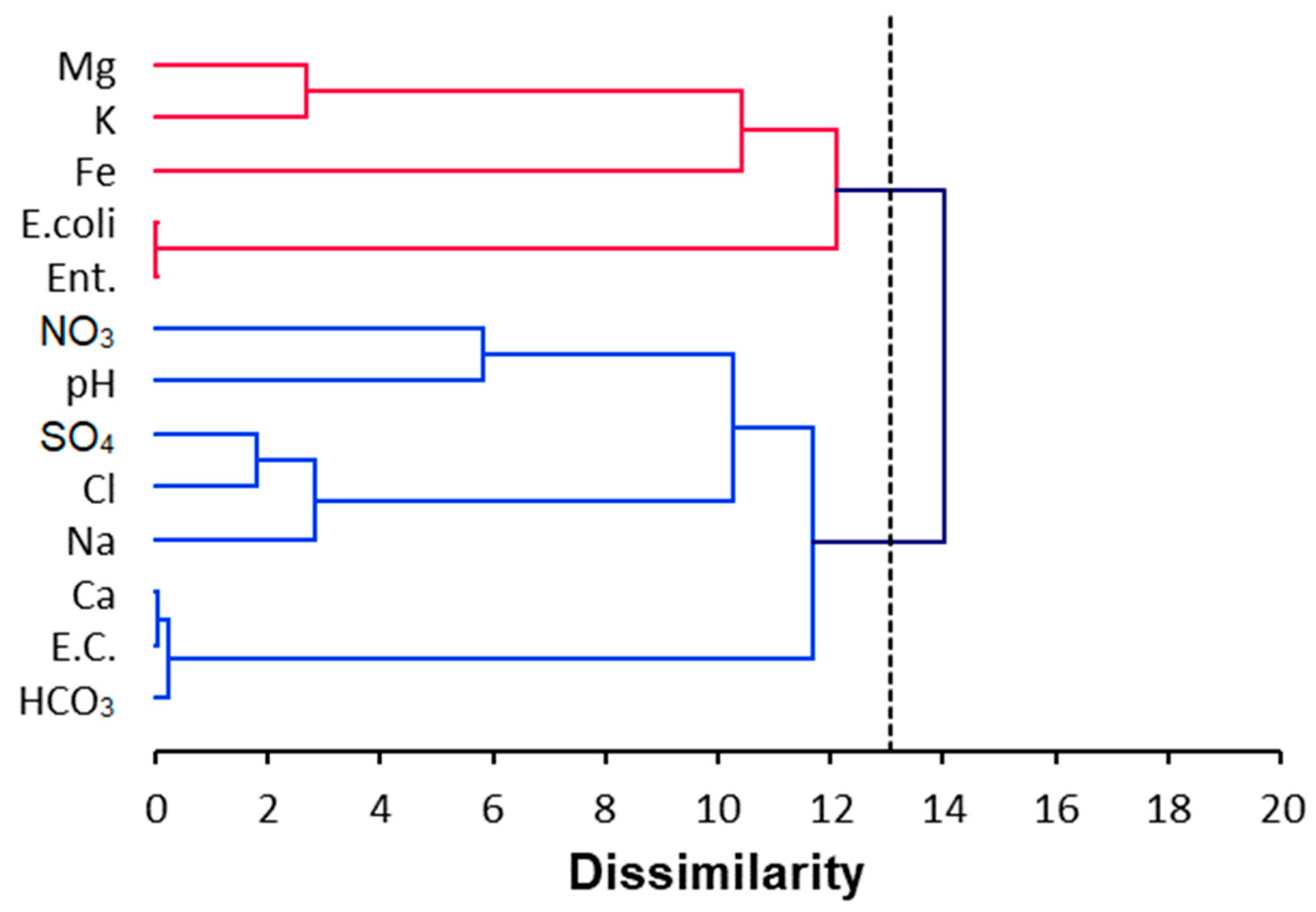
• Ascending hierarchical classification was conducted on all parameters based on their mean values on the first 6 factorial axes of the PCA to detect redundancies in information and behavior among the parameters.
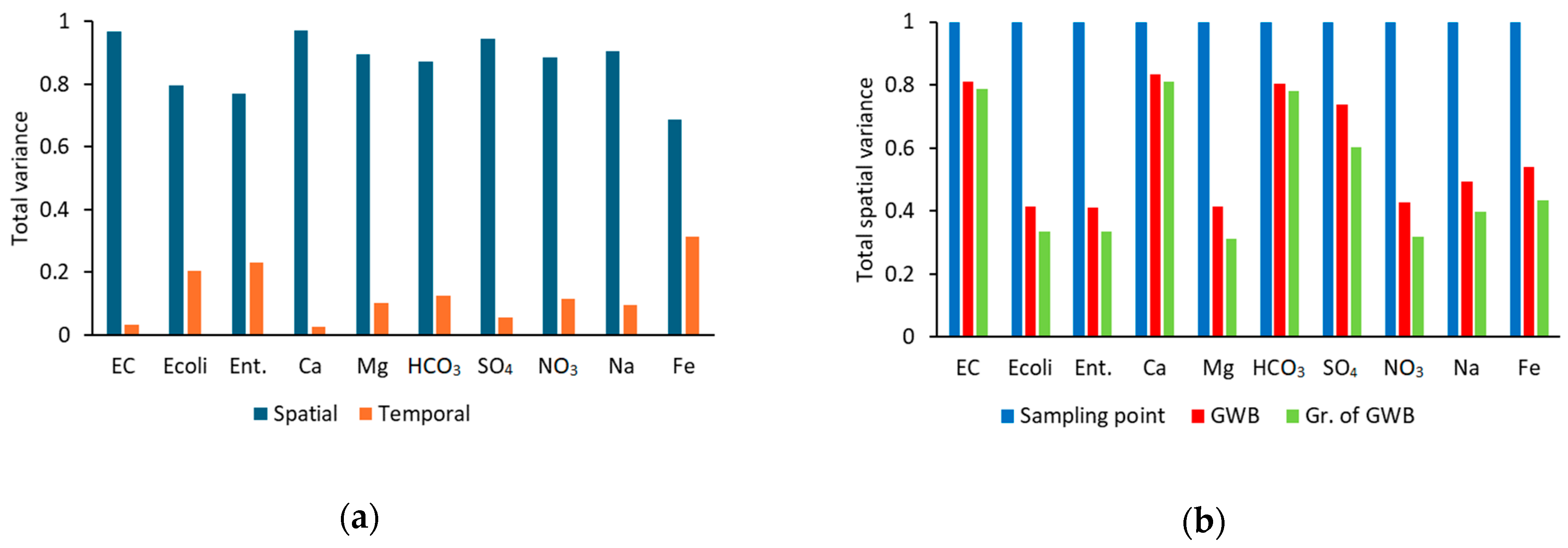
• For each parameter, the information loss induced by aggregating sampling points into GWBs and then into GWB groups was estimated based on the explained variance (R²) using an analysis of variance (ANOVA) [32,33]. Since the analyses were conducted on multiple dates at various sampling points, the total dataset variance includes both temporal variabilities, reflected in different values at the same sampling point, and spatial variability, reflected in different means between sampling points. The R² calculated on the “sampling point” criterion as an explanatory variable corresponds to spatial variability at this scale. The complement to 1 of R², i.e., the fraction of unexplained variance, reflects temporal variance if we neglect a small portion of variance related to analytical imprecision. The same calculation conducted at the GWB and GWB group scales allows quantifying the amount of information contained at these different spatial scales and thus tracking the information loss during grouping [15].
• Linear discriminant analysis (LDA) was conducted to test the possibility of assigning each sample to a sampling point, a groundwater body (GWB), or a group of GWBs based on its chemical and bacteriological composition [34,35]. The GWB groups are established from the mean value of each GWB on the factorial axes. As mentioned earlier, this average includes spatial variability within the GWBs and temporal variability since samples were not collected on the same date. This variability may pose challenges for discriminating each GWB group. LDA serves as an indirect way to assess if differentiation is significant at the sample level. It independently verifies, post hoc, the need to apply the proposed method for determining GWB groups.
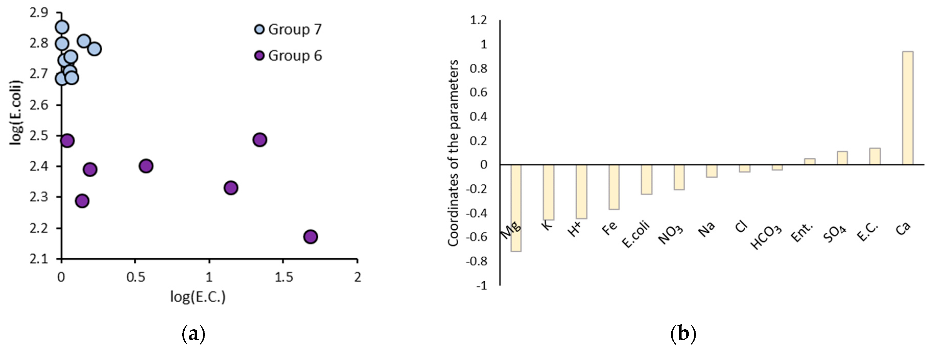
• Finally, a principal component analysis (PCA) and discriminant analysis (LDA) were conducted on two of the obtained groups as an illustrative application to identify the main mechanisms occurring in each group, with the goal of establishing a roadmap for water resource monitoring.

3. Results

3.1. GWB Groups

The 12 homogeneous GWB groups and their degree of dissimilarity are presented in Figure 4. The distribution of these 12 groups across the entire Auvergne-Rhône-Alpes region is presented in Figure 5. Several sectors of the map were notable for lacking data. This absence is not due to a lack of sampling points for quality monitoring but rather to incomplete analyses. Consequently, numerous data points were eliminated during the transition from the sparse matrix (after extraction, 6336 sampling points, 114,033 observations, and 21 parameters, Figure 3a) to the full matrix (1944 sampling points, 8078 observations, and 13 parameters, Figure 3b). The map of GWB groups aligned with the lithology of the area (Figure 2a). Indeed, a discernible distinction existed between the sector with crystalline rocks of the Alps and the Massif Central, the sector with predominantly limestone rocks of the Prealps, the sector with eruptive rocks of Cantal and the Chaîne des Puys, and the more recent sediments of the collapse plains. The distribution of the groups also aligned with the altitude and major structural features of the region. Groups 1 to 7 corresponded to aquifers located in low-altitude areas, such as the valleys of the Rhône, Saône, Loire, and Allier rivers. Groups 8 to 12 were found in the heights of the Massif Central, positioned in horst relative to the collapse plains, in the volcanic sector of the Chaîne des Puys, Cantal, and the Alps. Group 6 encompassed aquifers associated with the main rivers in the Rhône basin and their tributaries, while Group 7 consisted of those from the Loire and Allier rivers. Group 4 related to waters downstream of the Rhône Valley, while Groups 5 and 3 represented upstream areas. Overall, GWB groups belonged to either one or another of the three large basins (Loire, Garonne, or Rhône basin), except for two exceptional groups. The first exception was Group 12, bringing together diluted waters located at the heads of the three major watersheds, as well as high-altitude areas in the Loire basin north of the region. Therefore, this group corresponded to high-altitude GWBs, with the exception of the Alpine sector. The second exception concerned the extensive volcano of Cantal, presenting a conical shape at the boundary between the Loire and Garonne basins. The northeast slope of the volcanic cone, draining towards the Loire basin, was classified in Group 9, which also included several GWBs marked by volcanic terrains but located in the Garonne basin, as well as GWBs in the Alps within the Rhône basin.

The average of different parameters for each group is summarized in

Table 2. Average of parameters for each homogeneous GWB group (data log-transformed in units per 100 mL for bacteriological parameters, in mg L⁻¹ for major ions and nitrates, and in µg L⁻¹ for iron).

Group	Ent.	E. coli	E.C.	pH	K	Na	Ca	Mg	Cl	SO4	HCO3	Fe	NO3
1	0.291	0.309	2.583	7.624	−1.345	−0.029	1.865	0.303	0.355	0.832	2.350	0.538	0.162
2	0.204	0.240	2.700	7.484	−1.125	0.356	1.994	0.556	0.568	1.197	2.476	0.417	0.129
3	0.410	0.501	2.585	7.545	−0.260	0.356	1.837	0.556	0.484	0.828	2.308	1.096	0.430
4	0.075	0.085	2.765	7.419	−0.281	0.752	1.995	0.897	0.911	1.301	2.499	0.509	1.038
5	0.125	0.126	2.693	7.452	−0.058	0.669	1.953	0.629	0.924	0.978	2.362	1.169	1.044
6	0.078	0.078	2.734	7.378	0.174	0.990	1.971	0.764	1.244	1.436	2.393	1.112	1.072
7	1.056	1.255	2.384	7.120	0.538	1.072	1.379	0.770	1.179	1.201	1.949	1.898	0.874
8	1.592	1.853	2.127	7.268	0.412	0.900	1.060	0.488	1.021	0.962	1.637	2.314	0.643
9	0.514	0.580	2.132	7.191	0.067	0.584	1.122	0.609	0.478	0.606	1.796	1.185	0.502
10	0.382	0.395	1.945	6.862	0.116	0.536	0.874	0.520	0.393	0.161	1.613	0.856	0.597
11	0.863	0.962	1.903	6.463	0.138	0.689	0.682	0.276	0.785	0.391	1.256	1.393	0.831
12	0.539	0.593	1.790	6.524	−0.195	0.621	0.636	0.064	0.449	0.472	1.317	1.039	0.388

. The mean values per group were contrasting, with higher variations, particularly as the data are expressed in logarithmic scales in the table. Thus, the development of spatial units of GWB groups did not obscure the regional variations in water quality.

The most mineralized waters were those of Groups 2, 4, 5, and 6. The waters with the lowest mineralization were associated with Groups 10, 11, and 12, situated in the high-altitude regions of the Massif Central, characterized by a lower abundance of carbonates. Table 2 also highlights that mineral content and bacterial contamination play pivotal roles in the variability of water quality and group differentiation. The typology dendrogram of parameters, based on the first six factorial axes of the PCA (Figure 6), underscores the distinct evolution of these two characteristics in the study area. Bacteriological parameters show a stronger association with Fe, Mg, and K, whereas electrical conductivity is more closely linked to other major ions and pH. Figure 7 illustrates the distribution of groups based on the two parameters E.C. and E. coli. Each variable represents one of the two primary parameter groups, providing a comprehensive two-dimensional portrayal of group diversity. The results suggest that highly mineralized waters generally exhibit low bacterial contamination, a trend that increases for groups with intermediate mineral content and decreases for groups with low mineralization.

3.2. Discriminant Analysis

The first two discriminant functions, F1 and F2, are robust and account for 82% of the total discrimination. This initial factorial plane is depicted in Figure 8.

The confusion matrix resulting from the discriminant analysis is presented in

Table 3. Confusion matrix of the discriminant analysis.

from\to	1	2	3	4	5	6	7	8	9	10	11	12	Total	% Correct
1	44	52	40	7	5	1	0	0	0	5	2	0	156	28.21
2	24	100	40	20	11	5	1	0	1	0	0	0	202	49.50
3	10	15	577	32	165	23	7	2	36	7	8	9	891	64.76
4	1	22	69	293	67	51	0	0	5	1	1	0	510	57.45
5	3	8	88	92	757	25	1	0	13	11	0	2	1000	75.70
6	0	3	5	35	110	335	3	0	10	1	1	3	506	66.21
7	0	0	0	0	8	62	356	159	4	0	12	14	615	57.89
8	0	0	0	0	0	0	50	204	0	0	13	1	268	76.12
9	2	6	85	9	23	2	16	13	351	233	86	46	872	40.25
10	0	0	3	0	2	0	8	1	117	851	39	76	1097	77.58
11	0	0	12	0	18	3	25	59	30	64	723	93	1027	70.40
12	1	0	0	0	1	1	9	19	71	94	117	618	931	66.38
Total	85	206	919	488	1167	508	476	457	638	1267	1002	862	8075	64.51

. Across the entire region, 65% of the samples were correctly classified into their respective GWB groups based on chemical and bacteriological composition. The lowest rate of correctly classified samples pertained to Group 1, aquifers located in marly limestone with pyrite, which consequently undergo alteration resulting in higher sulfate concentrations. Group 1 was mainly confused with the geographically adjacent Groups 2 and 3, within sedimentary limestones distributed in the Prealps and Jura. These three groups exhibit mineralized waters with low fecal contamination and appear quite similar in Figure 4 and Figure 7. The highest rates of correct classification were observed for Groups 5, 8, and 10. Group 5 comprises mineralized and less contaminated waters from aquifers associated with the rivers in the Saône and Rhône basins. Group 8 is characterized by a high vulnerability to fecal contamination on the slopes of the Loire and Allier valleys, where cattle farming is predominant. Finally, Group 10 corresponds to waters influenced by volcanic terrains in Cantal and the Chaîne des Puys. The first factorial plane of the discriminant analysis revealed that the differentiation between GWB groups was primarily based on mineral content in a carbonate–calcium context and fecal contamination for waters with a chloride–sodium profile.

3.3. ANOVA, Clustering, and Information Loss

ANOVA was conducted on all analyses measuring the information conveyed by each level of spatial structure concerning the original data, which integrates both spatial and temporal variability. At the sampling point scale, by normalizing the total variance of each parameter to 1, the difference between unity and the variance explained by the sampling points corresponds to the proportion of temporal variability (Figure 9). It encompasses seasonal and multi-year variability, given that the sampling was conducted over 30 years. This temporal variability was more pronounced for bacteriological parameters and iron but less significant for EC, major ions, and nitrates.

The decrease in variance can be understood as the result of information loss during the clustering process. It was observed that this information loss was relatively minimal for major ions and electrical conductivity but more pronounced for bacteriological parameters. Notably, the primary loss of information occurred during the transition from the sampling point scale to the GWB scale. However, the subsequent grouping into homogeneous GWB groups was associated with only marginal information loss despite a significant reduction in the number of spatial units (from 89 GWBs to 12 GWB groups). This pattern was consistent across all parameters (Figure 9b), irrespective of the proportion of temporal variability and the information loss during the initial clustering step (from the sampling point scale to GWBs).

3.4. Detailed Analysis of Groups 6 and 7

Principal component analysis (PCA) conducted on each of these groups indicates that variance is distributed quite differently for the two groups. For Group 6, it is spread across numerous factorial axes, with the first five principal components (PCs) having eigenvalues greater than one (Figure 10a). The sources of variability in water characteristics are thus numerous and of relatively comparable intensity, justifying a detailed study. Conversely, the majority of the variance is captured by the first two factorial axes for Group 7, indicating a lower number of mechanisms impacting water characteristics (Figure 10b). Discriminant analysis conducted on the entire set of 1121 water samples (506 for Group 6 and 615 for Group 7) shows a very high discrimination rate of 97%. The waters from these two groups differentiate in terms of mineral content and calcium concentration, specifically in the Ca/Mg ratio (Figure 11b). Group 7 is affected by very severe and recurrent fecal contaminations across all groundwater bodies (GWB), whereas these contaminations are much less frequent and less severe for sampling points in Group 6, as indicated by Figure 11a representing the average values for each GWB along the mineral content and fecal contamination axes.

4. Discussion

4.1. Criteria for Group Discrimination

Existing groundwater databases focus on one or several properties or characteristics of groundwater, such as water levels, hydrochemistry, water resources, and basin recharge rates. Therefore, applying big data technology to groundwater associated with other earth sciences proves challenging, requiring original data and relatively comprehensive groundwater properties [36]. It is indeed recognized that many environmental/hydrological management questions cannot be adequately addressed by single-discipline studies [37]. The intersection between the Sise-Eaux database and the French reference system for groundwater bodies is a fruitful illustration, combining high-quality data with an independent geographic feature of GWB delimitation, enabling the adequate addressing of numerous environmental management questions.

In our previous investigation, we underscored the intricacy of information within the same database, necessitating the retention of at least six factorial axes to encompass 85% of the variance—equivalent to about 85% of the data’s informational content [14]. This intricacy arises from the diverse natural settings found in this expansive region, encompassing variations in altitudes, lithologies, groundwater resources, climate, and human activities. Moreover, it reflects the multitude of mechanisms contributing to water quality. The grouping of groundwater bodies (GWBs) into homogeneous sets should therefore help better discriminate these mechanisms [12]. The GWB groups derived from the Auvergne-Rhône-Alpes region primarily consist of geographically proximate GWBs, forming cohesive geographical clusters based on lithological attributes. These include regions with crystalline rocks in the Alps and the Massif Central, eruptive rocks in Cantal and the vicinity of the Chaîne des Puys, sedimentary rocks in the Prealps and Jura, and recent sediments in the valleys of collapse (such as the Rhône Valley, Loire, and Allier valleys). Correspondingly, the GWB groups align with variations in altitude and major structural features. The least mineralized waters are located in high-altitude areas, consistent with a shorter water-rock contact time and lower temperature at higher altitudes, which slows down rock weathering. The increase in mineral content from high to low areas in the region is accompanied by an increase in carbonate alkalinity and pH, in line with the rock weathering process, especially in more limestone lithologies. The obtained grouping of GWBs, therefore, makes sense. In addition to water mineral content, fecal contamination is a major criterion for distinguishing GWB groups. The highest contaminations are observed in Groups 6, 7, and 11, specifically in the Massif Central regions where cattle farming is prevalent, both in the Loire and Garonne basins. In the Rhône basin, the inverse relationship between fecal contamination and mineral content can be attributed to the flocculating power of cations on clay colloids, which are the primary carriers of microorganisms during water runoff at the surface of soils [38,39].

4.2. A Minimal Loss of Information

The results of the ANOVA confirm the effectiveness of the method for discriminating homogeneous groups of GWBs. The grouping of sampling points into GWBs, independently delineated for our study by geologists and hydrogeologists from the French Geological Survey, inevitably leads to an information loss associated with a significant reduction in the number of spatial units (from 1944 sampling points to 89 GWBs). However, grouping the information to achieve a manageable number of units for groundwater resource monitoring is accompanied by minimal information loss. Overall, the transition from 1944 sampling points to only 12 GWB groups results in a spatial information loss of about 20% for major ions and approximately 50% for other water quality parameters. These quantitative results demonstrate the effectiveness of the proposed method, and in this regard, the set objective has been achieved.

4.3. Method Applicability

A similar study conducted in the Occitanie region [12], of comparable size to the Auvergne-Rhône-Alpes region, highlighted the need to divide the region into two contrasting major basins from a climatic perspective (Mediterranean Rhône and Adour-Garonne) to minimize information loss during the grouping of GWBs. This result was in line with the requirements for the GWB inventory under the European Framework Directive, which imposes compartmentalization by major catchment area [19]. In Auvergne-Rhône-Alpes, the presence of three major basins does not pose an obstacle to the application of the grouping method. The fact that groups generally distribute within one or the other of the major basins justifies, in a way, the European Water Framework Directive recommending an inventory of GWBs based on the division of major European basins. The number of 89 GWBs delineated by the French Geological Survey across the entire region is excessive for targeted and effective monitoring of water quality by the Regional Health Agency. In contrast, the 12 GWB groups correspond to homogeneous units in terms of physico-chemical and bacteriological characteristics, as well as in terms of the mechanisms responsible for acquiring these characteristics. This facilitates the development of a roadmap for quality monitoring.

4.4. Examples of Roadmaps for Monitoring Groups 6 and 7

The study reveals that riverbank aquifers are not all grouped into a single category. A distinction is made between those in the Rhône basin and those in the Loire and Allier basins. Groups 6 and 7 only converge with a dissimilarity of about 230 in the hierarchical clustering (Figure 4), considering all parameters. The riverbank aquifers of the Loire and Allier, originating in the crystalline and volcanic environments of the Massif Central, form Group 7 of GWBs. It differs significantly from Group 6, which includes aquifers accompanying major rivers in the Rhône basin, such as the Rhône, Saône, and their main tributaries. The Saône-Rhône axis, downstream of their confluence, creates a north–south separation between the Massif Central with crystalline and volcanic lithology to the west and the alpine zone with limestone rocks from the Jurassic, marly limestones from the Cretaceous, sometimes highly mineralized Triassic rocks, and some granite sectors from the central Alps (Figure 2a). This results in a considerable lithological heterogeneity in the drainage basins fed by these watercourses. These alluvial valleys serve as transportation routes in mountainous areas and areas of population concentration in major cities. Being in a low position, the valleys collect water from the surrounding slopes. Consequently, although their coverage on the map is relatively limited (Figure 5), these riverbank aquifers constitute the most important groundwater resources in the region and are therefore of strategic importance for the water supply to major cities such as Lyon, as well as all medium-sized cities in the Rhône Valley and the Loire and Allier valleys. These aquifers are generally well-protected against bacterial contamination and undergo intensive monitoring by public authorities. As a result, Groups 6 and 7 have relatively comprehensive data, with 10 GWBs and 506 water samples for Group 6 and 7 GWBs and 615 water samples for Group 7.

Overall, contaminations are evident during identifiable dilution periods characterized by lower mineral content. These episodes typically occur during rainy periods when surface waters, laden with bacteria from surface runoff, contaminate sampling points [38,39,40]. The transport of germs in water requires solid phases, such as suspended matter (T.S.S.), which disperse and detach more easily from the soil when the water’s content of flocculant divalent ions (such as calcium) is low. The abundance of fecal-origin bacteria (E. coli and Enterococci) is negatively correlated with water mineral content (E.C.), calcium content, and carbonate alkalinity. Conversely, it is positively correlated with iron content, likely associated with colloidal iron. In summary, sampling points in Group 7 pose a significantly higher risk of fecal contamination compared to those in Group 6. This difference is linked to mineral content, particularly calcium levels. For both groups, the risk is higher during wet periods, such as intense rain events like late summer storms. Thus, in practical terms, heightened vigilance will be required during rainy periods in the Group 7 area, while surveillance for Group 6 can be less stringent. This interpretation of fecal contamination relies on a main assumption, which is that contamination is observed during intense rainfall events that promote runoff and germ transport. In the future, it will be necessary to find a treatment that will confirm, or at least refine this hypothesis. A study based on the separation of spatial and temporal variance within these extensive databases could be attempted.

5. Conclusions

This study, which aimed to establish a limited number of spatial units for the optimized monitoring of water resources, is based on the intersection of two databases: the French reference for groundwater bodies and the monitoring of groundwater quality by regional health agencies. Despite the large size of the region, it is possible to discriminate 12 homogeneous groundwater body (GWB) groups based on chemical and bacteriological composition, as well as on the mechanisms responsible for the diversity of these characteristics. The fact that the region spans three major watersheds (Rhône, Loire, and Garonne) does not hinder the application of the grouping method. The grouping of 89 GWBs into 12 groups is facilitated by well-structured topographical and geological contrasts, with minimal information loss, validating the method. The prediction of membership for a given sample in a GWB group is mediocre, emphasizing the importance of working with the averages of each GWB when applying this grouping method. The homogeneity of the groups facilitates the identification of ongoing mechanisms responsible for the diversity within each group, allowing the establishment of a roadmap for resource monitoring. The two groups examined in this study, corresponding to riverbank aquifers, show that despite a similar topographical position, the intensity of bacterial contamination differs significantly, highlighting the role of flocculent cation levels in bacterial transport. Future work will focus on a detailed analysis and the development of a roadmap for the protection and monitoring of each of these 12 groups, but also on separating the study of spatial and temporal variance within these extensive databases to refine the various pathways of fecal contamination.

References

1. van der Gun, J. Chapter 24-Groundwater Resources Sustainability; Mukherjee, A., Scanlon, B.R., Aureli, A., Langan, S., Guo, H., McKenzie, A.A., Eds.; Elsevier: Amsterdam, The Netherlands, 2021; pp. 331–345. ISBN 978-0-12-818172-0. [Google Scholar]
2. Yuan, H.; Yang, S.; Wang, B. Hydrochemistry characteristics of groundwater with the influence of spatial variability and water flow in Hetao Irrigation District, China. Environ. Sci. Pollut. Res. 2022, 29, 71150–71164. [Google Scholar] [CrossRef]
3. Gao, Y.; Chen, J.; Qian, H.; Wang, H.; Ren, W.; Qu, W. Hydrogeochemical characteristics and processes of groundwater in an over 2260 year irrigation district: A comparison between irrigated and nonirrigated areas. J. Hydrol. 2022, 606, 127437. [Google Scholar] [CrossRef]
4. Bhunia, G.S.; Shit, P.K.; Brahma, S. Chapter 19-Groundwater Conservation and Management: Recent Trends and Future Prospects; Shit, P., Bhunia, G., Adhikary, P., Eds.; Elsevier: Amsterdam, The Netherlands, 2023; pp. 371–385. ISBN 978-0-323-99963-2. [Google Scholar]
5. Koundouri, P. Current Issues in the Economics of Groundwater Resource Management. J. Econ. Surv. 2004, 18, 703–740. [Google Scholar] [CrossRef]
6. Kemper, K.E. Groundwater—From development to management. Hydrogeol. J. 2004, 12, 3–5. [Google Scholar] [CrossRef]
7. Beaudeau, P.; Pascal, M.; Mouly, D.; Galey, C.; Thomas, O. Health risks associated with drinking water in a context of climate change in France: A review of surveillance requirements. J. Water Clim. Chang. 2011, 2, 230–246. [Google Scholar] [CrossRef]
8. Tiouiouine, A.; Jabrane, M.; Kacimi, I.; Morarech, M.; Bouramtane, T.; Bahaj, T.; Yameogo, S.; Rezende-Filho, A.; Dassonville, F.; Moulin, M.; et al. Determining the relevant scale to analyze the quality of regional groundwater resources while combining groundwater bodies, physicochemical and biological databases in southeastern france. Water 2020, 12, 3476. [Google Scholar] [CrossRef]
9. Tiouiouine, A.; Yameogo, S.; Valles, V.; Barbiero, L.; Dassonville, F.; Moulin, M.; Bouramtane, T.; Bahaj, T.; Morarech, M.; Kacimi, I. Dimension reduction and analysis of a 10-year physicochemical and biological water database applied to water resources intended for human consumption in the provence-alpes-cote d’azur region, France. Water 2020, 12, 525. [Google Scholar] [CrossRef]
10. Jabrane, M.; Touiouine, A.; Bouabdli, A.; Chakiri, S.; Mohsine, I.; Valles, V.; Barbiero, L. Data Conditioning Modes for the Study of Groundwater Resource Quality Using a Large Physico-Chemical and Bacteriological Database, Occitanie Region, France. Water 2023, 15, 84. [Google Scholar] [CrossRef]
11. Mohsine, I.; Kacimi, I.; Abraham, S.; Valles, V.; Barbiero, L.; Dassonville, F.; Bahaj, T.; Kassou, N.; Touiouine, A.; Jabrane, M.; et al. Exploring Multiscale Variability in Groundwater Quality: A Comparative Analysis of Spatial and Temporal Patterns via Clustering. Water 2023, 15, 1603. [Google Scholar] [CrossRef]
12. Jabrane, M.; Touiouine, A.; Valles, V.; Bouabdli, A.; Chakiri, S.; Mohsine, I.; El Jarjini, Y.; Morarech, M.; Duran, Y.; Barbiero, L. Search for a Relevant Scale to Optimize the Quality Monitoring of Groundwater Bodies in the Occitanie Region (France). Hydrology 2023, 10, 89. [Google Scholar] [CrossRef]
13. Mohsine, I.; Kacimi, I.; Valles, V.; Leblanc, M.; El Mahrad, B.; Dassonville, F.; Kassou, N.; Bouramtane, T.; Abraham, S.; Touiouine, A.; et al. Differentiation of multi-parametric groups of groundwater bodies through Discriminant Analysis and Machine Learning. Hydrology 2023, 10, 230. [Google Scholar] [CrossRef]
14. Ayach, M.; Lazar, H.; Bousouis, A.; Touiouine, A.; Kacimi, I.; Valles, V.; Barbiero, L. Multi-Parameter Analysis of Groundwater Resources Quality in the Auvergne-Rhône-Alpes Region (France) Using a Large Database. Resources 2023, 12, 143. [Google Scholar]
15. Lazar, H.; Ayach, M.; Barry, A.; Mohsine, I.; Touiouine, A.; Huneau, F.; Mori, C.; Garel, E.; Kacimi, I.; Valles, V.; et al. Groundwater bodies in Corsica: A critical approach to GWBs subdivision based on multivariate water quality criteria. Hydrology 2023, 10, 213. [Google Scholar] [CrossRef]
16. DRAAF-Occitanie Cartothèque (Regularly Updated). Available online: https://draaf.occitanie.agriculture.gouv.fr/cartotheque-r101.html (accessed on 7 January 2023).
17. Chave, P. The EU Water Framework Directive-An Introduction; IWA Publishing: London, UK, 2007; ISBN 9781780402239. [Google Scholar]
18. Kallis, G.; Butler, D. The EU water framework directive: Measures and implications. Water Policy 2001, 3, 125–142. [Google Scholar] [CrossRef]
19. European Commission Directive 2006/118/EC of the European Parliament and of the Council of 12 December 2006 on the protection of groundwater against pollution and deterioration. Off. J. Eur. Union 2006, 372, 19–31.
20. Wendland, F.; Blum, A.; Coetsiers, M.; Gorova, R.; Griffioen, J.; Grima, J.; Hinsby, K.; Kunkel, R.; Marandi, A.; Melo, T.; et al. European aquifer typology: A practical framework for an overview of major groundwater composition at European scale. Environ. Geol. 2008, 55, 77–85. [Google Scholar] [CrossRef]
21. Duscher, K. Compilation of a Groundwater Body GIS Reference Layer. In Proceedings of the Presentation at the WISE GIS Workshop, Copenhagen, Denmark, 16–17 November 2010. [Google Scholar]
22. Irish Working Group on Groundwater. Approach to Delineation of Groundwater Bodies, Guidance Document No.2; IWGG: Dublin, Ireland, 2005. [Google Scholar]
23. Moral, F.; Cruz-Sanjulián, J.J.; Olías, M. Geochemical evolution of groundwater in the carbonate aquifers of Sierra de Segura (Betic Cordillera, southern Spain). J. Hydrol. 2008, 360, 281–296. [Google Scholar] [CrossRef]
24. Psomas, A.; Bariamis, G.; Roy, S.; Rouillard, J.; Stein, U. Comparative Study on Quantitative and Chemical Status of Groundwater Bodies: Study of the Impacts of Pressures on Groundwater in Europe; Service Contract, 315/B2020/EEA.58185; EEA: Brussels, Belgium, 2021. [Google Scholar]
25. Chery, L.; Laurent, A.; Vincent, B.; Tracol, R. Echanges SISE-Eaux/ADES: Identification des Protocoles Compatibles Avec les Scénarios D’échange SANDRE; InfoTerre: Vincennes/Orléans, France, 2011. [Google Scholar]
26. Gran-Aymeric, L. Un portail national sur la qualite des eaux destinees a la consommation humaine. Tech. Sci. Méthodes 2010, 12, 45–48. [Google Scholar] [CrossRef]
27. Helena, B.; Pardo, R.; Vega, M.; Barrado, E.; Fernandez, J.M.; Fernandez, L. Temporal evolution of groundwater composition in an alluvial aquifer (Pisuerga River, Spain) by principal component analysis. Water Res. 2000, 34, 807–816. [Google Scholar] [CrossRef]
28. Rezende-Filho, A.T.; Valles, V.; Furian, S.; Oliveira, C.M.S.C.; Ouardi, J.; Barbiero, L. Impacts of lithological and anthropogenic factors affecting water chemistry in the upper Paraguay River Basin. J. Environ. Qual. 2015, 44, 1832–1842. [Google Scholar] [CrossRef]
29. Day, W.H.E.; Edelsbrunner, H. Efficient algorithms for agglomerative hierarchical clustering methods. J. Classif. 1984, 1, 7–24. [Google Scholar] [CrossRef]
30. Bouguettaya, A.; Yu, Q.; Liu, X.; Zhou, X.; Song, A. Efficient agglomerative hierarchical clustering. Expert Syst. Appl. 2015, 42, 2785–2797. [Google Scholar] [CrossRef]
31. Brugeron, A. Cartographie et Systèmes D’Information Géographique Pour La Gestion Des Ressources En Eau Souterraine. 2012. Available online: https://brgm.hal.science/hal-01182473/document (accessed on 17 March 2020).
32. Miles, J. R-Squared, Adjusted R-Squared. In Encyclopedia of Statistics in Behavioral Science; John Wiley & Sons, Ltd.: Hoboken, NJ, USA, 2005; ISBN 9780470013199. [Google Scholar]
33. Woldt, W.; Bogardi, I. Ground water monitoring network design using multiple criteria decision making and geostatistics. JAWRA J. Am. Water Resour. Assoc. 1992, 28, 45–62. [Google Scholar] [CrossRef]
34. Huberty, C.J. Discriminant Analysis. Rev. Educ. Res. 1975, 45, 543–598. [Google Scholar] [CrossRef]
35. Amiri, V.; Nakagawa, K. Using a linear discriminant analysis (LDA)-based nomenclature system and self-organizing maps (SOM) for spatiotemporal assessment of groundwater quality in a coastal aquifer. J. Hydrol. 2021, 603, 127082. [Google Scholar] [CrossRef]
36. Qiu, W.; Ma, T.; Wang, Y.; Cheng, J.; Su, C.; Li, J. Review on status of groundwater database and application prospect in deep-time digital earth plan. Geosci. Front. 2022, 13, 101383. [Google Scholar] [CrossRef]
37. Fitch, P.; Brodaric, B.; Stenson, M.; Booth, N. Integrated Groundwater Data Management BT-Integrated Groundwater Management: Concepts, Approaches and Challenges; Jakeman, A.J., Barreteau, O., Hunt, R.J., Rinaudo, J.-D., Ross, A., Eds.; Springer International Publishing: Cham, Switzerland, 2016; pp. 667–692. ISBN 978-3-319-23576-9. [Google Scholar]
38. Boithias, L.; Choisy, M.; Souliyaseng, N.; Jourdren, M.; Quet, F.; Buisson, Y.; Thammahacksa, C.; Silvera, N.; Latsachack, K.; Sengtaheuanghoung, O.; et al. Hydrological Regime and Water Shortage as Drivers of the Seasonal Incidence of Diarrheal Diseases in a Tropical Montane Environment. PLoS Negl. Trop. Dis. 2016, 10, e0005195. [Google Scholar] [CrossRef]
39. Pachepsky, Y.A.; Shelton, D.R. Escherichia Coli and Fecal Coliforms in Freshwater and Estuarine Sediments. Crit. Rev. Environ. Sci. Technol. 2011, 41, 1067–1110. [Google Scholar] [CrossRef]
40. Abbas, A.; Baek, S.; Silvera, N.; Soulileuth, B.; Pachepsky, Y.; Ribolzi, O.; Boithias, L.; Cho, K.H. In-stream Escherichia coli modeling using high-temporal-resolution data with deep learning and process-based models. Hydrol. Earth Syst. Sci. 2021, 25, 6185–6202. [Google Scholar] [CrossRef]
Figure 1. Physical setting of the study site, Auvergne-Rhône-Alpes region, France.
Water 16 00869 g001
Figure 2. (a) Simplified lithological map of the study area, and (b) delineation of the 89 groundwater bodies (GWB) identified by the French Geological Survey.
Water 16 00869 g002
Figure 3. Distribution of sampling points in the study area for (a) the sparse matrix and (b) the full matrix used for discriminating GWB groups.
Water 16 00869 g003
Figure 4. Dendrogram resulting from hierarchical agglomerative clustering leading to the discrimination of 12 homogeneous groundwater body (GWB) groups. The small inset dendrogram refers to the entire population.
Water 16 00869 g004
Figure 5. Distribution of homogeneous GWB groups across the Auvergne-Rhône-Alpes region. The GWBs left in blank are those for which the quantity of data was insufficient within the full matrix.
Water 16 00869 g005
Figure 6. Dendrogram of parameter typology based on their average values across the first 6 principal components (8078 samples).
Water 16 00869 g006
Figure 7. Comparison of groups obtained by hierarchical clustering based on mineral content and bacterial contamination criteria (averages calculated for each group). Note an inverse relationship between bacterial contamination and electrical conductivity for the most mineralized waters (dotted line).
Water 16 00869 g007
Figure 8. Representation of the first factorial plane of the discriminant analysis for (a) Groups 1 to 6 and (b) 7 to 12.
Water 16 00869 g008
Figure 9. (a) Temporal and spatial variance at the sampling point scale for each parameter; (b) decrease in the spatial variance from the scale of the sampling point (normalized at 1) to that of the GWB, and then to the GWB groups.
Water 16 00869 g009
Figure 10. Inertia of the factorial axes for (a) Group 6 and (b) Group 7.
Water 16 00869 g010
Figure 11. Comparison of Groups 6 and 7; (a) average values of groundwater bodies (GWB) along the axes of mineral content and fecal contamination and (b) canonical coefficients of discriminant function F1, which accounts for 97% of the discrimination between the two groups.
Water 16 00869 g011