Assessing Objective Functions in Streamflow Prediction Model Training Based on the Naïve Method

Abstract

Reliable streamflow forecasting is a determining factor for water resource planning and flood control. To better understand the strengths and weaknesses of newly proposed methods in streamflow forecasting and facilitate comparisons of different research results, we test a simple, universal, and efficient benchmark method, namely, the naïve method, for short-term streamflow prediction. Using the naïve method, we assess the streamflow forecasting performance of the long short-term memory models trained with different objective functions, including mean squared error (MSE), root mean squared error (RMSE), Nash–Sutcliffe efficiency (NSE), Kling–Gupta efficiency (KGE), and mean absolute error (MAE). The experiments over 273 watersheds show that the naïve method attains good forecasting performance (NSE > 0.5) in 88%, 65%, and 52% of watersheds at lead times of 1 day, 2 days, and 3 days, respectively. Through benchmarking by the naïve method, we find that the LSTM models trained with squared-error-based objective functions, i.e., MSE, RMSE, NSE, and KGE, perform poorly in low flow forecasting. This is because they are more influenced by training samples with high flows than by those with low flows during the model training process. For comprehensive short-term streamflow modeling without special demand orientation, we recommend the application of MAE instead of a squared-error-based metric as the objective function. In addition, it is also feasible to perform logarithmic transformation on the streamflow data. This work underscores the critical importance of appropriately selecting the objective functions for model training/calibration, shedding light on how to effectively evaluate the performance of streamflow forecast models.

1. Introduction

Water serves as a critical elemental resource essential for both the sustenance and progress of humanity. However, with the impact of global climate change and human activities, the availability of water resources is steadily diminishing [1]. The efficient and rational utilization of water resources has, thus, emerged as a global concern. Streamflow, being the primary accessible water resource for human beings, necessitates the implementation of appropriate engineering and non-engineering measures, such as reservoir operation and water resource dispatching, as effective strategies for optimizing their utilization. Reliable short-term streamflow forecasting stands as a crucial assurance for the smooth implementation of these methods [2]. Conversely, flooding remains one of the major natural meteorological disasters worldwide, characterized by sudden onset, extensive reach, and severity. Currently, streamflow forecasting also plays a pivotal role in responding to and mitigating such floods. The advanced and reliable prediction of basin streamflow serves as essential guidance for flood prevention and mitigation efforts [3].

In the early days, studies on hydrological models generally focused on isolated hydrological processes, yielding seminal theoretical concepts and formulas. Notable among these are the unit hydrograph concept proposed by Sherman [4], Horton’s runoff production theory [5], and the Penman Monteith equation for evaporation calculation [6]. With a better understanding of the comprehensive hydrological processes (e.g., infiltration, soil water movement, runoff generation, and evapotranspiration), the concept of a “watershed hydrological model” was developed to describe the various aspects of watershed hydrological processes as an integrated system [7]. Hydrological researchers have proposed various aggregate hydrological models with abstract generalized equations describing basin hydrological processes, such as the Xinanjiang model [8], the tank model [9], the SCS model [10], and the API model [11]. The concept of the distributed hydrological model was first introduced by Freeze and Harlan in 1969. Compared with the aggregate hydrological models, these models consider the spatial heterogeneity of meteorological condition, model parameters, and interactions between individual hydrological processes over the entire basin. These advancements promote an understanding of model mechanisms and improve model performance. The most prominent distributed hydrological models include HEC-HMS [12], MIKE11 [13], SWAT [14], and WRF-Hydro [15].

In recent years, there has been a notable surge in the utilization of data-driven approaches in hydrological studies, owing to the exponential growth of hydrometeorological data and advancements in algorithms [16,17,18,19]. Among these approaches, deep learning methods have gained considerable traction, demonstrating considerable promise. Numerous studies have underscored their efficacy in streamflow simulations/predictions, often outperforming traditional process-based models [20,21,22]. Frame et al. [23] identified a critical limitation inherent in process-based models like the National Water Model, highlighting their tendency to lose crucial information during the propagation from atmospheric forcing inputs to outputs. This loss of information ultimately leads to suboptimal performance compared to deep learning models. Similarly, Nearing et al. [24] illustrated how deep learning methods hold the potential to mitigate uncertainties arising from issues such as downscaling atmospheric forcing data to watershed scales and errors in hydrological model structure and parameter estimation during streamflow prediction model development.

In a deep learning model, the determination of numerous parameters is crucial during model training. The choice of the objective function holds paramount importance as it significantly influences the calibrated values of model parameters and thereby impacts the model outputs [25]. In previous research, squared-error-based metrics, such as mean squared error (MSE) and root mean squared error (RMSE), have been widely employed as objective functions for streamflow predictions [26]. For example, Granata et al. [27] utilized squared error as the objective function when training the MLP model to forecast daily streamflow across four watersheds. Feng et al. [21] employed RMSE to minimize the disparity between predicted streamflow and USGS observations. The Nash–Sutcliffe efficiency (NSE) is a normalized version of MSE [28], representing the ratio of the error of the forecast model to the error obtained by considering the observational mean as the forecast. Despite certain limitations associated with NSE [29], its usage has gained momentum in recent studies focusing on streamflow prediction [30,31].

In hydrological modeling studies, establishing baseline models is a common practice. Typically, these models are constructed using methods that have undergone extensive scrutiny and have exhibited commendable modeling performance. Comparing these models against baseline models offers valuable insights into the advancements or limitations of newly proposed or applied methods. For instance, Ghobadi and Kang [32] applied LSTM-BNN, BNN, and LSTM with Monte Carlo dropout as benchmarks to evaluate the proposed Bayesian long short-term memory model, demonstrating the superiority of the probabilistic forecasting approach over deterministic models for multi-step-ahead daily streamflow forecasting. Similarly, Lin et al. [33] showcased the advantages of machine learning algorithms over statistical methods for hourly streamflow prediction by benchmarking against multiple linear regression, autoregressive moving average, and autoregressive integrated moving average models. Furthermore, some studies have employed process-based models as benchmarks for evaluating deep learning models (e.g., Frame et al. [22], Kratzert et al. [34], and Kratzert et al. [35]). However, it is essential to note that benchmarking the entire spectrum of existing hydrological modeling approaches is impractical. Researchers typically select benchmark models based on their expertise or personal preference, leading to a situation where modeling approaches are not consistently and effectively compared and evaluated across research, especially in diverse regional case studies. This challenge has, to some extent, impeded the progress of hydrological modeling research [24].

In this study, we examined a straightforward and effective benchmark approach for short-term streamflow prediction known as the naïve method, which relies on the inherent characteristics of streamflow series. We conducted a comprehensive evaluation of this method across 273 watersheds in the continental United States. Additionally, we employed the long short-term memory network (LSTM) to establish streamflow forecasting models. Through benchmarking against the naïve method, we evaluate model performances using various metrics as objective functions, including MSE, RMSE, NSE, Kling–Gupta efficiency (KGE), and mean absolute error (MAE). The remainder of this paper is structured as follows: Section 2 outlines the methods and data utilized in this study. The experimental results and discussion are presented in Section 3 and Section 4, respectively, followed by a conclusion in Section 5.

2. Materials and Methods

2.1. Naïve Method

In the context of this study, the naïve method involves making predictions for daily streamflow by simply taking the streamflow value of the current day and using it as the forecast for subsequent days [36]. This method capitalizes on the high temporal autocorrelation commonly observed in short-term streamflow series, making it a reasonable approach for short-term forecasting tasks. Specifically, the naïve method assumes that the future streamflow values will be similar to the current value due to the persistence of short-term patterns in the data.

The naïve method is well suited to serve as a baseline for benchmarking other forecasting models due to its simplicity, universality, and effectiveness in short-term streamflow forecasting. Firstly, it is applicable to virtually all current studies, as it solely relies on the streamflow observation sequence, a fundamental requirement for evaluating and potentially training models in these studies. Secondly, its operational simplicity is noteworthy, as it merely involves shifting the observation sequence. Lastly, predictions generated by the naïve method are generally acceptable or even excellent, often exhibiting hydrological signatures that closely resemble the observed data (as demonstrated in Section 3.1).

2.2. Long Short-Term Memory Model

In this study, we apply long short-term memory (LSTM) to establish the streamflow forecasting models. LSTM is a well-established neural network model that can be used to efficiently process sequential data [37]. It controls the input, processing, forgetting, and output processes of the data through the internal gating structures. In recent years, there have been an increasing number of studies that applied LSTM for streamflow forecasting and produced positive outcomes, e.g., Feng et al. [21], Granata et al. [27], Zhong et al. [38], and Vatanchi et al. [39]. Numerous studies have highlighted LSTM’s superior performance across diverse applications [22,40,41]. For instance, Yuan et al. demonstrated LSTM’s higher accuracy in predicting monthly runoff compared to other models [42]. Wang et al. found LSTM to outperform backpropagation neural network (BP-NN) and online sequential extreme learning machine (OS-ELM) models in water quality forecasting [43]. Additionally, Bowes et al. observed LSTM’s improved predictive capabilities over original RNNs in forecasting the groundwater table response to storm events in a coastal environment [44]. We do not provide a detailed account about the structure of LSTM in this paper, because that is not the focus of this study. More detailed descriptions of LSTM can been seen in pertinent literature such as Hochreiter and Schmidhuber [45] and Kratzert et al. [35].

The LSTM models established in this study consist of two standard LSTM layers, each of which is unidirectional and contains 48 neurons. Following the last LSTM layer, a single dense layer with 96 neurons is employed to project the results to the final output. The dense layer utilizes the ReLU activation function [46] to rectify negative values, as negative streamflow values lack meaningful interpretation. Adam [47] is used to optimize the LSTM models, which amalgamates two widely-used algorithms, Adagrad (effective for handling sparse gradients) and RMSProp (suitable for non-stationary data).

2.3. Objective Functions for LSTM Training

The objective function plays an important role during the LSTM training process, and the choice of the objective function can substantially affect the quality of the trained model [25]. At present, the widely used objective functions are squared-error-based metrics (such as MSE and RMSE), which have a squared error term in their mathematical expressions. In this study, we respectively test the streamflow forecasting performance of the LSTM models when trained with four different squared-error-based objective functions, including MSE, RMSE, NSE, and KGE.

MSE and RMSE serve as fundamental metrics by providing an assessment of the average squared deviation between predicted and observed streamflow values. Their sensitivity to outliers and ability to capture overall variability make them valuable tools for quantifying prediction accuracy. NSE offers a normalized measure of model performance relative to a benchmark, typically the mean observed streamflow. Its range from negative infinity to unity allows for intuitive comparisons across different models and datasets, facilitating comprehensive assessments of predictive skill. KGE combines multiple facets of model performance, including correlation, bias, and variability, into a single metric. By simultaneously considering these aspects, KGE offers a balanced evaluation of both the accuracy and reliability of streamflow predictions, providing valuable insights for model refinement and decision-making processes. The mathematical expressions of these four objective functions are as in Equations (1)–(4), respectively:

$$\mathrm{M}\mathrm{S}\mathrm{E}=\frac{1}{N}{\sum }_{i=1}^N{\left(x_{o,i}-x_{s,i}\right)}^2$$

(1)

$$\mathrm{R}\mathrm{M}\mathrm{S}\mathrm{E}=\sqrt{\frac{{\sum }_{i=1}^N{\left(x_{o,i}-x_{s,i}\right)}^2}{N}}$$

(2)

$$\mathrm{N}\mathrm{S}\mathrm{E}=1-\frac{{\sum }_{i=1}^N{\left(x_{o,i}-x_{s,i}\right)}^2}{{\sum }_{i=1}^N{\left(x_{o,i}-{\mu }_o\right)}^2}$$

(3)

$$\mathrm{K}\mathrm{G}\mathrm{E}=1-\sqrt{s_r\times {(r-1)}^2+s_{\alpha }\times {(\alpha -1)}^2+s_{\beta }\times {(\beta -1)}^2}$$

(4)

$$r=\frac{\frac{1}{N}{\sum }_{i=1}^N\left(x_{o,i}-{\mu }_s\right)-(x_{m,i}-{\mu }_s)}{\sqrt{{\sum }_{i=1}^N{(x_{o,i}-{\mu }_o)}^2}\times \sqrt{{\sum }_{i=1}^N{(x_{s,i}-{\mu }_s)}^2}}$$

(5)

$$\alpha =\frac{{\sigma }_s}{{\sigma }_o}$$

(6)

$$\beta =\frac{{\mu }_s}{{\mu }_o}$$

(7)

where $x_{o,i}$ and $x_{s,i}$ are the observation and model prediction, respectively. $N$ represents the total number of samples. ${\mu }_o$ and ${\mu }_s$ represent the mean of the observation and the prediction, respectively. ${\sigma }_o$ and ${\sigma }_s$ represent the standard deviations of the observation and the prediction, respectively. $s_r$, $s_{\alpha }$, and $s_{\beta }$ in Equation (4) are the scaling factors that can be used to re-scale the criteria space. In this study, we experiment with two combinations of settings. In the first setting, $s_r$, $s_{\alpha }$, and $s_{\beta }$ are set to be 1, 1, and 1, respectively, while in the second one, they are set to be 1, 2, and 1, respectively. For convenience, these two settings are denoted as KGE111 and KGE121, respectively.

For comparison, we also test the prediction performance of the LSTM when MAE is used as the objective function. The mathematical expression of MAE does not have a squared error term, as shown in Equation (8). MAE provides a straightforward measure of the average absolute deviation between predicted and observed streamflow values. Its simplicity and robustness to outliers make it particularly useful for focusing on the magnitude of errors, offering clear insights into model accuracy.

$$\mathrm{M}\mathrm{A}\mathrm{E}=\frac{1}{N}{\sum }_{i=1}^N\left|x_{s,i}-x_{o,i}\right|$$

(8)

In addition, considering the fact that the streamflow data typically belong to a long-tail distribution, we apply a log transform to the streamflow series before training the LSTM models with MSE as the objective function, as shown in Equation (9).

$$x_{o,i}^t={log}_{10}\left(\sqrt{x_{o,i}}+0.1\right)$$

(9)

For convenience, in this paper, the LSTM models trained with the objective functions of MSE, RMSE, NSE, KGE111, KGE121, and MAE are represented by LSTM_MSE, LSTM_RMSE, LSTM_NSE, LSTM_KGE111, LSTM_KGE121, and LSTM_MAE, respectively. The LSTM models trained based on the log-transformed streamflow data with MSE as the objective function are represented by LSTM_MSE(log).

2.4. Evaluation Metrics

In this study, we use five evaluation metrics to assess the models’ prediction performance, including MAPE, NSE, KGE, α, and β. MAPE is calculated by Equation (10), and the expressions of NSE, KGE, α, and β are shown as Equations (3), (4), (6), and (7), respectively.

$$\mathrm{M}\mathrm{A}\mathrm{P}\mathrm{E}=\frac{1}{N}{\sum }_{i=1}^N\frac{\left|x_{s,i}-x_{o,i}\right|}{x_{o,i}}$$

(10)

2.5. Data

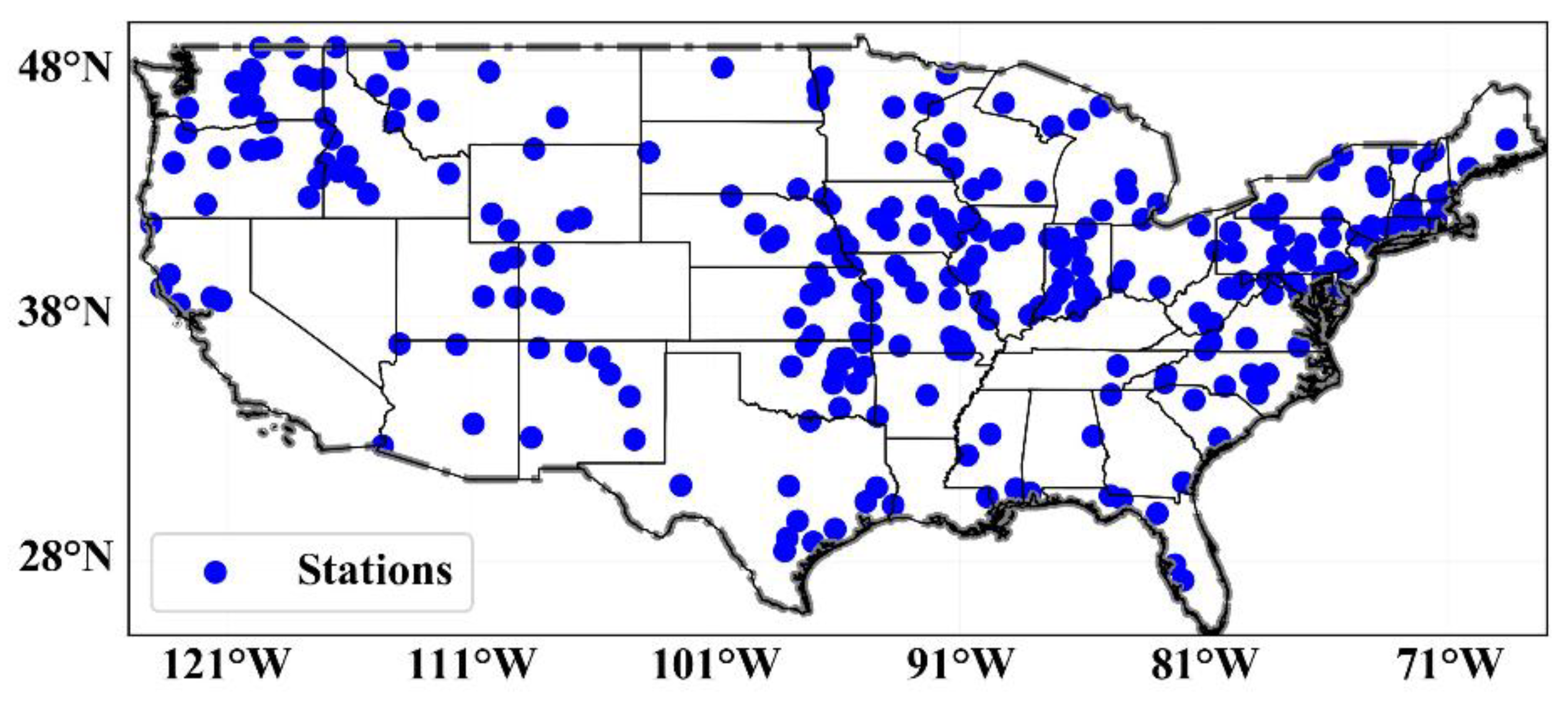
The hydrological data used in this study include streamflow, precipitation, temperature, and evaporation. Among them, the streamflow data were obtained from the Global Runoff Data Centre (GRDC). Here, 273 stations with complete daily streamflow data series from 1982 to 2018 in the USA were chosen, and their locations are displayed in Figure 1. The corresponding precipitation, temperature, and evaporation data were obtained from the North America Land Data Assimilation System version 2 (NLDAS-2).

In this study, we establish LSTM models separately for each watershed. The inputs of the LSTM models are the daily streamflow, daily precipitation, daily temperature, and daily evaporation within the previous 10 days, resulting in 40 inputs in total per sample. The output of the models is the predicted streamflow with lead times ranging from 1 to 3 days. Additionally, the data from 1982 to 2013 are used for the model training, while the remaining data from 2014 to 2018 are preserved as the testing set.

3. Results

3.1. Forecasting Performance of the Naïve Method

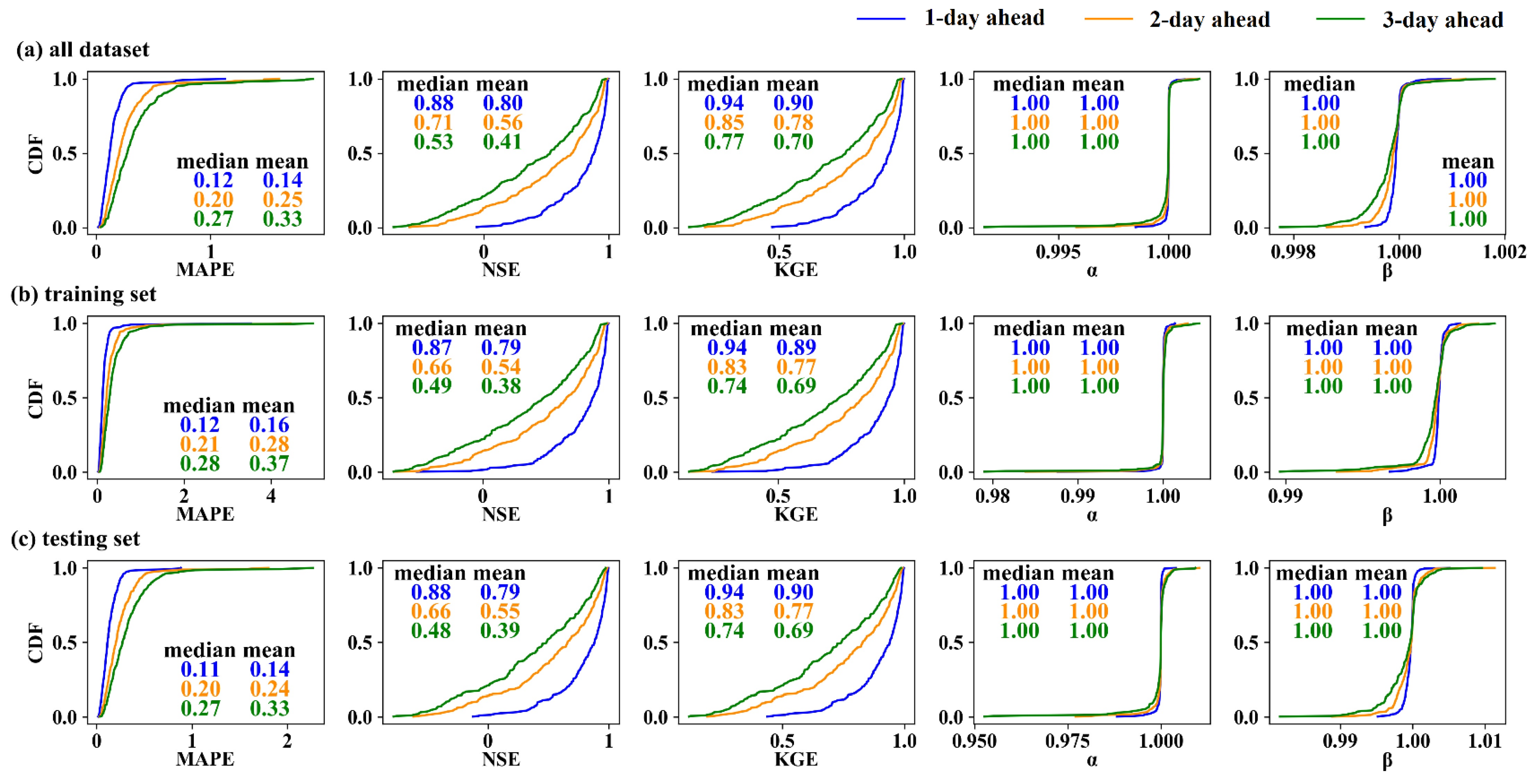
Figure 2 shows the forecast performance of the naïve method at different lead times. Since the naïve method does not require training data to calibrate the model, as conventional modeling methods do, we assess the method using the entire dataset (Figure 2a). It is observed that the naïve method achieves remarkable performance for 1-day-ahead streamflow forecasting. The medians of MAPE, NSE, and KGE in the whole dataset are 0.12, 0.88, and 0.94, respectively, while the means are 0.14, 0.80, and 0.90, respectively. Generally, predictions with NSE greater than 0.5 are considered good. Our results indicate that 88% of the watersheds achieve good predictions using the naïve method. α and β are two metrics measuring the difference in the standard deviations and mean of streamflow series between observations and predictions, respectively. Since the prediction from the naïve method can be regarded as the shift in the observational time series, it exhibits almost perfect α and β, with values in the CDF plot very close to one. As the lead time increases, the forecasting performance deteriorates, yet remains within an acceptable range. For 3-day-ahead forecasting, the medians of MAPE, NSE, and KGE in the entire dataset are 0.27, 0.53, and 0.77, respectively. The proportions of watersheds with an NSE greater than 0.5 for 2-day-ahead and 3-day-ahead forecasting are 65% and 52%, respectively. To facilitate later comparison with LSTM, we also illustrate the evaluations for the training (Figure 2b) and testing (Figure 2c) sets, respectively. While slight differences exist in the assessment between the training and testing sets, the overall evaluation results remain favorable. Additionally, their performances are similar to those in the entire dataset.

3.2. Benchmarking the LSTM Models by the Naïve Method

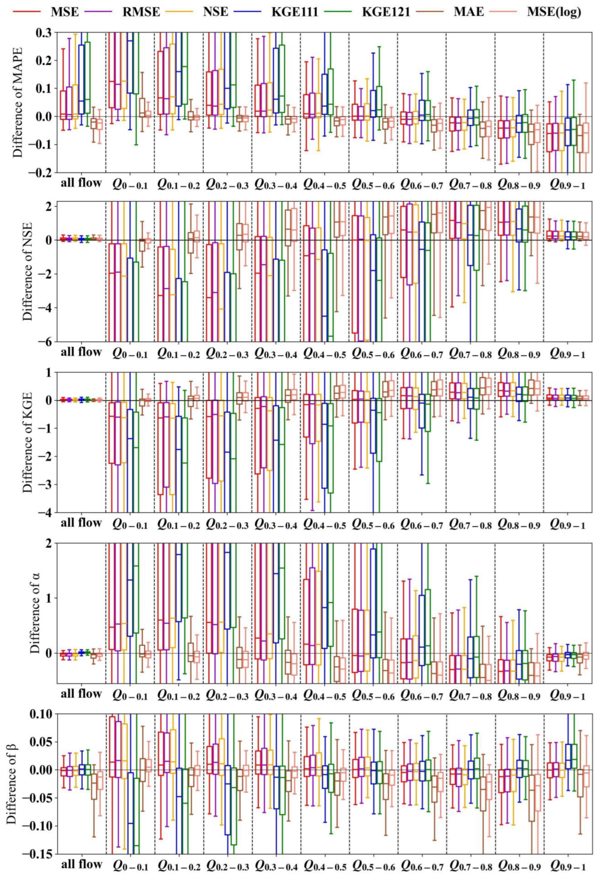
To investigate the forecasting performance of LSTM models trained with different objective functions, we evaluate these models against the forecasting results from the naïve model in terms of various statistical metrics in the testing set, as shown in Figure 3. When assessed across all streamflow levels, the LSTM models trained with squared-error-based objective functions, including MSE, RMSE, NSE, KGE111, and KGE121, outperform the naïve method in terms of NSE and KGE, but exhibit poorer performance in terms of MAPE. According to the metric α results, LSTM_MSE, LSTM_RMSE, and LSTM_NSE tend to underestimate the variance of the streamflow, whereas LSTM_KGE111 and LSTM_KGE121 tend to overestimate it. In addition, the metric β results indicate that the models calibrated with the squared-error-based objective functions are able to reasonably capture the mean of the observational streamflow.

However, when evaluating the forecasting performance separately across different streamflow levels, the results can vary significantly. Generally, models trained with squared-error-based objective functions excel over the naïve method in high flow forecasting, although the degree of superiority diminishes with decreasing streamflow levels. All five models, including LSTM_MSE, LSTM_RMSE, LSTM_NSE, LSTM_KGE111, and LSTM_KGE121, are notably inferior to the naïve method in low flow forecasting. Furthermore, models trained with KGE111 and KGE121 exhibit poorer forecasting performance compared to models trained with MSE, RMSE, and NSE. Applying MAE as the objective function or performing a log transformation on the original streamflow series can enhance the prediction effectiveness for low flows to some extent. The forecasting performance of LSTM_MAE and LSTM_MSE(log) for very low flows, i.e., Q_0–0.1 (where subscript represents the percentile range), is comparable to that of the naïve method. However, LSTM_MAE and LSTM_MSE(log) perform slightly poorer than LSTM_MSE in terms of high flow forecasting and are less effective at capturing the mean and variance of the observations.

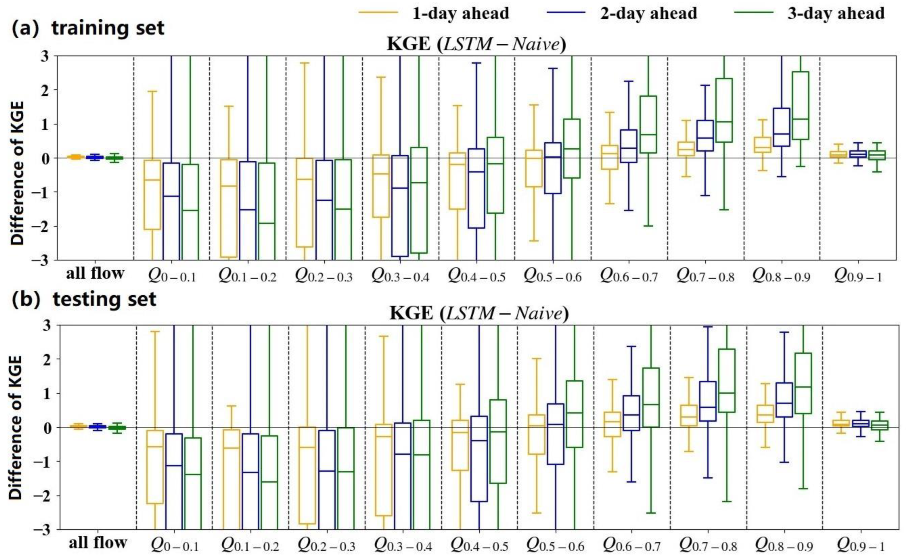
To explore the effect of lead time on model performance, we take LSTM_MSE as an example to show the difference in prediction performance between the LSTM model and the naïve method at three different lead times, as shown in Figure 4. It is found that LSTM_MSE at the lead times of 2 days and 3 days performs similarly to that at the 1-day lead time. LSTM_MSE outperforms the naïve method for high flow prediction, but significantly underperforms for low flow prediction. However, the variation in the LSTM_MSE prediction across all streamflow levels increases with the increase in the lead time. For high flow forecasting, LSTM_MSE is superior to the naïve method at the 3-day lead time compared to the 1-day lead time, whereas for low flow forecasting, the reverse is true.

4. Discussion

4.1. Characteristics of the Naïve Method

The short-term streamflow series inherently exhibits a high autocorrelation in time, which is the key factor ensuring the prediction effectiveness of the naïve method. Feng et al. [21] demonstrated that incorporating historical streamflow as model input can significantly enhance daily-scale streamflow prediction. Similarly, Lin et al. [33] utilized the Shapley Additive Explanations (SHAP) method to analyze the hourly scale streamflow forecasting model and discovered that the contribution of lagged streamflow to the forecast results outweighs that of lagged precipitation by a significant margin.

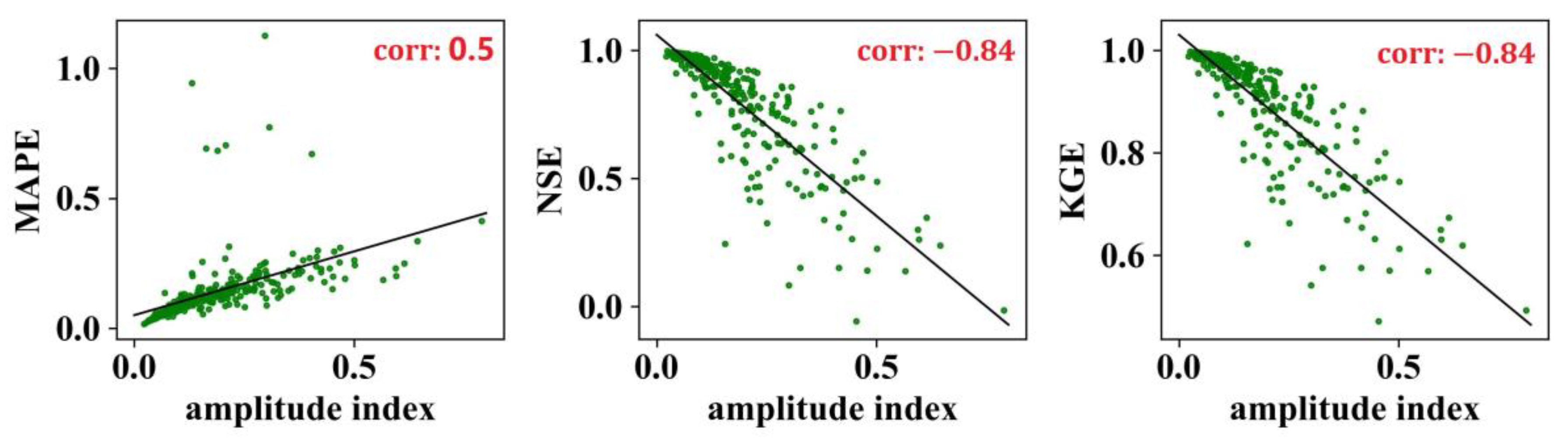
We calculate the amplitude index (AI) of the streamflow series for each watershed according to the formula $\mathrm{A}\mathrm{I}=\frac{1}{{\mu }_o}·\frac{1}{N-1}·{\sum }_{i=2}^N\left|x_{o,i}-x_{o,i-1}\right|$, and then analyze the relationship between the AI and the prediction performance of the naïve method. According to Figure 5, the prediction effect of the naïve method shows a significant negative correlation with AI. The lower the AI, the better the evaluations for the corresponding predictions made by the naïve method. The correlation coefficients between AI and the metric MAPE, NSE, and KGE are 0.5, −0.84, and −0.84, respectively, and all of them pass the significance test at the 5% significance level. These findings indicate that watersheds with lower AI values may represent more stable and predictable hydrological systems, where the naïve method can produce accurate predictions and is suitable to be a baseline. Conversely, watersheds with higher AI values, indicating greater variability in streamflow amplitude, may pose challenges for the naïve method, leading to less accurate predictions.

As illustrated in the preceding results, the autocorrelation present in the streamflow series enables the naïve method to produce predictions with remarkable performance. Moreover, since the predictions from the naïve method essentially entail shifting the observed streamflow series by one day or several days, they possess additional commendable attributes. As demonstrated in Section 3.1, predictions generated by the naïve method exhibit nearly identical mean and standard deviations, as observed in the data. Additionally, several hydrological signatures in the predictions from the naïve method closely resemble those observed in the data, including baseflow index and recession shapes.

4.2. Selection of Objective Function

4.2.1. Importance of Objective Function

The choice of objective function in training serves as a crucial guide, directing the model towards minimizing specific errors or maximizing performance metrics. When the chosen objective function aligns well with the task requirements, the model tends to exhibit superior generalization capabilities. For instance, in sequence prediction tasks, employing an objective function that penalizes sequence-level errors is more suitable than focusing solely on individual predictions. Moreover, different objective functions can lead the model to prioritize different aspects of the data or to learn different representations. For example, some objective functions may encourage the model to focus more on capturing high flow patterns, while others may prioritize low flow patterns. The behavior induced by the objective function during training can affect how well the model generalizes to unseen data. If the objective function encourages the model to capture relevant patterns in the data that are also present in unseen examples, the model is likely to exhibit robust generalization.

4.2.2. Flaw of the Squared Error-Based Objective Function

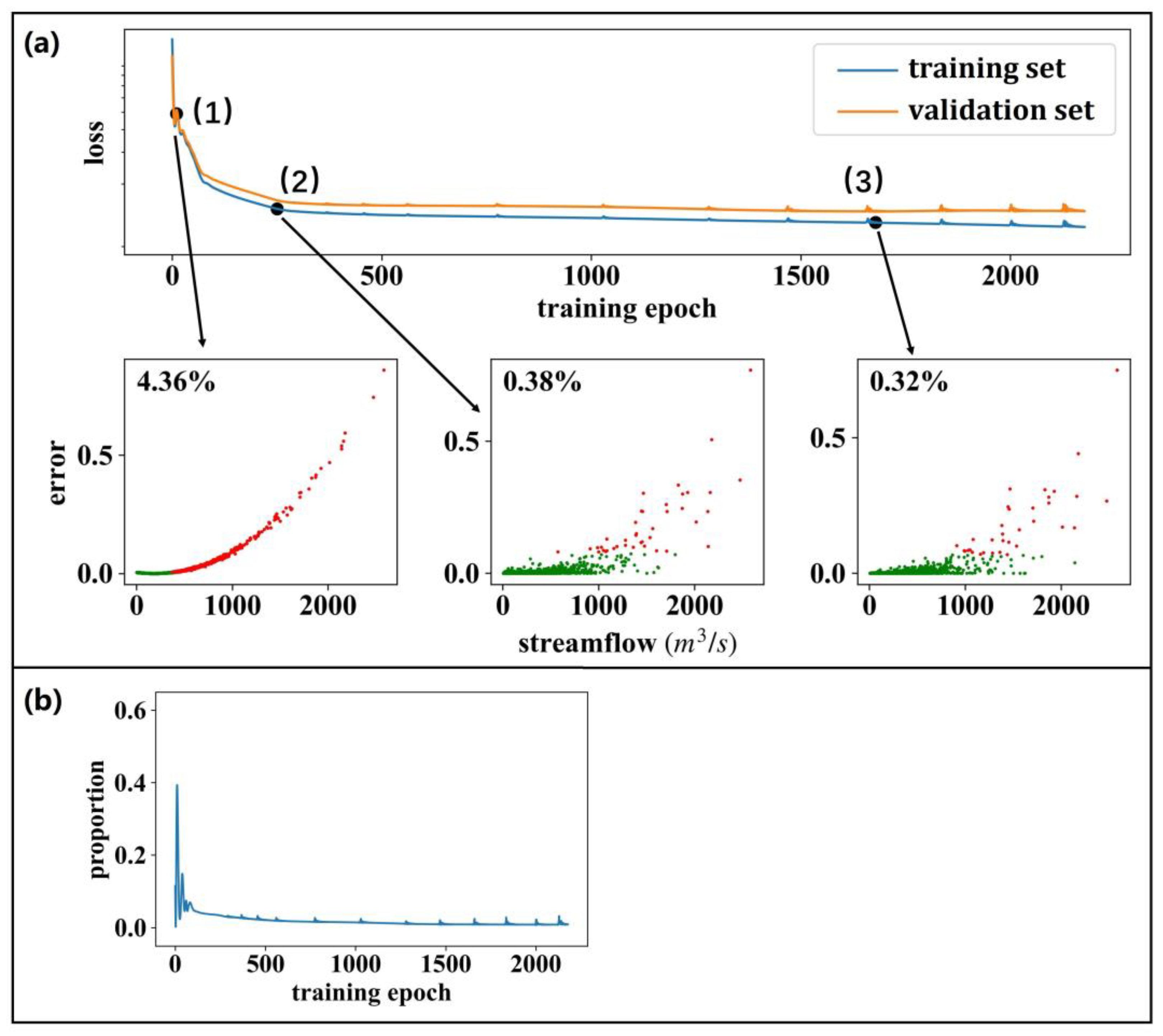
Figure 3 and Figure 4 clearly demonstrate that the models trained with squared-error-based objective functions are more skilled in high flow forecasting, but perform poorly in low flow forecasting. Here, we analyze the influence of training samples characterized by varying streamflow levels on the objective function in the model training process. Figure 6a displays the training process of an LSTM model that uses MSE as its objective function. We find that those training samples with higher streamflow values play a more important role in model training, since they contribute significantly more to the objective function. In the early stages of model training, only 4.36% of the training samples contribute 50% of the objective function, primarily concentrated in the area of high-value flows (the red dots in Figure 6a(1)). Subsequently, in the middle (Figure 6a(2)) and late (Figure 6a(3)) stages of the model training, this percentage drops to only 0.38% and 0.32%, respectively. This suggests that the model training process is heavily influenced by the high-value streamflow samples that only account for a small proportion of the total training samples. Figure 6b shows the contributions of the training samples with a streamflow within Q_0–0.5 bin on the objective function during the training of an LSTM model. It is evident that these samples exert a negligible effect, with their impact remaining below 0.05 during most of the training process, although they account for 50% of the total training samples.

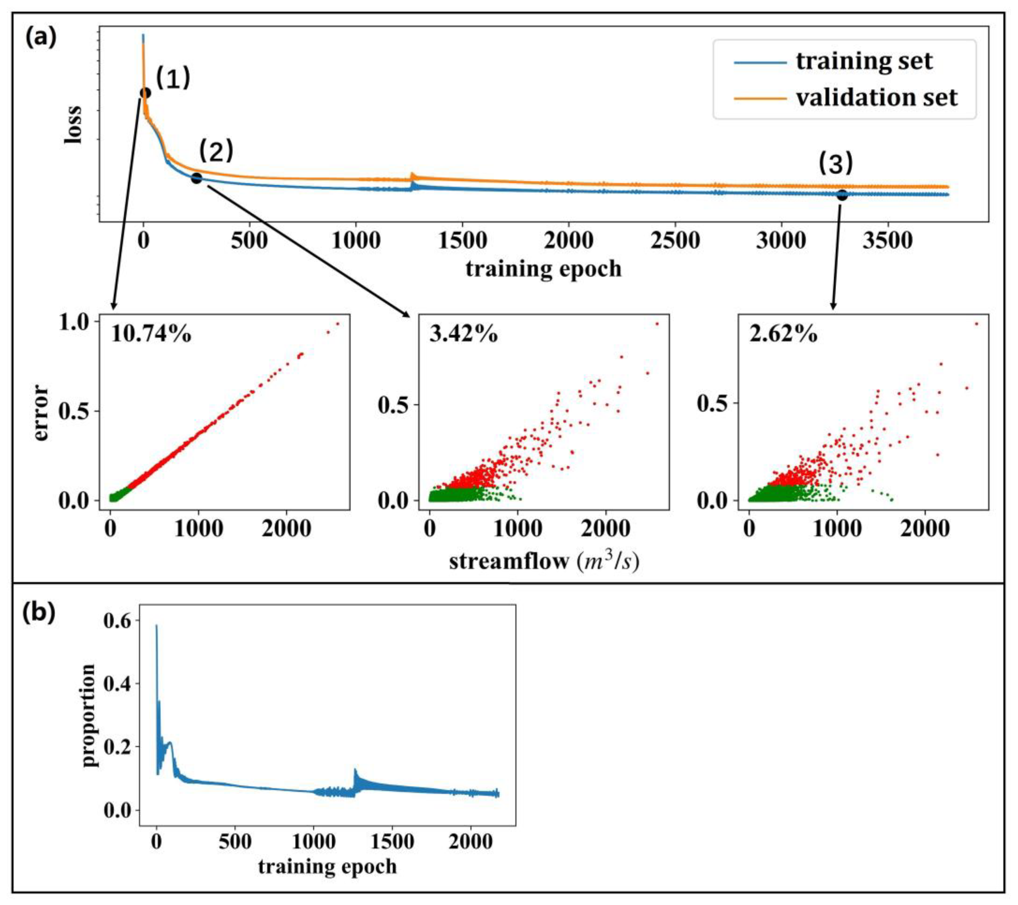
Figure 7a illustrates the training process of an LSTM when applying MAE as its objective function. Compared to using MSE for model training, when using MAE, the attention to the training samples is relatively less concentrated during the training process. In the early, middle, and late stages of model training, contributing 50% of the objective function requires 10.74%, 3.42%, and 2.62% of the training samples, respectively, which is a significant increase compared to using MSE as the objective function. In addition, samples with low or middle streamflow contribute more to the objective function (evidenced by the distribution of the red dots in Figure 7a(1)–(3)).

4.3. Assessment of Streamflow Modeling

4.3.1. Comparisons with a General Benchmark Method

The establishment of simple and universally applicable benchmark methods for hydrological modeling plays a crucial role in facilitating comparative assessments of diverse research outcomes. It also contributes to the robust and swift advancement of the hydrological modeling field. Currently, research on streamflow modeling is conducted by numerous independent groups, each primarily focused on developing and applying their own models and datasets. For various reasons, such as project requirements or limitations in computing resources, many researchers opt to utilize private, often small-scale streamflow datasets rather than accessing large publicly available ones, as seen in the works of Lee and Choi [48], Sun et al. [49], and Li et al. [50]. Additionally, given the varied technical backgrounds and time constraints of different researchers, it is impractical for them to explore all existing modeling methods with their individual datasets. Thus, the establishment of a simple, universal, and effective modeling method as a benchmark is a compelling necessity. Our recommended naïve method effectively addresses this need. By employing the naïve method as a benchmark, researchers can systematically evaluate the performance of their newly developed modeling techniques. This comparative approach enables them to gauge the degree of improvement (or potential deterioration) achieved by their proposed methodologies relative to the benchmark derived from the naïve method. Consequently, despite the differences in datasets across studies, this benchmarking process serves as an effective bridge connecting the results of these diverse investigations.

4.3.2. Evaluating Model Performance in Multiple Dimensions with Various Metrics

Evaluating modeling results through multiple metrics provides a comprehensive understanding of the strengths and limitations of newly proposed methods. Despite hydrologists introducing numerous evaluation metrics to measure modeling effectiveness, it is crucial to acknowledge that no single metric can fully cover the spectrum of modeling performance. Even comprehensive metrics like NSE and KGE have their limitations. For instance, NSE is more sensitive to high-flow errors, potentially resulting in satisfactory scores despite poor predictions for low flows. Therefore, adopting multiple metrics for assessing modeling results is of great significance.

Hydrologic signature metrics play a vital role in measuring hydrologic consistency, quantitatively describing statistical or dynamic properties of a hydrologic time series. These signatures encompass various aspects, including diurnal cycles, recession shapes, flow generation thresholds, rising limb density, baseflow index, runoff ratio, and flow variability. These metrics offer informative insights into the unique hydrologic processes of a watershed [51]. Utilizing multiple signature measures can provide a more comprehensive portrayal of hydrologic characteristics and a more realistic representation of various aspects of hydrologic processes [52]. Yilmaz et al. [51] also noted that hydrologic signatures have greater potential to delineate the temporal characteristics of river streamflow compared to the original streamflow time series.

Different facets of the hydrograph exhibit distinct characteristics, resulting in varying modeling effects for different parts of the hydrograph. Therefore, it is advisable to meticulously scrutinize the model’s performance across individual streamflow components. As demonstrated in Figure 3, our assessment of LSTM model performance is conducted with specific regard to varying streamflow levels. This analytical approach reveals a notable finding: the models demonstrate reduced efficacy for low flow forecasting. Such issues may be challenging to detect when evaluating the model’s performance based on the entire hydrograph.

5. Conclusions

In this study, we tested a simple and efficient benchmark method for short-term streamflow prediction, namely, the naïve method, which is applicable to almost all relevant research endeavors. Our experiment over 273 watersheds in the continental United States demonstrates that predictions from the naïve method can achieve acceptable or even excellent performance. Employing the naïve method as a benchmark can facilitate a more robust assessment of the strengths and weaknesses of newly proposed methods in research. Additionally, it fosters the inter-comparison of different research results, thereby promoting the healthy development of the field of hydrological modeling.

Through benchmarking with the naïve method, we identified a significant drawback in short-term streamflow forecasting models trained with squared-error-based objective functions, such as MSE and NSE. During the model training process, the objective function value is disproportionately influenced by errors in high-flow samples rather than low-flow samples when employing squared-error-based metrics. This disproportionate weight results in poor model performance in low-flow forecasting, sometimes even worse than the naïve method. Therefore, we advise against using squared-error-based metrics as the objective function for model training or calibration when the overall performance of streamflow prediction is the focus. Instead, we recommend using MAE as a more appropriate objective function. Additionally, in cases where process-based models are not employed, we suggest considering a pre-logarithmic transformation on the streamflow data. This step can help rectify the bias towards high-flow samples during model training, resulting in more balanced and reliable streamflow predictions.

In this study, we only assessed the performance of the naïve method on the GRDC dataset. In the future, we intend to apply the naïve method to other publicly available datasets, such as the CAMEL dataset. Additionally, we plan to evaluate the performance of more objective functions for the training of streamflow prediction models. Furthermore, while this study focused on evaluating a data-driven model, future research endeavors may broaden the evaluation scope to include physics-driven models.

References

- Karimizadeh, K.; Yi, J. Modeling Hydrological Responses of Watershed Under Climate Change Scenarios Using Machine Learning Techniques. Water Resour. Manag. 2023, preprint. [Google Scholar] [CrossRef]
- Zhou, J.; Wang, D.; Band, S.S.; Jun, C.; Bateni, S.M.; Moslehpour, M.; Pai, H.-T.; Hsu, C.-C.; Ameri, R. Monthly River Discharge Forecasting Using Hybrid Models Based on Extreme Gradient Boosting Coupled with Wavelet Theory and Lévy–Jaya Optimization Algorithm. Water Resour. Manag. 2023, 37, 3953–3972. [Google Scholar] [CrossRef]
- Bakhshi Ostadkalayeh, F.; Moradi, S.; Asadi, A.; Moghaddam Nia, A.; Taheri, S. Performance Improvement of LSTM-based Deep Learning Model for Streamflow Forecasting Using Kalman Filtering. Water Resour. Manag. 2023, 37, 3111–3127. [Google Scholar] [CrossRef]
- Sherman, L.K. Streamflow from rainfall by the unit-graph method. Eng. News Record 1932, 108, 501–505. [Google Scholar]
- Horton, R.E. Surface Runoff Phenomena. Part 1. Analysis of the Hydrograph. Horton Hydrologic Laboratory Publication 101. Edward Bros., Ann Arbor, Michigan. Horton Hydrol. Lab. 1935, 101. [Google Scholar]
- Penman, H.L.; Keen, B.A. Natural evaporation from open water, bare soil and grass. Proc. R. Soc. Lond. Ser. A Math. Phys. Sci. 1948, 193, 120–145. [Google Scholar]
- Sivapalan, M.; Takeuchi, K.; Franks, S.W.; Gupta, V.K.; Karambiri, H.; Lakshmi, V.; Liang, X.; Mcdonnell, J.J.; Mendiondo, E.M.; O’Connell, P.E.; et al. IAHS decade on predictions in ungauged basins (PUB), 2003–2012: Shaping an exciting future for the hydrological sciences. Hydrol. Sci. J. 2003, 48, 857–880. [Google Scholar] [CrossRef]
- Ren-Jun, Z. The Xinanjiang model applied in China. J. Hydrol. 1992, 135, 371–381. [Google Scholar] [CrossRef]
- Phien, H.N.; Pradhan, P. The tank model in rainfall-runoff modelling. Water SA 1983, 9, 93–102. [Google Scholar]
- Ragan, R.M.; Jackson, T.J. Runoff Synthesis Using Landsat and SCS Model. J. Hydraul. Div. 1980, 106, 667–678. [Google Scholar] [CrossRef]
- Sittner, W.T.; Schauss, C.E.; Monro, J.C. Continuous hydrograph synthesis with an API-type hydrologic model. Water Resour. Res. 1969, 5, 1007–1022. [Google Scholar] [CrossRef]
- Fang, L.; Huang, J.; Cai, J.; Nitivattananon, V. Hybrid approach for flood susceptibility assessment in a flood-prone mountainous catchment in China. J. Hydrol. 2022, 612, 128091. [Google Scholar] [CrossRef]
- Yang, J.; Wang, J.; Hu, Y.; Li, B.; Zhao, J.; Liang, Z. Flood risk mapping for the area with mixed floods and human impact: A case study of Yarkant River Basin in Xinjiang, China. Environ. Res. Commun. 2023, 5, 095005. [Google Scholar] [CrossRef]
- Chen, S.; Fu, Y.H.; Wu, Z.; Hao, F.; Hao, Z.; Guo, Y.; Geng, X.; Li, X.; Zhang, X.; Tang, J.; et al. Informing the SWAT model with remote sensing detected vegetation phenology for improved modeling of ecohydrological processes. J. Hydrol. 2023, 616, 128817. [Google Scholar] [CrossRef]
- Cerbelaud, A.; Lefèvre, J.; Genthon, P.; Menkes, C. Assessment of the WRF-Hydro uncoupled hydro-meteorological model on flashy watersheds of the Grande Terre tropical island of New Caledonia (South-West Pacific). J. Hydrol. Reg. Stud. 2022, 40, 101003. [Google Scholar] [CrossRef]
- Mostafa, R.R.; Kisi, O.; Adnan, R.M.; Sadeghifar, T.; Kuriqi, A. Modeling Potential Evapotranspiration by Improved Machine Learning Methods Using Limited Climatic Data. Water 2023, 15, 486. [Google Scholar] [CrossRef]
- Adnan, R.M.; Mostafa, R.R.; Dai, H.-L.; Heddam, S.; Kuriqi, A.; Kisi, O. Pan evaporation estimation by relevance vector machine tuned with new metaheuristic algorithms using limited climatic data. Eng. Appl. Comput. Fluid Mech. 2023, 17, 2192258. [Google Scholar] [CrossRef]
- Dorado-Guerra, D.Y.; Corzo-Pérez, G.; Paredes-Arquiola, J.; Pérez-Martín, M. Machine learning models to predict nitrate concentration in a river basin. Environ. Res. Commun. 2022, 4, 125012. [Google Scholar] [CrossRef]
- Madhushani, C.; Dananjaya, K.; Ekanayake, I.U.; Meddage, D.P.P.; Kantamaneni, K.; Rathnayake, U. Modeling streamflow in non-gauged watersheds with sparse data considering physiographic, dynamic climate, and anthropogenic factors using explainable soft computing techniques. J. Hydrol. 2024, 631, 130846. [Google Scholar] [CrossRef]
- Kratzert, F.; Klotz, D.; Herrnegger, M.; Sampson, A.K.; Hochreiter, S.; Nearing, G.S. Toward Improved Predictions in Ungauged Basins: Exploiting the Power of Machine Learning. Water Resour. Res. 2019, 55, 11344–11354. [Google Scholar] [CrossRef]
- Feng, D.; Fang, K.; Shen, C. Enhancing Streamflow Forecast and Extracting Insights Using Long-Short Term Memory Networks With Data Integration at Continental Scales. Water Resour. Res. 2020, 56, e2019WR026793. [Google Scholar] [CrossRef]
- Frame, J.M.; Kratzert, F.; Klotz, D.; Gauch, M.; Shalev, G.; Gilon, O.; Qualls, L.M.; Gupta, H.V.; Nearing, G.S. Deep learning rainfall–runoff predictions of extreme events. Hydrol. Earth Syst. Sci. 2022, 26, 3377–3392. [Google Scholar] [CrossRef]
- Frame, J.M.; Kratzert, F.; Raney, A.; Rahman, M.; Salas, F.R.; Nearing, G.S. Post-Processing the National Water Model with Long Short-Term Memory Networks for Streamflow Predictions and Model Diagnostics. JAWRA J. Am. Water Resour. Assoc. 2021, 57, 885–905. [Google Scholar] [CrossRef]
- Nearing, G.S.; Kratzert, F.; Sampson, A.K.; Pelissier, C.S.; Klotz, D.; Frame, J.M.; Prieto, C.; Gupta, H.V. What Role Does Hydrological Science Play in the Age of Machine Learning? Water Resour. Res. 2021, 57, e2020WR028091. [Google Scholar] [CrossRef]
- Mizukami, N.; Rakovec, O.; Newman, A.J.; Clark, M.P.; Wood, A.W.; Gupta, H.V.; Kumar, R. On the choice of calibration metrics for “high-flow” estimation using hydrologic models. Hydrol. Earth Syst. Sci. 2019, 23, 2601–2614. [Google Scholar] [CrossRef]
- Lin, Y.; Wang, D.; Zhu, J.; Sun, W.; Shen, C.; Shangguan, W. Development of objective function-based ensemble model for streamflow forecasts. J. Hydrol. 2024, 632, 130861. [Google Scholar] [CrossRef]
- Granata, F.; Di Nunno, F.; De Marinis, G. Stacked machine learning algorithms and bidirectional long short-term memory networks for multi-step ahead streamflow forecasting: A comparative study. J. Hydrol. 2022, 613, 128431. [Google Scholar] [CrossRef]
- Nash, J.E.; Sutcliffe, J.V. River flow forecasting through conceptual models part I—A discussion of principles. J. Hydrol. 1970, 10, 282–290. [Google Scholar] [CrossRef]
- Gupta, H.V.; Kling, H.; Yilmaz, K.K.; Martinez, G.F. Decomposition of the mean squared error and NSE performance criteria: Implications for improving hydrological modelling. J. Hydrol. 2009, 377, 80–91. [Google Scholar] [CrossRef]
- Kratzert, F.; Klotz, D.; Hochreiter, S.; Nearing, G.S. A note on leveraging synergy in multiple meteorological data sets with deep learning for rainfall–runoff modeling. Hydrol. Earth Syst. Sci. 2021, 25, 2685–2703. [Google Scholar] [CrossRef]
- Konapala, G.; Kao, S.-C.; Painter, S.L.; Lu, D. Machine learning assisted hybrid models can improve streamflow simulation in diverse catchments across the conterminous US. Environ. Res. Lett. 2020, 15, 104022. [Google Scholar] [CrossRef]
- Ghobadi, F.; Kang, D. Multi-Step Ahead Probabilistic Forecasting of Daily Streamflow Using Bayesian Deep Learning: A Multiple Case Study. Water 2022, 14, 3672. [Google Scholar] [CrossRef]
- Lin, Y.; Wang, D.; Wang, G.; Qiu, J.; Long, K.; Du, Y.; Xie, H.; Wei, Z.; Shangguan, W.; Dai, Y. A hybrid deep learning algorithm and its application to streamflow prediction. J. Hydrol. 2021, 601, 126636. [Google Scholar] [CrossRef]
- Kratzert, F.; Klotz, D.; Shalev, G.; Klambauer, G.; Hochreiter, S.; Nearing, G. Towards learning universal, regional, and local hydrological behaviors via machine learning applied to large-sample datasets. Hydrol. Earth Syst. Sci. 2019, 23, 5089–5110. [Google Scholar] [CrossRef]
- Kratzert, F.; Klotz, D.; Brenner, C.; Schulz, K.; Herrnegger, M. Rainfall–runoff modelling using Long Short-Term Memory (LSTM) networks. Hydrol. Earth Syst. Sci. 2018, 22, 6005–6022. [Google Scholar] [CrossRef]
- Hyndman, R.J.; Athanasopoulos, G. Forecasting: Principles and Practice; OTexts: Melbourne, Australia, 2013. [Google Scholar]
- Luo, R.; Wang, J.; Gates, I. Machine learning for accurate methane concentration predictions: Short-term training, long-term results. Environ. Res. Commun. 2023, 5, 081003. [Google Scholar] [CrossRef]
- Zhong, M.; Zhang, H.; Jiang, T.; Guo, J.; Zhu, J.; Wang, D.; Chen, X. A Hybrid Model Combining the Cama-Flood Model and Deep Learning Methods for Streamflow Prediction. Water Resour. Manag. 2023, 37, 4841–4859. [Google Scholar] [CrossRef]
- Vatanchi, S.M.; Etemadfard, H.; Maghrebi, M.F.; Shad, R. A Comparative Study on Forecasting of Long-term Daily Streamflow using ANN, ANFIS, BiLSTM and CNN-GRU-LSTM. Water Resour. Manag. 2023, 37, 4769–4785. [Google Scholar] [CrossRef]
- Sushanth, K.; Mishra, A.; Mukhopadhyay, P.; Singh, R. Real-time streamflow forecasting in a reservoir-regulated river basin using explainable machine learning and conceptual reservoir module. Sci. Total Environ. 2023, 861, 160680. [Google Scholar] [CrossRef]
- Lin, Y.; Wang, D.; Meng, Y.; Sun, W.; Qiu, J.; Shangguan, W.; Cai, J.; Kim, Y.; Dai, Y. Bias learning improves data driven models for streamflow prediction. J. Hydrol. Reg. Stud. 2023, 50, 101557. [Google Scholar] [CrossRef]
- Yuan, X.; Chen, C.; Lei, X.; Yuan, Y.; Muhammad Adnan, R. Monthly runoff forecasting based on LSTM–ALO model. Stoch. Environ. Res. Risk Assess. 2018, 32, 2199–2212. [Google Scholar] [CrossRef]
- Wang, Y.; Jian, Z.; Chen, K.; Wang, Y.; Liu, L. Water quality prediction method based on LSTM neural network. In Proceedings of the International Conference on Intelligent Systems & Knowledge Engineering 2017, Nanjing, China, 24–26 November 2017. [Google Scholar]
- Bowes, B.D.; Sadler, J.M.; Morsy, M.M.; Behl, M.; Goodall, J.L. Forecasting Groundwater Table in a Flood Prone Coastal City with Long Short-term Memory and Recurrent Neural Networks. Water 2019, 11, 1098. [Google Scholar] [CrossRef]
- Hochreiter, S.; Schmidhuber, J. Long Short-Term Memory. Neural Comput. 1997, 9, 1735–1780. [Google Scholar] [CrossRef] [PubMed]
- Lecun, Y.; Bengio, Y.; Hinton, G. Deep learning. Nature 2015, 521, 436–444. [Google Scholar] [CrossRef] [PubMed]
- Kingma, D.P.; Ba, J. Adam: A Method for Stochastic Optimization. arXiv 2014, arXiv:1412.6980. [Google Scholar]
- Lee, J.S.; Choi, H.I. A rebalanced performance criterion for hydrological model calibration. J. Hydrol. 2022, 606, 127372. [Google Scholar] [CrossRef]
- Sun, W.; Peng, T.; Luo, Y.; Zhang, C.; Hua, L.; Ji, C.; Ma, H. Hybrid short-term runoff prediction model based on optimal variational mode decomposition, improved Harris hawks algorithm and long short-term memory network. Environ. Res. Commun. 2022, 4, 045001. [Google Scholar] [CrossRef]
- Li, D.; Marshall, L.; Liang, Z.; Sharma, A.; Zhou, Y. Characterizing distributed hydrological model residual errors using a probabilistic long short-term memory network. J. Hydrol. 2021, 603, 126888. [Google Scholar] [CrossRef]
- Yilmaz, K.K.; Gupta, H.V.; Wagener, T. A process-based diagnostic approach to model evaluation: Application to the NWS distributed hydrologic model. Water Resour. Res. 2008, 44, W09417. [Google Scholar] [CrossRef]
- Mcmillan, H.K. A review of hydrologic signatures and their applications. WIREs Water 2020, 8, e1499. [Google Scholar] [CrossRef]
Figure 1.
The spatial distribution of 273 hydrological stations used in this study.
Figure 2.
The daily streamflow forecasting performance of the naïve method under different lead times for the (a) entire dataset, (b) training set, and (c) testing sets, respectively.
Figure 3.
Performance differences in terms of metrics MAPE, NSE, KGE, α, and β between the LSTM models trained with different objective functions and the naïve method with 1-day forecasting lead time in the testing set. The y-axis represents the evaluation metric values of LSTM minus the evaluation metric values of the naïve method. For the x-axis tick labels, “Q” stands for streamflow. The accompanying subscript number denotes the range of streamflow percentile in ascending order. To facilitate better comparison between different boxes, the y-axis range of the figures is limited, resulting in some boxes not being fully visible.
Figure 4.
The comparisons between the prediction evaluations of the LSTMMSE and that of the naïve method at different forecasting lead times for the (a) training set and (b) testing set, respectively.
Figure 5.
The relationship between the amplitude index (AI) of streamflow series and the forecasting performance of the naïve method. The numbers in the top-right corners represent the Pearson correlation coefficients.
Figure 6.
(a) The influence of different training samples on the model training process of an LSTM model with MSE as its objective function. The red dots denote the samples that contributed 50% of the objective function, while the green dots denote the remaining samples. (b) The proportion of the contributions of the training samples with a streamflow within Q0–0.5 bin on the training process of an LSTM model when applying MSE as the objective function.
Figure 7.
(a) The influence of different training samples on the model training process of an LSTM model with MAE as its objective function. The red dots denote the samples that contributed 50% of the objective function, while the green dots denote the remaining samples. (b) The proportion of the contributions of the training samples with a streamflow within Q0–0.5 bin on the training process of an LSTM model when applying MAE as the objective function.
Disclaimer/Publisher’s Note: The statements, opinions and data contained in all publications are solely those of the individual author(s) and contributor(s) and not of MDPI and/or the editor(s). MDPI and/or the editor(s) disclaim responsibility for any injury to people or property resulting from any ideas, methods, instructions or products referred to in the content. |
© 2024 by the authors. Licensee MDPI, Basel, Switzerland. This article is an open access article distributed under the terms and conditions of the Creative Commons Attribution (CC BY) license (https://creativecommons.org/licenses/by/4.0/).
Share and Cite
MDPI and ACS Style
Lin, Y.; Wang, D.; Jiang, T.; Kang, A. Assessing Objective Functions in Streamflow Prediction Model Training Based on the Naïve Method. Water 2024, 16, 777. https://doi.org/10.3390/w16050777
AMA Style
Lin Y, Wang D, Jiang T, Kang A. Assessing Objective Functions in Streamflow Prediction Model Training Based on the Naïve Method. Water. 2024; 16(5):777. https://doi.org/10.3390/w16050777
Chicago/Turabian StyleLin, Yongen, Dagang Wang, Tao Jiang, and Aiqing Kang. 2024. "Assessing Objective Functions in Streamflow Prediction Model Training Based on the Naïve Method" Water 16, no. 5: 777. https://doi.org/10.3390/w16050777
Note that from the first issue of 2016, this journal uses article numbers instead of page numbers. See further details here.