
Groundwater Temperature Stripes: A Simple Method to Communicate Groundwater Temperature Variations Due to Climate Change

Earth Sciences Department, University of Torino, 10125 Torin, Italy
*
Author to whom correspondence should be addressed.
Water 2024, 16(5), 717; https://doi.org/10.3390/w16050717
Submission received: 8 February 2024
/
Revised: 26 February 2024
/
Accepted: 26 February 2024
/
Published: 28 February 2024
(This article belongs to the Topic Effects of Climate Change on Geomorphology, Water Geochemistry and Pollution)
Abstract
:As our planet faces the complex challenges of global climate change, understanding and effectively communicating critical environmental indicators have become critical. This study explores the importance of reporting groundwater temperature data as a key component in understanding the broader implications of climate change with the use of new graphical tools. More specifically, the use of the groundwater temperature (GWT) stripes and bi-plots of GWT anomalies vs. time was proposed. For an in-depth examination of this subject, monitoring wells situated in the Piedmont Po plain (NW Italy) were selected, with available daily groundwater temperature data dating back to 2010. All data refer to the groundwater of the shallow unconfined aquifer within alluvial deposits. From the analyses of both GWT stripes and the bi-plot of GWT anomalies vs. time, it was possible to identify a general increase in the positive anomaly, corresponding to an increase in GWT in time in almost all of the monitoring points of the Piedmont plain. Furthermore, the utilisation of GWT stripes demonstrated the capability to effectively portray the trend of the GWT data relative to a specific point in a readily understandable manner, facilitating easy interpretation, especially when communicating to a non-scientific audience. The findings underline the urgent need to improve GWT data search and communication strategies to disseminate valuable information to policy makers, researchers, and society. By illustrating the intricate interplay between groundwater temperature and climate change, this research aims to facilitate informed decision-making and promote a proactive approach towards climate resilience.
1. Introduction
The discussion around climate change (CC) has gained popularity over the last 50 years; particularly in the last 10 years, the effects of CC have become increasingly evident (e.g., higher air temperature (AT), changing precipitation patterns, melting glaciers, and loss of biodiversity) [1]. In this context, the impacts of CC on water are becoming increasingly evident and have, at times, been catastrophic (e.g., floods and droughts).
However, there are consequences of CC that are not visible, but affect our lives in various aspects. Groundwater (GW), for example, is affected by CC, both qualitatively and quantitatively.
In the past, the impacts of CC on GW were analysed from a quantitative point of view, particularly by carrying out statistical analyses of trends in piezometric levels [2,3,4,5,6,7,8,9,10,11,12]; however, in recent years, there has been a growing focus on qualitative aspects, especially those related to GW temperature (GWT) variations [9,13,14,15,16,17,18,19,20,21,22,23,24,25,26,27,28,29,30,31].
In detail, GWT variations due to CC are of global interest and can be analysed from different perspectives, not only from a hydrogeological point of view, but also from the perspective of groundwater-dependent ecosystems [15,32,33,34,35,36,37,38,39,40,41] and potential industrial applications [18,42,43,44].
However, it is clear that the main vector for addressing this issue is the hydrogeological scientific community. Moreover, the hydrogeological community has the task of finding methods to communicate and disseminate scientific results to the civil population and stakeholders with decision-making power in the management of GW resources [45].
This mission is consistent with the motto chosen by the UN Water for World Water Day 2022, dedicated to GW, “Making the invisible visible” [46]. The aim of this initiative was to alert the scientific community and society to the issue of GW.
A similar procedure was used to evaluate the increase in AT due to CC. The most effective and communicative methods are the “warming stripes” (also known as “climate stripes”) by Ed Hawkins [47,48]. Warming stripes are an evolution of climate spirals from the same author [49]. The stripes are a graphic depiction of the AT fluctuations recorded in a country, a region, or a city over the course of the past century. More specifically, each stripe represents the average annual temperature anomaly at a specific location. Generally, climate stripe graphs start around the year 1900 and extend through 2022, although in numerous cases, they trace back to the 19th century or, occasionally, even the 18th century, depending on the availability of robust historical data. In most instances, the data are sourced from the Berkeley Earth temperature dataset [50], updated through the conclusion of 2022. However, for countries such as the USA, the UK, Switzerland, and Germany, data are obtained from their respective national meteorological agencies [51]. The colour scheme for each country’s stripes is established based on the average temperature during the period of 1971–2000, serving as the demarcation between the blue (cold) and red (hot) colours, with the white in between (0 value, no anomaly). Shades of blue indicate cooler-than-average temperature years, while red indicates years in which temperatures were hotter than the average. The colour scale of each representation encompasses a range of plus/minus 2.6 standard deviations relative to the annual average temperatures spanning 1901–2000 [51]. Regarding the global average, the UK Met Office HadCRUT5.0 dataset was utilised [52].
The use of warming stripes has become increasingly common to determine the impact of CC on AT. The simplicity of representation and interpretation, even for nonexperts, offered by warming stripes has made this method of communication a successful tool. For this reason, other disciplines have begun to use this methodology to highlight the impacts of CC on a given environmental matrix. In 2022, “Biodiversity Stripes” [53] were developed at the University of Derby based on the Living Planet Index (LPI) database [54]; these plants exhibited a decline in biodiversity between 1970 and 2018. In 2023, “Ocean Acidification Stripes” [55] were created at the ETH Zurich as a visual representation of the shift in ocean acidification in the past 40 years (1982–2022) based on the data product OceanSODA-ETHZ [56]. Both of these warming stripe-inspired methods are effective methods for graphically visualizing the impact of CC.
The purpose of this paper is to suggest new methods for identifying and communicating GWT variations due to CC. Specifically, the main aim is to graph this parameter in an easily and quickly interpretable way.
The first step was the proposal of a method borrowed from warming stripes called “groundwater temperature (GWT) stripes”. These stripes are intended to make visible one of the most important, but invisible, resources of our planet: GW. The advantages and weaknesses of this method were analysed and described. Moreover, a small study area, the Piedmont Po Plain, was chosen for testing the GWT stripes. As GWT data are not common, the choice was dictated by the availability of daily GWT measurements in this area since 2010 [57].
Study Area
The Piedmont region is situated in the northwestern part of Italy and covers an area of nearly 25,000 km2. Within the Piedmont region, the Po Plain accounts for approximately 27% of the entire region’s territory [58]. This plain is surrounded by the Alps to the north and east and the Apennines to the south.
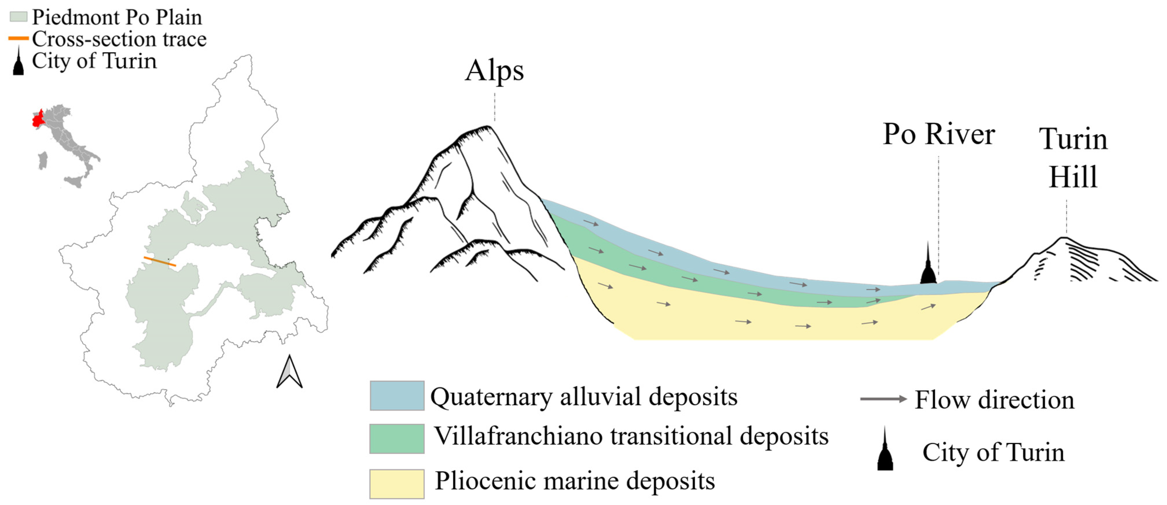
From a hydrogeological perspective, the Piedmont Po Plain consists of three hydrogeological units (Figure 1). Starting from the top, Quaternary alluvial deposits (lower Pleistocene-Holocene) hosting a shallow, unconfined aquifer are present. Below, Villafranchiano transitional deposits (late Pliocene–early Pleistocene) host a multilayered aquifer. Finally, Pliocene marine deposits (Pliocene) host a confined aquifer [58,59,60]. Due to its geological features and considerable size, the Piedmont Po Plain is recognized as the most significant groundwater reservoir in the Piedmont region [58].
In this study, we specifically focused on the shallow, unconfined aquifer located in the Piedmont Po Plain within Quaternary alluvial deposits. This aquifer has a thickness ranging from 20 to 50 m and is characterized by high hydraulic conductivity (K = 5 × 10⁻³–5 × 10⁻⁴ m/s); it primarily consists of coarse gravel and sand of fluvial or fluvioglacial origin, occasionally intermixed with silty clay layers [58]. The fluvial deposits are connected to the main rivers, particularly Po and Tanaro. At the base of the shallow aquifer, locally thick and continuous layers of silt or clay-rich deposits can be found, acting as the boundary between the shallow and the deeper aquifers [58].
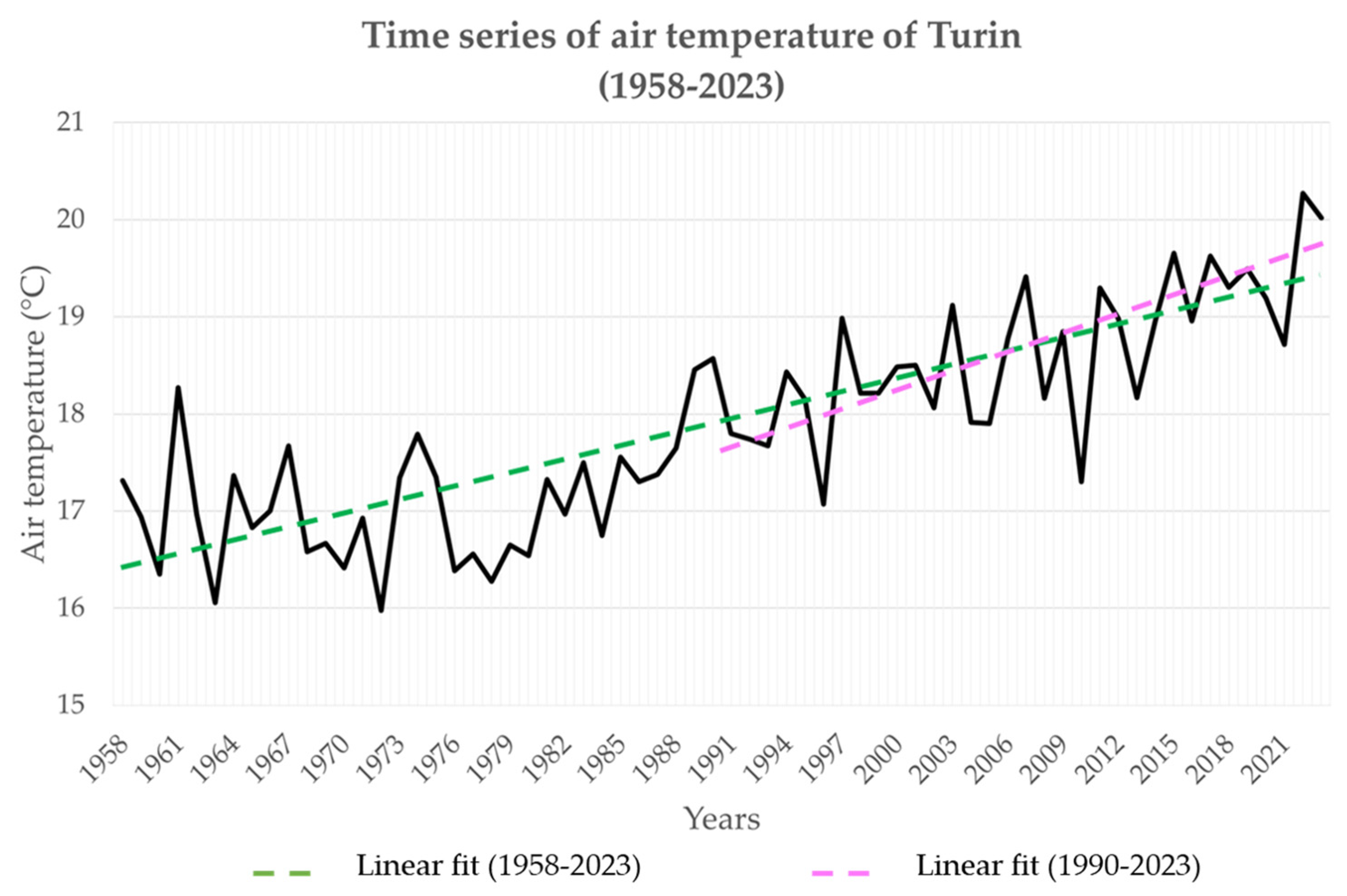
Regarding the climatic characteristics of the Piedmont mountains, the average annual AT decreases in a regular manner with altitude, with the exception of certain local conditions, such as urban areas where the temperature is slightly greater than that at the same altitude. In lowland plain areas, the average annual AT is between 10 and 12.5 °C [61,62]. By analysing long time series of AT data [23,63,64], starting in 1958, it is possible to highlight an increase in the average annual maximum AT of approximately 2.4 °C with a stronger positive trend in the last 30 years (Figure 2).
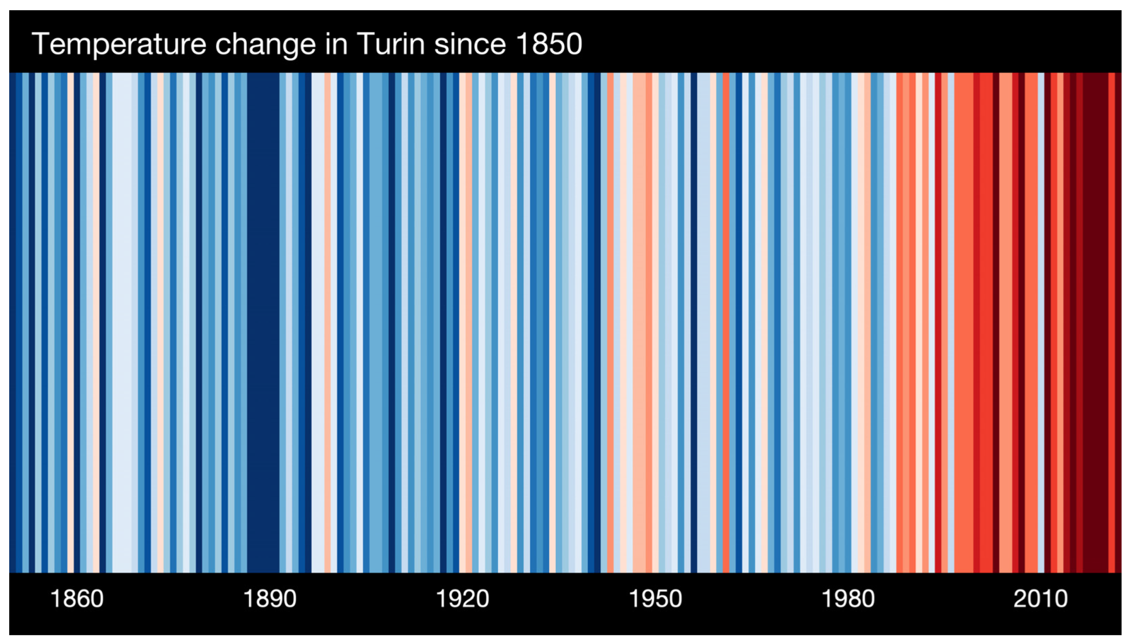
In addition, the Global Warming Stripes database [65], consulted for the city of Turin as the capital of the Piedmont Region, permitted the analysis of how the AT anomalies have varied since 1850 (Figure 3). Warming stripes highlight a clear increase in the anomaly value since 1990, confirming an increase in AT due to CC.
2. Materials and Methods
2.1. GWT Data
The data used for GWT stripe elaboration were daily GWTs. These data were measured by probes located in correspondence to the 139 monitoring wells of the Piedmont Po Plain automatic network managed by ARPA Piemonte, the regional Environmental Protection Agency. The main purpose of this network is to provide data, particularly on the quantitative status of the shallow aquifer. To do so, each monitoring well is equipped with an OTT Orpheus Mini, an integrated pressure sensor and datalogger for groundwater level measurements. However, the probe was also designed for the monitoring and storage of GWT data. Therefore, while the primary objective of this tool is to measure water levels, it is a valuable asset in searching for GWT data. GWT data, in fact, were typically not documented, particularly in the past, as they have only recently attracted scientific interest. The temperature sensor has a resolution of 0.1 °C and an accuracy of ±0.5 °C. OTT Orpheus Mini probes are generally positioned between 7 and 20 m from the topographic surface. Temperature data in the Piedmont Po Plain automatic network are available from January 2010 to December 2022 and are downloadable from the Regione Piemonte GREASE webpage [57]. Consequently, the analysed period covers an interval of 13 years.
The first step of the GWT data examination was screening analysis, in which historical series with less than 13 years of temperature data were deleted. The completeness index (CI) [66] was subsequently calculated according to the following equation (Equation (1)):
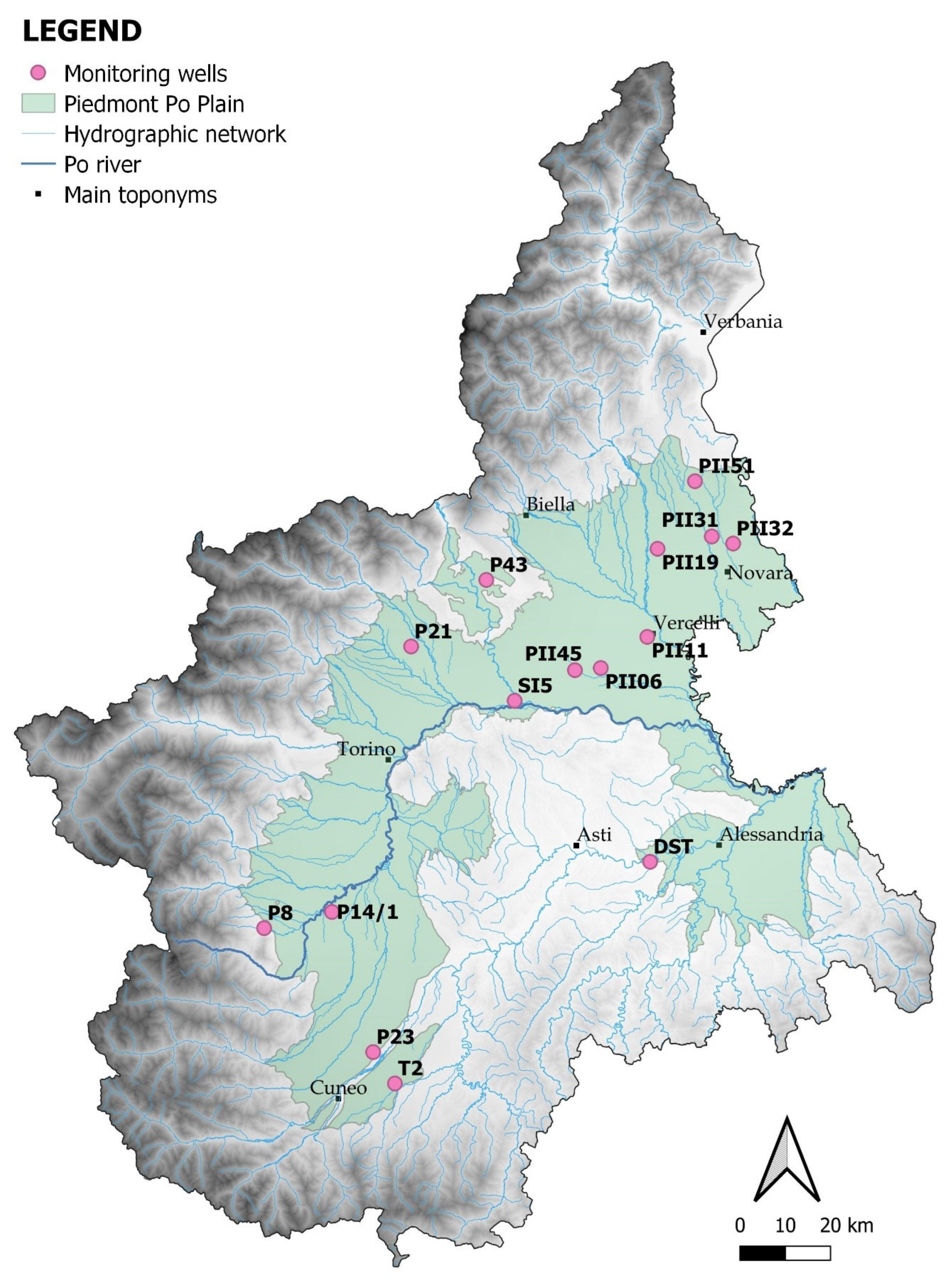
Monitoring wells with GWT measurement completeness greater than 90% over the period January 2010–December 2022 were chosen, for a total of 15 monitoring wells (Figure 4). The GWT data from these monitoring wells were then aggregated as monthly average values to observe the seasonality of the data over the chosen observation period.
The main features of the chosen monitoring wells (i.e., depth of the monitoring well, depth of the measuring instrument inside the monitoring well, distance between the topographical surface and the water table, and filtered intervals) are reported in Table 1. Indeed, previous studies show that the position of the instruments inside the monitoring well is crucial for the interpretation of temperature data [23]; more specifically, the closer the instrument is to the surface, the greater the sensitivity of the GWT data in relation to AT.
2.2. GWT Stripes Elaboration
To represent GWT data using GWT stripes, the monthly temperature anomaly (MTA) was calculated for each month of all analysed years.
In general, the anomaly (AN) was determined by calculating the difference between the annual (or monthly) values of a hydrological variable (X) and the mean values of the reference period (μXref) for the hydrological variable considered [67]. This calculation is expressed as (Equation (2)):
While AT annual data were used for the warming stripes, GWT monthly data were chosen for the GWT stripes. Indeed, the availability of GWT data is limited by a relatively short period of measurement; therefore, with annual data (in this case, 13 years), an accurate analysis could not be performed. Furthermore, the use of monthly data also allows the seasonality of the data to be observed in the final graphical output.
To represent GWT data using GWT stripes, MTA was calculated for each month of all analysed years, as follows (Equation (3)):
For example, for January 2010, the MTA was calculated as follows (Equation (4)):
Once all the anomaly values for all months were calculated in the analysed period (13 years), a total of 156 values were available to create GWT stripes for each monitoring well.
While warming stripe data are represented by blue, white, and red [68], GWT stripe data are represented by light blue to orange. The chosen colour scale indicates the lowest negative value of the anomaly in deep blue and the highest positive value of the anomaly in deep orange; white indicates stationarity in the parameter (no anomaly). As was the case for the warming stripes, the scale colour of the GWT stripes represents a GWT increase when warm colours are used, and the GWT decreases when cold colours are used.
Because of the modality of GWT stripe elaboration (Equation (3)), the scale colour is typical of each location and each historical series, and a colour will not necessarily correspond to the same temperature anomaly in other locations. The data were used to construct a schematic representation of the Piedmont region: cold and hot colours represent negative and positive annual anomalies, respectively. This approach does not allow for a comparison of the GWT stripes.
To compare the anomalies in the monitoring wells of the study area, data were also organized in column graphs, in which the abscissa shows the time and the ordinate the anomaly value.
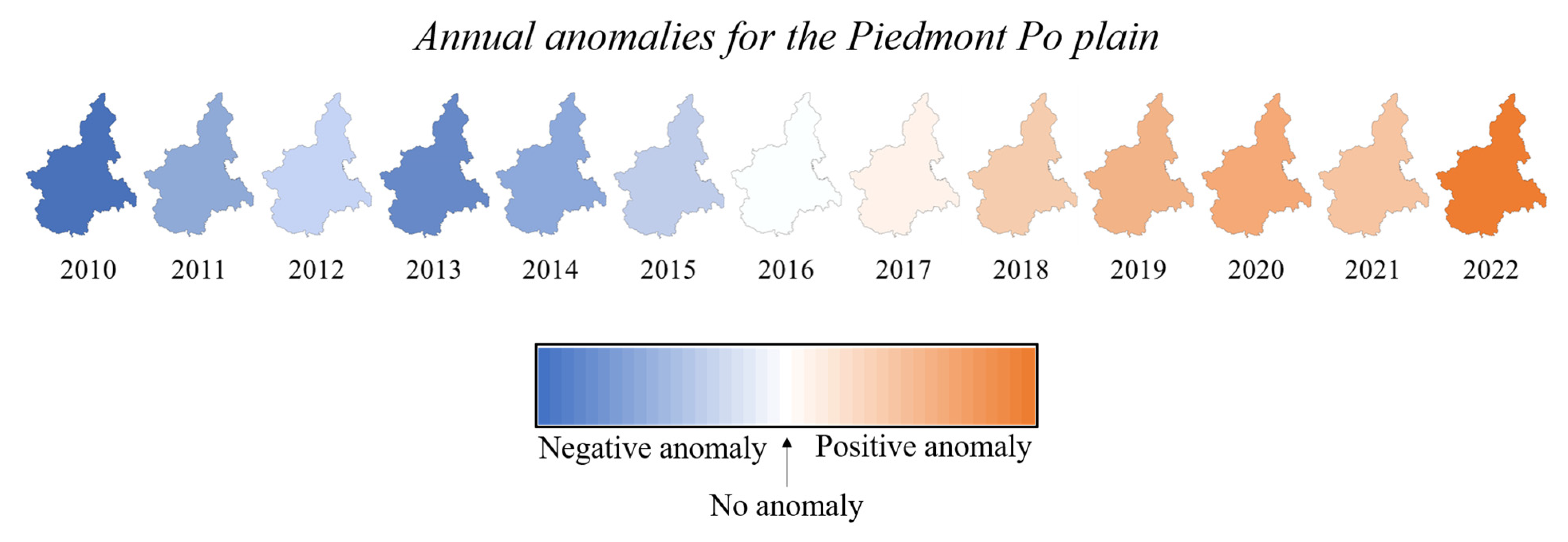
Finally, in order to provide an overview of the GWT increase on a regional scale, a representation of the annual GWT anomalies was proposed for the entire Piedmont Po Valley. The anomaly data of the 15 regionally distributed points was averaged into a single value. The GWT anomaly for each year analysed was calculated as the average of each monthly anomaly for each year. This provides a unique value for each year, which allows for the creation of an easy-to-use graphic representation for dissemination purposes.
3. Results
Once all GWT data had been processed for all 15 monitoring wells, two graphical representations were produced that could be used alone or in pairs to provide a clearer picture of GWT variations over the observed time period:
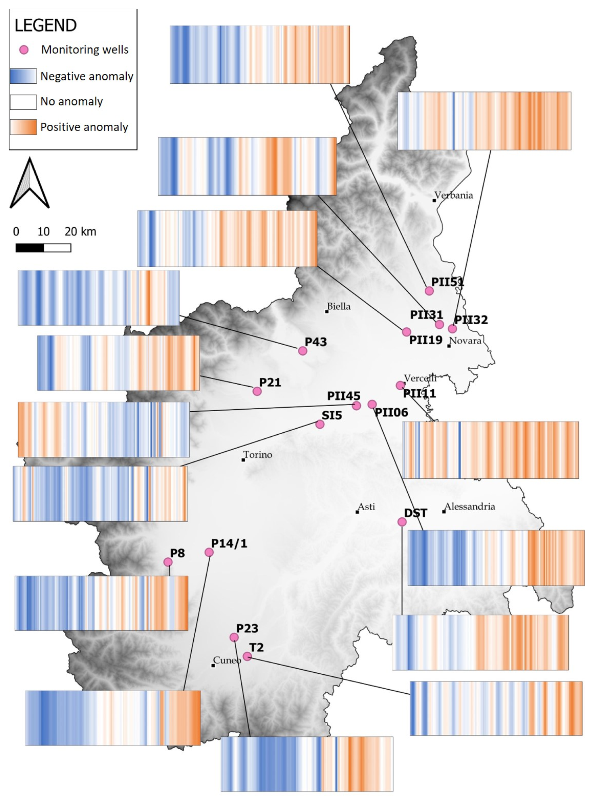
- A map of Piedmont with the GWT stripes for each monitoring well, allowing an immediate evaluation of the GWT trend in the specific piezometer (Figure 5);
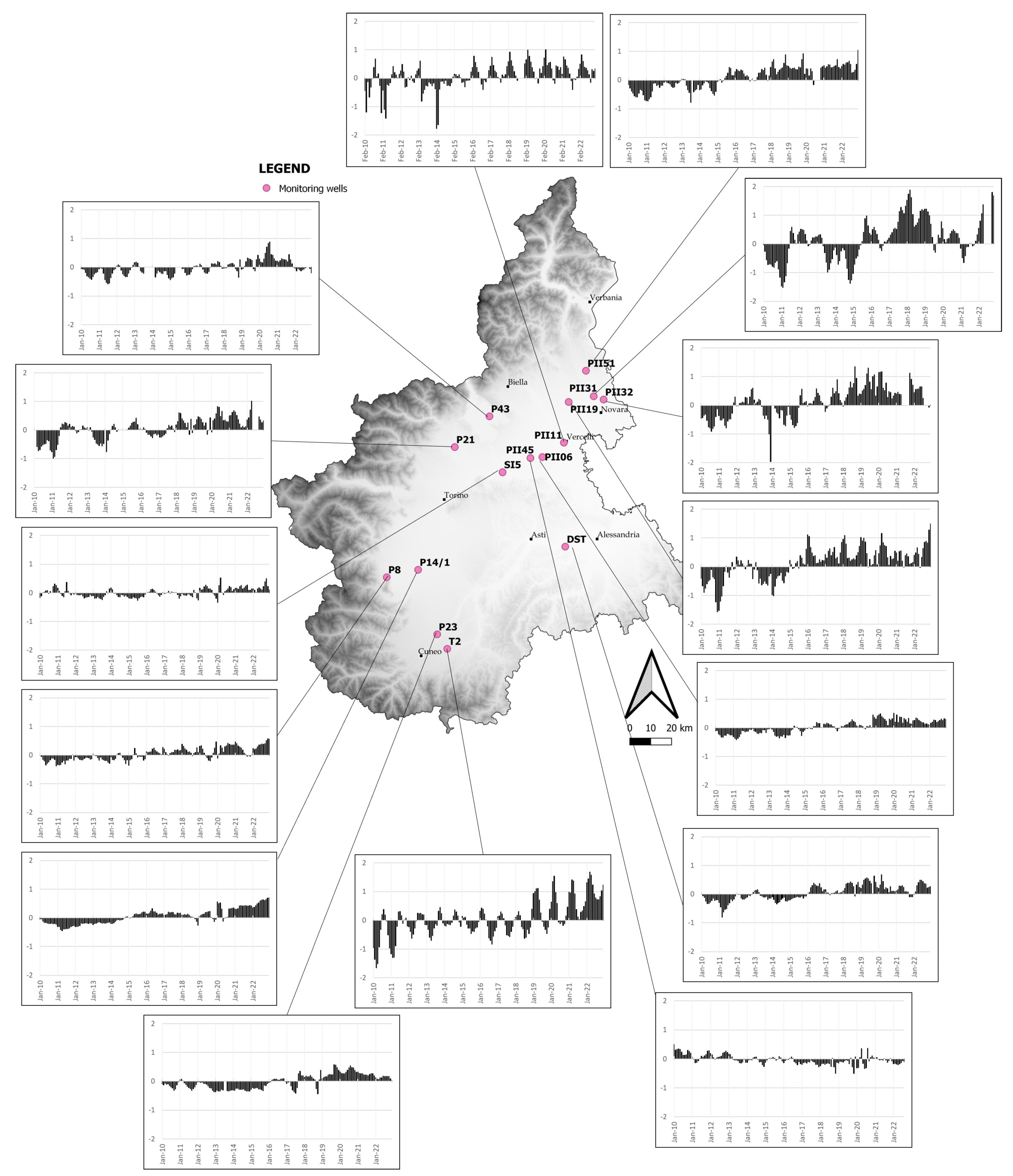
- A map of Piedmont with column graphs, using the same scale, for all 15 monitoring wells, allowing a graphical comparison of GWT data between all the analysed piezometers (Figure 6).
In both figures, it can be observed that, in 14 of the 15 analysed monitoring wells (PII11, PII19, PII31, PII32, T2, PII51, P43, P21, SI5, P8, P14/1, DST, P23, and PII06), there was an increase in the positive anomaly, corresponding to an increase in the GWT. In Figure 3, the increase in the positive anomaly is represented by the predominance of orange bands in recent years. However, GWT stripes do not indicate the magnitude of the anomaly (positive or negative).
To assess the magnitude of the anomalies, Figure 6 uses the same vertical scale on the ordinate axis (axis of anomaly); with this type of analysis, it can be highlighted that, despite the general upwards temperature trend highlighted in Figure 5 represented by the positive anomaly, in monitoring wells PII11, PII19, PII31, PII32, and T2, there was a particularly noticeable increase in positive anomalies (even more than 1 °C).
In the other monitoring wells (PII51, P43, P21, SI5, P8, P14/1, DST, P23, and PII06), a generally positive anomaly in recent years could be highlighted; however, these wells had values less than 1 °C.
Furthermore, this representation allowed us to report the year that marks the passage from a negative to a positive anomaly, generally in the interval of 2015–2016. Only one piezometer, PII45, located in Trino (Vercelli Province), showed a decrease in anomalies in recent years, which could be observed both in Figure 5 and Figure 6 and was linked to a decrease in GWT over the observed time period. The magnitude of the anomaly (Figure 6) was very small, generally less than 0.3 °C.
Finally, Figure 7 provides an overview of the annual GWT anomaly on a regional scale. While this constitutes a representation of a value averaged across the 15 analysed points and subsequently averaged to a single annual figure, it is apparent that there was a rise in GWT at the regional level over the 13 years analysed, notably commencing in 2016.
4. Discussion and Conclusions
The aim of this paper was to identify an easy-to-interpret graphical method for visualizing GWT variations in a CC context.
To determine which was the best method to achieve this goal, real GWT data that could be statistically processed were searched. Specifically, GWT data from monitoring wells on the Piedmont Po Plain (NW Italy) were obtained. GWT data were analysed with GWT stripes and a biplot of the monthly GWT anomaly in the period of 2010–2022. In particular, the GWT stripe method for the representation of GWT anomalies was borrowed from the warming stripe method and was used for other parameters, such as AT, loss of biodiversity, and ocean acidification. The warming stripes strategy has been proven to be effective for communication not only directed toward the scientific community, but also, and above all, toward the general public.
From the analyses of both GWT stripes and biplots of GWT anomalies vs. time, it was possible to identify a general increase in the positive anomaly, corresponding to an increase in GWT over time at almost all of the monitoring points on the Piedmont Plain. This outcome is justified by the increase in AT observed in Piedmont [23,63]. However, as also observed in previous work [23], the increasing trend for AT was more pronounced than that for GWT; consequently, it is possible to state that GWTs are more resilient to change than ATs.
Only one piezometer, PII45, showed a decrease in anomalies in recent years, linked to a decrease in GWT over the observed time period. This piezometer was located within an industrial area where there was a thermoelectric power plant. For this reason, interpreting these results was difficult since they could be connected to the impact of anthropogenic activities carried out on the surface rather than to the impact of CC. For this reason, the data from these monitoring points will be further analysed in future studies to better understand their different behaviours compared with those of the other monitoring wells in the Piedmont Plain.
The use of GWT stripes demonstrated the ability to effectively portray the trend of the GWT data relative to a specific point in a readily understandable manner, facilitating easy interpretation. Nonetheless, a drawback associated with GWT stripes is that, despite employing a consistent colour scale within a given region, each stripe’s representation is contingent upon the values of the analysed point. Moreover, GWT stripes did not indicate the magnitude of the anomaly, positive or negative; consequently, they did not facilitate the correlation of data between two distinct points.
Owing to this consideration, biplots of GWT anomalies vs. time were also generated using a uniform scale across the entire study area. This approach was adopted to facilitate the comparative analysis of all the monitored wells with greater ease. The main result of this study was an absolute increase in the GWT in the analysed period, with anomaly values in some cases also being higher than +2 °C.
Furthermore, the use of monthly anomalies in the GWT, both for GWT stripes and biplots, was proven to be effective for visualizing the seasonality of the data. Consequently, it was possible to observe that, in most cases, an increase in the GWT anomaly occurred during both the summer and winter seasons. This outcome was not possible using only the annual average anomaly (as for the warming stripes).
Finally, the utilization of monthly anomalies served as an advantageous strategy for highlighting trends in short historical series. Indeed, in the Piedmont Plain case study, the annual average anomaly for the period 2010–2022 in each monitoring well yielded only 13 stripes. However, employing monthly anomalies allowed for the creation of 156 bands, providing a more comprehensive mean for assessing the variation in anomalies.
The approach of using both GWT stripes and biplots of anomalies vs. time permitted us to highlight that stripes are the best way to communicate the issue of GWT changes due to CC to society. This approach is straightforward and expeditious for disseminating the issue of groundwater warming.
The analysis of data for scientists and stakeholders, however, should also be paired with other representations, such as biplots, to better analyse the magnitude of the GWT change.
It is evident that the lack of data on GWT was the main problem for its representation. Indeed, the longest time series are usually used for statistical analysis, i.e., for air temperature studies; however, data regarding the groundwater temperature are generally limited because they have historically garnered little interest among scientists. Only recently has there been a start in collecting and analysing them.
In the future, it is imperative to establish databases focused on groundwater temperatures that facilitate regional, national, and even global research endeavours. Having comparable data across various scales will undoubtedly be the most effective approach to enhancing public awareness of the issue, aiming for improved resource management.
Author Contributions
Conceptualization, E.E. and M.L.; formal analysis: E.E. and M.L.; Methodology: E.E. and M.L.; data curation, E.E. and M.L.; writing—original draft preparation, E.E. and M.L.; writing—review and editing, E.E. and M.L.; supervision, D.A.D.L. All authors have read and agreed to the published version of the manuscript.
Funding
This research received no external funding.
Data Availability Statement
Data are contained within the article.
Acknowledgments
The authors would like to thank Fiorella Acquaotta for her help in climate data interpretation.
Conflicts of Interest
The authors declare no conflicts of interest.
Abbreviations
| AN | anomaly |
| AT | air temperatre |
| CC | climate change |
| GW | groundwater |
| GWT | groundwater temperature |
| MTA | monthly temperature anomaly |
References
- Pörtner, H.-O.; Roberts, D.C.; Tignor, M.; Poloczanska, E.S.; Mintenbeck, K.; Alegría, A.; Craig, M.; Langsdorf, S.; Löschke, S.; Möller, V.; et al. IPCC 2022: Climate Change 2022: Impacts, Adaptation and Vulnerability. Contribution of Working Group II to the Sixth Assessment Report of the Intergovernmental Panel on Climate Change; Cambridge University Press: Cambridge, UK, 2022; Volume 3056. [Google Scholar] [CrossRef]
- Dragoni, W.; Sukhija, B.S. Climate Change and Groundwater: A Short Review. Geol. Soc. Lond. Spec. Publ. 2008, 288, 1–12. [Google Scholar] [CrossRef]
- Egidio, E.; Lasagna, M.; Mancini, S.; Luca, D.A.D. Climate Impact Assessment to the Groundwater Levels Based on Long Time-Series Analysis in a Paddy Field Area (Piedmont Region, NW Italy): Preliminary Results. Acque Sotter. Ital. J. Groundw. Acque Sotter. 2022, 3, 21–29. [Google Scholar] [CrossRef]
- Holman, I.P. Climate Change Impacts on Groundwater Recharge-Uncertainty, Shortcomings, and the Way Forward? Hydrogeol. J. 2006, 14, 637–647. [Google Scholar] [CrossRef]
- Jasechko, S.; Seybold, H.; Perrone, D.; Fan, Y.; Shamsudduha, M.; Taylor, R.G.; Fallatah, O.; Kirchner, J.W. Rapid Groundwater Decline and Some Cases of Recovery in Aquifers Globally. Nature 2024, 625, 715–721. [Google Scholar] [CrossRef]
- Kjellström, E.; Nikulin, G.; Strandberg, G.; Christensen, O.B.; Jacob, D.; Keuler, K.; Lenderink, G.; van Meijgaard, E.; Schär, C.; Somot, S.; et al. European Climate Change at Global Mean Temperature Increases of 1.5 and 2 °C above Pre-Industrial Conditions as Simulated by the EURO-CORDEX Regional Climate Models. Earth Syst. Dynam. 2018, 9, 459–478. [Google Scholar] [CrossRef]
- Lasagna, M.; Mancini, S.; De Luca, D.A. Groundwater Hydrodynamic Behaviours Based on Water Table Levels to Identify Natural and Anthropic Controlling Factors in the Piedmont Plain (Italy). Sci. Total Environ. 2020, 716, 137051. [Google Scholar] [CrossRef]
- Taniguchi, M. Evaluation of Vertical Groundwater Fluxes and Thermal Properties of Aquifers Based on Transient Temperature-Depth Profiles. Water Resour. Res. 1993, 29, 2021–2026. [Google Scholar] [CrossRef]
- Taylor, C.A.; Stefan, H.G. Shallow Groundwater Temperature Response to Climate Change and Urbanization. J. Hydrol. 2009, 375, 601–612. [Google Scholar] [CrossRef]
- Doll, P.; Fiedler, K. Global-Scale Modeling of Groundwater Recharge. Hydrol. Earth Syst. Sci. 2008, 12, 863–885. [Google Scholar] [CrossRef]
- Khan, S.; Gabriel, H.F.; Rana, T. Standard Precipitation Index to Track Drought and Assess Impact of Rainfall on Watertables in Irrigation Areas. Irrig. Drain. Syst. 2008, 22, 159–177. [Google Scholar] [CrossRef]
- Scanlon, B.R.; Keese, K.E.; Flint, A.L.; Flint, L.E.; Gaye, C.B.; Edmunds, W.M.; Simmers, I. Global Synthesis of Groundwater Recharge in Semiarid and Arid Regions. Hydrol. Process. 2006, 20, 3335–3370. [Google Scholar] [CrossRef]
- Bastiancich, L.; Lasagna, M.; Mancini, S.; Falco, M.; De Luca, D.A. Temperature and Discharge Variations in Natural Mineral Water Springs Due to Climate Variability: A Case Study in the Piedmont Alps (NW Italy). Env. Geochem. Health 2021, 44, 1971–1994. [Google Scholar] [CrossRef] [PubMed]
- Benz, S.; Bayer, P.; Blum, P. Global Patterns of Shallow Groundwater Temperatures. Environ. Res. Lett. 2017, 12, 034005. [Google Scholar] [CrossRef]
- Burns, E.R.; Zhu, Y.; Zhan, H.; Manga, M.; Williams, C.F.; Ingebritsen, S.E.; Dunham, J.B. Thermal Effect of Climate Change on Groundwater-Fed Ecosystems. Water Resour. Res. 2017, 53, 3341–3351. [Google Scholar] [CrossRef]
- Epting, J.; Michel, A.; Affolter, A.; Huggenberger, P. Climate Change Effects on Groundwater Recharge and Temperatures in Swiss Alluvial Aquifers. J. Hydrol. X 2021, 11, 100071. [Google Scholar] [CrossRef]
- Gunawardhana, L.N.; Kazama, S. Climate Change Impacts on Groundwater Temperature Change in the Sendai Plain, Japan. Hydrol. Process. 2011, 25, 2665–2678. [Google Scholar] [CrossRef]
- Hemmerle, H.; Bayer, P. Climate Change Yields Groundwater Warming in Bavaria, Germany. Front. Earth Sci. 2020, 8, 575894. [Google Scholar] [CrossRef]
- Kurylyk, B.L.; MacQuarrie, K.T.B.; Caissie, D.; McKenzie, J.M. Shallow Groundwater Thermal Sensitivity to Climate Change and Land Cover Disturbances: Derivation of Analytical Expressions and Implications for Stream Temperature Modeling. Hydrol. Earth Syst. Sci. 2015, 19, 2469–2489. [Google Scholar] [CrossRef]
- Kurylyk, B.L.; MacQuarrie, K.T.B.; Voss, C.I. Climate Change Impacts on the Temperature and Magnitude of Groundwater Discharge from Shallow, Unconfined Aquifers. Water Resour. Res. 2014, 50, 3253–3274. [Google Scholar] [CrossRef]
- Menberg, K.; Blum, P.; Kurylyk, B.L.; Bayer, P. Observed Groundwater Temperature Response to Recent Climate Change. Hydrol. Earth Syst. Sci. 2014, 18, 4453–4466. [Google Scholar] [CrossRef]
- Noethen, M.; Hemmerle, H.; Bayer, P. Sources, Intensities, and Implications of Subsurface Warming in Times of Climate Change. Crit. Rev. Environ. Sci. Technol. 2022, 53, 700–722. [Google Scholar] [CrossRef]
- Egidio, E.; Mancini, S.; De Luca, D.A.; Lasagna, M. The Impact of Climate Change on Groundwater Temperature of the Piedmont Po Plain (NW Italy). Water 2022, 14, 2797. [Google Scholar] [CrossRef]
- Blanco-Coronas, A.M.; Calvache, M.L.; López-Chicano, M.; Martín-Montañés, C.; Jiménez-Sánchez, J.; Duque, C. Salinity and Temperature Variations near the Freshwater-Saltwater Interface in Coastal Aquifers Induced by Ocean Tides and Changes in Recharge. Water 2022, 14, 2807. [Google Scholar] [CrossRef]
- Cogswell, C.; Heiss, J.W. Climate and Seasonal Temperature Controls on Biogeochemical Transformations in Unconfined Coastal Aquifers. JGR Biogeosciences 2021, 126, e2021JG006605. [Google Scholar] [CrossRef]
- Irvine, D.J.; Kurylyk, B.L.; Cartwright, I.; Bonham, M.; Post, V.E.A.; Banks, E.W.; Simmons, C.T. Groundwater Flow Estimation Using Temperature-Depth Profiles in a Complex Environment and a Changing Climate. Sci. Total Environ. 2017, 574, 272–281. [Google Scholar] [CrossRef]
- Mastrocicco, M.; Busico, G.; Colombani, N. Groundwater Temperature Trend as a Proxy for Climate Variability. Proceedings 2018, 2, 630. [Google Scholar] [CrossRef]
- Mastrocicco, M.; Busico, G.; Colombani, N. Deciphering Interannual Temperature Variations in Springs of the Campania Region (Italy). Water 2019, 11, 288. [Google Scholar] [CrossRef]
- Cavelan, A.; Golfier, F.; Colombano, S.; Davarzani, H.; Deparis, J.; Faure, P. A Critical Review of the Influence of Groundwater Level Fluctuations and Temperature on LNAPL Contaminations in the Context of Climate Change. Sci. Total Environ. 2022, 806, 150412. [Google Scholar] [CrossRef]
- Lee, B.; Hamm, S.-Y.; Jang, S.; Cheong, J.-Y.; Kim, G.-B. Relationship between Groundwater and Climate Change in South Korea. Geosci. J. 2014, 18, 209–218. [Google Scholar] [CrossRef]
- Colombani, N.; Giambastiani, B.M.S.; Mastrocicco, M. Use of Shallow Groundwater Temperature Profiles to Infer Climate and Land Use Change: Interpretation and Measurement Challenges. Hydrol. Process. 2016, 30, 2512–2524. [Google Scholar] [CrossRef]
- Danielopol, D.L.; Griebler, C.; Gunatilaka, A.; Notenboom, J. Present State and Future Prospects for Groundwater Ecosystems. Envir. Conserv. 2003, 30, 104–130. [Google Scholar] [CrossRef]
- Kløve, B.; Ala-Aho, P.; Bertrand, G.; Gurdak, J.J.; Kupfersberger, H.; Kværner, J.; Muotka, T.; Mykrä, H.; Preda, E.; Rossi, P.; et al. Climate Change Impacts on Groundwater and Dependent Ecosystems. J. Hydrol. 2014, 518, 250–266. [Google Scholar] [CrossRef]
- Lomeli-Banda, M.A.; Ramírez-Hernández, J.; Rodríguez-Burgueño, J.E.; Salazar-Briones, C. The Role of Hydrological Processes in Ecosystem Conservation: Comprehensive Water Management for a Wetland in an Arid Climate. Hydrol. Process. 2021, 35, e14013. [Google Scholar] [CrossRef]
- Colloff, M.J.; Baldwin, D.S. Resilience of Floodplain Ecosystems in a Semi-Arid Environment. Rangel. J. 2010, 32, 305. [Google Scholar] [CrossRef]
- Brielmann, H.; Griebler, C.; Schmidt, S.I.; Michel, R.; Lueders, T. Effects of Thermal Energy Discharge on Shallow Groundwater Ecosystems: Ecosystem Impacts of Groundwater Heat Discharge. FEMS Microbiol. Ecol. 2009, 68, 273–286. [Google Scholar] [CrossRef]
- Rivers-Moore, N.A.; Dallas, H.F. A Spatial Freshwater Thermal Resilience Landscape for Informing Conservation Planning and Climate Change Adaptation Strategies. Aquat. Conserv. Mar. Freshw. Ecosyst. 2022, 32, 832–842. [Google Scholar] [CrossRef]
- Johnson, Z.C.; Snyder, C.D.; Hitt, N.P. Landform Features and Seasonal Precipitation Predict Shallow Groundwater Influence on Temperature in Headwater Streams. Water Resour. Res. 2017, 53, 5788–5812. [Google Scholar] [CrossRef]
- Morsy, K.M.; Alenezi, A.; AlRukaibi, D.S. Groundwater and Dependent Ecosystems: Revealing the Impacts of Climate Change. Int. J. Appl. Eng. Res. 2017, 12, 3919–3926. [Google Scholar]
- Carlson, A.K.; Taylor, W.W.; Infante, D.M. Developing Precipitation- and Groundwater-Corrected Stream Temperature Models to Improve Brook Charr Management amid Climate Change. Hydrobiologia 2019, 840, 379–398. [Google Scholar] [CrossRef]
- Fan, M.; Shibata, H.; Chen, L. Spatial Priority Conservation Areas for Water Yield Ecosystem Service under Climate Changes in Teshio Watershed, Northernmost Japan. J. Water Clim. Change 2020, 11, 106–129. [Google Scholar] [CrossRef]
- Epting, J.; Huggenberger, P. Unraveling the Heat Island Effect Observed in Urban Groundwater Bodies—Definition of a Potential Natural State. J. Hydrol. 2013, 501, 193–204. [Google Scholar] [CrossRef]
- Fennell, J.; Geris, J.; Wilkinson, M.E.; Daalmans, R.; Soulsby, C. Lessons from the 2018 Drought for Management of Local Water Supplies in Upland Areas: A Tracer-Based Assessment. Hydrol. Process. 2020, 34, 4190–4210. [Google Scholar] [CrossRef]
- Berta, A.; Gizzi, M.; Taddia, G.; Lo Russo, S. The Role of Standards and Regulations in the Open-Loop GWHPs Development in Italy: The Case Study of the Lombardy and Piedmont Regions. Renew. Energy 2024, 223, 120016. [Google Scholar] [CrossRef]
- Petitta, M.; Kreamer, D.; Davey, I.; Dottridge, J.; MacDonald, A.; Re, V.; Szőcs, T. Topical Collection: International Year of Groundwater—Managing Future Societal and Environmental Challenges. Hydrogeol. J. 2023, 31, 1–6. [Google Scholar] [CrossRef] [PubMed]
- United Nations. Groundwater Making the Invisible Visible; UN Water, Ed.; The United Nations World Water Development Report; UNESCO: Paris, France, 2022; ISBN 978-92-3-100507-7. [Google Scholar]
- Warming Stripes|Climate Lab Book. Available online: https://www.climate-lab-book.ac.uk/warming-stripes/ (accessed on 26 July 2023).
- Show Your Stripes. Available online: https://showyourstripes.info/ (accessed on 22 July 2023).
- Climate Spirals|Climate Lab Book. Available online: https://www.climate-lab-book.ac.uk/spirals/ (accessed on 2 October 2023).
- Environmental Science, Data, and Analysis of the Highest Quality Independent, Non-Governmental, and Open-Source. Available online: https://berkeleyearth.wpengine.com/ (accessed on 3 October 2023).
- Hawkins, E. Show Your Stripes. Available online: https://showyourstripes.info/faq (accessed on 3 October 2023).
- Morice, C.P.; Kennedy, J.J.; Rayner, N.A.; Winn, J.P.; Hogan, E.; Killick, R.E.; Dunn, R.J.H.; Osborn, T.J.; Jones, P.D.; Simpson, I.R. An Updated Assessment of Near-Surface Temperature Change From 1850: The HadCRUT5 Data Set. JGR Atmos. 2021, 126, e2019JD032361. [Google Scholar] [CrossRef]
- Richardson, M. #BiodiversityStripes. Available online: https://biodiversitystripes.info/ukfarmlandbirds/landscape (accessed on 26 July 2023).
- Living Planet Index. Available online: https://www.livingplanetindex.org/ (accessed on 3 October 2023).
- Gruber, N.; Gregor, L. #AcidificationStripes. Available online: https://oceanacidificationstripes.info/s/ph/basin/globalocean/entirebasin (accessed on 2 October 2023).
- Gregor, L.; Gruber, N. OceanSODA-ETHZ: A Global Gridded Data Set of the Surface Ocean Carbonate System for Seasonal to Decadal Studies of Ocean Acidification. Earth Syst. Sci. Data 2021, 13, 777–808. [Google Scholar] [CrossRef]
- Regione Piemonte GREASE. Available online: https://webgis.arpa.piemonte.it/monitoraggio_qualita_acque_mapseries/monitoraggio_qualita_acque_webapp/ (accessed on 14 September 2023).
- De Luca, D.A.; Lasagna, M.; Debernardi, L. Hydrogeology of the Western Po Plain (Piedmont, NW Italy). J. Maps 2020, 16, 265–273. [Google Scholar] [CrossRef]
- Cocca, D.; Lasagna, M.; Marchina, C.; Brombin, V.; Santillán Quiroga, L.M.; De Luca, D.A. Assessment of the Groundwater Recharge Processes of a Shallow and Deep Aquifer System (Maggiore Valley, Northwest Italy): A Hydrogeochemical and Isotopic Approach. Hydrogeol. J. 2023. [Google Scholar] [CrossRef]
- Forno, M.G.; De Luca, D.A.; Festa, V.; Bonasera, M.; Bucci, A.; Gianotti, F.; Lasagna, M.; Longhitano, S.G.; Lucchesi, S.; Petruzzelli, M.; et al. Synthesis on the Turin Subsoil Stratigraphy and Hydrogeology (NW Italy). AMQ 2018, 31, 1–24. [Google Scholar] [CrossRef]
- Bucci, A.; Barbero, D.; Lasagna, M.; Forno, M.G.; De Luca, D.A. Shallow Groundwater Temperature in the Turin Area (NW Italy): Vertical Distribution and Anthropogenic Effects. Environ. Earth. Sci. 2017, 76, 221. [Google Scholar] [CrossRef]
- Bucci, A.; Lasagna, M.; De Luca, D.A.; Acquaotta, F.; Barbero, D.; Fratianni, S. Time Series Analysis of Underground Temperature and Evaluation of Thermal Properties in a Test Site of the Po Plain (NW Italy). Environ. Earth. Sci. 2020, 79, 185. [Google Scholar] [CrossRef]
- Brussolo, E.; Palazzi, E.; von Hardenberg, J.; Masetti, G.; Vivaldo, G.; Previati, M.; Canone, D.; Gisolo, D.; Bevilacqua, I.; Provenzale, A.; et al. Aquifer Recharge in the Piedmont Alpine Zone: Historical Trends and Future Scenarios. Hydrol. Earth Syst. Sci. 2022, 26, 407–427. [Google Scholar] [CrossRef]
- Arpa Piemonte Stazione: Torino—Serie Ultracentenarie—Dati Dal 1787. Available online: https://www.arpa.piemonte.it/rischi_naturali/snippets_arpa_graphs/dati_giornalieri_centenaria/?statid=PIE-001272-100-1787-01-01¶m=T (accessed on 7 February 2024).
- Hawkins, E. Show Your Stripes Turin. Available online: https://showyourstripes.info/l/europe/italy/turin (accessed on 7 February 2024).
- Braca, G.; Bussettini, M.; Lastoria, B.; Mariani, S. Linee Guida per l’analisi e l’elaborazione Statistica di Base delle Serie Storiche di Dati Idrologici; Guidelines n. 84/2013; ISPRA: Rome, Italy, 2013; ISBN 978-88-448-0584-5.
- Mancini, S.; Egidio, E.; De Luca, D.A.; Lasagna, M. Application and Comparison of Different Statistical Methods for the Analysis of Groundwater Levels over Time: Response to Rainfall and Resource Evolution in the Piedmont Plain (NW Italy). Sci. Total Environ. 2022, 846, 157479. [Google Scholar] [CrossRef] [PubMed]
- Climate Stripes—University of Reading. Available online: https://www.reading.ac.uk/planet/climate-resources/climate-stripes (accessed on 26 July 2023).
Figure 1.
Sketch of a cross-section of the hydrogeological units of the Po Plain. The red line highlights the localization of the cross-section.
Figure 1.
Sketch of a cross-section of the hydrogeological units of the Po Plain. The red line highlights the localization of the cross-section.

Figure 2.
Time series of annual average air temperature data for the city of Turin for the period of 1958–2023. Dashed coloured lines represent the linear fit for different time periods: green 1958–2023; pink: 1990–2023.
Figure 2.
Time series of annual average air temperature data for the city of Turin for the period of 1958–2023. Dashed coloured lines represent the linear fit for different time periods: green 1958–2023; pink: 1990–2023.

Figure 3.
Warming stripes for the city of Turin for the period of 1850–2022 downloaded from [65]. The air temperature anomaly was calculated over the period 1971–2000.
Figure 3.
Warming stripes for the city of Turin for the period of 1850–2022 downloaded from [65]. The air temperature anomaly was calculated over the period 1971–2000.

Figure 4.
Map with localization of the 15 chosen monitoring wells.

Figure 5.
Regional map with GWT stripes allowing an immediate evaluation of the GWT trend in the analysed monitoring wells. GWT data refer to the period of 2010–2022.
Figure 5.
Regional map with GWT stripes allowing an immediate evaluation of the GWT trend in the analysed monitoring wells. GWT data refer to the period of 2010–2022.

Figure 6.
Regional map with the biplot of monthly GWT anomaly in the period of 2010–2022, allowing a comparison of the magnitude of GWT variation for the 15 analysed monitoring wells.
Figure 6.
Regional map with the biplot of monthly GWT anomaly in the period of 2010–2022, allowing a comparison of the magnitude of GWT variation for the 15 analysed monitoring wells.

Figure 7.
Graphic representation of the annual groundwater temperature (GWT) anomalies for the entire Piedmont Po Plain. The anomaly data of the 15 regionally distributed points was averaged into a single value.
Figure 7.
Graphic representation of the annual groundwater temperature (GWT) anomalies for the entire Piedmont Po Plain. The anomaly data of the 15 regionally distributed points was averaged into a single value.


Table 1.
Main features of monitoring wells.
| Monitoring Well | Location | X Coordinate (WGS 84, UTM 32) | Y Coordinate (WGS 84, UTM 32) | Altitude (m a.s.l.) | Depth of the Monitoring Well (m) | Depth of the Instrument (m) | Distance Between the Topographic Surface and the Water Table (m) | Filtered Interval (m) |
|---|---|---|---|---|---|---|---|---|
| PII51 | Suno | 463753 | 5053032 | 251 | 15 | 10 | 4.87 | 6–15 |
| PII31 | Caltignaga | 467448 | 5040801 | 179 | 15 | 15 | 3.73 | 6–15 |
| PII32 | Cameri | 472183 | 5039246 | 164 | 15 | 15 | 4.92 | 6–15 |
| PII19 | Landiona | 455465 | 5038163 | 180 | 15 | 15 | 1.67 | 3–15 |
| P43 | Albiano d’Ivrea | 417580 | 5031184 | 229 | 24 | 11.4 | 4.08 | 12–24 |
| PII11 | Vercelli | 453187 | 5018583 | 131 | 35 | 10 | 3.56 | 3–15 |
| PII06 | Ronsecco | 442911 | 5011693 | 145 | 25 | 10 | 4.06 | 9–15 |
| PII45 | Trino | 437139 | 5011305 | 156 | 15 | 15 | 3.2 | 3–15 |
| P21 | Rivarolo Canavese | 400961 | 5016462 | 266 | 20 | 15 | 3.47 | 11–20 |
| SI5 | Verolengo | 423853 | 5004449 | 177 | 18 | 15 | 9.84 | 5–20 |
| P8 | Barge | 368435 | 4954232 | 335 | 39 | 20 | 10.18 | 18–39 |
| P14/1 | Moretta | 383530 | 4957900 | 252 | 30 | 10 | 2.14 | 12–30 |
| P23 | Fossano | 392537 | 4926862 | 412 | 30 | 20 | 10.16 | 15–30 |
| T2 | Morozzo | 397367 | 4919953 | 430 | 30 | 10 | 3.76 | 5–11 |
| DST | Masio | 453833 | 4968900 | 101 | 8 | 8 | 4.81 | 0–8 |
Disclaimer/Publisher’s Note: The statements, opinions and data contained in all publications are solely those of the individual author(s) and contributor(s) and not of MDPI and/or the editor(s). MDPI and/or the editor(s) disclaim responsibility for any injury to people or property resulting from any ideas, methods, instructions or products referred to in the content. |
© 2024 by the authors. Licensee MDPI, Basel, Switzerland. This article is an open access article distributed under the terms and conditions of the Creative Commons Attribution (CC BY) license (https://creativecommons.org/licenses/by/4.0/).
Share and Cite
MDPI and ACS Style
Lasagna, M.; Egidio, E.; De Luca, D.A. Groundwater Temperature Stripes: A Simple Method to Communicate Groundwater Temperature Variations Due to Climate Change. Water 2024, 16, 717. https://doi.org/10.3390/w16050717
AMA Style
Lasagna M, Egidio E, De Luca DA. Groundwater Temperature Stripes: A Simple Method to Communicate Groundwater Temperature Variations Due to Climate Change. Water. 2024; 16(5):717. https://doi.org/10.3390/w16050717
Chicago/Turabian StyleLasagna, Manuela, Elena Egidio, and Domenico Antonio De Luca. 2024. "Groundwater Temperature Stripes: A Simple Method to Communicate Groundwater Temperature Variations Due to Climate Change" Water 16, no. 5: 717. https://doi.org/10.3390/w16050717
Note that from the first issue of 2016, this journal uses article numbers instead of page numbers. See further details here.