
Monthly Streamflow Prediction of the Source Region of the Yellow River Based on Long Short-Term Memory Considering Different Lagged Months
1
College of Architecture and Civil Engineering, Beijing University of Technology, Beijing 100124, China
2
Chinese Research Academy of Environmental Sciences, Beijing 100012, China
*
Author to whom correspondence should be addressed.
Water 2024, 16(4), 593; https://doi.org/10.3390/w16040593
Submission received: 14 January 2024
/
Revised: 9 February 2024
/
Accepted: 9 February 2024
/
Published: 17 February 2024
(This article belongs to the Section Hydrology)
Abstract
:Accurate and reliable monthly streamflow prediction plays a crucial role in the scientific allocation and efficient utilization of water resources. In this paper, we proposed a prediction framework that integrates the input variable selection method and Long Short-Term Memory (LSTM). The input selection methods, including autocorrelation function (ACF), partial autocorrelation function (PACF), and time lag cross-correlation (TLCC), were used to analyze the lagged time between variables. Then, the performance of the LSTM model was compared with three other traditional methods. The framework was used to predict monthly streamflow at the Jimai, Maqu, and Tangnaihai stations in the source area of the Yellow River. The results indicated that grid search and cross-validation can improve the efficiency of determining model parameters. The models incorporating ACF, PACF, and TLCC with lagged time are evidently superior to the models using the current variable as the model inputs. Furthermore, the LSTM model, which considers the lagged time, demonstrated better performance in predicting monthly streamflow. The coefficient of determination (R2) improved by an average of 17.46%, 33.94%, and 15.29% for each station, respectively. The integrated framework shows promise in enhancing the accuracy of monthly streamflow prediction, thereby aiding in strategic decision-making for water resources management.
1. Introduction
Streamflow plays an important role in the process of the management of water supply, hydropower generation, and ecological preservation. The previous studies demonstrated that 77% of rivers show no notable changes in annual water flow, while 11% have experienced a decrease. Decreased streamflow is mainly observed in central and western Africa, eastern Asia, southern Europe, western North America, and eastern Australia. For instance, since 1948, the flow in the Pacific Northwest has significantly decreased in low-flow years. River discharge in the Bakırçay River basin, Huangfuchuan basin of the Yellow River, Kocabaş stream of Turkey, and the Euphrates–Tigris basin all clearly demonstrated a declining tendency. In contrast, 12% of rivers increased their annual flow. Increased streamflow is predominantly found in northern Asia, northern Europe, and northern and eastern North America as global warming intensifies the hydrological cycle. These dynamics are driven by trends in climate forcing, cryosphere response to warming, and human water management [1,2]. In 2022, an average surface water resource of approximately 2.60 × 10¹² m3 was recorded in China. The Yellow River, the second largest river in China, which supports 12% of the population and 15% of its irrigated land, has experienced significant streamflow fluctuations during the last six decades. It fell into decline and dried up in the late twentieth century, but it has since recovered and stabilized. It is crucial to comprehend the future trends of the Yellow River, particularly its source area, water resource planning, and taking measures for drought or floods in advance [3].
Accurate streamflow prediction is significant to water resources planning and management, as well as for the early warning and alleviation of natural hazards such as drought and flood [4]. The Qinghai-Tibet Plateau is an initiator and amplifier of the global climate, and the streamflow in its basin has received more and more attention in terms of both the evolution mechanism and the future magnitude. The source region of the Yellow River (SAYR) which is located in the interior of the Qinghai-Tibet Plateau is an important source of fresh water in China, accounting for 38% of the total annual flow of the Yellow River, and it is crucial for water resource in northwest China [5,6]. Therefore, it is vital to predict streamflow in the SAYR for a better understanding of the availability and management of streamflow.
Many streamflow prediction methods developed in the past are mainly divided into physical models and data-driven models [7,8,9]. It is dilemmatic to establish an accurate prediction model because the physical model is based on the physical process and needs to accurately describe the flow process and the streamflow data has non-stationary, non-linear, and large spatiotemporal variability [10,11]. In addition, strict data requirements also limit the application of the model in large basins [12]. On the contrary, the data-driven models can predict the streamflow at a certain time more efficiently and accurately by mining the evolution characteristics of the streamflow generation process through historical climate and streamflow data [13,14,15]. Various data-driven models have been developed for streamflow prediction, such as machine learning and deep learning including Support Vector Machines (SVM) [16,17], Generalized Regression Neural Network (GRNN) [18], Deep Neural Network (DNN) [19], Recurrent Neural Network (RNN) [20,21], Long Short-Term Memory (LSTM) [22,23]. Among them, LSTM, as a variant model of RNN, has a more prominent application effect in hydrology. Hu et al. [24] used ANN and LSTM network models to simulate the rainfall–runoff process in the flood season of the Fen River Basin. The results show that both of these two networks are suitable for the rainfall–runoff model and are better than the conceptual and physics-based models, while the R2 and NSE values of the LSTM model are more than 0.9 respectively, which is better than the ANN model. Kratzert et al. [25] show that the strength of LSTM is its ability to learn long-term dependencies between inputs and outputs provided by the network and use 241 catchment areas as tests, demonstrating the potential of LSTM in hydrological modeling applications. Ding et al. [26] proposed an explainable spatiotemporal attentional Long short-term memory model (STA-LSTM) based on LSTM and attention mechanism to meet the needs of flood prediction. The experimental results in three small and medium river basins in China show that the STA-LSTM model is superior to other models in most cases. Song et al. [27] proposed a flood prediction model (LSTM-FF) based on LSTM, the research shows that the LSTM-FF model can effectively predict flash floods, especially the qualification rate of large-scale flood events.
Although the potential of LSTM in time series prediction has been proved in many studies [28,29], the influence of input and parameter setting on prediction accuracy in monthly streamflow needs further study. When the lagged time is small, some effective information will be missed from the training sets, and if the lagged time is too large, it not only increases the complexity of the model but also retains the interference information [30]. Therefore, it is very crucial to determine the lagged time of input variables efficiently to improve the prediction accuracy. Three methods, including autocorrelation function (ACF), partial autocorrelation function (PACF), and time lag cross-correlation (TLCC), are often used to comprehensively analyze the lagged time of input variables. TLCC is used to measure the lag relationship between different variables, and ACF and PACF are used to measure the autocorrelation of the variable. Through these approaches, the most favorable input combination of the model can be found and then used to develop a superior adaptive prediction model [31].
Parameter setting in data-driven models is a critical process of model development [32]. If the parameter selection is not appropriate, the problem of underfitting or overfitting will appear. There are two methods for parameter determination. One way is that the parameters are manually adjusted according to the experience, which is time-consuming and inefficient. The other is that different parameters can be adjusted within the specified interval, and the parameters with the highest accuracy are found from all the parameters by training, and then the optimal parameters are further determined through cross-validation, such as grid search and cross-validation, GridSearchCV.
The purpose of this paper is as follows: (1) to determine the lagged time of input variables including meteorological variables and previous streamflow on current streamflow, (2) to study the potential of LSTM model in monthly streamflow prediction and the optimal parameters for three hydrological stations in the source area of the Yellow River, and (3) to compare the performance of LSTM with other models and evaluate the influence of the lagged time of input variables on model performance. In this paper, a prediction framework is proposed that integrates the lagged time of input variables method and LSTM models, and three stations including Jimai, Maqu, and Tangnaihai in the source area of the Yellow River were used as case studies. Finally, the performance of the LSTM model is compared with those of three other models and the influence of the lagged time of input variables on model performance was evaluated.
2. Method
This study aimed to determine the lag time of each factor by considering runoff and meteorological factors. Based on this, the study conducted subsequent comparative modeling of multiple prediction models and evaluated the prediction results. The factors influencing runoff include meteorological conditions and previous runoff patterns. Therefore, the ACF and PACF were used for a comprehensive analysis of the time lag between the current runoff and the previous runoff. Additionally, the TLCC was used to analyze the lag time between current runoff and historical meteorological factors, as well as current meteorological factors, in order to determine the input data for the model at different times. The model performance can be affected by an excessive or insufficient number of input variables.
2.1. Long Short-Term Memory (LSTM)
LSTM is an enhanced architecture developed from recurrent neural networks (RNN) [33,34], which aims to learn and predict time series data. LSTM has a similar chain structure to the traditional RNN, but the LSTM unit introduces cell state and three gate structures to maintain and control information, which makes the internal operation of LSTM more complex [35,36]. Compared with RNN, the subtlety of LSTM is that it uses gated units to replace neurons in the hidden layer of RNN so that it can selectively “remember” and “forget” the information in the long time series to avoid the gradient disappearance and explosion problems of RNN, and then use backpropagation algorithm to update the hyperparameters and optimize the model to make its model prediction result more accurate [37,38,39]. In the structure of LSTM, the hidden layer of the LSTM neural network contains forget gate (), input gate (), output gate () and memory unit () [40]. Among them, the forget gate is used to determine the amount of information discarded in the previous memory unit. The input gate is used to determine the proportion of current information input into the memory unit. The output gate is used to determine the output information at the current moment. This process is mathematically shown in the following six equations [41,42]:
where is the state of the temporary memory unit at time ; represents the final output calculated by the function represents the function; represents the output of the previous cell; represents the input of the current cell; represents the hyperbolic tangent activation function; , , , and represent the weight matrices from the hidden layer to the forget gate, input gate, memory unit, and output gate, respectively; and , , , and represent the bias vectors of forget gate, input gate, memory unit, and output gate, respectively.
To predict monthly runoff, the LSTM initially gathers data on monthly runoff, such as historical runoff observations and meteorological data, to build and train LSTM models. The collected data are preprocessed to ensure data quality and consistency. Secondly, the preprocessed data are divided into a training set and a validation set. The LSTM model is built using the training set data, and the performance of the trained LSTM model is assessed using the validation set data. The model’s accuracy and precision are evaluated by calculating error indexes (such as root-mean-square error, mean absolute error, etc.) between the predicted and actual observed values. Finally, the validated LSTM model can be used to forecast the monthly runoff.
2.2. Feature Selection
2.2.1. Autocorrelation Function and Partial Autocorrelation Function
The autocorrelation function (ACF) and partial autocorrelation function (PACF) which are used to select the appropriate input variables can reflect how the observations in the time series relate to each other [43]. ACF describes the degree of correlation between the current value of a sequence and its past value, while PACF removes the dependence on intermediate variables. For the time series , its calculation formula is as follows:
2.2.2. Time-Lag Cross-Correlation
Time-lag cross-correlation (TLCC) can define the directionality between two signals, such as a guide–follower relationship [44]. The TLCC principle is that one of the time series is lagged by to order, and calculates the Pearson correlation coefficient together with the other time series . The Pearson correlation coefficient is calculated as follows:
2.3. Performance Measures
The coefficient of determination (R2), root mean square error (RMSE) and mean absolute error (MAE), Nash–Sutcliffe efficiency (NSE), and Kling–Gupta efficiency (KGE) are used to qualitatively evaluate the performance of the models. The specific formulas for the measurements are as follows:
where is the observed value of the monthly streamflow; is the predicted value of the monthly streamflow; is the mean observed value, is the mean predicted value. is the standard deviation of predicted value, is the standard deviation of observed value, r donates the correlation between predicted and observed values. The range of R2, NSE, and KGE is between 0 and 1. The closer R2, NSE, and KGE are to 1, and RMSE and MAE are to 0, the better the model performance is.
3. Study Area and Data
3.1. Study Area
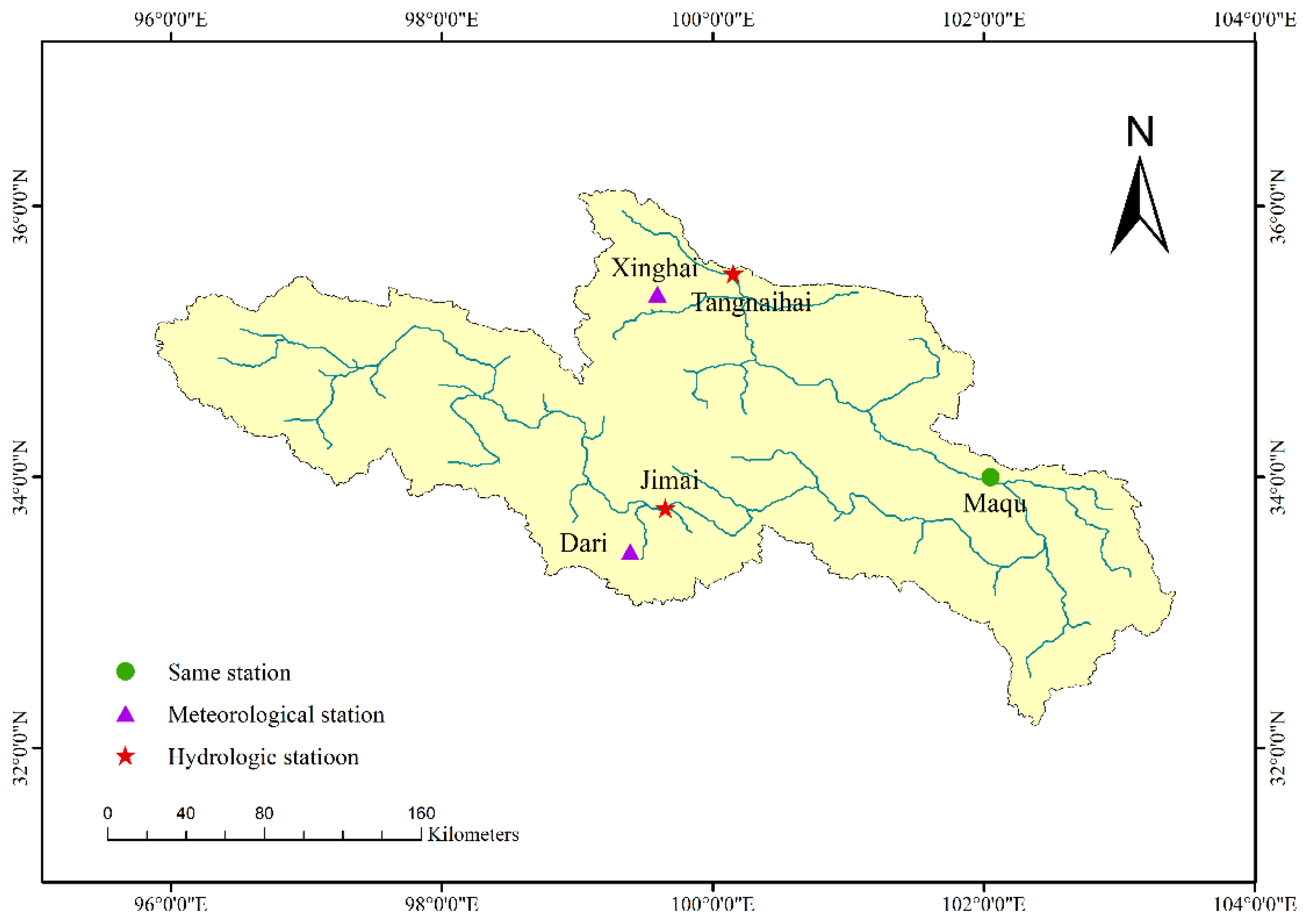
The source area of the Yellow River is located in the northeast of the Qinghai-Tibet Plateau. It refers to the basin above the Tangnaihai hydrological station, with a total area of about 132,000 km2, ranging from 95°50′ to 103°30′ E and 32°32′ to 36°10′ N. The source area of the Yellow River is a semi-humid area in the sub-cold zone of the Qinghai-Tibet Plateau, with an average elevation of 4217 m and an average annual temperature of −5.6 °C~3.8 °C. The precipitation is concentrated in July to September, and the distribution is extremely uneven. The average annual precipitation is 262.2–772.8 mm, and the annual average evaporation is 730–1700 mm [45].
There are many tributaries in the source area of the Yellow River, and precipitation is their main source. The average annual streamflow is 20.46 billion m3. It is the main water production area of the Yellow River basin. The source area of the Yellow River can generally be divided into three parts: the source-Jimai section, the Jimai-Maqu section, and the Maqu-Tangnaihai section. According to the characteristics of the river basin and the distribution characteristics of the stations in the source area, the monthly streamflow data of Jimai, Maqu, and Tangnaihai hydrological stations are used as the streamflow data. Precipitation and temperature data are collected from meteorological stations near the hydrological stations. As the Maqu hydrographic Station also has meteorological data, the meteorological stations in this study were Dari, Maqu, and Xinghai. Figure 1 shows the study area and the map of hydrologic and meteorological stations.
3.2. Data
The streamflow, precipitation, and temperature data in this study were obtained from the National Data Center for Meteorological Sciences (https://weather.cma.cn/ (accessed on 1 January 2019)) as shown in Table 1.
4. Results and Discussion
4.1. Model Input Variables Selection
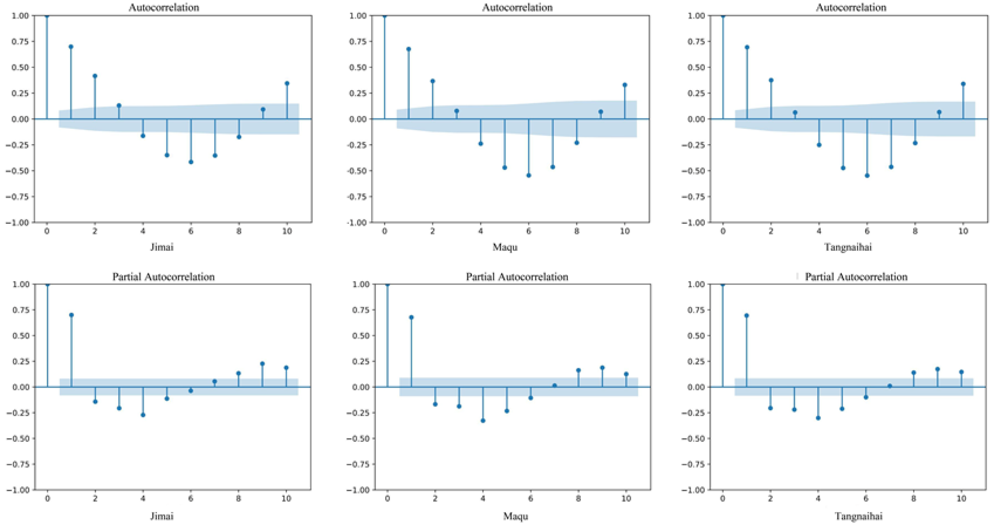
Firstly, the correlation between the current streamflow and the previous streamflow was calculated by ACF and PACF. The correlation of streamflow time series data was analyzed, and the input variables of streamflow were determined. Figure 2 shows the ACF and PACF results for the three stations, respectively. The streamflow lagged time of the three stations were roughly the same, and the lagged times of Jimai, Maqu, and Tangnaihai were 2 months. Then, TLCC was used to calculate the lagged time between precipitation and streamflow, temperature, and streamflow at the three stations. The lag order with the maximum Pearson correlation coefficient was selected as the lagged time, and the lagged time of precipitation and temperature of the three stations were all 1 month. In summary, the input variables for all three stations were , and the output variable was , where P represents rainfall, T represents temperature, Q represents runoff, and the subscript t represents the current time. In general, we can identify the ideal lag time and better comprehend and measure the impacts of various lag times on flow by categorizing temperature and precipitation with runoff and the lag time within runoff. This offers trustworthy hydrological data and decision assistance, and helps raise the accuracy of flow forecast models.
4.2. Model Structure Optimization
In the LSTM model, dropout and dense were set to 0.1 and 1, respectively. MSE is selected as the loss function, and grid search and cross-validation (GridSearchCV) were used to select the model optimizer and determine the optimal hyperparameters of the model, including the number of neurons, the number of epochs, and batch size. The number of neurons ranges from 1 to 401 with a step of 10, the number of epochs ranges from 1 to 500 with a step of 10, and the batch size ranges from 1 to 500 with a step of 10. Adam and Adadelta act as the optimizers. The optimal hyperparameters of the LSTM model of the three stations were determined according to the criterion of minimum loss function, as shown in Table 2.
4.3. Models Performance Comparison
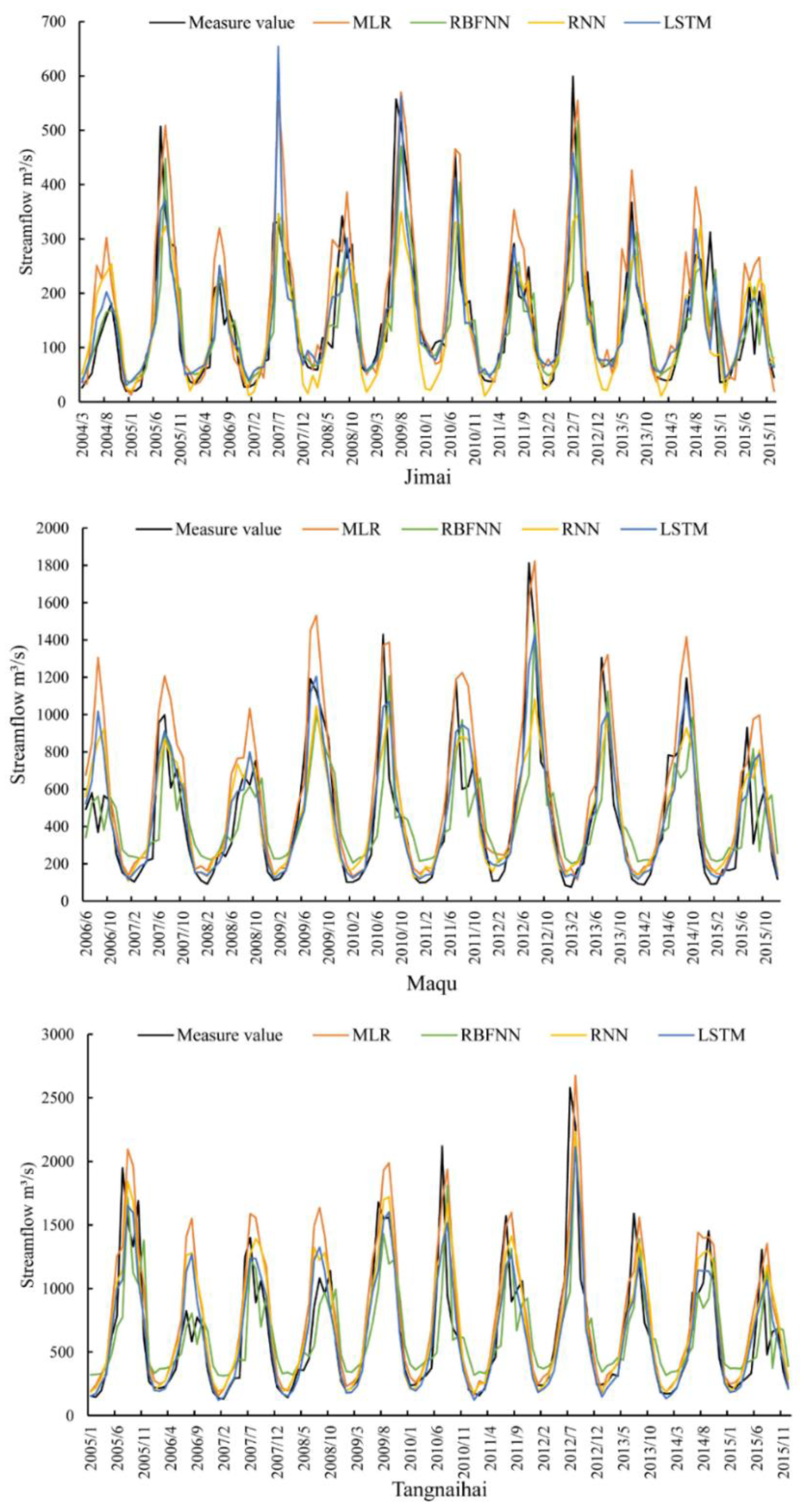
In this study, MLR, RBFNN, RNN, and LSTM models were used to compare the model performance of RMSE, R2, NSE, and KGE. Figure 3 shows the time series of the predicted streamflow values of the three stations in the study area. Table 3 shows the performance of four models at three stations during the calibration and validation period. From Figure 3 and Table 3, LSTM generally outperforms MLR, RBFNN, and RNN in terms of RMSE, MAE, R2, NSE, and KGE at the stations mentioned. At Jimai station, during calibration, LSTM outperforms MLR and RBFNN in terms of RMSE and MAE, and R2 is higher compared to MLR and RNN, both NSE and KGE are higher than other models. During validation, LSTM shows decreased RMSE and MAE and increased R2, NSE, and KGE compared to the other models. At Maqu station, during validation, the RMSE and MAE of the LSTM model were higher than MLR but lower than the other models, and R2, NSE, and KGE were significantly higher than all other models. At Tangnaihai station, during calibration, the performance of the metrics showed a similarity with those of Maqu station. The comparison shows that LSTM is particularly effective in different stations and periods, demonstrating its potential for accurate predictions in specific contexts.
The MLR model is considered to be less accurate than desired in the comparison of models discussed earlier, mainly due to its failure to account for nonlinear causation and variable interaction. While the MLR model assumes a linear connection between variables, the RBFNN model can identify complex nonlinear correlations between input and output data and can approximate any nonlinear function using the radial basis function as its activation function. However, RBFNN models are at risk of overfitting during the training phase, which can reduce their ability to predict new data. The RNN model, despite having a memory function, can analyze and forecast time series data and capture dynamic changes in the time dimension through loop connections. Nevertheless, the RNN model’s fully linked layer has higher memory requirements, is more difficult to train, and is more susceptible to gradient explosion and disappearance issues. The LSTM, a version of RNN, performs better in time series prediction by introducing a gating mechanism that effectively handles long-term reliance issues. The LSTM model has the best forecasting capacity for monthly flow prediction, followed by the RNN model, while the RBFNN model has a relatively weak forecasting ability. These conclusions are drawn from the characteristics of the mentioned models and the actual impacts of various stations.
4.4. Comprehensive Comparison of Different Models with or without Lagged Time
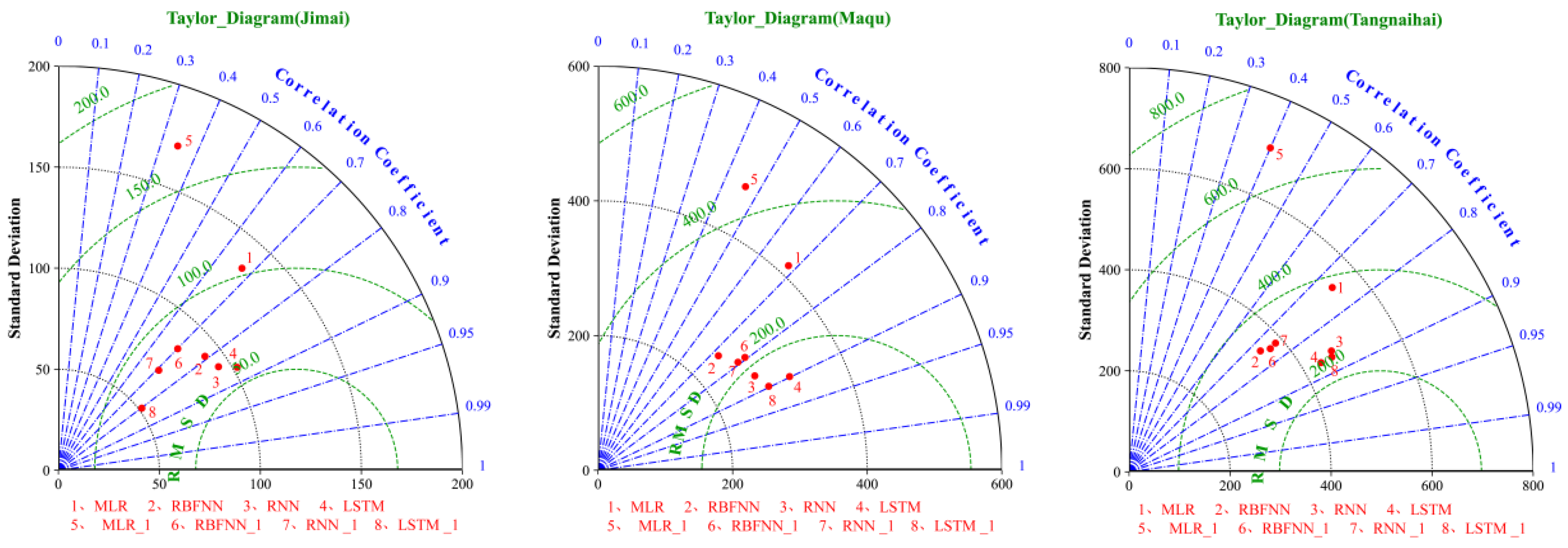
To further intuitively compare the monthly streamflow prediction ability of multiple models and the impact of lagged time on the models, this study selected Taylor diagram to reflect the advantages and disadvantages of the model in the monthly streamflow prediction under the influence of lagged time, and comprehensively evaluated the optimal statistical relationship combined with the metrics results. Figure 4 shows the Taylor diagram calculated from the time series of streamflow simulation values obtained by different models in the validation period with or without the influence of the lagged time. There were eight input and output models in total, including MLR, RBFNN, RNN and LSTM considering the lagged time, and MLR_1, RBFNN_1, RNN_1 and LSTM_1 without considering the lagged time. In Jimai station, MLR_1 has the largest standard deviation (SD), while LSTM has the smallest root mean square deviation (RMSD). LSTM also has the highest correlation coefficient (r) exceeding 0.85. In Maqu station, MLR_1 has the largest SD, while LSTM has the smallest RMSD and the highest correlation coefficient. In Tangnaihai station, MLR_1 has the largest SD, while LSTM has the smallest RMSD and the highest correlation coefficient. Overall, models considering lagged times have better predictive ability than those without lagged time. The LSTM model has the best predictive ability among the models considering lagged time.
5. Conclusions
In this study, the Long Short-Term Memory (LSTM) model was proposed for predicting monthly streamflow and tested at the Jimai, Maqu, and Tangnaihai stations in the source region of the Yellow River. The potential of Long Short-Term Memory (LSTM) in predicting monthly streamflow was explored and compared with the Multiple Linear Regression (MLR), Radial Basis Function Neural Network (RBFNN), and Recurrent Neural Network (RNN) models. The results indicated that grid search and cross-validation (GridSearchCV) can improve the efficiency of selecting model hyperparameters. The models incorporating ACF, PACF, and TLCC to account for lagged time were evidently superior to the models using the current variable as inputs. When accounting for the time delay, the LSTM model demonstrated superior predictive performance compared to the MLR, RBFNN, and RNN models at the three stations. The R2 improved by an average of 17.46%, 33.94%, and 15.29%, respectively. In this paper, a prediction framework was proposed that integrates the time lag of input variables. The LSTM model not only demonstrated good applicability in the source region of the Yellow River but also improved the prediction accuracy by considering the lag time of the impact factors. This provides a scientific method for water resource management in the source region of the Yellow River. In the future, we will endeavor to integrate LSTM with other methods to quantitatively analyze the key functions and input variables of the complex data-driven model. This will enable us to comprehend the fundamental decision-making process behind the model’s predictions and achieve interpretation of the complex data-driven model. Furthermore, through additional exploration and integration with the physical laws governing hydrological processes, the data-driven model can exhibit improved applicability. The LSTM model can also be expanded to encompass regions with diverse climate characteristics, thereby offering theoretical and technical support for streamflow prediction in various other regions.
Author Contributions
H.C. methodology, data curation, programming tune, writing—original draft; Z.W. writing—review and editing, methodology; C.N.: validation, data curation. All authors have read and agreed to the published version of the manuscript.
Funding
This work has been sponsored in part by the Major Science and Technology Projects of Qinghai Province (2021-SF-A6) and National Natural Science Foundation of China (42207070). Comments and suggestions from anonymous reviewers, the Associate Editor, and the Editor are greatly appreciated.
Data Availability Statement
Available from the corresponding author upon reasonable request.
Conflicts of Interest
The authors declare no conflict of interest.
References
- Wu, Q.H.; Ke, L.H.; Wang, J.D.; Pavelsky, T.M.; Allen, G.H.; Sheng, Y.W.; Duan, X.J.; Zhu, Y.Q.; Wu, J.; Wang, L.; et al. Satellites reveal hotspots of global river extent change. Nat Commun. 2023, 14, 1587. [Google Scholar] [CrossRef]
- Li, L.; Ni, J.; Chang, F.; Yue, Y.; Frolova, N.; Magritsky, D.; Borthwick, A.G.L.; Ciais Philippe Wang, Y.; Zheng, C.; Walling, D.E. Global trends in water and sediment fluxes of the world’s large rivers. Sci. Bull. 2020, 65, 62–69. [Google Scholar] [CrossRef] [PubMed]
- Hu, J.; Wu, Y.; Sun, P.; Zhao, F.; Sun, K.; Li, T.; Sivakumar, B.; Qiu, L.; Sun, Y.; Jin, Z. Predicting long-term hydrological change caused by climate shifting in the 21st century in the headwater area of the Yellow River Basin. Stoch. Environ. Res. Risk Assess. 2021, 36, 1651–1668. [Google Scholar] [CrossRef]
- Dalkilic, H.Y.; Hashimi, S.A. Prediction of daily streamflow using artificial neural networks (ANNs), wavelet neural networks (WNNs), and adaptive neuro-fuzzy inference system (ANFIS) models. Water Supply 2020, 20, 1396–1408. [Google Scholar] [CrossRef]
- Chu, H.B.; Wei, J.H.; Li, J.Y.; Qiao, Z.; Cao, J.W. Improved Medium- and Long-Term Runoff Forecasting Using a Multimodel Approach in the Yellow River Headwaters Region Based on Large-Scale and Local-Scale Climate Information. Water 2017, 9, 608. [Google Scholar] [CrossRef]
- Yang, J.J.; Wang, T.H.; Yang, D.W.; Yang, Y.T. Insights into runoff changes in the source region of Yellow River under frozen ground degradation. J. Hydrol. 2023, 617, 128892. [Google Scholar] [CrossRef]
- He, Z.B.; Wen, X.H.; Liu, H.; Du, J. A comparative study of artificial neural network, adaptive neuro fuzzy inference system and support vector machine for forecasting river flow in the semiarid mountain region. J. Hydrol. 2014, 509, 379–386. [Google Scholar] [CrossRef]
- Wang, Z.Y.; Qiu, J.; Li, F.F. Hybrid Models Combining EMD/EEMD and ARIMA for Long-Term Streamflow Forecasting. Water 2018, 10, 853. [Google Scholar] [CrossRef]
- Yin, H.L.; Zhang, X.W.; Wang, F.D.; Zhang, Y.N.; Xia, R.L.; Jin, J. Rainfall-runoff modeling using LSTM-based multi-state-vector sequence-to-sequence model. J. Hydrol. 2021, 598, 126378. [Google Scholar] [CrossRef]
- Nourani, V.; Komasi, M. A geomorphology-based ANFIS model for multi-station modeling of rainfall-runoff process. J. Hydrol. 2013, 490, 41–55. [Google Scholar] [CrossRef]
- Chu, H.B.; Wei, J.H.; Qiu, J. Monthly Streamflow Forecasting Using EEMD-Lasso-DBN Method Based on Multi-Scale Predictors Selection. Water 2018, 10, 1486. [Google Scholar] [CrossRef]
- Lian, Y.N.; Luo, J.G.; Xue, W.; Zuo, G.G.; Zhang, S.Y. Cause-driven Streamflow Forecasting Framework Based on Linear Correlation Reconstruction and Long Short-term Memory. Water Resour. Manag. 2022, 36, 1661–1678. [Google Scholar] [CrossRef]
- Londhe, S.; Charhate, S. Comparison of data-driven modelling techniques for river flow forecasting. Hydrol. Sci. J. 2010, 55, 1163–1174. [Google Scholar] [CrossRef]
- Yu, X.; Zhang, X.Q.; Qin, H. A data-driven model based on Fourier transform and support vector regression for monthly reservoir inflow forecasting. J. Hydro-Environ. Res. 2018, 18, 12–24. [Google Scholar] [CrossRef]
- Wu, Y.Q.; Wang, Q.H.; Li, G.; Li, J.D. Data-driven runoff forecasting for Minjiang River: A case study. Water Supply 2020, 20, 2284–2295. [Google Scholar] [CrossRef]
- Liu, Y.; Sang, Y.F.; Li, X.X.; Hu, J.; Liang, K. Long-Term Streamflow Forecasting Based on Relevance Vector Machine Model. Water 2017, 9, 9. [Google Scholar] [CrossRef]
- Lian, L. Runoff forecasting model based on CEEMD and combination model: A case study in the Manasi River, China. Water Supply 2022, 22, 3921–3940. [Google Scholar] [CrossRef]
- Modaresi, F.; Araghinejad, S.; Ebrahimi, K. A Comparative Assessment of Artificial Neural Network, Generalized Regression Neural Network, Least-Square Support Vector Regression, and K-Nearest Neighbor Regression for Monthly Streamflow Forecasting in Linear and Nonlinear Conditions. Water Resour. Manag. 2018, 32, 243–258. [Google Scholar] [CrossRef]
- Roy, B.; Singh, M.P.; Kaloop, M.R.; Kumar, D.; Hu, J.W.; Kumar, R.; Hwang, W.S. Data-Driven Approach for Rainfall-Runoff Modelling Using Equilibrium Optimizer Coupled Extreme Learning Machine and Deep Neural Network. Appl. Sci. 2021, 11, 6238. [Google Scholar] [CrossRef]
- Yang, S.Y.; Yang, D.W.; Chen, J.S.; Zhao, B.X. Real-time reservoir operation using recurrent neural networks and inflow forecast from a distributed hydrological model. J. Hydrol. 2019, 579, 124229. [Google Scholar] [CrossRef]
- Apaydin, H.; Feizi, H.; Sattari, M.T.; Colak, M.S.; Shamshirband, S.; Chau, K.W. Comparative Analysis of Recurrent Neural Network Architectures for Reservoir Inflow Forecasting. Water 2020, 12, 1500. [Google Scholar] [CrossRef]
- Zhu, S.; Luo, X.G.; Yuan, X.H.; Xu, Z.Y. An improved long short-term memory network for streamflow forecasting in the upper Yangtze River. Stoch. Env. Res. Risk. A. 2020, 34, 1313–1329. [Google Scholar] [CrossRef]
- Rahimzad, M.; Nia, A.M.; Zolfonoon, H.; Soltani, J.; Mehr, A.D.; Kwon, H.H. Performance Comparison of an LSTM-based Deep Learning Model versus Conventional Machine Learning Algorithms for Streamflow Forecasting. Water Resour. Manag. 2021, 35, 4167–4187. [Google Scholar] [CrossRef]
- Hu, C.H.; Wu, Q.; Li, H.; Jian, S.Q.; Li, N.; Lou, Z.Z. Deep Learning with a Long Short-Term Memory Networks Approach for Rainfall-Runoff Simulation. Water 2018, 10, 1543. [Google Scholar] [CrossRef]
- Kratzert, F.; Klotz, D.; Brenner, C.; Schulz, K.; Herrnegger, M. Rainfall-runoff modelling using Long Short-Term Memory (LSTM) networks. Hydrol. Earth Syst. Sci. 2018, 22, 6005–6022. [Google Scholar] [CrossRef]
- Ding, Y.K.; Zhu, Y.L.; Feng, J.; Zhang, P.C.; Cheng, Z.R. Interpretable spatio-temporal attention LSTM model for flood forecasting. Neurocomputing 2020, 403, 348–359. [Google Scholar] [CrossRef]
- Song, T.Y.; Ding, W.; Wu, J.; Liu, H.X.; Zhou, H.C.; Chu, J.G. Flash Flood Forecasting Based on Long Short-Term Memory Networks. Water 2020, 12, 109. [Google Scholar] [CrossRef]
- Bakhshi Ostadkalayeh, F.; Moradi, S.; Asadi, A.; Moghaddam Nia, A.; Taheri, S. Performance improvement of LSTM-based deep learning model for streamflow forecasting using Kalman filtering. Water Resour. Manag. 2023, 37, 3111–3127. [Google Scholar] [CrossRef]
- Hunt, K.M.; Matthews, G.R.; Pappenberger, F.; Prudhomme, C. Using a long short-term memory (LSTM) neural network to boost river streamflow forecasts over the western United States. Hydrol. Earth Syst. Sci. 2022, 26, 5449–5472. [Google Scholar] [CrossRef]
- Nourani, V.; Partoviyan, A. Hybrid denoising-jittering data pre-processing approach to enhance multi-step-ahead rainfall-runoff modeling. Stochastic Stoch. Env. Res. Risk. A. 2018, 32, 545–562. [Google Scholar] [CrossRef]
- Hameed, M.M.; Alomar, M.K.; Al-Saadi, A.A.A.; Alsaadi, M.A. Inflow forecasting using regularized extreme learning machine: Haditha reservoir chosen as case study. Stoch. Env. Res. Risk. A. 2022, 36, 4201–4221. [Google Scholar] [CrossRef]
- Tran, T.D.; Kim, J. Machine learning modeling structures and framework for short-term forecasting and long-term projection of Streamflow. Stoch Environ. Res. Risk Assess. 2023. [Google Scholar] [CrossRef]
- Liu, M.Y.; Huang, Y.C.; Li, Z.J.; Tong, B.X.; Liu, Z.T.; Sun, M.K.; Jiang, F.Q.; Zhang, H.C. The Applicability of LSTM-KNN Model for Real-Time Flood Forecasting in Different Climate Zones in China. Water 2020, 12, 440. [Google Scholar] [CrossRef]
- Vu, M.T.; Jardani, A.; Massei, N.; Fournier, M. Reconstruction of missing groundwater level data by using Long Short-Term Memory (LSTM) deep neural network. J. Hydrol. 2021, 597, 125776. [Google Scholar] [CrossRef]
- Gao, S.; Huang, Y.F.; Zhang, S.; Han, J.C.; Wang, G.Q.; Zhang, M.X.; Lin, Q.S. Short-term runoff prediction with GRU and LSTM networks without requiring time step optimization during sample generation. J. Hydrol. 2020, 589, 125188. [Google Scholar] [CrossRef]
- Alizadeh, B.; Bafti, A.G.; Kamangir, H.; Zhang, Y.; Wright, D.B.; Franz, K.J. A novel attention-based LSTM cell post-processor coupled with Bayesian optimization for streamflow prediction. J. Hydrol. 2021, 601, 126526. [Google Scholar] [CrossRef]
- Bai, P.; Liu, X.M.; Xie, J.X. Simulating runoff under changing climatic conditions: A comparison of the long short-term memory network with two conceptual hydrologic models. J. Hydrol. 2021, 592, 125779. [Google Scholar] [CrossRef]
- Wang, Z.Q.; Si, Y.; Chu, H.B. Daily streamflow prediction and uncertainty using a long short-term memory (LSTM) network coupled with bootstrap. Water Resour. Manag. 2022, 36, 4575–4590. [Google Scholar] [CrossRef]
- Rumelhart, D.E.; Hinton, G.E.; Williams, R.J. Learning representations by back propagating errors. Nature 1986, 323, 533–536. [Google Scholar] [CrossRef]
- Chu, H.B.; Wu, J.; Wu, W.Y.; Wei, J.H. A dynamic classification-based long short-term memory network model for daily streamflow forecasting in different climate regions. Ecol Indic. 2023, 148, 110092. [Google Scholar] [CrossRef]
- Kratzert, F.; Klotz, D.; Shalev, G.; Klambauer, G.; Hochreiter, S.; Nearing, G. Towards learning universal, regional, and local hydrological behaviors via machine learning applied to large-sample datasets. Hydrol. Earth Syst. Sci. 2019, 23, 5089–5110. [Google Scholar] [CrossRef]
- Wang, L.F.; Xu, B.; Zhang, C.; Fu, G.T.; Chen, X.X.; Zheng, Y.; Zhang, J.J. Surface water temperature prediction in large-deep reservoirs using a long short-term memory model Surface water temperature prediction in large-deep reservoirs using a long short-term memory model. Ecol Indic. 2022, 134, 108491. [Google Scholar] [CrossRef]
- Parmar, K.S.; Bhardwaj, R. Statistical, time series, and fractal analysis of full stretch of river Yamuna (India) for water quality management. Environ. Sci. And Pollut. Res. 2015, 22, 397–414. [Google Scholar] [CrossRef] [PubMed]
- Zhang, X.; Chen, B.B.; Gong, H.L.; Lei, K.C.; Zhou, C.F.; Lu, Z.Z.; Zhao, D.N. Inversion of Groundwater Storage Variations Considering Lag Effect in Beijing Plain, from RadarSat-2 with SBAS-InSAR Technology. Remote Sens. 2022, 14, 991. [Google Scholar] [CrossRef]
- Li, Z.J.; Li, Z.X.; Qi, F.; LiU, X.Y.; Gui, J.; Xue, J. Quantitative analysis of recharge sources of different runoff types in the source region of Three River. J. Hydrol. 2023, 626, 130366. [Google Scholar] [CrossRef]
Figure 1.
The study area and the map of hydrological and meteorological stations.

Figure 2.
ACF and PACF plots of Jimai, Maqu and Tangnaihai.

Figure 3.
Time series of MLR, RBFNN, RNN, and LSTM predicted results at different stations.

Figure 4.
Taylor diagram obtained by the time series of the simulated values of the eight models in the validation period of the three stations.
Figure 4.
Taylor diagram obtained by the time series of the simulated values of the eight models in the validation period of the three stations.


Table 1.
The stations used for the calibration and validation in this study.
| Station | Longitude | Latitude | Time Span | Average Annual Temperature | Average Annual Precipitation | Average Annual Streamflow |
|---|---|---|---|---|---|---|
| Dari | 33.45 | 99.39 | 1956–2015 | −0.785 | 153.986 | |
| Xinghai | 35.35 | 99.56 | 1960–2015 | 1.438 | 102.495 | |
| Maqu | 34.00 | 102.05 | 1967–2015 | 1.718 | 168.923 | 452.087 |
| Jimai | 33.76 | 99.65 | 1956–2015 | 127.698 | ||
| Tangnaihai | 35.5 | 100.15 | 1960–2015 | 648.235 |
Table 2.
Optimal hyperparameters Settings of LSTM model at three stations.
| Station | Dropout | Dense | Neuron | Epoch | Batch Size | Optimizer |
|---|---|---|---|---|---|---|
| Jimai | 0.1 | 1 | 311 | 301 | 101 | Adam |
| Maqu | 0.1 | 1 | 91 | 101 | 101 | Adam |
| Tangnaihai | 0.1 | 1 | 101 | 201 | 11 | Adam |
Table 3.
Performance of MLR, RBFNN, RNN and LSTM during calibration and validation periods at different stations.
Table 3.
Performance of MLR, RBFNN, RNN and LSTM during calibration and validation periods at different stations.
| Model | Calibration | Validation | |||||||
|---|---|---|---|---|---|---|---|---|---|
| MLR | RBFNN | RNN | LSTM | MLR | RBFNN | RNN | LSTM | ||
| Jimai | R2 | 0.57 | 0.60 | 0.66 | 0.74 | 0.63 | 0.61 | 0.69 | 0.77 |
| RMSE | 57.12 | 73.10 | 67.18 | 60.14 | 60.39 | 72.92 | 65.22 | 56.53 | |
| MAE | 37.02 | 44.97 | 46.06 | 42.94 | 41.80 | 45.33 | 43.60 | 40.54 | |
| NSE | 0.55 | 0.58 | 0.66 | 0.71 | 0.59 | 0.62 | 0.69 | 0.75 | |
| KGE | 0.57 | 0.64 | 0.68 | 0.77 | 0.65 | 0.77 | 0.72 | 0.82 | |
| Maqu | R2 | 0.53 | 0.49 | 0.67 | 0.73 | 0.60 | 0.52 | 0.73 | 0.81 |
| RMSE | 196.58 | 270.50 | 217.58 | 196.06 | 154.74 | 244.20 | 185.54 | 155.93 | |
| MAE | 116.97 | 184.99 | 132.31 | 118.40 | 98.86 | 176.85 | 118.41 | 100.23 | |
| NSE | 0.62 | 0.66 | 0.81 | 0.85 | 0.70 | 0.72 | 0.84 | 0.89 | |
| KGE | 0.50 | 0.56 | 0.68 | 0.75 | 0.56 | 0.59 | 0.71 | 0.83 | |
| Tangnaihai | R2 | 0.47 | 0.51 | 0.70 | 0.69 | 0.52 | 0.54 | 0.71 | 0.75 |
| RMSE | 287.87 | 363.60 | 283.60 | 285.87 | 249.77 | 337.39 | 266.36 | 247.20 | |
| MAE | 171.77 | 249.59 | 179.44 | 164.60 | 149.91 | 238.95 | 174.47 | 146.43 | |
| NSE | 0.60 | 0.73 | 0.77 | 0.80 | 0.68 | 0.77 | 0.86 | 0.88 | |
| KGE | 0.54 | 0.60 | 0.75 | 0.80 | 0.62 | 0.61 | 0.77 | 0.83 | |
Disclaimer/Publisher’s Note: The statements, opinions and data contained in all publications are solely those of the individual author(s) and contributor(s) and not of MDPI and/or the editor(s). MDPI and/or the editor(s) disclaim responsibility for any injury to people or property resulting from any ideas, methods, instructions or products referred to in the content. |
© 2024 by the authors. Licensee MDPI, Basel, Switzerland. This article is an open access article distributed under the terms and conditions of the Creative Commons Attribution (CC BY) license (https://creativecommons.org/licenses/by/4.0/).
Share and Cite
MDPI and ACS Style
Chu, H.; Wang, Z.; Nie, C. Monthly Streamflow Prediction of the Source Region of the Yellow River Based on Long Short-Term Memory Considering Different Lagged Months. Water 2024, 16, 593. https://doi.org/10.3390/w16040593
AMA Style
Chu H, Wang Z, Nie C. Monthly Streamflow Prediction of the Source Region of the Yellow River Based on Long Short-Term Memory Considering Different Lagged Months. Water. 2024; 16(4):593. https://doi.org/10.3390/w16040593
Chicago/Turabian StyleChu, Haibo, Zhuoqi Wang, and Chong Nie. 2024. "Monthly Streamflow Prediction of the Source Region of the Yellow River Based on Long Short-Term Memory Considering Different Lagged Months" Water 16, no. 4: 593. https://doi.org/10.3390/w16040593
Note that from the first issue of 2016, this journal uses article numbers instead of page numbers. See further details here.