
Do Irrigation Water Requirements Affect Crops’ Economic Values?

1
Department of Economics, Roma Tre University, 00145 Rome, Italy
2
Consorzio di Bonifica per il Canale Emiliano Romagnolo, 40137 Bologna, Italy
*
Author to whom correspondence should be addressed.
Water 2024, 16(1), 77; https://doi.org/10.3390/w16010077
Submission received: 20 October 2023
/
Revised: 15 December 2023
/
Accepted: 20 December 2023
/
Published: 24 December 2023
(This article belongs to the Special Issue Economics of Water Management)
Abstract
:The irrigation water requirements of different crops are becoming a pivotal driver for the governance strategies of water allocation and management. This paper estimates the impact of irrigation water requirements on economic value in terms of the yields and gross saleable production of 13 different crops cultivated in the Emilia-Romagna region (Italy) over the 2010–2020 period by exploiting a generalized propensity score matching approach. Results show that the overall irrigation water requirements affect crops’ economic value. There is a causal effect of water irrigation on economic value: positive only for high levels of water irrigation in the case of yields, while it reverses and assumes a concave shape for gross saleable production. However, the effect is mediated by the irrigation water requirements of different crops. In water scarcity conditions, the allocation of water to arboreal crops, given the effect of water irrigation on gross saleable production, is also positive for small quantities of water. This paper can help guide the design of more sustainable water management strategies and agricultural development policies to face climate change.
1. Introduction
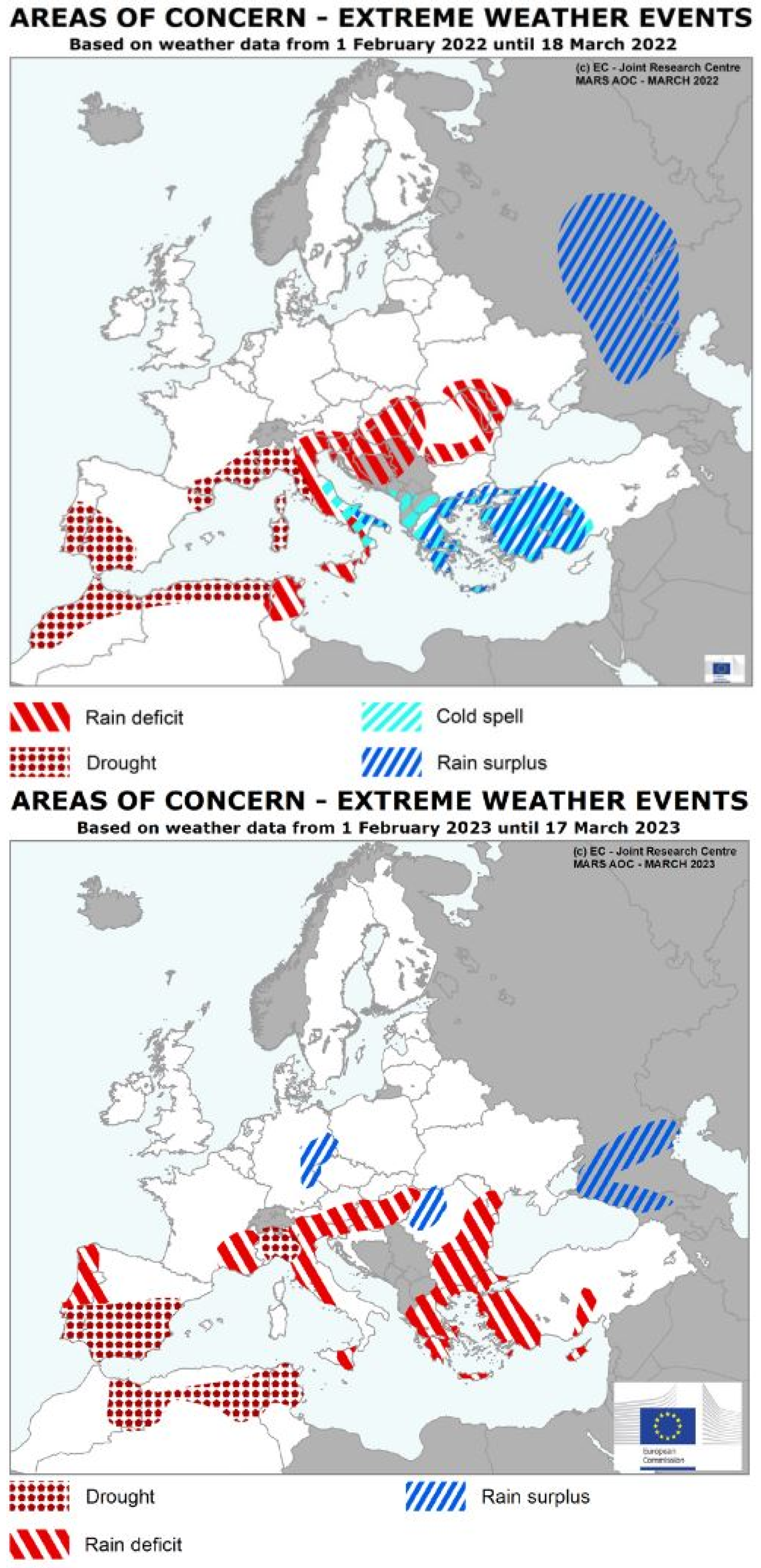
Climate change affects the agriculture and agri-food sector from different perspectives and through different channels. Among them, a special role is played by water scarcity. Indeed, the deep changes across the overall water cycle have brought about unconventional, and extreme, drought and flood events which represent major climate stressors for crop production [1]. These events affect the agriculture and agri-food sector, both in the short and in the long term. For instance, while on the one hand, crops could be damaged by floods, on the other, a drought extended over time can affect soil quality and its essential role within the ecosystem. At the same time, crops are stressed by increasing temperatures, as the ones experienced during 2022 and 2023, where rain deficits accumulated in the last part of winter (Figure 1 for the EU scenario) went along with high temperatures in the subsequent summer.
Agriculture is a water intensive sector, and actors (mainly farmers) are constantly facing irrigation criticalities.
According to the Water Exploitation Index provided by the European Environmental Agency, most EU countries account for water stress conditions, especially in the Mediterranean basin [4]. Italy is no exception and indeed it displays the 5th highest value of the Water Exploitation Index + [5] among European Union countries in 2019. The Water Exploitation Index + correlates water consumption as a fraction of renewable freshwater resources. Generally, values below 20% are considered to be good while values above 40% testify to severe water stress. In 2019, Italy’s value was 57%. It is worth mentioning that this ranking also remarks the stronger tie between irrigation and agriculture displayed by countries in Southern Europe, whose water resources are thus inevitably more stressed [6].
According to the JRC Bulletin [7,8], some Italian regions, such as the Po valley, faced the driest and hottest years ever recorded in 2022 and 2023. In this context, irrigation is enriched by a mitigation strategy dimension to deal with climate change since (i) it protects crops from climate variability and (ii) reduces crop temperatures, especially during heatwaves [9,10]. However, the availability of water irrigation is itself linked to climate dynamics. In particular, global warming and extreme events can affect crop production through many channels, such as the increasing demand for water from farmers and producers, and the volume and geographical diffusion of water bodies suitable for irrigation [11].
According to the existing literature, irrigation water requirements assume a key value for the agricultural, and agri-food sector, not only for agronomic reasons (i.e., the need for water as an input), but also for the economic value that in the actual climate scenario has been reached [12]. From the economic perspective, in fact, the economic value of water irrigation is mainly shaped by supply scarcity, which converts water in the nature of both an excludable club good (shared irrigation) as well as a rival common-pool good (natural water basins). The management of water irrigation therefore becomes a complex issue that countries and regional authorities organize in different ways.
In Italy, water issues are a regional policy concern, as established by the 2005 Constitutional Reform. Within each region, but with variable forms, there are reclamation and irrigation consortia, which are public law subjects that deal with the maintenance of land reclamation infrastructures and agriculture [13,14].Within the specific Italian framework, it is not mandatory to be part of a consortium, nor it is compulsory to buy the irrigation services of one of them. Still, everyone which falls under the consortium administrative area has to pay a fee since many of its activities in the field benefit heterogeneous subjects (farmers, factories and citizens). Consortia set a collective irrigation network which, under a regional policy point of view, allows for better water management. For example, the entire administrative area of Emilia-Romagna is covered by the operations of many different consortia, thus giving researchers the possibility to carry out analyses on a higher level. According to the National board of consortia, slightly more than half the national territory (59.47%) is covered.
In this context, the contribution of this paper is to investigate, for the first time in the literature, the effect of irrigation water requirements on the economic value at the territorial level by using quasi-experimental techniques for causal estimations, looking at the entire agricultural sector of an entire region, and considering different outcome of economic value. More specifically, the aim of the paper is to address the following research questions:
RQ1: Do irrigation water requirements affect crops’ economic values?
RQ2: If yes, to what extent does the impact of water irrigation on economic value depend on water endowment?
RQ3: Does the impact change across crop production?
Building on the most recent existing literature [15], we answer these questions by looking at the production of 13 crops in one of the EU’s Mediterranean regions where the agricultural sector is most relevant and that has been one of the most stressed by water crisis (Emilia-Romagna, Italy) and conducting the analysis at the NUTS3-crop level over the 2010–2020 period (Table A1). The crops included in the sample are: Actinidia, alfalfa, corn, grape, green bean, melon, onion, peach, pear, potato, soy, sugar beet and tomato (processing).
We use data from the Italian Farm Account Data Network European database (i.e., RICA), complemented by official territorial statistics (source: EUROSTAT) and agrometeorological data (source: ISTAT).
Methodologically, the analysis exploits generalized propensity score matching (GPS) methods for continuous treatment where the treatment is the irrigation water requirements (in the rest of the paper we refer to irrigation water requirements as IWR) [16]. As far as the economic outcome variables are concerned, we use yields and gross saleable production. The gross saleable production includes the revenues strictly connected with the agricultural activity.
This paper contributes to the strand of the literature about natural resource management and sustainable agricultural production in several ways. First of all, to the best of our knowledge, it is the first contribution that empirically estimates the relation between water requirements and economic value and presents results that can be useful to design sustainable development policies.
Secondly, our analysis provides results also at the crop level for different crops, rather than for only the production of one crop or at an aggregate level (agriculture). Given the heterogeneity across crops, and their agronomic requirements, it is particularly relevant to conduct the analysis separately across crops. In fact, the findings can provide insights for policy makers and practitioners to manage crop transition across territories in response to the predicted climate change. In this paper we look at one specific agriculture system, but the analysis can be easily replicated for other regions or at the national level to better inform policy makers and institutions.
2. Materials and Methods
2.1. Literature
Several studies exist that investigate the economic value of irrigation. Negri et al. [17] study the impact of climate change events in the U.S, especially in temperature and precipitation, on the decision to adopt irrigation by looking only at the production perspective. They adopt a micro-founded multi output production model to simulate different climatic scenarios and provide estimates of what would be happened with different farmer’s choices: irrigation is indeed adopted as a response to variations in the tails of temperature and precipitation distribution, but they are not the only explanatory variables as farm size and soil condition have a role as well.
Da Cunha et al. [18] carry on a two-stage study in the Brazilian scenario by considering (i) how climate influences irrigation adoption and (ii) how farmer adaptation to climate affects land values. They highlight that socioeconomic and agronomic variables as well as climatic ones are important in the decision process. Indeed, they show that, ceteris paribus, small farms tend to irrigate less than big commercial ones, due to the highly heterogeneous and relevant costs of irrigation, which are not so easy to manage for small farms.
By using the World Bank dataset for South America, Seo [19] investigates whether public adaptation to climate change is different from the private one. The focus is on irrigation and its dual nature, i.e., private or public schemes and finds that public schemes are characterized by their lump-sum nature thus conducting either to too much or too little water supply.
At the same time, a different strand of literature focuses on the offsetting effect of irrigation against climate change. Among others, Tack et al. [20] look at the mitigating effect of irrigation on wheat crops in severe high temperature conditions and they find that irrigation could offset the estimated negative impact on wheat yields (−8%) of every one-degree Celsius increase in temperature. Zaveri and Lobell [21] focus on India over the 1970–2009-period and conclude that irrigation allowed the achievement of higher wheat yields. By the construction of a counterfactually inspired scenario, they confront the observed output, i.e., the one with irrigation and the unobserved one, i.e., the one identified by irrigation levels and weather of 1970, supposing they were steady throughout time. In Li and Troy [22], a central part is dedicated to the impact of specific climatic variables on the difference between irrigated and rainfed crop yields and concludes that irrigation’s impact on it us variable but positive, and that for some crops (wheat), it is better not to irrigate as the impact on water resources is stronger than the benefit from irrigation.
Finally, the role of irrigation in agriculture is assessed in [15]: the authors stress that irrigation water has a relevant role in agriculture, but it seems not more important, less relevant even, than the type of farming and variable costs borne by the farm.
Methodologically, the existing literature has mainly adopted three approaches, which have, however, some criticalities and do not allow for the estimation of the causal impact. First, some papers investigate water irrigation issues by adopting the so-called residual value method, as described by Young and Loomis [23]: the value of production is decomposed by the value of each one of its inputs minus one, i.e., irrigation water, thus attributing to the latter the full residual value. While the main advantage of this approach is that it is straightforward and provides easily read results, the main disadvantage is that, accepting the neoclassical framework, it also attributes all kinds of things that affect the production function but that were not possible to detect to water value.
A different group of studies relies on the stated preferences approach [24]. The value of the water irrigation is accounted here starting from what the sample of people interviewed declare, i.e., their willingness to pay. This methodology has some limitations: (i) the necessity of a well-selected sample, (ii) the construction of a structured survey; and (iii) the nature of the analysis are a few of the main weaknesses of this approach. However, they have been demonstrated to be quite useful when speaking of non-market benefits. Lastly, some of the existing papers exploit the hedonic price approach [11,25]. However, the assumption of perfect market competition, and thus that land prices are a perfect function of its attributes is critical for the reliability of the analysis.
2.2. Data
To conduct the analysis, we rely on a dataset that we arrange from different sources of data and that include a set of climatic, agronomic and socioeconomic variables at the NUTS3-crop-year level over the 2010–2020 period.
Climatic data come from the Italian Agenzia regionale per la prevenzione, l’ambiente e l’energia dell’Emilia-Romagna (Arpae) that provides daily records from 1961 to 2020 about precipitation and minimum and maximum temperatures [26] (Available at https://dati.arpae.it/dataset/erg5-eraclito. Last access on 1 April 2023). Starting with them, we calculated the following agroclimatic indicators. First, we calculated the 90th percentile of the entire time series at NUTS3 level for minimum and maximum temperature (IS_TNover90p and IS_TXover90p). We quantified the total amount of days with temperature above the 90th percentile and defined a heatwave when there were at least three consecutive days over the 90th percentile and the heatwave number (TN_HWN and TX_HWN) as the total of the heatwaves across one year [27].As stated in [27], it is possible to apply the abovementioned heatwave definition either in terms of maximum temperature (TX) or minimum temperature (TN). For precipitation, we considered the days with effective rainfall as the days with precipitation above 2.5 mm (0.1 inch) and the days with heavy rainfall as the ones characterized by precipitation above 25 mm (1 inch) [17] (IS_rainydays and IS_Heavyrainydays, respectively).We are aware of the many existing linkages between the paucity of precipitation in winter and drought problems in the subsequent summer, but we will not address this topic in this work. We will focus mainly on what happens during the irrigation season (IS), which usually goes from April to October. However, the evidence arising from the data drove us to define it as the time span that goes from the first decade of March to the last decade of November.
Water and agronomic data were gathered from Consorzio di Bonifica per il Canale Emiliano Romagnolo (CER), which is a second level consortium whose activities pertain to an important part of the region and consist in information on the irrigated dimension of acreage and yields for the area of interest.
In particular, we collected IWR by the means of Irriframe [28], a digital platform developed by CER whose utility to support better water management practices in Europe has already been proved [29].
Data on gross saleable production and the characteristics of the local agricultural sector come from the Italian Farm Accountancy Data Network database, i.e., RICA (FADN, 2022).The FADN is the most important source of annual micro-economic data for agricultural holdings within EU. One of its greatest advantages lies in the harmonized and standardized practice of its construction, which makes comparisons between countries possible. The Italian sample is made up of 10,764 farms. In extracting data from FADN, we used the following criterion: we considered every fully irrigated crop as irrigated, i.e., when the entire acreage dedicated to that particular crop was irrigated (see https://rica.crea.gov.it/ for more information, last access on 1 April 2023). Lastly, data from ISTAT was used to cover possible observation gaps in the acreage and yields item, while data on per capita GDP come from EUROSTAT.See Table 1 for source and descriptive statistics of the variables we used while Table A2 for their definition.
2.3. Research Scenario
The final sample is an unbalanced panel of 8 NUTS3 areas of the Emilia-Romagna region and 13 different crops followed from 2010 to 2020 for a total of 609 observations. The sample does not include the NUTS3 Rimini due to its inadequate data coverage.
Emilia-Romagna is one of the most productive regions in Italy for the agricultural and agri-food sector. It accounted for approximately 9.16% of the national gross domestic product in 2021 and for the 11.8% of the value of the national agricultural output in 2020). Its geographical position allows for the existence of a high-quality and highly heterogenous food industry, as proven by the 44 European protected denomination items. According to 7th Agricultural Census data mentioned by Emilia-Romagna Region, within Emilia-Romagna the utilized agricultural area (UAA) is equals to 1045 thousands of hectares, about the 79% of the total agricultural area, in slightly decrease of 1.8% and 2.6%, respectively from 2010.
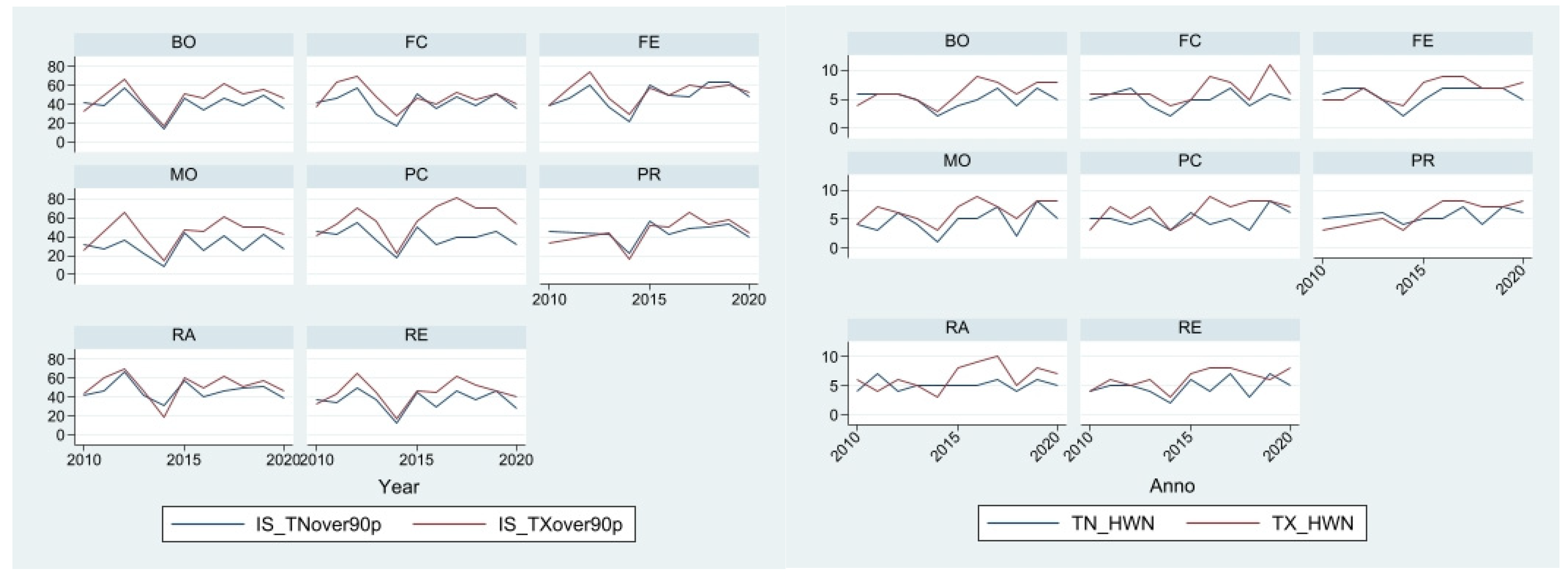
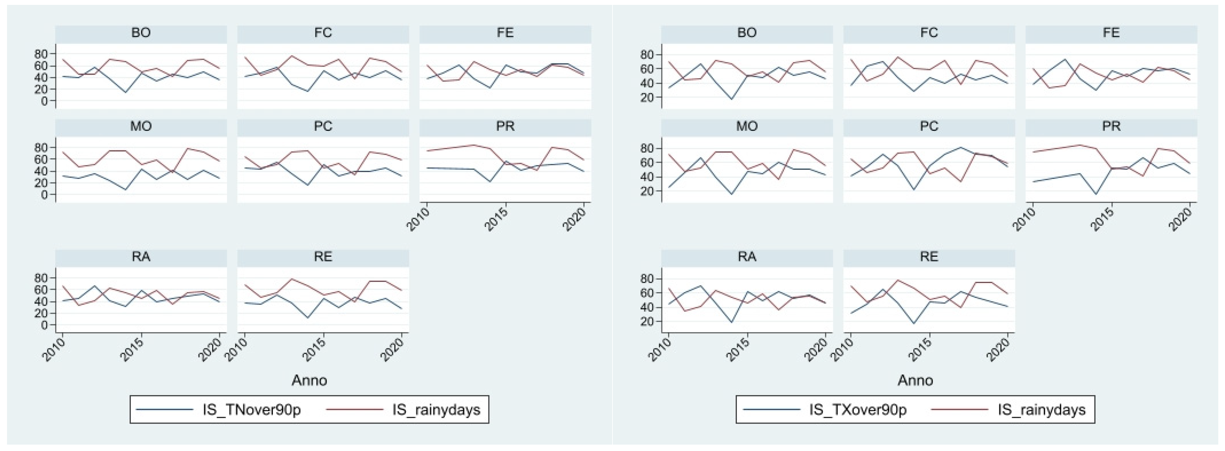
The region has a milder climate compared to other Italian regions. Still, it has not been immune to climate change. Figure 2 depicts anomalies only considering maximum and minimum temperature: to this definition, it seems quite clear that 2014 has been the coolest year of our time span of interest. Instead, to look at the hottest ones, we would have to at least simultaneously consider both temperature and precipitation: as described by Figure 3, the 2012–2013 pair as well as 2017 emerge.
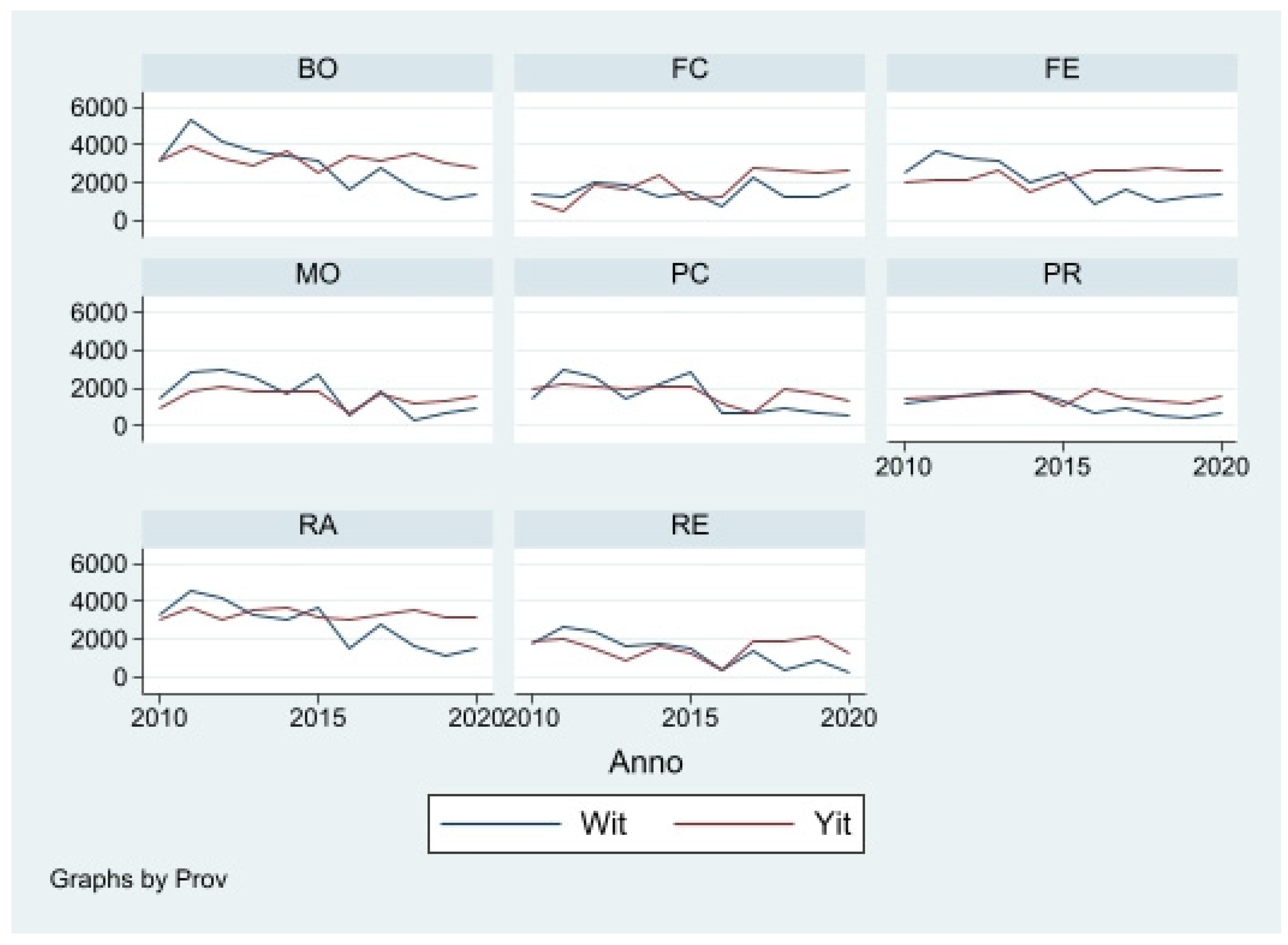
Finally, we do not have data regarding the full stock of water available for irrigation within every NUTS3 area. Instead, we have data on crop water requirements, defined as IWRthat for its inherent characteristics we can consider as the crops’ minimum demand for water or, roughly speaking, the inferior threshold of irrigation water. Given that the IS generally goes from the first decade of March to the final decade of November, IWR is calculated as the average water demand by crop j not over the entire IS, but only over the exact period of its irrigation. We plotted the unitary heterogenous IWR across crops and for time t at the NUTS3 level (Wit) and did the same for yields (Yit) in Figure 4.
On average, a decrease in demanded water emerges, with a particularly falling movement for Bologna, Ferrara, Ravenna and Reggio Emilia. The same trend does not hold for yields which do not follow a decreasing path, but rather a more irregular one. According to the Emilia-Romagna Region (2021), the 2020/2010 delta of the yields for the crops considered within our analysis was a decrease of 18% (see https://statistica.regione.emilia-romagna.it/agricoltura/produzione-lorda-vendibile-a-prezzi-correnti, last access on 19 October 2023). It is interesting to note that three out of the four abovementioned areas are in the eastern part of the region, which lacks abundant water resources and is strongly dependent on CER services.
2.4. Methodology
According to Negri et al. [17], the farmer’s decision-making process can be defined as follows:
where I and D indicates irrigated and dryland, respectively; Y(.) are the production possibilities set by constraints on technology, land (N), land quality (, i.e., soil and climate and irrigation capacity (T); P and W are the exogenous output and input prices; Y and X are agricultural output and input, respectively; T represents the discrete choice whether to adopt irrigation or not and is the irrigation cost.
Aimed at the achievement of the optimum possible profit level, each farmer will decide whether to adopt irrigation. However, in our analysis, IWR is not directly linked to profit, rather it is linked to gross saleable production generating endogeneity and self-selection issues. To solve it, we rely on generalized propensity score matching (GPS) for continuous treatment [16]. The GPS extends the binary treatment proposed by Rosenbaum and Rubin [30] to continuous treatment scenarios with the aim of balancing the distribution of covariates in the treated and control group [31]. Several papers recently used this approach to evaluate agrifood policies, including [32,33]. In this paper, in fact, all NUTS3 crop observations are treated (irrigated), but with different levels of treatment. Thanks to the GPS we are, therefore, capable of estimating how the impact changes for different levels of treatment intensity.
From the empirical perspective, the GPS first assigns a score in terms of treatment probability and second, it compares observations with the most similar score in order to isolate the performance ascribable to the treatment. Then, it estimates the causal impact of a unitary change in the treatment level by using the dose–response function approach. The model produces two outcomes: the dose–response function (DRF) and the treatment effect function (TEF).
In this paper, we considered IWR as the treatment and looked at the yields and gross saleable production as proxies of economic values. Due to the absence of data on the exact amount of supplied water, IWR can be considered a good proxy of the latter given that irrigation water gravitates around IWR and is surely correlated with it. Operationally, the GPS model, as illustrated in Hirano and Imbens [16] and Imbens [34] relies on the assumption of weak confoundedness. If we define as the potential outcome of the individual i when exposed to the treatment t, then we can formulate it as follows:
It means that, given the covariates X for each individual, the potential outcome is orthogonal with respect to the treatment assignment. This assumption derives directly from Rosenbaum and Rubin [30] and in its original form, it involves the unbiasedness of the difference between the treatment and control means as the average treatment effect. In the GPS case, it is not necessary for this to hold, and indeed the weak unconfoundedness only requires the conditional independence of each value of the treatment, not the joint one [16].
One of the main utilities of GPS allows us to observe not only the average irrigation effect on yields (, but also the marginal one (),
In other words, we need to construct a function that allows us to operate the best comparison among our units. This function is the propensity score and is a function of the covariates of each unit. More precisely, it is the conditional probability of receiving the treatment, given the covariates:
which, in turn, leads us to the define the GPS as . Another trait of the methodology is the balancing property, namely:
where I(.) is the indicator function. Equation (5) states that within layers marked by the same value of the propensity score, the probability that T = t is not dependent upon the value of X.
At this point, the practical implementation of the GPS is divided into three parts [35].
The first requires the estimation of the propensity score . Treatment is assumed to be normally distributed, conditional on covariates. Since our treatment does not follow this path, we use an ln transformation and then tested its normality by the skewness and kurtosis test:
where is the transformation of our treatment and is function of covariates with linear and high order terms, dependent on a vector of parameters. To complete the first step, we estimate the GPS as [35]:
where and are estimated from Equation (6). If Equation (5) holds, we can consider observations within the same layer to be identical among them, orthogonally with respect to the actual treatment level. The second part of the procedure deals with the conditional expectation of the outcome given the treatment ( and GPS ( [35]. We estimate the following:
with being a vector of parameter estimates whose meaning is not of particular relevance to the selected model, setting aside their statistical significance [35].
Finally, we average the estimated regression function over the GPS at any level of the treatment to obtain the DRF [35]. More precisely:
3. Results
3.1. Main Results
Starting from our first research questions (RQ1), the aim was to estimate the impact of IWR on the economic value (yields and gross saleable production) of crop production. In addition, we were interested in evaluating whether this effect depends on treatment (irrigation) endowment (RQ2).
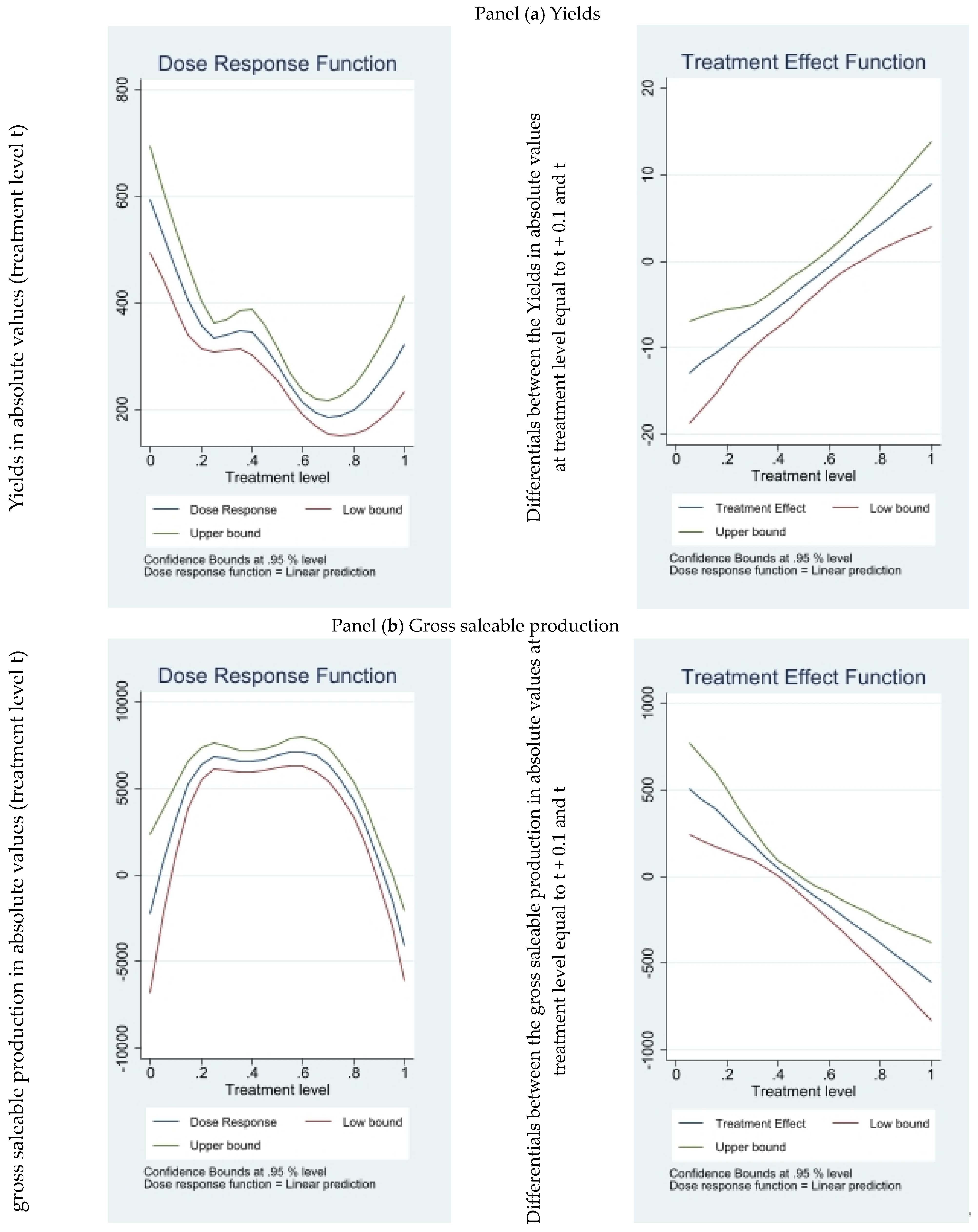
Overall, IWR exerts a significant effect on yields as depicted by the DRF (Figure 5a) (RQ1). The left-side panel of the figures reports the DRF providing graphical representations of the relationship between WD and yields, while the right-side panel depicts the TEF, that is, the first derivative of the respective DRF. The middle line refers to the function, while the top and bottom lines represent 95% confidence intervals. See Table A3 for model validation. This result is mainly in line with Tack et al. [16] that demonstrated how irrigation is an effective tool to support yield, even if with extreme climate change conditions, and Zaveri and Lobell [17] that concluded a positive increasing benefit of irrigation on wheat yields.
Some differences, however, emerge when we look at different treatment levels (RQ2). The dose–response function has, in fact, a convex form (with the exception of treatment levels between 0.2 and 0.4) suggesting that the positive effect of irrigation on yields emerges only for a high level of treatment (irrigation). The TEF, which reports the outcome as increasing due to the unitary increment of the treatment, confirms it: the effect increased more for the last third of the treatment distribution.
The convex form of the DRF reversed and became concave when considering the impact of irrigation on gross saleable production (Figure 5, Panel b). The former indeed positively affects the latter, but following a decreasing path, as highlighted by the TEF: once the maximum has been reached, to increase the treatment leads to a loss in gross saleable production.
Overall, these results confirm the existing literature. Ruberto et al. [15] found that irrigation is a determinant factor affecting crops’ economic values, but it is not more relevant than other internal and external elements.
3.2. Heterogeneity Analysis
The effect of irrigation can be influenced by the agronomic characteristics of different crops and their higher or lower water intensity nature. This heterogeneity has been underlined by Li and Troy [18] concluding that some crops are unsustainable given that they need too much water.
Crop differences also emerged in this paper. By looking at the DRFs of Figure 5a: some crops are characterized by high yield volumes yields and low IWR volumes (before treatment level 0.4) while others by low yield volumes and high IWR volumes (between 0.4 and 1). Therefore, we decided to investigate this heterogeneity, especially whether the effect of the treatment differs across crops (RQ3). Therefore, we replicated the analysis by splitting the sample into two-subsamples according to the yield, above and below 350 quintal/ha. The first sample included lower water intensity crops, whereas the second one included higher water intensity crops. Descriptives for the subsamples are provided by Table 2 and Table 3 and suggest that while crops included in the group above the turning point are mainly non-arboreal crops, the other group is mainly composed by arboreal crops which account for higher irrigation water requirements, but also for higher gross saleable production.
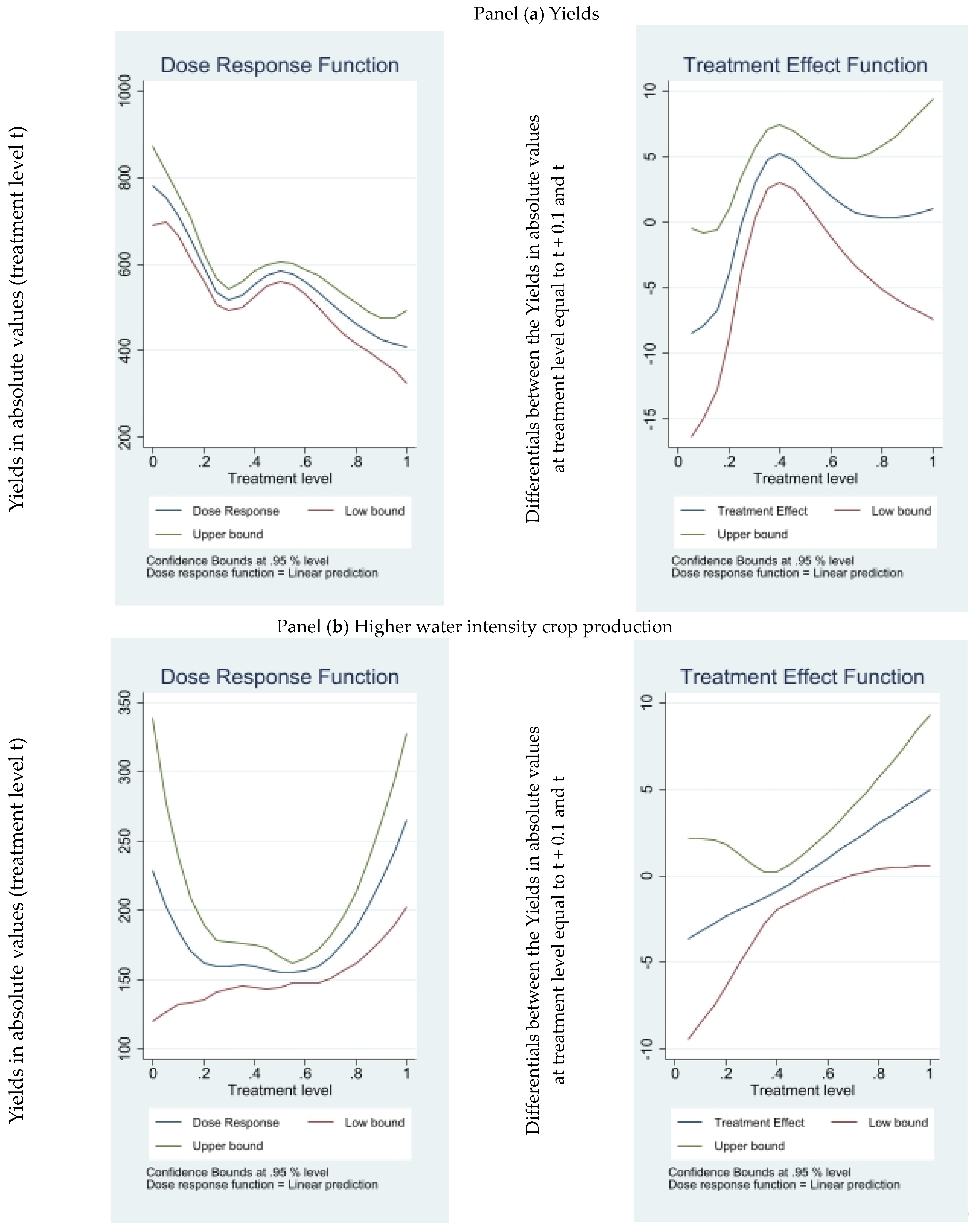
Starting from the effects on yields and lower water intensity crop production (Figure 6a), the left-side panel of the figures reports the DRF providing graphical representations of the relationship between IWR and gross saleable production (a) and yields (b); the right-side panel depicts the TEF, that is, the first derivative of the respective DRF. The findings show that the DRF is concave for both the lowest and highest levels of the treatment, while it assumes a convex shape from 0.2 to 0.4. This evidence suggests that on average, there is a positive effect for a medium level of water irrigation, meaning that the yields of lower water intensity crops do not benefit from a low level of irrigation (as the treatment is not enough to increase yields) or from the highest ones (due to the decreasing marginal productivity of the production factors). Conversely, a medium level of treatment seems to be effective and generates positive and increasing effects.
In the case of higher water intensity crops (Figure 6b), a clearer convex pattern emerges. This suggests that water irrigation is effective in increasing yields only after a certain level of treatment (around 0.5), but after that, it will always remain positive.
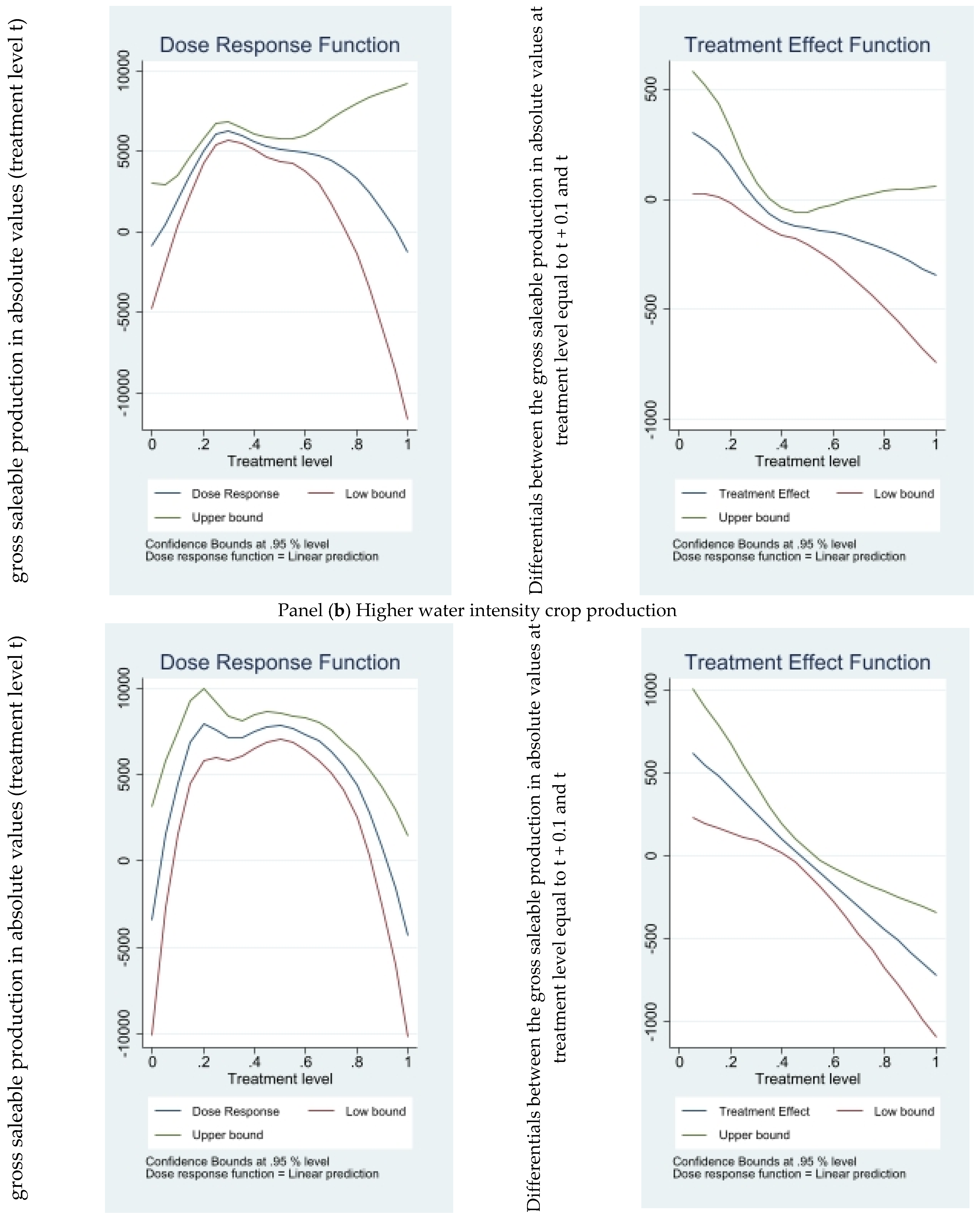
Moving to the gross saleable production estimations (Figure 7), lower water intensity crops (Figure 7a) show a concave DRF along the 0.1–0.6 treatment span (the only significant part of the estimations). In this case, in fact, the left-side panel of the figures also reports the DRF providing graphical representations of the relationship between IWR and gross saleable production (a) and yields (b); the right-side panel depicts the TEF, that is, the first derivative of the respective DRF. The results suggest that, on average, while there is a positive effect from the lower level of treatment, there is a negative effect from the highest levels. For higher water intensity crops (Figure 7b), the impact follows a similar trend: no significance before 0.1 and after 0.9, a positive impact corresponding to a lower level of treatment, a null impact for a medium level of treatment, and a negative one for the higher levels. This suggests that the economic value (i) noticeably benefits from obtaining the first level of treatment (moving from around zero irrigation to a certain degree of it) with a sharp increase in the gross saleable production and (ii) from a medium level of treatment, as they guarantee a certain and constant level of gross saleable production. From the economic perspective, treatment impact on gross saleable production follows the same logic as that of decreasing marginal productivity, as depicted by the TEF: the gains in gross saleable production decrease along the treatment increase, up to the point where they eventually became negative. The clear relevance of the treatment (irrigation) is what we observe in agronomic practices commonly implemented for arboreal crops, such as supplemental irrigation for vineyards.
If we split the group of higher water intensity crops according to the median value of the gross saleable production (Table 4), we find that the upper part is mostly made up of arboreal crops (A), which from the agronomic perspective requires more water irrigation, accounts for higher gross saleable production and maintains a constant economic value over time in comparison with non-arboreal crops (H).
4. Discussion and Conclusions
Following the heated debate on water crises and irrigation requirements in a climate change scenario, this study emphasizes the growing importance of irrigation water requirements in shaping governmental strategies for water allocation and management. The research estimates the economic impact of irrigation water requirements on yields and gross saleable production for 13 different crops in Italy over the 2010–2020 period by using GPS methods. The findings indicate:
- (i)
- a causal effect of irrigation water on economic value, with positive impacts observed for high levels of water irrigation in terms of crop yields (RQ1)
- (ii)
- in terms of yields, it is positive only for a high level of water irrigation, while gross saleable production reacts sharply and positively to a low level of treatment and negatively for a higher level of treatment; in the middle, it remains overall stable, but reaches different values depending on the sample (RQ2)
- (iii)
- the effect is mediated by the specific water requirements of different crops (RQ3).
We want to stress that we basically observed three types of crops: the first one (e.g., sugar beet) is characterized by high yield volumes, low water requirements but also low gross saleable production (the decreasing part up to the turning point of the GPS1); the second one is denoted by a lower yield volumes, but higher water requirements as well as higher gross saleable production (e.g., corn); the last one displays mostly arboreal crops which are extremely water demanding (e.g., Actinidia) and that, even though they are not too different in terms of yield volumes form the second group, they show the highest gross saleable production.
Therefore, in terms of water allocation strategies, our findings highlight the need for tailored strategies. The results suggest that, when farmers face strong constraints on water availability, the more efficient solution seems to be to allocate water to arboreal crops, as the effect of water irrigation on gross saleable production is positive also if small quantities of water are distributed. However, to maintain the highest economic values, a medium level of water allocation is needed. This is in line with the core of efficiency criterion in economics: as depicted in [36], it is better to allocate water to the production of crops for which the productivity is higher. In our case, this has been demonstrated in the case of arboreal crops, confirming what the literature has said while focusing on Norther Italian regions [37].
Crops that need lower levels of water appear as the crops that farmers and policy makers should look at not only due to their relevance to the final market (consumers), but also due to their use as inputs in other agrifood production processes. This is the case for alfalfa used in Parmigiano Reggiano PDO production, one of the main economically successful agrifood products of Italy [37]. To what extent crops participate in food value chains, both at the national and global level, should therefore be considered when designing strategic water management strategies. It can have an effect not only on the sustainability of local production systems, but also on their economic competitiveness.
From a policy perspective, this paper highlights how water resource management and governance questions should be addressed by considering both yields and economic value, rather than focusing only on the productivity [38]. Our contribution stresses that it would be a mistake and economically damaging to consider only low water demanding crops as feasible under water scarcity scenarios. This evidence, at least in part, supports the mitigation strategies that have been supported by policy interventions and plans over the last several years.
In addition, given that arboreal crops are crops in which unconventional water use is allowed (i.e., direct and indirect use of wastewater), the importance of arboreal crops in crop allocation becomes even more apparent [39]. Arboreal crops are, in fact, the only type for which the use of wastewater is allowed. The reuse of wastewater is supported by the EU in order to achieve a more sustainable agricultural system. However, its efficiency depends on how policies and interventions are designed.
For example, in the EU, Regulation 2020/741/EU addresses water scarcity issues by introducing a harmonized standard for wastewater reuse in agriculture. The achievement of the best possible solution can be challenging, especially in countries which lack a consistent normative system in regard to the second half of the water utilization cycle, i.e., the depuration and discharge of wastewater. Indeed, the lack of good territorial and crop-tailored regulations is a major driver of the increase in soil and crop damage. With the aim of maximizing the availability of water for farmers, policy makers and local actors have to consider not only natural boundaries and water quality [40], but also economic factors, such as infrastructure costs and the determination of water prices [41]. The provision of high-quality water provided by so-called direct reuse may result in higher prices, which can be unsustainable for farmers, especially those that cultivate low value-added crops. From the economic perspective, the concept of “irrigation water consumption-yield-economic value of crops” should be balanced by adopting a more inclusive and sustainable approach. Even if the main issue remains the problem of maximum optimization between productivity, economic values and physical constraints (water in this case), nowadays, the issue should also be enriched by a more comprehensive sustainability strategy. This is particularly clear if we look, for example, at the Sustainable Development Goals Agenda (SDGs) which attempts to simultaneously achieve the protection, restoration and promotion of the sustainable use of terrestrial ecosystems (SDG 15) and the sustainable management and provision of clean water (SDG 6) with an increase in agriculture productivity (SDG 2). The result, therefore, is a complex challenge of supporting agricultural productivity, with efficient high quality water use, while providing long-term environmental, social and economic sustainability to farmers and citizens. Therefore, to address this issue it is not sufficient to look at yields, but we also need to consider the economic dimension of crops from a more integrated point of view.
Our findings should be considered as explorative and further research needs to be carried out. The estimation of the socio-economic effects of specific irrigation techniques and, in particular, the adoption of wastewater reuse in agriculture is in our research agenda. At the same time, we are interested in investigating how technological choices and socio-cultural dynamics will produce patterns of water use and allocation.
Author Contributions
P.S.: investigation, data curation, methodology, writing—original draft. C.V.-P.: data curation, methodology, validation, writing—review and editing. F.C.: data curation, writing—review and editing. R.Z.: supervision. All authors have read and agreed to the published version of the manuscript.
Funding
This work was in part funded by the Next Generation EU – Italian National Recovery and Resilience Plan (NRRP), Mission 4, Component C2, Investment 1.1, “Fondo per il Programma Nazionale di Ricerca e Progetti di Rilevante Interesse Nazionale (PRIN)” (Directorial Decree n. 2022/1409)—under the project "MUlti-scale modelization toward Socio-ecological Transition for Water management (MUST4Water)", n. P2022R8ZTW. This work reflects only the authors’ views and opinions, neither the Ministry for University and Research nor the European Commission.
Data Availability Statement
Data available on request due to restrictions.
Conflicts of Interest
The authors declare no conflicts of interest.
Appendix A

Table A1.
Crops and NUTS3.
| Crops | Actinidia, Alfalfa, Corn, Grape, Green bean, Melon, Onion, Peach, Pear, Potato, Soy, Sugar beet, Tomato (Processing) | ||||||||
|---|---|---|---|---|---|---|---|---|---|
| NUTS3-Provinces | ITH51-Piacenza (PC), ITH52-Parma (PR), ITH53-Reggio Emilia (RE), ITH54-Modena (MO), ITH55-Bologna (BO), ITH56-Ferrara (FE), ITH57-Ravenna (RA), ITH58-Forlì-Cesena (FC) | ||||||||
| BO | FC | FE | MO | PC | PR | RA | RE | Total | |
| Actinidia | 10 | 11 | 6 | 0 | 0 | 0 | 11 | 0 | 38 |
| Alfalfa | 3 | 2 | 0 | 6 | 8 | 7 | 1 | 9 | 36 |
| Corn | 11 | 0 | 11 | 11 | 9 | 9 | 11 | 10 | 72 |
| Grape | 11 | 11 | 0 | 11 | 2 | 5 | 11 | 8 | 59 |
| Green bean | 0 | 8 | 0 | 0 | 6 | 0 | 10 | 0 | 24 |
| Melon | 8 | 0 | 11 | 5 | 0 | 0 | 0 | 0 | 24 |
| Onion | 11 | 8 | 0 | 0 | 9 | 0 | 10 | 0 | 38 |
| Peach | 11 | 11 | 11 | 9 | 0 | 0 | 11 | 0 | 53 |
| Pear | 11 | 0 | 11 | 10 | 0 | 0 | 11 | 7 | 50 |
| Potato | 11 | 9 | 7 | 0 | 0 | 0 | 11 | 0 | 38 |
| Soy | 7 | 0 | 8 | 8 | 8 | 0 | 7 | 7 | 45 |
| Sugar beet | 11 | 7 | 11 | 9 | 6 | 8 | 11 | 9 | 72 |
| Tomato (Processing) | 8 | 5 | 10 | 0 | 11 | 9 | 11 | 6 | 60 |
| Total | 113 | 72 | 86 | 69 | 59 | 38 | 116 | 56 | 609 |
Table A2.
Data definitions.
| Source | Variable | Definition |
|---|---|---|
| Fadn | Economic Dimension of Farms | Average economic dimension of farms, by year and at NUTS3 level. Values from 1 (small) to 5 (big) |
| Gross Saleable Production | Gross saleable production for irrigated crops (EUR), by year and crop, at NUTS3 level | |
| Arpae | IS_TNover90p | Number of days during IS in which the minimum temperature went above the 90th percentile of its 1961–2020 distribution. |
| IS_TXover90p | Number of days during IS in which the maximum temperature went above the 90th percentile of its 1961–2020 distribution. | |
| TN_HWN | Number of minimum temperature heatwaves during the IS. | |
| TX_HWN | Number of minimum temperature heatwaves during the IS. | |
| IS_rainydays | Number of days with effective rainfall during the IS. | |
| IS_Heavyrainydays | Number of days with heavy rainfall during the IS. | |
| Cer | Yields | Yields of irrigated crops (quintals/ha), by year and crop, at NUTS3 level. |
| Acreage | Acreage of irrigated crops (ha), by year and crop, at NUTS3 level. | |
| Irriframe | IWR | Average irrigation water requirement over the exact period of its irrigation (mm/ha), by year and crop, at NUTS3 level. |
| Eurostat | Percapita_GDP | Per capita Gross Domestic Product at current market prices (EUR), by year, at NUTS3 level. |
Table A3.
Estimation of the DRF.
| GPS 1-Full Sample | ||||
|---|---|---|---|---|
| IYields (Quintals/Ha) | Gross Saleable Production (EUR /Ha) | |||
| Variable | Coefficients | SE | Coefficients | SE |
| WD | −865.569 | 599.9565 | 57,081.63 *** | 14,732.31 |
| WD (^2) | 656.8621 | 525.6152 | −58,377.29 *** | 13,250.4 |
| GPS | −175.9433 | 190.391 | −3111.61 | 4472.597 |
| GPS^2 | 285.0726 | 153.6744 | −69.52433 | 3595.859 |
| WD *GPS | −154.2393 | 233.6022 | −5216.351 | 5469.356 |
| Observations | 609 | 588 | ||
| GPS2 Lower (a) and Higher (b) Water Intensity Crops | ||||
| A-IYields (Quintals/Ha) | B-IYields (Quintals/Ha) | |||
| Variable | Coefficients | SE | Coefficients | SE |
| WD | −894.4823 * | 513.8982 | −412.9934 | 341.7621 |
| WD (^2) | 471.4249 | 472.1137 | 454.8758 | 288.6213 |
| GPS | −356.091 ** | 167.6097 | 52.81079 | 101.4106 |
| GPS^2 | −29.08193 | 133.5734 | −2.967697 | 78.13132 |
| WD *GPS | 1059.992 *** | 224.9905 | −46.00546 | 116.1592 |
| Observations | 214 | 395 | ||
| GPS3- Lower (a) and Higher (b) Water Intensity Crops | ||||
| A-Gross Saleable Production (EUR/Ha) | B-Gross Saleable Production (EUR/Ha) | |||
| Variable | Coefficients | SE | Coefficients | SE |
| WD | 34,052.73 ** | 14,480.93 | 69,529.67 *** | 22,686.64 |
| WD (^2) | −33,620.69 ** | 13,692.91 | −70,070.87 *** | 19,574.33 |
| GPS | 6062.368 | 4580.525 | −13,683.88 ** | 6411.992 |
| GPS^2 | −697.1769 | 3628.13 | 7233.836 | 4917.609 |
| WD *GPS | −17,208.59 *** | 6118.141 | −2564.918 | 7392.32 |
| Observations | 210 | 378 | ||
Notes: *** p < 0.01, ** p < 0.05, * p < 0.1.
References
- Di Paola, A.; Di Giuseppe, E.; Pasqui, M. Climate Stressors’ Interplays Modulating Interannual Olive and Grapevine Yields in Italy: A Composite Index Approach. In Proceedings of the 17th Plinius Conference on Mediterranean Risks, Frascati, Italy, 18–21 October 2022. [Google Scholar]
- European Commission. Joint Research Centre. JRC MARS Bulletin: Crop Monitoring in Europe. Vol. 30 No 3, 21 March 2022.; Publications Office: Luxembourg, 2022. [Google Scholar]
- European Commission. Joint Research Centre. JRC MARS Bulletin: Crop Monitoring in Europe. Vol. 31 No 3, March 2023.; Publications Office: Luxembourg, 2023. [Google Scholar]
- Pronti, A.; Auci, S.; Di Paola, A.; Mazzanti, M. What Are the Factors Driving the Adoption of Sustainable Irrigation Technologies in Italy? In Proceedings of the “Tomorrow’s Food: Diet transition and its implications on health and the environment”, Pistoia, Italy, 13 June 2019. [Google Scholar]
- Water Scarcity Conditions in Europe (Water Exploitation Index plus)-8th EAP; European Environment Agency: Copenhagen, Denmark, 2019.
- Eurostat. Agri-Environmental Indicator-Irrigation. 2016. Available online: https://ec.europa.eu/eurostat/statistics-explained/index.php?title=Agri-environmental_indicator_-_irrigation#:~:text=In%202016%2C%208.9%20%25%20of%20utilised,and%20irrigated%20areas%20by%206.1%20%25. (accessed on 19 October 2023).
- European Commission. Joint Research Centre. JRC MARS Bulletin: Crop Monitoring in Europe. Vol. 30, No 7, July 2022.; Publications Office: Luxembourg, 2022. [Google Scholar]
- European Commission. Joint Research Centre. JRC MARS Bulletin: Crop Monitoring in Europe. Vol. 31 No 7, July 2023.; Publications Office: Luxembourg, 2023. [Google Scholar]
- Van Der Velde, M.; Wriedt, G.; Bouraoui, F. Estimating Irrigation Use and Effects on Maize Yield during the 2003 Heatwave in France. Agric. Ecosyst. Environ. 2010, 135, 90–97. [Google Scholar] [CrossRef]
- Martínez-Lüscher, J.; Chen, C.C.L.; Brillante, L.; Kurtural, S.K. Mitigating Heat Wave and Exposure Damage to “Cabernet Sauvignon” Wine Grape With Partial Shading Under Two Irrigation Amounts. Front. Plant Sci. 2020, 11, 579192. [Google Scholar] [CrossRef] [PubMed]
- Schlenker, W.; Hanemann, W.M.; Fisher, A.C. Water Availability, Degree Days, and the Potential Impact of Climate Change on Irrigated Agriculture in California. Clim. Chang. 2007, 81, 19–38. [Google Scholar] [CrossRef]
- Villa-Cox, G.; Cavazza, F.; Jordan, C.; Arias-Hidalgo, M.; Herrera, P.; Espinel, R.; Viaggi, D.; Speelman, S. Understanding Constraints on Private Irrigation Adoption Decisions under Uncertainty in Data Constrained Settings: A Novel Empirical Approach Tested on Ecuadorian Cocoa Cultivations. Agric. Econ. 2021, 52, 985–999. [Google Scholar] [CrossRef]
- Zucaro, R. Atlante Nazionale Dell’irrigazione; INEA: Roma, Italy, 2011; ISBN 978-88-8145-228-6. [Google Scholar]
- Manganiello, V.; Banterle, A.; Canali, G.; Gios, G.; Branca, G.; Galeotti, S.; De Filippis, F.; Zucaro, R. Economic Characterization of Irrigated and Livestock Farms in The Po River Basin District. Econ. Agro-Aliment. 2022, 23, 1–24. [Google Scholar] [CrossRef]
- Ruberto, M.; Catini, A.; Lai, M.; Manganiello, V. The Impact of Irrigation on Agricultural Productivity: The Case of FADN Farms in Veneto. Econ. Agro-Aliment. 2022, 23, 1–20. [Google Scholar] [CrossRef]
- Hirano, K.; Imbens, G.W. The Propensity Score with Continuous Treatments. In Wiley Series in Probability and Statistics; Gelman, A., Meng, X., Eds.; Wiley: Hoboken, NJ, USA, 2004; pp. 73–84. ISBN 978-0-470-09043-5. [Google Scholar]
- Negri, D.H.; Gollehon, N.R.; Aillery, M.P. The Effects of Climatic Variability on US Irrigation Adoption. Clim. Change 2005, 69, 299–323. [Google Scholar] [CrossRef]
- Cunha, D.A.D.; Coelho, A.B.; Féres, J.G.; Braga, M.J. Effects of Climate Change on Irrigation Adoption in Brazil. Acta Sci. Agron. 2014, 36, 1–9. [Google Scholar] [CrossRef]
- Seo, S.N. An Analysis of Public Adaptation to Climate Change Using Agricultural Water Schemes in South America. Ecol. Econ. 2011, 70, 825–834. [Google Scholar] [CrossRef]
- Tack, J.; Barkley, A.; Hendricks, N. Irrigation Offsets Wheat Yield Reductions from Warming Temperatures. Environ. Res. Lett. 2017, 12, 114027. [Google Scholar] [CrossRef]
- Zaveri, E.; Lobell, D.B. The Role of Irrigation in Changing Wheat Yields and Heat Sensitivity in India. Nat. Commun. 2019, 10, 4144. [Google Scholar] [CrossRef] [PubMed]
- Li, X.; Troy, T.J. Changes in Rainfed and Irrigated Crop Yield Response to Climate in the Western US. Environ. Res. Lett. 2018, 13, 064031. [Google Scholar] [CrossRef]
- Determining the Economic Value of Water: Concepts and Methods, 2nd ed.; Young, R.A. (Ed.) RFF Press: New York, NY, USA, 2014; ISBN 978-0-415-83846-7. [Google Scholar]
- Mesa-Jurado, M.A.; Martin-Ortega, J.; Ruto, E.; Berbel, J. The Economic Value of Guaranteed Water Supply for Irrigation under Scarcity Conditions. Agric. Water Manag. 2012, 113, 10–18. [Google Scholar] [CrossRef]
- Faux, J.; Perry, G.M. Estimating Irrigation Water Value Using Hedonic Price Analysis: A Case Study in Malheur County, Oregon. Land Econ. 1999, 75, 440. [Google Scholar] [CrossRef]
- Antolini, G.; Auteri, L.; Pavan, V.; Tomei, F.; Tomozeiu, R.; Marletto, V. A Daily High-Resolution Gridded Climatic Data Set for Emilia-Romagna, Italy, during 1961-2010: EMILIA-ROMAGNA DAILY GRIDDED CLIMATIC DATA SET. Int. J. Climatol. 2016, 36, 1970–1986. [Google Scholar] [CrossRef]
- Perkins, S.E.; Alexander, L.V. On the Measurement of Heat Waves. J. Clim. 2013, 26, 4500–4517. [Google Scholar] [CrossRef]
- Giannerini, G.; Genovesi, R. The Water Saving with Irriframe Platform for Thousands of Italian Farms. J. Agric. Inform. 2015, 6. [Google Scholar] [CrossRef]
- Cavazza, F.; Galioto, F.; Raggi, M.; Viaggi, D. Ambiguity, Familiarity and Learning Behavior in the Adoption of ICT for Irrigation Management. Water 2022, 14, 3760. [Google Scholar] [CrossRef]
- Rosenbaum, P.R.; Rubin, D.B. The Central Role of the Propensity Score in Observational Studies for Causal Effects. Biometrika 1983, 70, 41–55. [Google Scholar] [CrossRef]
- Stuart, E.A. Matching Methods for Causal Inference: A Review and a Look Forward. Stat. Sci. 2010, 25. [Google Scholar] [CrossRef]
- De Simone, E.; Giua, M.; Vaquero-Piñeiro, C. Eat, Visit, Love. World Heritage List and Geographical Indications: Joint Acknowledgement and Consistency as Drivers of Tourism Attractiveness in Italy. Tour. Econ. 2023. [Google Scholar] [CrossRef]
- Crescenzi, R.; De Filippis, F.; Giua, M.; Salvatici, L.; Vaquero-Piñeiro, C. From Local to Global, and Return: Geographical Indications and FDI in Europe. Pap. Reg. Sci. 2023, 102, 985–1006. [Google Scholar] [CrossRef]
- Imbens, G.W. Nonparametric Estimation of Average Treatment Effects Under Exogeneity: A Review. Rev. Econ. Stat. 2004, 86, 4–29. [Google Scholar] [CrossRef]
- Bia, M.; Mattei, A. A Stata Package for the Estimation of the Dose-Response Function through Adjustment for the Generalized Propensity Score. Stata J. Promot. Commun. Stat. Stata 2008, 8, 354–373. [Google Scholar] [CrossRef]
- Tsur, Y. Economic Aspects of Irrigation Water Pricing. Can. Water Resour. J. 2005, 30, 31–46. [Google Scholar] [CrossRef]
- Zucaro, R. Condizionalità ex ante per le Risorse Idriche: Opportunità e Vincoli per il Mondo Agricolo; INEA, 2014; Available online: https://arts.units.it/retrieve/handle/11368/2836237/29019/Valore_irrigazione.pdf (accessed on 19 October 2023).
- Rising, J.; Devineni, N. Crop Switching Reduces Agricultural Losses from Climate Change in the United States by Half under RCP 8.5. Nat. Commun. 2020, 11, 4991. [Google Scholar] [CrossRef]
- Cervantes-Gaxiola, M.E.; Sosa-Niebla, E.F.; Hernández-Calderón, O.M.; Ponce-Ortega, J.M.; Ortiz-del-Castillo, J.R.; Rubio-Castro, E. Optimal Crop Allocation Including Market Trends and Water Availability. Eur. J. Oper. Res. 2020, 285, 728–739. [Google Scholar] [CrossRef]
- Jaramillo, M.; Restrepo, I. Wastewater Reuse in Agriculture: A Review about Its Limitations and Benefits. Sustainability 2017, 9, 1734. [Google Scholar] [CrossRef]
- Al-Hazmi, H.E.; Mohammadi, A.; Hejna, A.; Majtacz, J.; Esmaeili, A.; Habibzadeh, S.; Saeb, M.R.; Badawi, M.; Lima, E.C.; Mąkinia, J. Wastewater Reuse in Agriculture: Prospects and Challenges. Environ. Res. 2023, 236, 116711. [Google Scholar] [CrossRef]

Figure 2.
Days over the 90th percentile for minimum and maximum temperature (left) and number of heatwaves (right). Author’s elaboration on ARPA-E data. Notes: IS_TNover90p and IS_TXover90p expressed as number of days, while TN_HWN and TX_HWN as number of heatwaves.
Figure 2.
Days over the 90th percentile for minimum and maximum temperature (left) and number of heatwaves (right). Author’s elaboration on ARPA-E data. Notes: IS_TNover90p and IS_TXover90p expressed as number of days, while TN_HWN and TX_HWN as number of heatwaves.

Figure 3.
Temperature and precipitation at NUTS3 level. Author’s elaborations on ARPA-E data. Notes: IS_TNover90p, IS_TXover90p and IS_rainydays expressed as number of days.
Figure 3.
Temperature and precipitation at NUTS3 level. Author’s elaborations on ARPA-E data. Notes: IS_TNover90p, IS_TXover90p and IS_rainydays expressed as number of days.

Figure 4.
Wit and Yit by NUTS_3 area. Authors’ elaborations on CER and Arpae data. Notes: Wit is expressed in mm/ha/year and Yit is expressed in quintals/ha/year.
Figure 4.
Wit and Yit by NUTS_3 area. Authors’ elaborations on CER and Arpae data. Notes: Wit is expressed in mm/ha/year and Yit is expressed in quintals/ha/year.

Figure 5.
GPS1-Effects of irrigation on yields (Panel a) and gross saleable production (Panel b). Full sample. Panel (a) yields. Notes: We used bootstrap methods to obtain the dose–response function standard errors and confidence intervals which are included in the figures as the lower and upper bounds [35]. Models have been estimated with the constant. Yields are expressed in quintals/ha.

Figure 6.
GPS2-Effects of IWR on yields. Panel (a) Lower water intensity crop production. Notes: The middle line refers to the function, while the top and bottom lines represent 95% confidence intervals. We use bootstrap methods to obtain the dose–response function standard errors and confidence intervals which are included in the figures as lower and upper bounds [35]. Models have been estimated with the constant. Yields are expressed in quintals/ha and gross saleable production is considered at current prices.

Figure 7.
GPS3-Effects of irrigation water requirements on gross saleable production. Panel (a) Lower water intensity crop production. Notes: The middle line refers to the function, while the top and bottom lines represent 95% confidence intervals. We use bootstrap methods to obtain the dose–response function standard errors and confidence intervals which are included in the figures as lower and upper bounds [35]. Models have been estimated with the constant. Yields are expressed in quintals/ha and gross saleable production is considered at current prices.

Table 1.
Variables used in our analysis and their source. Author’s elaboration.
| Source | Variable | Obs | Mean | Std. Dev. | Min | Max |
|---|---|---|---|---|---|---|
| FADN | Economic Dimension of Farms | 609 | 3.289 | 0.329 | 2.327 | 4.389 |
| Gross Saleable Production (EUR) | 588 | 6427 | 4811 | 379.7 | 28,442 | |
| Arpae | IS_TNover90p (number of days) | 609 | 41.75 | 11.87 | 8 | 67 |
| IS_TXover90p (number of days) | 609 | 49.43 | 13.53 | 15 | 81 | |
| TN_HWN (number of heatwaves) | 609 | 5.156 | 1.457 | 1 | 8 | |
| TX_HWN (number of heatwaves) | 609 | 6.350 | 1.843 | 3 | 11 | |
| IS_rainydays (number of days) | 609 | 56.99 | 12.89 | 33 | 85 | |
| IS_Heavyrainydays (number of days) | 609 | 4.210 | 2.815 | 0 | 16 | |
| Cer-ISTAT | Yields (quintals/ha) | 609 | 301.6 | 214.6 | 22 | 850 |
| Acreage (ha) | 584 | 5919 | 10,055 | 32.96 | 133,905 | |
| Irriframe | IWR (mm/ha) | 609 | 33.95 | 12.48 | 8.048 | 74.47 |
| Eurostat | Percapita_GDP (million EUR) | 609 | 32,942 | 4476 | 23,972 | 42,403 |
Table 2.
Descriptive statistics.
| Lower Water Intensity Crops | |||
|---|---|---|---|
| Crop | Freq. | Percent | Cum. |
| Alfalfa | 13 | 6.070 | 6.070 |
| Melon | 1 | 0.470 | 6.540 |
| Onion | 36 | 16.82 | 23.36 |
| Potato | 32 | 14.95 | 38.32 |
| Sugar beet | 72 | 33.64 | 71.96 |
| Tomato (Processing) | 60 | 28.04 | 100 |
| Total | 214 | 100 | |
| Higher Water Intensity Crops | |||
| Actinidia | 38 | 9.620 | 9.620 |
| Alfalfa | 23 | 5.820 | 15.44 |
| Corn | 72 | 18.23 | 33.67 |
| Grapes | 59 | 14.94 | 48.61 |
| Green bean | 24 | 6.080 | 54.68 |
| Melon | 23 | 5.820 | 60.51 |
| Onion | 2 | 0.510 | 61.01 |
| Peach | 53 | 13.42 | 74.43 |
| Pear | 50 | 12.66 | 87.09 |
| Potato | 6 | 1.520 | 88.61 |
| Soy | 45 | 11.39 | 100 |
| Total | 395 | 100 | |
Table 3.
Gross saleable production and IWR.
| Lower Water Intensity Crops | |||||
|---|---|---|---|---|---|
| Variable | Obs | Mean | Std. Dev. | Min | Max |
| Gross Saleable Production | 210 | 5280 | 3214 | 624.5 | 20,537 |
| IWR | 214 | 29.25 | 11.09 | 8.048 | 72.95 |
| Higher Water Intensity Crops | |||||
| Gross Saleable Production | 378 | 7065 | 5401 | 379.7 | 28,442 |
| IWR | 395 | 36.49 | 12.47 | 8.933 | 74.47 |
Table 4.
Higher 50% gross saleable production.
| Variable | Obs | Mean | Std. Dev. | Min | Max |
|---|---|---|---|---|---|
| A_Gross Saleable Production | 159 | 11,552 | 4293 | 6471 | 28,442 |
| H_Gross Saleable Production | 31 | 10,251 | 4141 | 6518 | 26,846 |
| A_IWR | 164 | 36.35 | 10.02 | 9.918 | 57.77 |
| H_IWR | 43 | 33.69 | 16.39 | 8.933 | 74.47 |
| A_Yields | 164 | 202.3 | 62.43 | 58 | 320 |
| H_Yields | 43 | 228.4 | 94.39 | 51.19 | 320 |
Disclaimer/Publisher’s Note: The statements, opinions and data contained in all publications are solely those of the individual author(s) and contributor(s) and not of MDPI and/or the editor(s). MDPI and/or the editor(s) disclaim responsibility for any injury to people or property resulting from any ideas, methods, instructions or products referred to in the content. |
© 2023 by the authors. Licensee MDPI, Basel, Switzerland. This article is an open access article distributed under the terms and conditions of the Creative Commons Attribution (CC BY) license (https://creativecommons.org/licenses/by/4.0/).
Share and Cite
MDPI and ACS Style
Scatolini, P.; Vaquero-Piñeiro, C.; Cavazza, F.; Zucaro, R. Do Irrigation Water Requirements Affect Crops’ Economic Values? Water 2024, 16, 77. https://doi.org/10.3390/w16010077
AMA Style
Scatolini P, Vaquero-Piñeiro C, Cavazza F, Zucaro R. Do Irrigation Water Requirements Affect Crops’ Economic Values? Water. 2024; 16(1):77. https://doi.org/10.3390/w16010077
Chicago/Turabian StyleScatolini, Paolo, Cristina Vaquero-Piñeiro, Francesco Cavazza, and Raffaella Zucaro. 2024. "Do Irrigation Water Requirements Affect Crops’ Economic Values?" Water 16, no. 1: 77. https://doi.org/10.3390/w16010077
Note that from the first issue of 2016, this journal uses article numbers instead of page numbers. See further details here.